Wind turbine wake measurements with automatically adjusting scanning trajectories in a multi-Doppler lidar setup

In the context of the Perdigão 2017 experiment, the German Aerospace Center (DLR) deployed three long-range scanning Doppler lidars with the dedicated purpose of investigating the wake of a single wind turbine at the experimental site. A novel method was tested for the first time to investigate wake properties with ground-based lidars over a wide range of wind directions. For this method, the three lidars, which were space- and time-synchronized using the WindScanner software, were programmed to measure with crossing beams at individual points up to 10 rotor diameters downstream of the wind turbine. Every half hour, the measurement points were adapted to the current wind direction to obtain a high availability of wake measurements in changing wind conditions. The linearly independent radial velocities where the lidar beams intersect allow the calculation of the wind vector at those points. Two approaches to estimating the prevailing wind direction were tested throughout the campaign. In the first approach, velocity azimuth display (VAD) scans of one of the lidars were used to calculate a 5 min average of wind speed and wind direction every half hour, whereas later in the experiment 5 min averages of sonic anemometer measurements of a meteorological mast close to the wind turbine became available in real time and were used for the scanning adjustment. Results of wind speed deficit measurements are presented for two measurement days with varying northwesterly winds, and it is evaluated how well the lidar beam intersection points match the actual wake location. The new method allowed wake measurements to be obtained over the whole measurement period, whereas a static scanning setup would only have captured short periods of wake occurrences.

1 Introduction

In state-of-the-art wind-energy research, the investigation of the flow field downstream of a wind turbine – i.e., in its wake – is currently a topic of high relevance for the siting and operation of turbines, especially in a typical configuration of a wind farm with multiple collocated turbines. For this purpose it is important to understand how high static and dynamic loads of neighboring turbines will be. This question cannot be universally answered without taking the atmospheric conditions into consideration, which have an effect on the wind speed deficit in the wake, its width and its propagation path. In order to describe wake dynamics beyond the typical engineering models (Göçmen et al., 2016), high-resolution numerical models (e.g., large-eddy simulations) have proven to be an adequate tool and can realistically reproduce wind turbine wakes in well-defined conditions (Englberger and Dörnbrack, 2016; Wu and Porté-Agel, 2011, 2012). Nonetheless, models need validation by real-world experiments. Capturing all the previously mentioned properties of a highly dynamic yet small-scale and local atmospheric feature like a wind turbine wake is a highly challenging task for wind measurement technology. It requires instruments that can sample wind speeds in a volume of the atmosphere in a short time and in a flexible way. While different measurement systems have been used – such as radars (Hirth et al., 2012), sodars (Barthelmie et al., 2003) and small remotely piloted aircraft (Wildmann et al., 2014) – it is lidar technology of different categories (pulsed and continuous wave) that has proven to be the most versatile tool for performing wake measurements because of the high availability and reliability, good resolution and flexible possibilities to probe the atmosphere especially with scanning systems.

Coherent Doppler lidar instruments for wind speed measurement have been widely used in atmospheric sciences since the late 20th century (Frehlich et al., 1998; Reitebuch et al., 2001; Smalikho, 2003). Because of their good performance within the atmospheric boundary layer, their high availability and capability to measure continuously, they have become increasingly interesting for wind-energy research as well (Emeis et al., 2007; Frehlich and Kelley, 2008). Conically scanning lidars (operating in the so-called velocity azimuth display, or VAD, mode) are useful for measuring vertical profiles of wind speed and wind direction in the range between 50 m and the boundary-layer top. They can also be used to estimate dissipation rate and turbulent kinetic energy (Kumer et al., 2016). More advanced scanning scenarios can be performed with instruments that have full hemispherical scanning capabilities and thus allow arbitrary volumes of the atmosphere to be scanned. Such systems have been deployed in the past to measure wind turbine wakes by scanning through them either horizontally (in so-called plan-position indicator, or PPI, mode) or vertically (in so-called range–height indicator mode, short: RHI) (Käsler et al., 2010; Smalikho et al., 2013), thus showing their propagation path. A drawback of measurements with single lidars is that only radial wind velocities along the line of sight of the laser beam can be retrieved. To overcome this limitation, multiple lidars can be deployed with intersecting beams that allow a geometric reconstruction of the meteorological wind components (Calhoun et al., 2006; Choukulkar et al., 2017; Drechsel et al., 2009; Mann et al., 2009; Newman et al., 2016). Examples for multi-lidar measurements of wind turbine wakes are for example Iungo et al. (2013), who placed dual-Doppler measurement points in the wake to retrieve vertical and horizontal wind speed at these points. Van Dooren et al. (2016) combined PPI scans to retrieve the horizontal wind speeds at hub height in the wake and its horizontal propagation.

Placing measurement points into the wake with ground-based lidars is not trivial, because wind direction and thus turbine yaw angle and wake position change over time, and the time that a fixed measurement point in space is measuring the wake can thus be very limited. A good way to overcome this problem is to place the lidar on the nacelle as it was done by Bingöl et al. (2009), Trujillo et al. (2011) and Aitken and Lundquist (2014). The logistics for a nacelle-based installation are, however, significantly more complex, and a single lidar on the nacelle will not be able to retrieve three-dimensional wind vector measurements directly.

In this study, we propose a new measurement strategy for ground-based lidars that aims at solving the issue of limited measurement time of the wake due to the turbine yawing during the measurements. The measurement strategy employs three ground-based scanning lidars whose scanning trajectories are synchronized and adapted in accordance with the prevailing wind direction to continuously measure a wind turbine wake. Since the scanning trajectories are able to adapt to the prevailing wind direction, the availability of wake measurements is expected to increase significantly in comparison to the static scanning.

The paper is structured as follows. Section 2 introduces the measurement campaign and the instrumental setup, Sect. 3 describes the methods to deduce turbine wake characteristics. In Sect. 4 the results are presented and discussed, and Sect.  5 concludes our study with a list of lessons learned and next steps for future work.

2 Experiment description

2.1 The Perdigão 2017 experiment

The Perdigão 2017 experiment (Fernando et al., 2018) is part of a series of campaigns associated with the NEWA (New European Wind Atlas) project (Mann et al., 2017) and took place in central Portugal in late spring and early summer 2017. The main goal of the experiment is to understand the flow field over two mountain ridges, which are nearly parallel to each other, with a distance of 1.4 km between them and a height of more than 200 m over the surrounding valley (see Fig. 1). The intensive operation period (IOP) was set from 1 May to 15 June. An extended measurement period with a reduced amount of equipment lasted for a whole year, i.e., from December 2016 until December 2017. A detailed description of the instrumentation and the research goals of all involved institutions is given in Fernando et al. (2018). On the southwest ridge of the Perdigão mountains, an Enercon E-82 wind turbine is installed. It is designed for low wind speeds and has a cut-in speed of 2 m s⁻¹. Nominal wind speed is 12 m s⁻¹ with a rated power of 2 MW. The hub height is 78 m a.g.l. (above ground level); the rotor diameter is 82 m. Data from the turbine are not yet available. At the same location, an initial, smaller campaign was carried out in 2015 and is described in Vasiljević et al. (2017) with all the logistical challenges attributed to the site. An analysis of wind turbine wake measurements of the 2015 experiment is presented in Menke et al. (2018). Many of the lessons that were learned in that first campaign were considered in the design of the presented campaign.

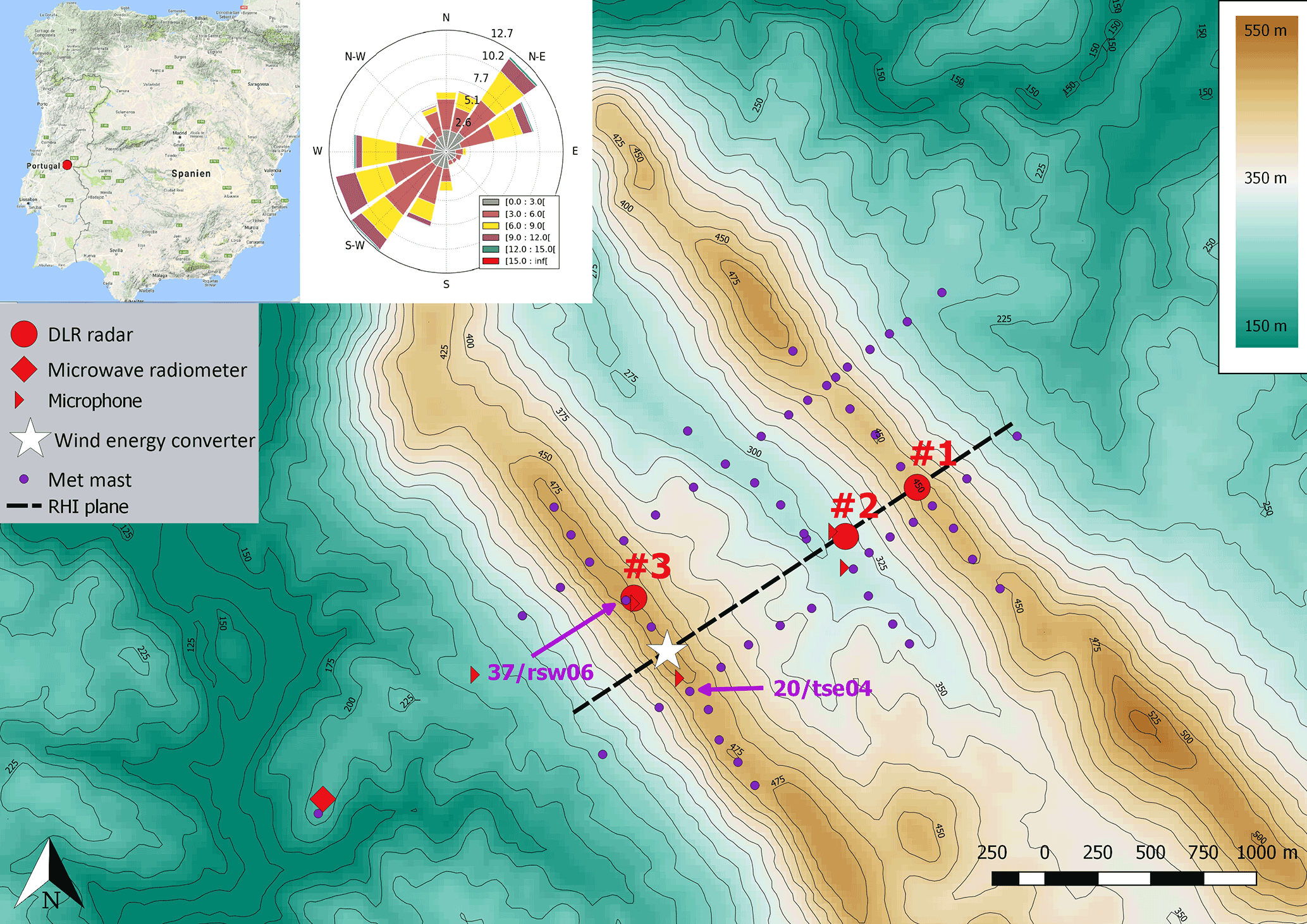
Figure 1 Map of the Perdigão site, including DLR instrumentation and meteorological mast locations. It also shows a wind rose for the sonic anemometer at 80 m on tower 20/tse04 for the IOP period. The dashed black line indicates the typical RHI scanning plane.

2.2 DLR instrumentation and lidar scanning strategy

The German Aerospace Center (DLR) contributed to the experiment with three long-range Doppler lidar systems of the type Leosphere Windcube 200S, upgraded to work in the WindScanner mode (Vasiljevic et al., 2016), a microwave radiometer of the type HATPRO-5G and several microphones. The research goals with these instruments are to study not only weather-dependent sound propagation of wind turbine noise but also the investigation of wakes in different atmospheric stability regimes. In this study, wake measurements of the lidar instruments are presented. A summary of the key features of the lidar systems is given in Table 1.

Table 1 Leosphere Windcube 200S specification overview. PRF stands for pulse repetition frequency; FFT stands for fast Fourier transform.

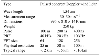
Figure 1 shows the location of the three lidars, denoted #1–3. The purpose for these locations is to have two instruments in line with the wind turbine in the main wind direction, which is from the southwest, one in the valley between the ridges and one on the distant mountain ridge, in order to be able to perform coplanar RHI scans. The third lidar could be used to cut the wake with RHI scans at several distances behind the turbine. The majority of the time during the campaign, the lidars were run in these standard kinds of scanning scenarios. The advantage compared to the experimental strategy described in the following is that these are well-established methods with little risk of problems with software or hardware of the lidars. Another advantage is that these RHI scans were of great benefit for other research goals of the experiment, namely the investigation of the flow in the valley and above. For wake characterization, unique two-dimensional flow visualizations of the wake could be captured for the main wind direction as presented in Wildmann et al. (2018). For those coplanar measurements it was important to have one lidar (#2) in the valley measuring radial wind speeds at a higher elevation angle compared to the lidar on the northeast ridge (#1). The siting of the lidars is always subject to logistical constraints, especially in a complex terrain as in Perdigão (Vasiljević et al., 2017). In the best case, lidar #2 would have been placed closer to the wind turbine and at a lower elevation, but the topography and availability of electrical power did not allow it. The analysis of coplanar and wake cut scans is not part of this study. Good wake measurements with the standard scanning scenarios are only possible in this setup if the wind is in a narrow angular range perpendicular to the ridges. For example, at an offset to the plane of 10^∘, the wake center will be 40 m from the scanning plane at a distance of 3 rotor diameters downstream of the turbine and thus not detectable by the coplanar scans any more. The locations of the lidar systems, however, also allow the wake to be measured in a wide area of northwesterly wind directions if the scanning trajectories are adapted accordingly. In this study, concepts are shown regarding how the availability of wake measurements can be increased by automatic adaptation of scanning scenarios with respect to the prevailing wind direction. The goal is to determine the wind conditions up to 10 rotor diameters downstream of the wind turbine at hub height. To achieve this, measurement points are defined in space where the three lidar beams will cross in order to reconstruct the wind vector. These points are placed equidistantly behind the wind turbine with a separation of 1 rotor diameter (i.e., 80 m). Additionally, on the later experiment days, one point was added 1 rotor diameter upstream, to measure the inflow of the turbine. In order to capture more of the wake with a single line-of-sight lidar measurement than just a single point, multiple range gates are added before and after the multi-Doppler measurement point. Figure 2 depicts this scanning scenario.

2.3 Planning and control of complex trajectories

The Danish Technical University (DTU) developed a special software called WindScanner Client Software (WCS) for the Windcube scanning lidar systems to synchronize multiple instruments in time and space, allowing scenarios with multiple crossing points in space. This feature is not available with standard lidar systems. With WindScanner a synchronization to millisecond accuracy by GPS timing and a few meters of spatial offset between the lidar beams by thorough calibration of the pointing direction and lidar position are feasible. The technical details of the software and hardware modifications to the Windcube lidar instrument are described in Vasiljevic (2014) and Vasiljevic et al. (2016).

While the WCS enables the low-level control of the lidars to synchronize predefined scenarios in multiple systems, it is up to the user to define these scenarios with matching azimuth, elevation and range gate distance for crossing lidar beams at predefined points. For this purpose, the authors have developed a planning tool based on Java and the NASA WorldWind virtual globe software development kit (NASA, 2018). It allows coordinates of measurement points in the geographical coordinate system to be specified (latitude, longitude, altitude) through either a text file list or mouse clicks on the virtual globe. The points and lidar beams are visualized on the 3-D virtual globe, and a simulation of the scans can be demonstrated. The parameters for all specified lidars will be automatically generated. Lidar-specific information about the measurement points – like pulse type to use, accumulation time and time to move between each measurement point – is defined in a settings tab for the whole scenario. Scenario files can be created and sent to the systems.

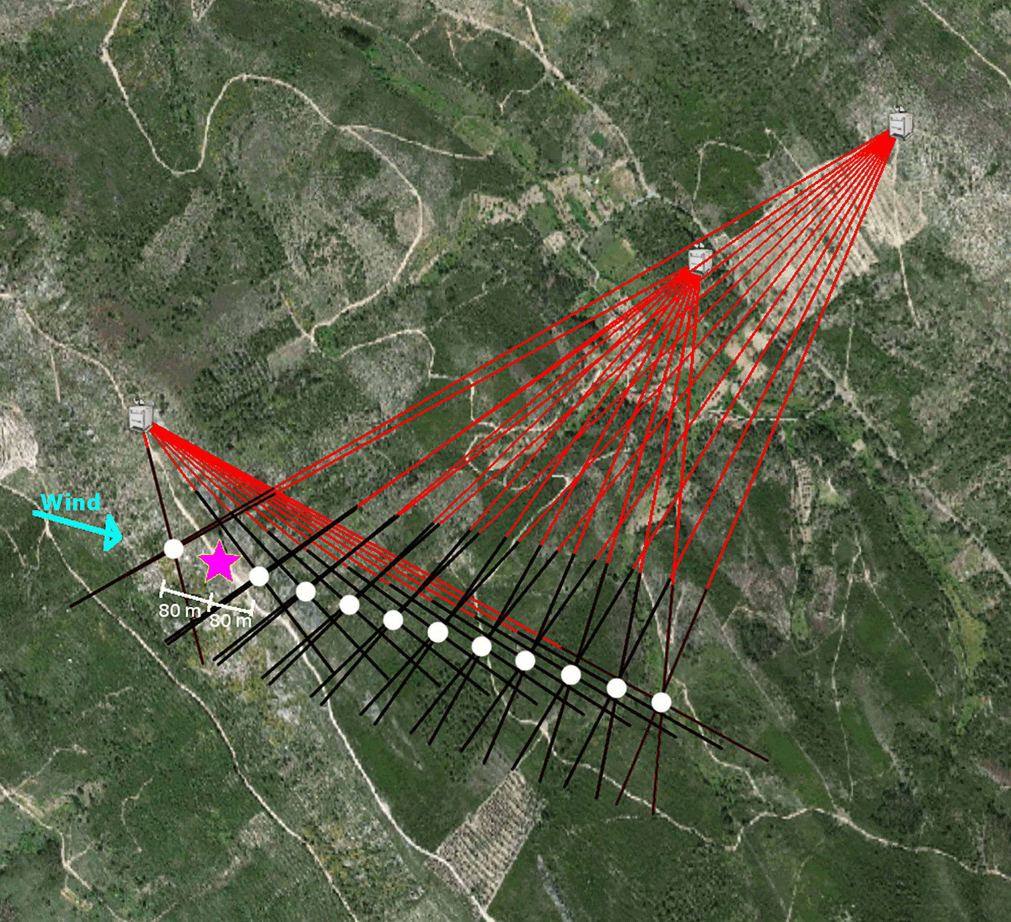
Figure 2 Visualization of multi-Doppler wake measurement scenario. Red represents the lidar beams, black represents the area with 2 m separated range gates, the pink star is the wind turbine and the white dots are the center range gates where lidar beams cross.

Selected commands as specified in the open protocol RSComPro (Vasiljevic et al., 2013) of the WindScanner software have been implemented to increase the level of interaction of the software with the lidar systems. The most important commands are “sending new scenarios” to a system and “starting” and “stopping” the measurements. The Java program will also receive current measurement data and display them upon request. Since synchronization of multiple systems is achieved by sending delays to the fastest system from the master computer, as described in Vasiljevic (2014), this task is also taken over by the Java program. Figure 3 shows a screenshot of the software in operation.

Figure 3 Example view of lidar planner software. On the left, the virtual globe with display of lidars and scanning scenario. On the right, the graphical user interface (GUI) for live data view. Other tabs in the program allow changing settings of the scenario, configuring the automatic scenario adaption etc.

2.4 Adaptation of scanning scenarios to wind direction

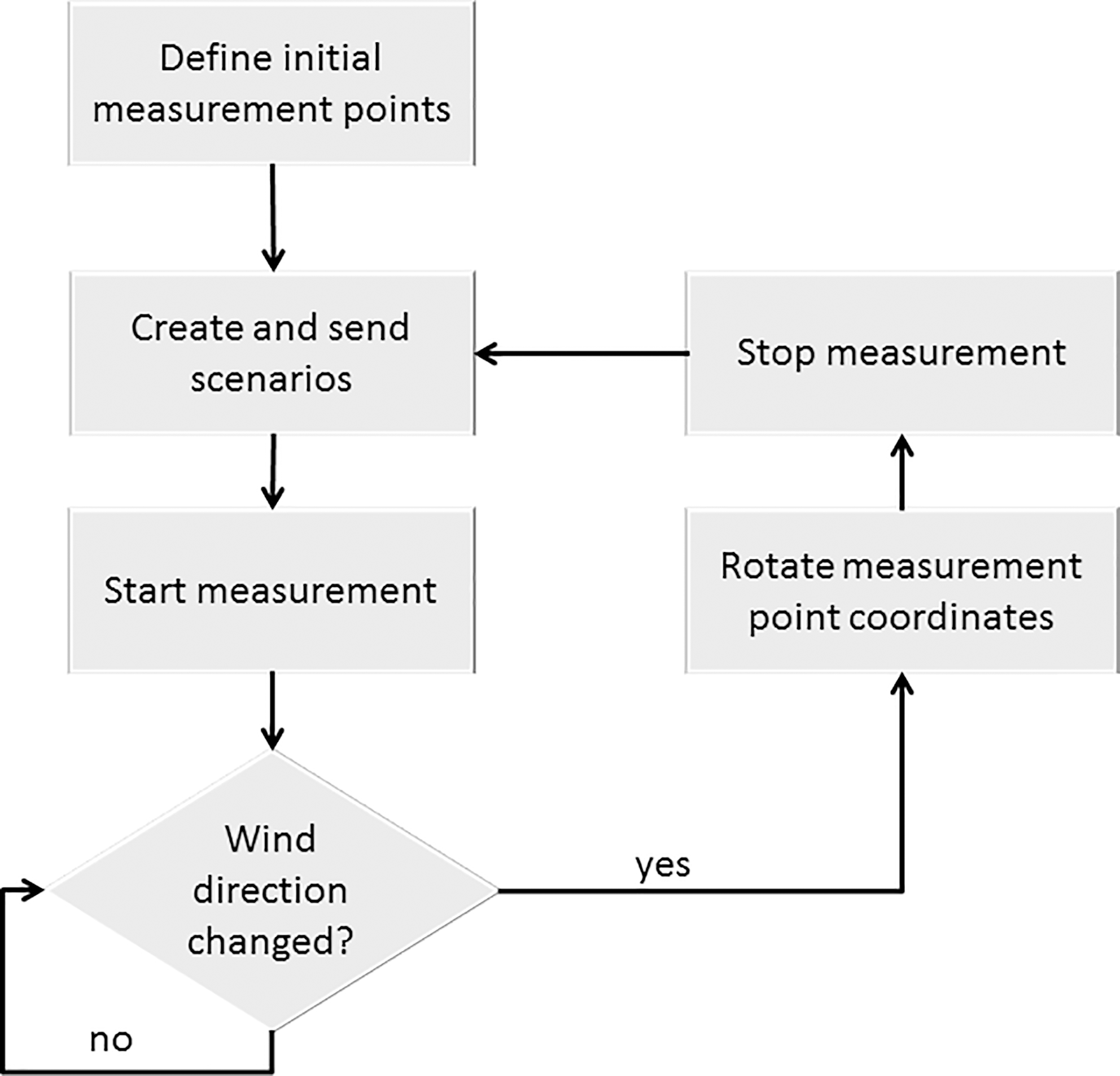
With the previously described software it has also been realized that a scenario can be adapted according to an external input. For the given experiment, the goal was to measure in the wake of the wind turbine, and thus the measurement points should be adjusted to be downstream of the wind turbine in the varying main wind direction. To achieve this, a rotation of the measurement points in the local coordinate system around the wind turbine position has been programmed, which is triggered by a new input of wind direction. The points are then rotated by the angular difference between the previous and the new wind direction. After new measurement point locations have been computed, the lidars are stopped, the new scenarios are sent to the systems and measurements are restarted (see Fig. 4). The time to restart the lidars with a new scenario can be as fast as 15 s, but it occasionally also takes longer (< 1 min) if the initialization of one of the system fails and needs to be repeated.

Figure 4 Flow diagram of the automatic adjustment of scanning scenarios.

The following are two different ways to obtain the wind direction that were implemented:

1. VAD scans by lidar #3. Lidar #3 is located approximately 300 m northwest of the wind turbine at almost equal height. In the cases of westerly winds, which are of major interest, the air above the lidar is not affected by the wind turbine wake. Because of these boundary conditions, this lidar was chosen to be used for VAD scans to determine the inflow wind direction for the wind turbine in the absence of any information from the wind turbine itself. In the planning software, the interval in which VAD scans are to be performed and the duration of the scan can be freely chosen. For this experiment it was set to be a 5 min scan every 30 min. With a minimum range gate distance of 100 m and an elevation angle of 75^∘, the measurement height is at 97 m, which is 15 m above hub height of the turbine. After the 5 min of VAD, the wind speed and wind direction are calculated in real time, and the new wind direction is set in the software, triggering the adaptation of the scanning scenario.

2. Sonic anemometer measurements of meteorological mast 20/tse04. After 3 weeks in the IOP, i.e., after 19 May, 5 min average data of the meteorological masts were made available through an FTP server by NCAR in real time. The closest meteorological mast to the wind turbine with a sonic anemometer at hub height (80 m above ground) is tower 20/tse04, which is depicted in Fig. 1. A Python script was used to pull the actual wind direction every 30 min from the sonic anemometer at 80 m of tower 20/tse04 as NetCDF data and copy them into a local text file. This text file was monitored by the Java lidar program for changes. Every time a change in the file was detected, the new wind direction was pulled from the file, lidar scenarios were adapted and lidar systems were restarted.

Both methods are good examples how multiple instruments can be used together in a campaign to optimize the measurement strategy.

2.5 Measurement periods

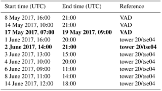
During the IOP, the three DLR long-range lidars were mainly performing continuous vertical scans to capture all flow features over the valley. The experimental scanning with adapting scenarios was only carried out in selected periods with varying westerly to northerly winds of moderate strength. A list of the measurement periods is given in Table 2. For the analysis in this study, two subsets of these periods are picked in which the systems were all working fine and the wind direction showed some variation. Within these times, only cases with free-stream wind speeds larger than 5 m s⁻¹ are used. The first period is from 17 May 2017 at 17:00 UTC until 18 May 2017 at 06:30 UTC, where the wind direction updates were retrieved from VAD scans of lidar #3. The second period is from 2 June 2017 at 16:00 UTC until 2 June at 20:00 UTC, where tower 20/tse04 provided the wind direction updates.

Table 2 List of periods with adaptive multi-Doppler measurements. The column “reference” indicates if wind direction reference was obtained from VAD scans or meteorological tower 20/tse04. In bold are the periods that are looked at in detail in this study.

3 Methods

3.1 Velocity azimuth display

The velocity azimuth display (VAD) method was chosen to determine wind direction and wind speed with lidar #3. The scans were carried out with an elevation angle of φ = 75^∘, an angular speed of 10^∘ s⁻¹ and a range gate distance of 100 m. The calculation of wind speed and wind direction is done through a fit of the curve of radial wind speeds v_r over azimuthal angle θ to Eq. (1):

$$\begin{array}{}\text{(1)}& {\displaystyle }{\displaystyle }{v}_{\mathrm{r}}\left(\mathit{\theta }\right)=a\cos \left(\mathit{\theta }-{\mathit{\theta }}_{\mathrm{0}}\right)+b,\end{array}$$

with a the amplitude of the sinusoidal fit, which translates to horizontal wind speed through u = $\frac{a}{\cos \mathit{\phi }}$, and b its offset, from which vertical wind speed w = $\frac{b}{\sin \mathit{\phi }}$ can be calculated. Wind direction is the phase shift θ₀ of the fit (Newman et al., 2016). The calculation of horizontal wind speed through this method assumes a homogeneous and divergence-free wind field, which is doubtful in the given complex terrain but will be evaluated for the wind direction estimation in this study in Sect. 4.

3.2 Multi-Doppler wind vector calculation

With multiple linearly independent radial wind speed measurements at the same point in space, the meteorological wind vector can be calculated. To calculate the three-dimensional wind vector, at least three independent radial wind speeds are necessary. The relation between meteorological wind vector [u, v, w] and radial wind speeds [v_r1, v_r2, v_r3] can be described as

$$\begin{array}{}\text{(2)}& {\displaystyle }{\displaystyle }\left[\begin{array}{c}{v}_{\mathrm{r}\mathrm{1}}\\ v_{\mathrm{r}\mathrm{2}}\\ v_{\mathrm{r}\mathrm{3}}\end{array}\right]=\left[\begin{array}{ccc}\sin {\mathit{\theta }}_{\mathrm{1}}\cos {\mathit{\phi }}_{\mathrm{1}}& \cos {\mathit{\theta }}_{\mathrm{1}}\cos {\mathit{\phi }}_{\mathrm{1}}& \sin {\mathit{\phi }}_{\mathrm{1}}\\ \sin {\mathit{\theta }}_{\mathrm{2}}\cos {\mathit{\phi }}_{\mathrm{2}}& \cos {\mathit{\theta }}_{\mathrm{2}}\cos {\mathit{\phi }}_{\mathrm{2}}& \sin {\mathit{\phi }}_{\mathrm{2}}\\ \sin {\mathit{\theta }}_{\mathrm{3}}\cos {\mathit{\phi }}_{\mathrm{3}}& \cos {\mathit{\theta }}_{\mathrm{3}}\cos {\mathit{\phi }}_{\mathrm{3}}& \sin {\mathit{\phi }}_{\mathrm{3}}\end{array}\right]\left[\begin{array}{c}u\\ v\\ w\end{array}\right]=\mathit{M}\mathit{u}\end{array}$$

or solved for the meteorological wind vector u:

$$\begin{array}{}\text{(3)}& \mathit{u}={\mathit{M}}^{-\mathrm{1}}{\mathit{v}}_{\mathrm{r}}.\end{array}$$

The uncertainty of the retrieval of the wind velocity component u (and equivalently for v and w) that is introduced by the geometrical arrangement of the lidars can be calculated by propagating the uncertainty of each lidar's radial wind speed uncertainty through Eq. 3:

$$\begin{array}{}\text{(4)}& {\displaystyle }{\displaystyle }{\mathit{ϵ}}_{\mathrm{u}}=\sqrt{\sum _{j=\mathrm{1}}^{\mathrm{3}}{\left({\displaystyle \frac{\partial u}{\partial v_{\mathrm{r},j}}}\right)}^{\mathrm{2}}{\left({\mathit{ϵ}}_j\right)}^{\mathrm{2}}},\end{array}$$

as has for example been described for dual-Doppler applications by Hill et al. (2010). For a common uncertainty ϵ of all lidars, the equation is equivalent to a multiplication of the ℓ² norm of the column vector of M⁻¹ with ϵ and thus equivalent to the method described in Debnath et al. (2017). Pauscher et al. (2016) have shown for the same type of instruments as used in this study (Leosphere Windcube 200S with WindScanner software) that the uncertainty of radial wind speeds is on the order of 0.1 m s⁻¹ when compared to a sonic anemometer. If this value is used as the input uncertainty ϵ for Eq. (4), even the uncertainty of the w component is approximately 1 m s⁻¹ in the sector of interest. It was planned to run the adaptive scanning strategies for wind directions ranging from 240 to 50^∘ in a clockwise direction. For the two analyzed periods, only wind directions between approximately 290 and 360^∘ occurred. Figure 5 shows a color map of the uncertainties at measurement height (hub height) in a radius of 10 rotor diameters around the wind turbine and depicts the target sector and the actual measurement points. It is evident that, in the direction where lidar locations are almost collinear, the uncertainties are extremely high, but in the sector which is relevant for westerly and northwesterly winds, as in the case studies, the uncertainties are lowest. Wildmann et al. (2018) compared radial wind speeds measured in Perdigão with a 100 m mast in the valley. The results of this comparison are on the order of 0.4 m s⁻¹, which is likely due to the very complex flow in that area and the increased uncertainty due to the spatial distance between sonic anemometer and lidar measurement volume in the experimental setup. However, calculating the uncertainty map for this input uncertainty still shows horizontal wind speed component uncertainties below 1 m s⁻¹, and the vertical wind component becomes very uncertain (> 2 m s⁻¹). It is for this reason that analysis in this study has been limited to horizontal wind speeds.

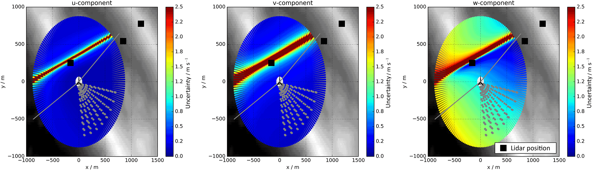
Figure 5 Map of uncertainties at hub height in a radius of 10 D around the wind turbine for the u, v and w component of the wind vector for a radial wind speed uncertainty ϵ = 0.1. The gray lines show the borders of the target sector for wake measurements; the gray dots show the actual measurement points during the two analyzed periods. In the background is the orography in gray scale.

3.3 Wake center estimation

In order to evaluate the displacement of the measurement points from the wake center, wake center positions are determined from single line-of-sight measurements of the three lidars. It is assumed that the wake takes a shape as described in Trujillo et al. (2011), so that single line-of-sight measurements through the wake center will manifest in a Gaussian-shaped velocity profile. Since the line-of-sight measurements have a certain elevation angle, the vertical wind profile is superimposed on the Gaussian profile. Before fitting a Gaussian function as in Eq. (5) to the line-of-sight measurement, it is therefore reduced by the linear trend.

$$\begin{array}{}\text{(5)}& {\displaystyle }{\displaystyle }v\left(x\right)=A_{\mathrm{g}}{e}^{-\frac{{\left(x-b_{\mathrm{g}}\right)}^{\mathrm{2}}}{\mathrm{2}{\mathit{\sigma }}^{\mathrm{2}}}}+d\end{array}$$

A_g is the amplitude of the Gauss-function and σ is the standard deviation. The center of the fitted Gaussian function b_g represents the wake center position projected onto the lidar beam.

3.4 Wake models

To give the measurements some reference, the well-known Jensen–Park model is used in this study according to Jensen (1983) and Peña et al. (2016):

$$\begin{array}{}\text{(6)}& {\displaystyle }{\displaystyle }\mathrm{1}-{\displaystyle \frac{u\left(x\right)}{u_{\mathrm{\infty }}}}={\displaystyle \frac{\mathrm{1}-\sqrt{\mathrm{1}-C_{\mathrm{t}}}}{{\left(\mathrm{1}+k_{\mathrm{w}}\mathrm{2}x/D\right)}^{\mathrm{2}}}},\end{array}$$

with u(x) being the wind speed at distance x to the turbine; C_t being the thrust coefficient of the wind turbine, whose exact value is unknown in this study but assumed to be 0.78; D being the rotor diameter; and u_∞ being the wind speed of the inflow. Assuming that friction velocity u_* is proportional to σ_u, k_w ≈ 0.4I can be assumed (Peña et al., 2016), where I is turbulence intensity and is obtained from sonic anemometer measurements at tower 37/rsw06. Theoretically this relation only holds for flat and homogeneous terrain such as we do not have in Perdigão. Nevertheless we can derive the theoretical wake decay for the wind turbine in flat terrain as a comparison to our measurements.

It is known to the authors that the Jensen–Park model is a very simplified engineering model, and the implied physics cannot be assumed to provide realistic results for the given experiment, but it is a good reference, because it is well known to the community and can be easily reproduced.

4 Results

4.1 VAD scan and mast comparison

To evaluate the accuracy of the wind direction measurements by the VAD scan in complex terrain, the values that were measured in real time and used for the scenario control are compared to 10 min averages of the sonic anemometer at 80 m of tower 20/tse04 in Fig. 6.

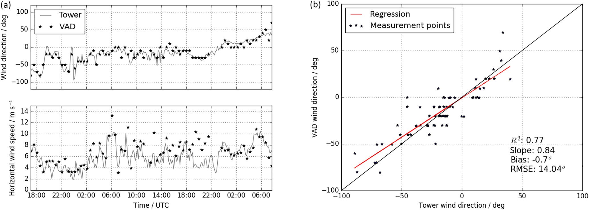
Figure 6 Comparison of lidar #3 VAD scans with sonic anemometer measurements at 80 m on tower 20/tse04 from 17 to 19 May. (a) Comparison of the time series of wind direction and wind speed, and (b) a regression plot of wind directions.

It shows that wind direction trends agree well, but differences of up to 10–20^∘ can be observed, with a root mean squared error of 14.04^∘. The estimation of horizontal wind speed shows larger differences, especially during daytime, which is likely due to convection and a vertical wind component that cannot be neglected and leads to an overestimation of the VAD measurement.

4.2 Synchronization accuracy

For the purpose of crossing beams of multiple lidars at the same point in time and space, high demands are made on the pointing and timing accuracy of each system. In Vasiljevic (2014) it is explained in detail how hard-target calibration of the pointing direction can be done, and how the timing synchronization based on a precise GPS clock and synchronization commands of the master computer is realized in the WindScanner system. The accuracy of the hard-target calibration of the azimuth and elevation angle offsets is dependent on the accuracy of the location measurement of the lidars and the targets. For the DLR lidars in the Perdigão 2017 campaign, locations were first measured with a single-frequency GPS receiver in precise-point-positioning (PPP) mode, which allows accuracies on the order of 1–2 m. After 3 weeks of the campaign, a dual-frequency GPS receiver with centimeter accuracy was available, and calibration was repeated. It was found that the offsets with the more accurate location measurement differed by up to 0.6^∘ from the original calibration. This error is not uniquely due to the wrong position measurement, but it is also due to maladjustment because of slight movements of the lidar on non-solid ground. An error of 0.6^∘ for lidar #1 leads to a spatial offset of the measurement point of approximately 15 m at the location of the wind turbine and has to be taken into account. The error is, however, of the same magnitude as the physical resolution of the lidar, so it is considered acceptable for further analysis. The large error applies to the measurements from 17 to 19 May. Measurements on 2 June were done with the more accurate readjustment.

Usually, the WindScanner software allows timing synchronization down to 10 ms of all systems, which was demonstrated in a number of campaigns with a development version of the software (Vasiljevic et al., 2016). Because of a bug in the commercial version of the WCS that miscalculated scanner movement times depending on the acceleration and deceleration periods, timing was less accurate in the presented experiment. Figure 7 shows the time difference between the three systems for each measurement point in a 2 h period on 2 June. It shows that the standard deviation of the timing errors mostly stays below 0.2 s, which is an acceptable error for the given experiment concerning mean wind speeds, but it is critical to have better accuracy for turbulence measurements.

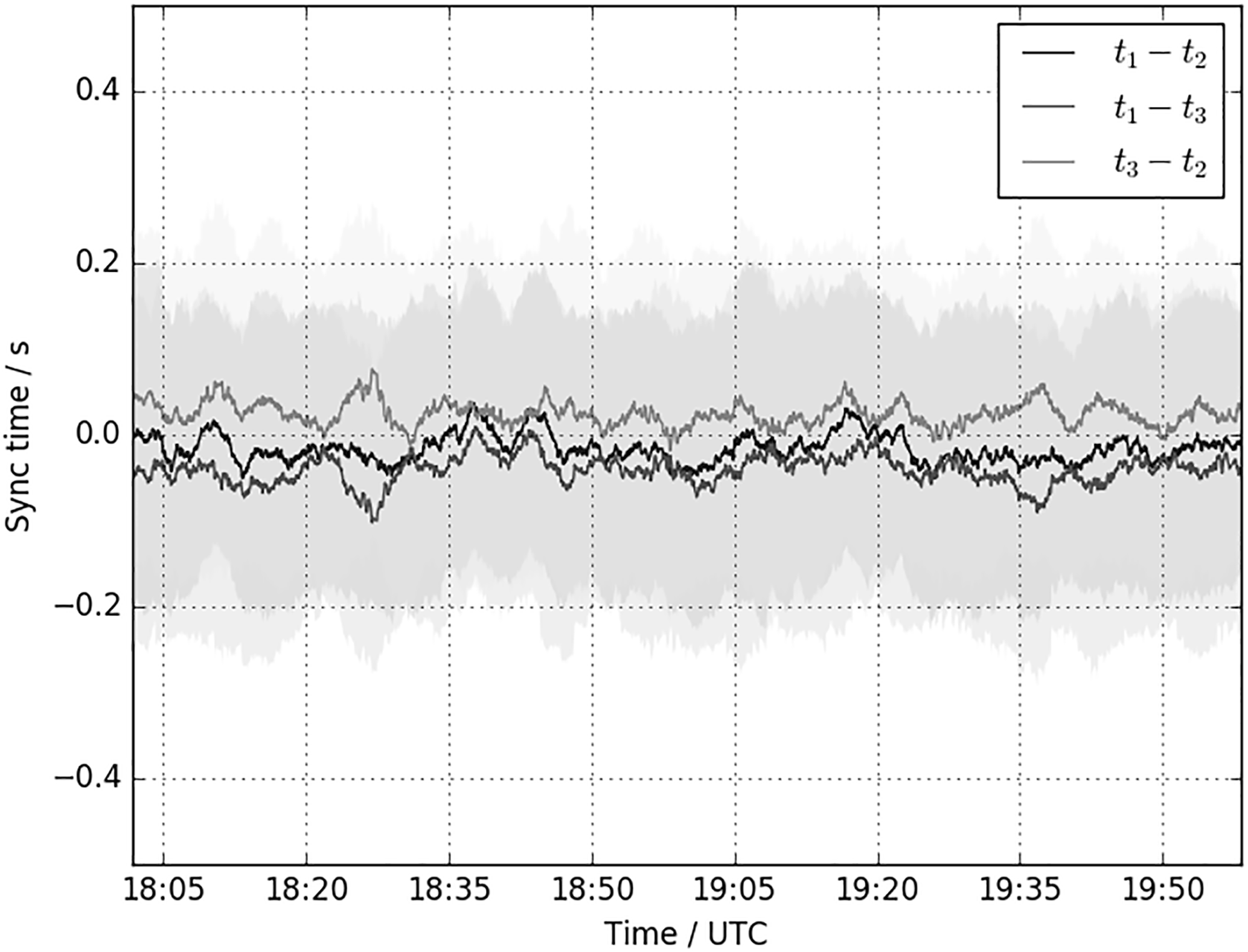
Figure 7 Time difference between lidar #1 (t₁), lidar #2 (t₂) and lidar #3 (t₃) for an exemplary period on 2 June. The lines show the moving average synchronization error over 100 scanning points, and the shaded area is the standard deviation.

4.3 Wake measurements

4.3.1 Wind speed deficit

With the described measurement strategy, wind speed deficits can be calculated downstream of the turbine in the main wind direction in relation to the distance to the rotor. Figures 8 and 9 show the results as horizontal wind speed measurement and wind speed deficit, normalized to the upstream wind speed v_∞ for the 2 days of interest. For all cases, v_∞ is the extrapolated wind speed at hub height from measurements of the upstream tower 37/rsw06, with sonic anemometer measurements up to 60 m. For the analysis, only 30 min averages with inflow wind speeds of more than 5 m s⁻¹ are used.

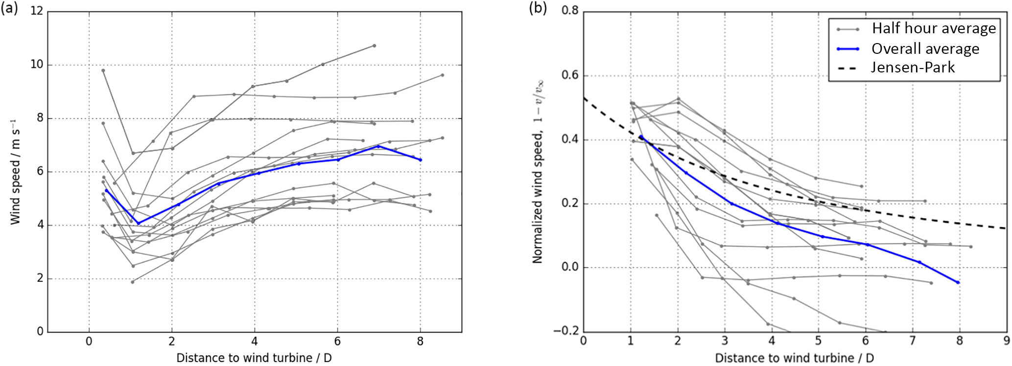
Figure 8 Multi-Doppler wind speed measurements plotted against distance to the turbine (a), and wind speed deficit normalized to undisturbed wind speed measurement on tower 20/tse04 at 80 m (b) on 17 May 2017.

Figure 9 Multi-Doppler wind speed measurements plotted against distance to the turbine (a), and wind speed deficit normalized to a measurement point 1 rotor diameter upstream (b) on 2 June 2017.

The results show that there is a large spread in the measured wind speed deficits. On average, for the observed periods, the decay of the wake is similar to what the Jensen–Park model describes for flat and homogeneous terrain. Some of the 30 min averages show a fast decay of the wind speed deficit, especially on 17 May. In these cases, the alignment of the measurement points with the wake center was too far off, which has the effect that measurement points at far distances to the wind turbine are outside the wake, and thus the wind speed deficit gets small and no longer represents the wake. This situation will be evaluated in Sect. 4.3.3.

4.3.2 Turbulence intensity

As described in Sect. 4.2, movement of the scanners between measurement points in this study was limited in speed. The sampling rate at every measurement point is only about 1∕20 s which means that at a mean wind speed of 5 m s⁻¹ and according to the Nyquist theorem, only eddies larger than 240 m are sampled. Given these constraints, it is possible to calculate turbulence intensity at the triple-Doppler measurement points as I = $\frac{{\mathit{\sigma }}_{\mathrm{u}}}{\stackrel{\mathrm{‾}}{u}}$. Figure 10 shows the result of this analysis in comparison to measurements at tower 37/rsw06 for the sonic anemometer at 60 m. The sonic anemometer turbulence intensity is calculated in the same way, but standard deviation and mean value are calculated for 10 min periods with a sampling rate of 20 Hz. It shows that, in close proximity to the wind turbine, I is twice as high as in the undisturbed atmosphere, but at 8 D downstream it is back to the background level in almost all cases.

Figure 10 Turbulence intensity plotted against distance to the wind turbine for half-hour periods (gray lines) and overall average (blue line) on 17 May 2017 (a) and 2 June 2017 (b). The red line shows the average turbulence intensity for the observed period on tower 37/rsw06, and the red area is the area between maximum and minimum turbulence intensity in the period.

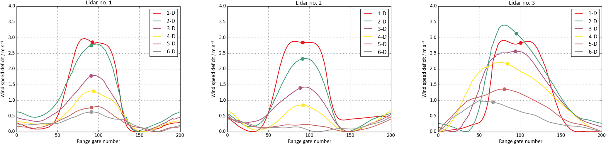
Figure 11 Averaged line-of-sight measurements through the wake by the three lidar systems at different distances to the wind turbine. The dots show the estimated wake center positions by a Gaussian fit.

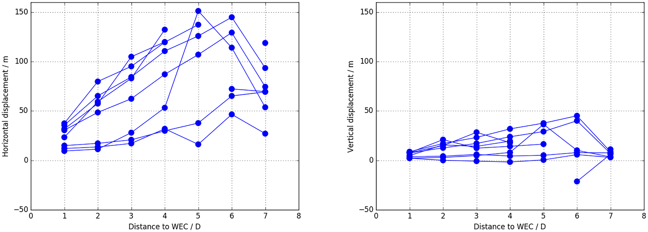
Figure 12 Averaged misalignment of the determined wake center to the beam-crossing measurement point.

4.3.3 Wake center position

With additional range gates before and after the crossing point of the lidar beams, a spatial resolution of the wake shape and its center position can be achieved. On 17 May, the extra range gates were only placed 50 m before and behind the lidar-beam-crossing point, with a resolution of 1 m. This proved not to be enough for a proper fit of a theoretical wake profile to the data. In later measurements, as on 2 June, range gates were placed 200 m before and behind the crossing point with a resolution of 2 m.

Figure 11 shows averaged line-of-sight measurements through the wake for one half-hour period. For lidars #1 and #2 the estimated wake center is quite close to the center of the range gate (although never perfectly matching it) with a trend of a bigger displacement with increasing distance to the wind turbine. For lidar #3 the mismatch is very obvious, because this lidar cuts the wake with the highest elevation angle, whereas the wake flow follows the terrain downslope, and the wake center appears in range gates closer to the lidar than the center range gate.

The misalignment error can be quantified as the mismatch between estimated wake center position and the position where the lidar beams cross, as depicted for each half-hour measurement period against the distance to the turbine in Fig. 12. The offset is obviously large and should be reduced in future experiments by a better prediction of the wake center, taking into account the wind turbine yaw angle if possible and reducing the update cycle to less than 30 min.

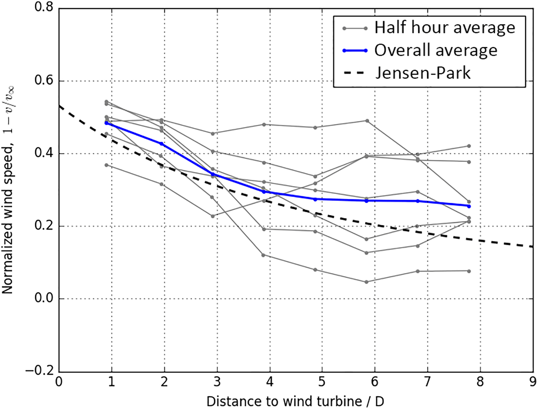
Figure 13 Wind speed deficit behind the wind turbine when using minimal wind speeds of line-of-sight measurements of the three lidars for wind speed retrieval.

If, instead of the wind speeds at the lidar-beam-crossing point, the minimum wind speeds of the 400 m long range with measurement points along the line of sights of the lidar beams are used for the wind speed retrieval on 2 June, a larger wind speed deficit is found (see Fig. 13). Of course, this will also not be the real wind speed deficit in the center of the wake, because not all three beams cut the wake at its center.

5 Conclusions

With this study it is shown for the first time that long-range lidar systems – upgraded with the WindScanner software – can be used in a flexible way with automatically adjusting scanning trajectories. In the context of wind turbine wake measurements this technology is a powerful tool because it enables continuous monitoring of the wake in a multi-Doppler mode with ground-based lidars, whereas a static configuration is only able to provide wake data in short periods of time. The measurement results are confronted with the theoretical wake decay as it is calculated with the Jensen–Park model. Although a good agreement cannot be assumed given the complex terrain and non-neutral stratification of the atmosphere during the observed periods, the averaged measured wind speed deficit is close to the model prediction. The spread is large, which can be attributed not only to the complex flow but also to remaining uncertainties in the measurement strategy. Despite rather slow sampling times, it could be shown that, with the measurement strategy, the increased turbulence intensity in the wake can be measured and quantified.

In 10 measurement periods, the method has been tested and developed. A number of lessons learned are given here to summarize the potential and limitations of the technique:

• The lidar locations were chosen for a different scanning strategy and were not optimized to cover the full span of wind directions. In future experiments lidar locations should be optimized to obtain lowest uncertainties in all dominant wind directions.

• The slow synchronization that has been described in Sect. 4.2 has already been fixed in the WindScanner software. In future experiments it will thus be possible to scan much faster, achieving higher temporal resolutions and better synchronization of the lidars, which will hence allow the resolution of turbulence statistics to scales as small as the physical resolution of the instruments.

• The wind directions used for the scan adaptation in this study were first based on VAD scans of one of the lidars and later on sonic anemometer measurements of a tower close to the wind turbine. It is shown that both strategies work in general, but using an external source for the wind direction increases the availability. Especially in complex terrain, VAD scans have significant errors compared to sonic anemometer measurements. The combination of tower data and lidar measurements is a good example of a “smart” experimental setup, which in this case was possible because of the extraordinary infrastructure in Perdigão. In experiments with less infrastructure and less complex terrain, the VAD method can still be a good alternative. Higher update rates than the 30 min that were used in this experiment are necessary if wind conditions and yaw angle of the wind turbine change as quickly as they did in Perdigão.

• Large improvements are expected if the wind direction measurement of the wind turbine itself, or even better its measured yaw angle, could be used for control of the lidars. Another option would be to track the wake in real time and use this information for control of lidar scans, but this would require more independent instrumentation.

• A reduction of the time for reconfiguration of the scanning trajectories will further increase the data availability.

• Since the wake will always deviate slightly from the predicted location, multiple range gates before and after the determined center position for each line-of-sight measurement are helpful to determine the wake center in post-processing and also allow some analysis of wake widths. The range gates should be close to each other, but the range should also be large enough to cover the whole width of the wake and allow automatic wake center detection with suitable fitting functions. Range gates 200 m (or 2.5 rotor diameters) before and behind the determined range gate center, with a separation of 2 m, have proven to be suitable for the given wind turbine.

• An extra measurement point should be set at a minimum of 2.5 rotor diameters upstream for a better estimation of the free-stream velocity v_∞.

A next step towards better understanding of wake dynamics is to apply the lessons learned from this case study to a long-term campaign which focuses on this measurement strategy and will allow better statistics of the wake characteristics to be obtained in different atmospheric conditions. Currently, a research wind park is being planned in northern Germany by the DLR and its partners which will be equipped with scientific instrumentation on all levels from rotor blade, nacelle, tower and foundation to the atmosphere in near and far field, including the systems presented in this study. It is evident that this facility will be an ideal platform for performing dedicated experiments in flat terrain in order to get more basic understanding of wake physics without the effects induced by complex terrain. With the dataset that was obtained in the Perdigão 2017 experiment, a good basis for research in the field of interaction of a wind turbine with the atmosphere in complex terrain is given. In the future, numerical models on different scales will need to be compared to and validated with the dataset.