the Creative Commons Attribution 4.0 License.
the Creative Commons Attribution 4.0 License.
 | 17 Jan 2018
GOCI Yonsei aerosol retrieval version 2 products: an improved algorithm and error analysis with uncertainty estimation from 5-year validation over East Asia
Myungje Choi
Jaehwa Lee
Mijin Kim
Young-Je Park
Brent Holben
Thomas F. Eck
Zhengqiang Li
Chul H. Song
The Geostationary Ocean Color Imager (GOCI) Yonsei aerosol retrieval (YAER) version 1 algorithm was developed to retrieve hourly aerosol optical depth at 550 nm (AOD) and other subsidiary aerosol optical properties over East Asia. The GOCI YAER AOD had accuracy comparable to ground-based and other satellite-based observations but still had errors because of uncertainties in surface reflectance and simple cloud masking. In addition, near-real-time (NRT) processing was not possible because a monthly database for each year encompassing the day of retrieval was required for the determination of surface reflectance. This study describes the improved GOCI YAER algorithm version 2 (V2) for NRT processing with improved accuracy based on updates to the cloud-masking and surface-reflectance calculations using a multi-year Rayleigh-corrected reflectance and wind speed database, and inversion channels for surface conditions. The improved GOCI AOD τG is closer to that of the Moderate Resolution Imaging Spectroradiometer (MODIS) and Visible Infrared Imaging Radiometer Suite (VIIRS) AOD than was the case for AOD from the YAER V1 algorithm. The V2 τG has a lower median bias and higher ratio within the MODIS expected error range (0.60 for land and 0.71 for ocean) compared with V1 (0.49 for land and 0.62 for ocean) in a validation test against Aerosol Robotic Network (AERONET) AOD τA from 2011 to 2016. A validation using the Sun-Sky Radiometer Observation Network (SONET) over China shows similar results. The bias of error (τG−τA) is within −0.1 and 0.1, and it is a function of AERONET AOD and Ångström exponent (AE), scattering angle, normalized difference vegetation index (NDVI), cloud fraction and homogeneity of retrieved AOD, and observation time, month, and year. In addition, the diagnostic and prognostic expected error (PEE) of τG are estimated. The estimated PEE of GOCI V2 AOD is well correlated with the actual error over East Asia, and the GOCI V2 AOD over South Korea has a higher ratio within PEE than that over China and Japan.
- Article
(11153 KB) - Full-text XML
- Companion paper
- BibTeX
- EndNote


Aerosols are one of the most important components in the atmosphere with respect to climate change and air pollution. Aerosols influence the climate directly by scattering and absorbing solar radiance (aerosol–radiation interactions) and indirectly by altering cloud properties (aerosol–cloud interaction; IPCC, 2013). Two aerosol optical properties (AOPs), the aerosol optical depth and single-scattering albedo, determine the sign and magnitude of the shortwave aerosol radiative forcing of the atmosphere for different surface conditions (Takemura et al., 2002). Thus, accurate AOP retrievals are important for quantifying the role of aerosols in climate change. With respect to air pollution, ambient fine particulate matter (PM) affects respiratory and pulmonary systems, resulting in an increased incidence of heart disease, strokes, and lung cancer (Lim et al., 2012). While PM information is often obtained from ground-based in situ measurements, the coverage of ground-based measurements is limited to the local scale and observational networks are often sparse, especially in developing countries. However, satellite-based remote sensing can provide aerosol information over a much broader area. Chemical transport models (CTMs) make many assumptions in predictions of PM concentrations. Modeling accuracy can be improved significantly through data assimilation with satellite-retrieved aerosol optical depth (AOD) products (van Donkelaar et al., 2010).
East Asia has some of the highest aerosol concentrations in the world, with components that include desert dust, anthropogenic carbonaceous aerosols, and sea salt (Kim et al., 2007; Yoon et al., 2014). Trends in aerosol concentrations in East Asia do not show the same significant decreases seen in Europe or North America (Zhang and Reid, 2010; Hsu et al., 2012), for reasons that are still unclear (IPCC, 2013).
The Geostationary Ocean Color Imager (GOCI), launched in 2010 as the first ocean color imager in geostationary orbit (GEO), observes East Asia eight times per day from 00:30 to 07:30 Coordinated Universal Time (UTC; 09:30 to 16:30 Korea Standard Time (KST); Choi et al., 2012). Using the radiance measurements from eight spectral channels (412, 443, 490, 555, 660, 680, 745, and 865 nm) with high spatial resolution (500 m × 500 m), the GOCI Yonsei aerosol retrieval (YAER) version 1 (V1) algorithm was developed to retrieve hourly aerosol optical properties such as aerosol optical depth (AOD) with simple diagnostic parameters such as fine-mode fraction (FMF), Ångström exponent (AE), and single-scattering albedo (SSA; Choi et al., 2016). Because it has more channels with higher spatial resolution in the visible and near-infrared (NIR) bands compared with recent and planned advanced meteorological sensors in GEO, including the Advanced Himawari Imager (AHI), the Advanced Baseline Imager (ABI), and the Advanced Meteorological Imager (AMI), GOCI provides valuable information related to AOPs. Hourly AOD from the GOCI YAER algorithm is in good agreement with Moderate Resolution Imaging Spectroradiometer (MODIS) and Visible Infrared Imaging Radiometer Suite (VIIRS) AOD over East Asia (Xiao et al., 2016). The application of GOCI retrievals through data assimilation results in improved performance of several air quality forecasting model predictions of AOD and PM concentrations (Park et al., 2014; Saide et al., 2014; Jeon et al., 2016; Lee et al., 2016; Lee et al., 2017). For this reason, a need has arisen for GOCI aerosol retrievals with near-real-time (NRT) processing for operational air quality forecasting systems using data assimilation.
The lack of shortwave infrared (SWIR) channels in GOCI (similar to the 1.6 or 2.1 µm channels of MODIS) does not allow for the calculation of surface reflectance in the visible range from top-of-atmosphere (TOA) reflectance in the SWIR range (Kaufman et al., 1997). Instead, the minimum reflectivity technique using the composite method (Herman and Celarier, 1997; Koelemeijer et al., 2003; Hsu et al., 2004) was applied in the GOCI YAER V1 algorithm. However, this methodology prevents the GOCI YAER V1 algorithm from being capable of near-real-time (NRT) processing because it required a monthly database for each year encompassing the day of retrieval for the determination of surface reflectance. In addition, the resulting retrievals have a slightly negative bias over land and a positive bias over ocean due to surface reflectance errors, compared with AERONET data during the Distributed Regional Aerosol Gridded Observation Networks – Northeast Asia 2012 campaign (DRAGON-NE Asia 2012 campaign; Choi et al., 2016).
In this study, version 2 (V2) of the algorithm is developed to both allow NRT processing and improve accuracy. Monthly and hourly surface reflectance and wind speed determinations are modified using a climatological database from the multi-year GOCI dataset and reanalysis wind speed data, respectively. The surface reflectance database obtained from multi-year Rayleigh-corrected reflectance (RCR) samples enables more accurate surface reflectance retrievals by increasing the availability of measurements that are not aerosol- or cloud-contaminated, compared with the 1-year samples of the V1 algorithm. The cloud masking and inversion spectral channels for aerosol retrievals were also modified for better accuracy. Furthermore, retrieved GOCI YAER V2 AOD is evaluated using ground-based observation data, along with comparisons with both V1 and MODIS retrievals from March 2011 to February 2016, which is a longer evaluation period than used in previous studies. The bias of the GOCI YAER V2 AOD is analyzed and uncertainties are estimated to facilitate the application of GOCI AOD in data assimilation.
The remainder of this paper is organized as follows. In Sect. 2, improvements in the GOCI YAER V2 algorithm are summarized and a quantitative comparison with other satellite AODs is presented. In Sect. 3, the GOCI YAER V2 AOD is validated using ground-based sun-photometer observations along with other satellite AOD measurements. In Sect. 4, GOCI YAER V2 AOD errors are analyzed in relation to various parameters and expected errors are estimated. Finally, a summary and conclusions are presented in Sect. 5.
2.1 Overview of the GOCI YAER V1 and V2 algorithm framework
A prototype of the GOCI YAER algorithm for use over the ocean (Lee et al., 2010) was developed using MODIS Level 1B (L1B) top-of-atmosphere (TOA) reflected radiance data and improved using nonspherical AOPs (Lee et al., 2012). Then, using real GOCI L1B TOA radiance data, the GOCI YAER V1 algorithm for use over land and ocean surfaces was developed (Choi et al., 2016). The algorithm is applied to cloud-free and snow/ice-free pixels. Sets of 12 pixel × 12 pixel blocks are aggregated to achieve 6 km × 6 km spatial resolution and averaged after cloud/snow/ice masking and suitable pixel selection.
Unified aerosol models over land and ocean surfaces classify aerosols using AOD at 550 nm, FMF at 550 nm, and SSA at 440 nm derived from the global Aerosol Robotic Network (AERONET) inversion database (Dubovik and King, 2000; Holben et al., 1998). This aerosol type classification (Lee et al., 2012) covers a range of AOPs: FMF from 0.1 to 1.0 at an interval of 0.1 and SSA from 0.85 to 1.00 at an interval of 0.05. A total of 26 aerosol models are assumed in the algorithm: nine highly absorbing, nine moderately absorbing, and eight nonabsorbing models. Note that AOPs to calculate AOD are constructed to account for hygroscopic growth and aggregation (Eck et al., 2003; Reid et al., 1998). Non-spherical properties are considered using the phase function derived from AERONET data.
Dark ocean surface reflectance is calculated using the Cox–Munk model (Cox and Munk, 1954) considering Fresnel reflectance with a bidirectional reflectance distribution function according to geometry and wind speed in a precalculated look-up table (LUT) with temporal interpolation of ECMWF wind speed data at 10 m above sea level (m a.s.l.) over dark ocean pixels (Dee et al., 2011). Land surface reflectance is obtained using the minimum reflectivity technique for each month, channel, and hour, and temporal interpolation is carried out over land, turbid ocean, and heavy aerosol pixels in the inversion step. In the algorithm, turbid water pixel detection is implemented using a difference of 660 nm TOA reflectance between directly observed and interpolated data from 412 and 865 nm (hereafter, Δρ660; Li et al., 2003; Choi et al., 2016).
All eight channels are used over ocean surfaces, and different combinations of channels are used over land, depending on surface conditions. Measured spectral TOA reflectance can be converted to spectral AOD for all aerosol models using the precalculated LUT, and spectral AOD can be converted to the corresponding value at 550 nm using the assumed AE of each aerosol model. Then, the mean value and standard deviation (SD) of AOD at 550 nm from different channels are calculated for each aerosol model, and the three aerosol models with the lowest SD are selected. The SD-weighted average of mean AOD at 550 nm from the three selected aerosol models is used as the AOD at 550 nm. An identical SD-weighted average is applied to the assumed AE, FMF, and SSA of the selected aerosol models to determine the final AE, FMF, and SSA values. This inversion method is focused primarily on the retrieval of AOD at 550 nm from multi-channel spectral information, and the AE, FMF, and SSA are determined from aerosol models selected for the best AOD fit. Thus, AOD at 550 nm is the main retrieval product, and the AE, FMF, and SSA are considered as diagnostic parameters, or ancillary products. Note that the discrete ordinate radiative transfer (DISORT) code of the libRadtran software package is used to calculate TOA reflectance for the LUT construction based on scalar calculations (i.e., intensity-only) and a plane-parallel atmosphere approximation (Mayer and Kylling, 2005).
To improve the accuracy of AOP retrieval from GOCI measurements, AOD in particular, the new V2 algorithm is developed through piecewise upgrades to the V1 algorithm while retaining the structure and conceptual approach of the original algorithm. A flow chart of the GOCI YAER V2 algorithm is presented in Fig. 1. The improved parts of the V2 algorithm compared with V1 are the pixel masking and aggregation procedures, implementation of the climatological surface reflectance and wind speed from a 5-year climatological database for NRT calculations, turbid water detection, and inversion conditions for land, turbid water, and dark ocean pixels. The aerosol model construction and inversion method for converting TOA reflectance to aerosol products are identical to those of V1. Details of the refined parts of the algorithm are introduced in the following subsections.
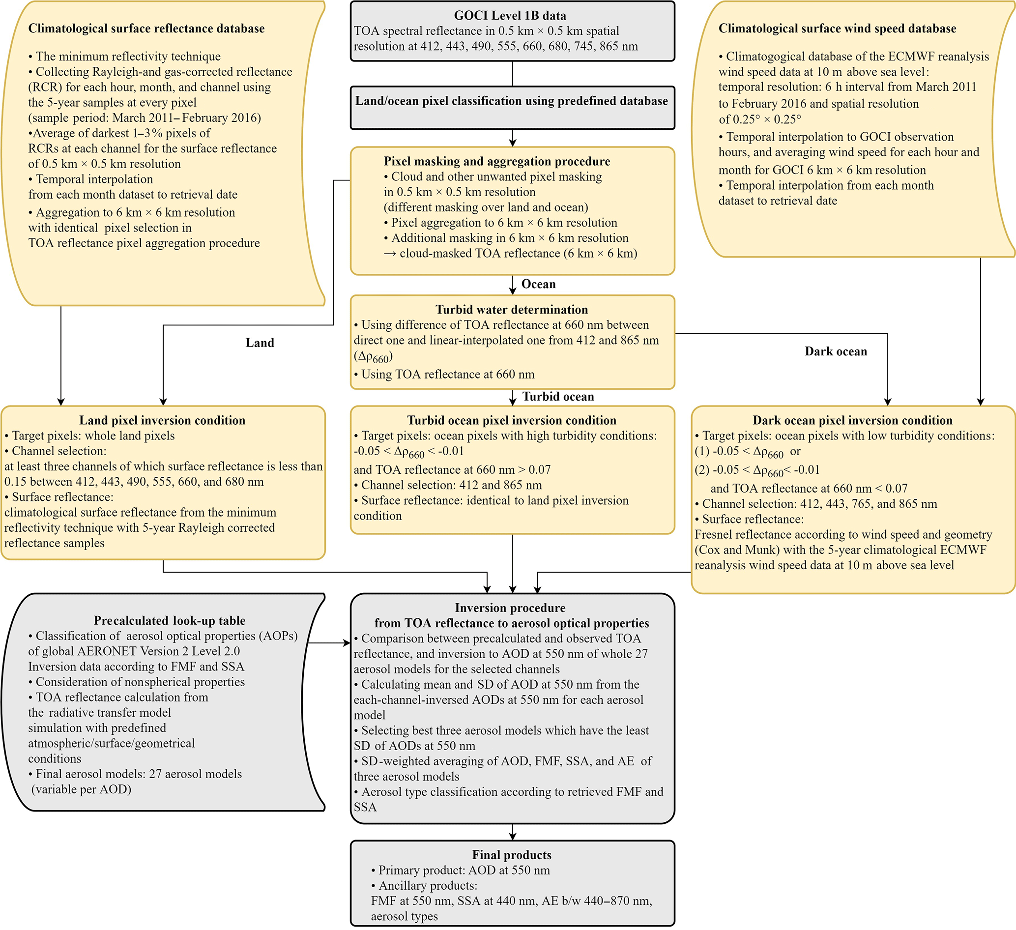
Figure 1Flow chart of the GOCI Yonsei aerosol retrieval version 2 algorithm. Yellow indicates improvements from version 1 to version 2, and gray indicates no change from version 1.
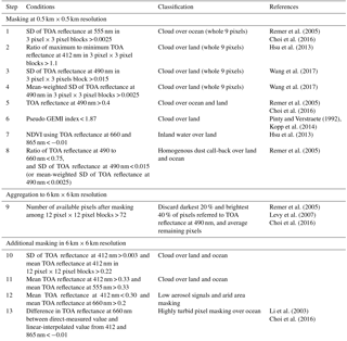
Table 1Cloud and other pixel masking steps of the GOCI YAER V2 algorithm.
2.2 Pixel masking and aggregation procedure
The GOCI YAER algorithm is targeted to cloud-free and snow-free pixels over land and cloud-free, ice-free, and high-turbidity-water-free pixels over the ocean. Therefore, several masking steps are required. The previous V1 algorithm contains simple cloud-masking techniques, which include a spatial variability test using the SD over a 3 pixel × 3 pixel block and a threshold for high TOA reflectance. These simple techniques remove most cloud pixels, but some thin homogeneous (e.g., cirrus) cloud pixels remain because of the absence of ice-crystal-sensitive 1.38 µm or other infrared channels in GOCI. This leads to unfiltered cloud pixels being misclassified as high-AOD pixels and raises the need for additional filtering for successful data assimilation between models and GOCI AOD (Xu et al., 2015). In addition, some low-AOD pixels could be misclassified as cloud pixels in regions with highly inhomogeneous surface reflectance. In this study, therefore, refined cloud-masking techniques are applied, as summarized (with references) in Table 1. Most of these masking techniques were adopted from the MODIS and VIIRS aerosol retrieval and cloud-masking algorithms. The masking procedures consist of three stages: masking at the original 0.5 km × 0.5 km L1B pixel resolution, aggregation from 0.5 km × 0.5 km to 6 km × 6 km resolution, and additional masking at the 6 km × 6 km resolution.
At the 0.5 km × 0.5 km resolution, cloud masking over ocean surfaces is unchanged, but the land-surface cloud-masking steps are refined. The previous SD test of a 3 pixel × 3 pixel block over land for identifying clouds and aerosols (Step 3 in Table 1, except for a threshold of 0.0025) works well for moderate- and high-AOD cases, but it over-masks heterogeneous surface reflectance pixels under low-AOD conditions. Thus, the threshold is relaxed to 0.015, and the mean-weighted SD test (Step 4 in Table 1) and the ratio of maximum to minimum TOA reflectance at 412 nm within the 3 pixel × 3 pixel grid are adopted (Step 2 in Table 1) as an alternative. To identify aerosols and clouds using a different technique, a pseudo Global Environment Monitoring Index (GEMI), developed by Pinty and Verstraete (1992) and Kopp et al. (2014) and applied in the operational VIIRS cloud-mask algorithm (Godin, 2014), is adopted (Step 6 in Table 1). The GEMI is based on the reflectance ratio between 865 and 660 nm and is defined as follows:
where
Note that Ref660 and Ref865 are the TOA reflectance at 660 and 865 nm, respectively. In addition, inland water pixels are filtered out using a normalized difference vegetation index (NDVI) calculated using the TOA reflectance at 660 and 865 nm (Step 7 in Table 1). A dust call-back test used for ocean pixels is expanded to include both ocean and land pixels and is coupled with a spatial homogeneity test (Step 8 in Table 1).
After masking at the 0.5 km × 0.5 km resolution level, the remaining pixels are aggregated to the Level 2 product resolution of 6 km × 6 km. The TOA reflectance of the remaining pixels is averaged if the number of remaining pixels is greater than 72 (Step 9 in Table 1). In this step, the darkest 20 % and brightest 40 % of pixels are discarded to filter out cloud shadow, remaining cloud, and surface contamination, following Choi et al. (2016). The quality assurance (QA) value of the V1 algorithm was determined based on the range of retrieved AOD and the remaining number of pixels in a 12 pixel × 12 pixel block after all masking procedures were performed. A QA value of 0, 1, 2, or 3 for the V1 AOD was assigned for 6, 15, 22, or 36 remaining pixels, respectively. In addition, retrieved AOD values between −0.05 and 3.6 were assigned a QA value of 1, 2, or 3, and retrieved AOD values between −0.1 and −0.05 or between 3.6 and 5.0 were assigned a QA value of 0. The lower of these two QA values for each pixel was used as the final QA value. In the V2 algorithm, however, the retrieval is implemented if the number of remaining pixels is greater than 28, and the QA classification is eliminated. In addition, only pixels with retrieved AOD between −0.05 and 3.6 are included in the calculations. Small negative AOD values can be caused by surface reflectance errors in this algorithm. These are assumed to fall within the range of expected retrieval errors and are statistically significant under low-AOD conditions when compared with results from the MODIS DT algorithm (Levy et al., 2007, 2013). The threshold of maximum AOD of 3.6 is based on Lee et al. (2012), who considered the probability distribution of AOD in the region.
After the pixel aggregation procedure, merged TOA reflectance at the 6 km × 6 km resolution is filtered again. Bright and inhomogeneous pixels within a 12 pixel × 12 pixel block are filtered using the mean and SD at 412 nm (Step 10 in Table 1), and pixels with high TOA reflectance at both 412 and 660 nm are also filtered out (Step 11 in Table 1). Furthermore, pixels with low atmospheric signal (dark at 412 nm) but high surface signal (bright at 660 nm), such as in arid areas, are also filtered out to avoid misidentification of the bright surface signal as aerosol (Step 12 in Table 1).
2.3 Climatological land surface reflectance database from multi-year samples
In the GOCI YAER algorithm, surface reflectance over land is handled differently to that over ocean. A minimum reflectance technique to determine the surface reflectance from the composite Rayleigh-corrected reflectance (RCR) for each month and hour is applied over all land and turbid-water pixels in the V1 algorithm. The GOCI YAER V1 algorithm was not capable of NRT processing because it required an adjacent 2-month database encompassing the day of retrieval for the determination of surface reflectance.
To achieve NRT retrieval in the V2 algorithm, climatological land-surface reflectance for each channel, hour, and month are calculated over the 5-year period from March 2011 to February 2016. The V1 surface reflectance database was calculated at a 6 km × 6 km resolution by the aggregation of 12 pixel × 12 pixel data to extend the number of RCR samples. The V1 surface reflectance calculation assumes that surface reflectance within a 6 km × 6 km area is homogeneous. The V1 surface reflectance calculation resulted in slightly negatively biased AOD at low AOD over South Korea and Japan during spring 2012, which means that the surface reflectance was overestimated (Choi et al., 2016). In the V2 algorithm, temporal RCR samples are expanded from a 1-year period to a 5-year period, thereby improving performance under low aerosol conditions and reducing the negative bias in reflectance of the V1 algorithm. The spatial resolution of climatological land surface reflectance used in the V2 algorithm is 0.5 km × 0.5 km for the L1B TOA reflectance, an improvement over the 6 km × 6 km resolution used in the V1 algorithm. This higher resolution can capture highly spatially variable surface reflectance and improve the identical pixel matching between TOA and surface reflectance during pixel aggregation. The maximum number of composite 5-year RCR samples used to determine the surface reflectance of a single pixel is 155 (31 days × 5 years). The darkest samples (the lowest 0–1 % of the aggregate sample) are assumed to be cloud shadow and the brightest samples (3–100 % of the aggregate sample) are assumed to be affected by aerosols and/or clouds. Thus, the darkest 1–3 % of the RCR samples are averaged and used to determine surface reflectance, as in the V1 algorithm. According to Hsu et al. (2004), surface reflectance can be obtained by finding the minimum RCR for each month, which corresponds to ∼ 3 % of the aggregate sample. The darkest 0–1 % of pixels are assumed, based on empirical grounds, to be cloud shadow and are thus excluded. This composite procedure is implemented for each month, hour, and channel. Monthly surface reflectance climatological data correspond to the middle of each month (day 15) and are linearly interpolated to the retrieval date. Major year-to-year land use changes over the 5-year period would result in an artificial AOD bias and should be addressed in future work.
2.4 Climatological ocean surface wind speed database from multi-year samples
To calculate dark ocean surface reflectance, the GOCI YAER V1 algorithm uses the ECMWF wind speed at 10 m a.s.l. from reanalysis data, which has a 6 h temporal resolution and 0.25∘ × 0.25∘ spatial resolution. The ECMWF data are interpolated to hourly resolution for use with observations. In the V2 algorithm, the wind speed from a 5-year average of climatological data is used. The wind speed from 5 years of data for each month, hour, and 0.25∘ × 0.25∘ area is averaged. This approach captures seasonal effects, such as higher (lower) wind speeds in winter (summer), and variations in the spatial distribution of wind speed, such as the higher (lower) wind speed in the open sea (coast). As in the land surface reflectance calculations, climatological wind speed data for each month correspond to the middle of each month (day 15) and are linearly interpolated to the retrieval date.
2.5 Refined pixel allocation for the land, turbid water, and dark ocean algorithms and inversion conditions
The GOCI YAER V1 land algorithm is applied not only over land pixels but also over highly turbid or high-AOD ocean pixels; the ocean algorithm is applied only over dark ocean surface pixels. A pixel with Δρ660 below −0.05 is assumed to be dark ocean and is processed using the dark ocean algorithm. Pixels with Δρ660 between −0.05 and −0.01 are classified as turbid water and thus use the land algorithm. Pixels with Δρ660 above −0.01 are assumed to be highly turbid water and removed (Step 13 in Table 1). In some cases, ocean pixels have Δρ660 above −0.05 with extremely low TOA reflectance which could result from a combination of low aerosol concentrations and dark ocean surface reflectance. Misidentification of these pixels as turbid water results in negative AOD over the dark ocean. Therefore, a threshold test to identify extremely dark ocean pixels using TOA reflectance at 660 nm is included in the V2 algorithm. The dark ocean algorithm is applied to pixels with Δρ660 between −0.05 and −0.01 and TOA reflectance at 660 nm of below 0.07.
The channels selected for the inversion from measured reflectance to aerosol optical properties are different for land, turbid water, and dark ocean pixels. In the V1 algorithm, the land and turbid water pixels use channels between 412 and 680 nm with surface reflectance less than 0.15, and the dark ocean pixels use all eight channels. In the V2 algorithm, the channels used for land pixels are the same as in the V1 algorithm, but the channels selected for turbid water and dark ocean pixels have been changed. In the atmospheric correction for ocean color retrieval, the main assumption is that water-leaving radiance is close to zero in the NIR range, and thus NIR bands are used for estimating aerosol loading in the atmosphere. The aerosol signal in the visible range is estimated from NIR measurements and the known relationships of aerosol signals in the visible and NIR range for various aerosol types. Ocean color in the visible range is then retrieved after the atmospheric correction. When AOPs are the main retrieval target, however, water-leaving radiance is estimated as a climatological value or neglected. Both approaches have limitations, as the accurate separation of ocean color and aerosol signals is difficult. Because water-leaving radiance is not considered in the current ocean surface reflectance calculations of the GOCI YAER algorithm, channels impacted by high water-leaving radiance are excluded in the V2 algorithm to minimize artifacts (Ahn et al., 2012). Thus, only two channels (412 and 865 nm) are used with the climatological surface reflectance database over turbid-water pixels, and four channels (412, 443, 745, and 865 nm) are used with the climatological surface wind speed database over dark ocean pixels.
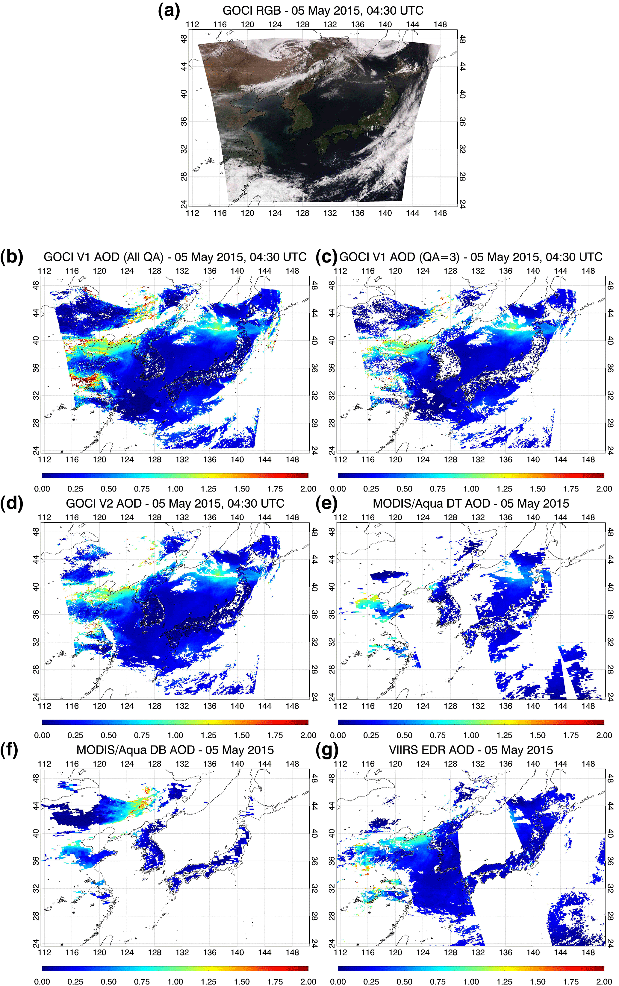
Figure 2(a) GOCI RGB images and AOD for (b) GOCI V1 all QA, (c) GOCI V1 QA3, (d) GOCI V2, (e) MODIS/Aqua DT, (f) MODIS/Aqua DB, and (g) VIIRS EDR algorithms on 5 May 2015 over Northeast Asia.
2.6 Comparison of GOCI YAER V2 AOD with other data
To evaluate the new masking techniques and climatological data used in the V2 algorithm, a retrieved dataset of GOCI YAER V2 AOD for 5 May 2015 is compared with that of the V1 algorithm under two scenarios: using all the quality assured (all QA; QA = 0, 1, 2, or 3) pixels and using only the highest quality assured (QA = 3) pixels. The V2 products are also compared with MODIS/Aqua DT and DB, and VIIRS EDR products (Fig. 2). The overpass times of MODIS and VIIRS are generally near 04:00 UTC over the Korean Peninsula, and thus GOCI 04:30 UTC results are selected for the comparison.
Most land pixels over the Korean Peninsula and Japan are not filtered out and are retrieved as low AOD in the DT, DB, and EDR algorithms. The DB algorithm retrieves high AOD over the bright surface of Manchuria located near 44∘ N, 126∘ E, but the DT and EDR do not retrieve AOD for those pixels because the algorithms are optimized for dark surface reflectance. The DT, DB, and EDR AOD are 0.7–1.2 for land pixels over Hebei in China, located near 38∘ N, 117∘ E. Bright sun glint results in the masking of ocean pixels over the Yellow Sea and East Sea for MODIS and VIIRS, respectively. The EDR algorithm captures an aerosol plume, resulting in AODs of ∼ 0.8 over the northern Yellow Sea, which is not captured by the DT algorithm, and the DT algorithm captures an aerosol plume resulting in AODs of ∼ 0.6 over the East Sea close to Hokkaido, Japan, which is missed by the EDR algorithm.
The all QA GOCI V1 predicts low AOD in Korean Peninsula and Japan areas, but cloud contamination results in high and inhomogeneous AOD, especially near the edge of the cloud cover. Sun-glint-masked ocean pixels are located at lower latitudes for GOCI than for MODIS and VIIRS. Thus, aerosol plumes detected by MODIS and VIIRS are both detected by GOCI. Although the GOCI YAER algorithm targets dark land surface reflectance pixels, as do MODIS DT and VIIRS EDR, the aerosol plume over bright land surfaces in Manchuria captured by the DB algorithm is also detected. However, whether these pixels are from cloud contamination, bright land surface reflectance, or high AOD cannot be determined.
When only pixels with QA = 3 are applied to the V1 algorithm, most high- and inhomogeneous-AOD pixels, typically caused by unfiltered cloud contamination, are removed, but low-AOD pixels over land in South Korea and Japan are also removed. There are two possible reasons for the extensive masking in V1 using only QA = 3 pixels for the case of low AOD over land. The spatial inhomogeneity test of the V1 algorithm is a simple SD of 3 pixel × 3 pixel TOA reflectance with one fixed threshold, regardless of TOA reflectance. Although this approach works well in high-AOD cases, in low-AOD cases, inhomogeneous surface reflectance signals contribute to high SD and result in excessive masking. Another possible explanation is that these pixels have an AOD below −0.05 because of an overestimation of surface reflectance.
Compared with the V1 algorithm, the spatial variability tests of the V2 cloud-masking algorithm consist of the same simple SD test (except for a relaxed threshold), an additional mean-weighted SD test, and a ratio test of the brightest and darkest pixels, relative to TOA reflectance. In addition, darker land surface reflectance is obtained from the climatological data, and this results in increased AOD compared with the large negative AODs seen from the V1 algorithm. Thus, fewer pixels are filtered out using the GOCI V2 algorithm and are retrieved as positive low AOD. The V2 AOD also shows fewer inhomogeneous features near the edges of clouds, similar to the MODIS and VIIRS AOD.
3.1 Ground-based measurements and ancillary satellite data
Two ground-based observation networks – the Aerosol Robotic Network (AERONET) and the Sun-Sky Radiometer Observation Network (SONET) – are used to quantify the accuracy of GOCI YAER V2 AOD (τG−V2) using data from March 2011 to February 2016. AERONET is a ground-based aerosol remote sensing network of CIMEL sun-sky radiometer photometers maintained by the NASA Goddard Space Flight Center (Holben et al., 1998). Spectral AOD and AE are retrieved from direct solar irradiance measurements, and other optical/microphysical properties such as the volume size distribution and refractive indices are retrieved from the inversion of spectral AOD with diffuse-sky radiance measurements. Uncertainties in AERONET AOD (τA) in the visible and NIR have been reported as ±0.01 (Eck et al., 1999), which is much lower than is typical for satellite-retrieved AOD because of the minimal surface-reflectance effects in direct solar irradiance measurements and the highly accurate calibration. Thus, AERONET AOD is often used as the reference dataset for satellite AOD validation. The fully calibrated and cloud-screened AERONET Version 2 Level 2.0 AOD at 550 nm and AE between 440 and 870 nm from direct measurements are used in this study (Smirnov et al., 2000). A total of 27 AERONET sites within the GOCI observation domain, excluding specific short-period campaign sites, are selected for this analysis. Also, AERONET Version 2 Level 2.0 FMF at 550 nm and SSA at 440 nm from inversion products are used for the validation of GOCI FMF and SSA (Dubovik and King, 2000), The SONET is a ground-based aerosol remote sensing network of CIMEL sun-sky radiometers maintained by the Institute of Remote Sensing and Digital Earth, Chinese Academy of Sciences (Li et al., 2015). The SONET also provides spectral AOD (τSONET) from direct sun measurements and AE. A total of six SONET sites in China are selected for the validation of AOD at 550 nm.
In addition, the GOCI V1 AODs with all QA pixels (τG−V1allQA) and only pixels with QA = 3 (τG−V1QA3) are compared with V2 AODs to quantify improvements in the V2 algorithm. The MODIS DT AOD (τMDT) and DB AODs (τMDB) of the highest quality pixels (QA = 3) are also compared over the same site and during the same period to verify the GOCI AOD accuracy. Note that the VIIRS EDR AOD is used in the qualitative comparison in the previous section but is not included in the present validation because the VIIRS data are only available from January 2013.
3.2 Collocation criteria between ground- and satellite-based measurements
The comparison between satellite- and ground-based data is implemented with spatial and temporal collocation criteria. Hourly GOCI AOD pixels that are located within a 25 km radius of each ground site, and ground-based observation data within 30 min of each GOCI observation time, are averaged. The averages from both datasets are included if at least one measurement from each dataset is available. The collocation criteria used for the MODIS data are the same as for GOCI. After the collocation, 27 AERONET sites and 6 SONET sites are matched with GOCI land AOD observations, and 17 AERONET sites are matched with GOCI ocean AOD observations. Note that the 27 AERONET sites matched with GOCI land AOD observations includes all 17 coastal AERONET sites matched with GOCI ocean AOD observations because the coastal sites can be collocated with both land and ocean AOD measurements.
3.3 Statistical evaluation metrics
Following the method of Sayer et al. (2014), the statistical metrics for the evaluation contain the number of collocation data (N); the Pearson's linear correlation coefficient (R); the median bias (MB); the root mean square error (RMSE); and f, the fraction of data points within the expected error range of the MODIS DT AOD (Collection 5), , as described by Levy et al. (2007). Each AOD product has an expected error range that can vary with the algorithm performance. To compare accuracies, the EEMDT is applied to all algorithms. Note that the expected error range of the GOCI YAER V2 AOD (EEG_V2) is estimated independently in Sect. 4.2.
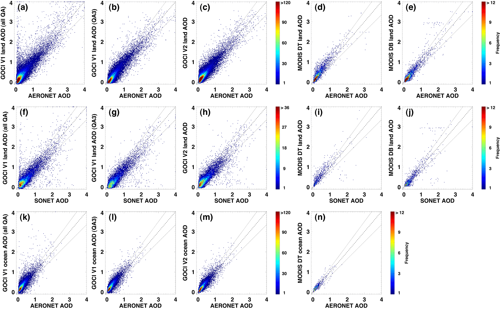
Figure 3Comparison of AOD between AERONET/SONET and GOCI/MODIS DT/MODIS DB over land and ocean surfaces. The x axis is land AERONET AOD, land SONET AOD, and ocean AERONET AOD from top to bottom, and the y axis is GOCI YAER V1 for all QA, GOCI YAER V1 for QA = 3, GOCI YAER V2, MODIS DT, and MODIS DB from left to right. Colored pixels represent a bin size of 0.02. Black dashed lines denote the one-to-one line, and dotted lines denote the expected error range of MODIS DT AOD.
Table 2Statistics of land and ocean AOD comparisons between AERONET/SONET and satellite products, as shown in Fig. 3.
3.4 Validation of GOCI YAER V2 land AOD and comparison with other data
Results of a comparison between AERONET/SONET AOD and GOCI-retrieved AOD over land and ocean surfaces are presented in Fig. 3. Statistics from the comparison are summarized in Table 2. As seen in the qualitative comparison results (Fig. 2), τG_V1allQA shows many overestimated points compared with τA because of remaining cloud contamination. About 20 % of pixels are filtered out with the QA = 3 criteria (τG_V1QA3), and this results in a reduction of the number of overestimated points, decreasing RMSE from 0.24 to 0.18, and increasing R from 0.86 to 0.92. However, underestimated points due to the overestimation of surface reflectance remain, which results in an increase of the negative median bias from −0.015 to −0.066. Results of a comparison of τG_V2 with τA show fewer overestimated points compared with those of τG_V1allQA because of the improved pixel masking. This results in an increased N and f within EEMDT and decreased MB and RMSE compared with τG_V1QA3. The increased N comes from the low-AOD points that are filtered out in τG_V1QA3. The number of underestimated points in the low-AOD range decreased because of decreased surface reflectance using the 5-year samples. This results in lower bias (MB = 0.010), decreased RMSE (0.16), and increased f within EEMDT (0.60). The R of 0.91 is similar to that of τG_V1QA3 (0.92). The N between τA and τG_V2 is about 14 times greater than the corresponding τMDT and τMDB, mostly because of the hourly data available from GOCI compared with the twice-daily overpass data from MODIS. The spread of data points from MODIS and AERONET relative to the one-to-one line is lower than that from GOCI and AERONET, and this results in higher f within EEMDT( 0.62 for τMDT and 0.73 for τMDB). The R and RMSE of τMDT and τMDB are similar to those of τG_V2. The MB of τMDB is closest to zero, and τMDT has a positive MB of 0.043. The overestimation of τMDT has been attributed to the urbanization effect of the biased reflectance estimation (Munchak et al., 2013) and has been corrected in the MODIS DT research algorithm (not used here) using the modified urban surface-reflectance algorithm (Gupta et al., 2016).
The GOCI V2 land AOD results can be recategorized as coastal or inland according to whether each site is collocated with both GOCI ocean and land AOD or with GOCI land AOD only. Mean AERONET AODs from coastal sites are lower (0.28) than those from inland sites (0.42). The intercomparison between coastal-site AERONET AOD and GOCI V2 land AOD has an R of 0.83, RMSE of 0.144, MB of −0.004, and f within EEMDT of 0.60. Results from inland sites have higher R (0.93), RMSE (0.171), MB (0.023), and the same f within EEMDT (0.60). High AOD is detected more frequently at inland sites than at coastal sites.
A comparison between SONET AOD and satellite-retrieved AOD over land reveals that τG_V2 has higher accuracy than τG_V1QA3, except in terms of R. The reason for the decreased accuracy in R of τG_V2 may be the use of the same climatological surface reflectance for each year, whereas in reality the surface reflectance changes annually. The τMDB has the lowest MB and RMSE and highest f within EEMDT. The τMDT has a positive MB of 0.104.
In conclusion, most statistical parameters indicate that land τG_V2 accuracy is improved relative to τG_V1QA3 and is comparable to τMDT and τMDB.
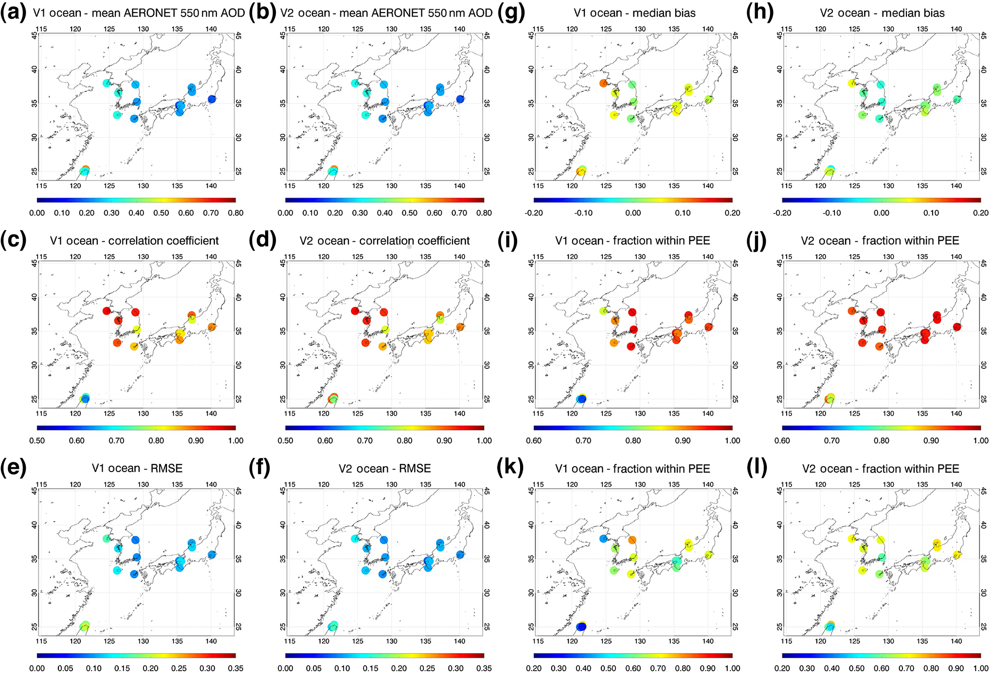
3.5 Validation of GOCI YAER V2 ocean AOD and comparison with other data
The changes of the GOCI YAER algorithm over ocean surfaces between V1 and V2 include the cloud-masking techniques, the use of climatological wind speed data instead of each date data, pixel classification thresholds, criteria for turbid-water and dark-ocean algorithm selection, and the choice of spectral channels. Results from the comparison of τG_V1QA3 with τG_V1allQA show decreased N and RMSE, an MB closer to zero, and increased R and f within EEMDT, which is similar to the results over land sites except for MB. The refinement of the ocean algorithm from V1 to V2 results in improvement in most statistical parameters: decreased MB from 0.043 to 0.008, increased f within EEMDT from 0.62 to 0.71, and decreased RMSE from 0.13 to 0.11. An MB closer to zero means that the modified channel selection in the turbid-water and dark-ocean algorithms, to avoid the effect of water-leaving radiance variation, works effectively. The N between AERONET and GOCI V2 AOD over ocean surfaces is about 27 times greater than that for MODIS DT AOD, which is greater than that seen in the land comparison despite the same difference in observation frequency. The reason for this result is that most turbid-water pixels near the coast are filtered out in the MODIS DT algorithm, but are included in the GOCI YAER algorithm. Compared with the ocean τMDT, the ocean τG_V2 has slightly higher RMSE, an MB closer to zero, slightly higher R, and slightly lower f within EEMDT. In conclusion, most statistical parameters show that ocean τG_V2 accuracy is improved relative to τG_V1QA3 and is comparable with τMDT.
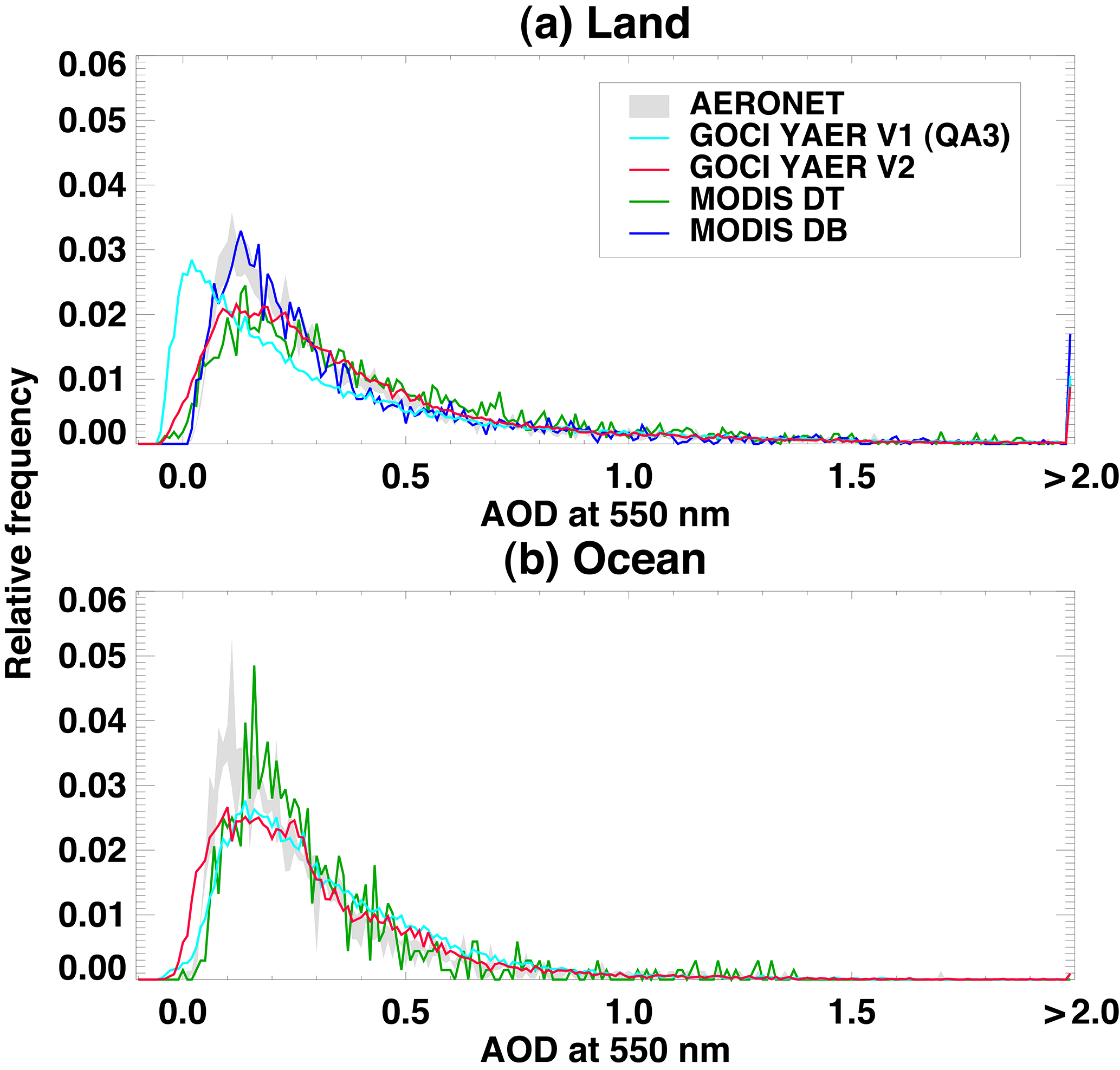
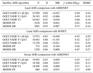
Figure 4Relative frequency histograms of retrieved AOD from AERONET and satellites over (a) land and (b) ocean surfaces.
3.6 Comparison of AOD histogram distribution
In Fig. 4, mean relative frequency histograms for land τA, collocated with GOCI and MODIS land AOD, have a mode of 0.11 (i.e., highest frequency in the range 0.105–0.115) and right-skewed distribution. This is similar to the global τMDT and τMDB mode of 0.1 reported by Sayer et al. (2013). The land τG_V1QA3 mode is 0.02 and those of τG_V2, τMDT, and τMDB are 0.12, 0.10, and 0.13, respectively, which are similar to that of τA. Improvement in the land surface reflectance in V2 results in a reduced difference in mode between AERONET and GOCI. The shape of the histogram of τMDB is better matched to that of τA in the AOD range 0.05–0.30 than to τMDT and τG_V2. The land-targeted histograms of τMDT and τG_V2 have a similar shape to each other. The two histograms have lower frequency modes and higher frequency AOD between 0.3 and 0.7 compared with τA. The τG_V2 has a smoother shape due to a larger number of coincident data points.
The mean relative frequency histograms for τA, collocated with GOCI and MODIS ocean AODs, have a mode of 0.11, and those of ocean τG_V1QA3 and τMDT have modes of 0.14 and 0.16, respectively. However, ocean τG_V2 has a mode of 0.10, which is closer to that of τA than those of τG_V1QA3 and τMDT. Although the mode of ocean τMDT is higher than that of τA, the magnitude of the peak is similar. The histogram distributions of ocean τG_V1QA3 and τG_V2 have lower magnitude peaks and more gradual decreases with increasing AOD compared to τA.
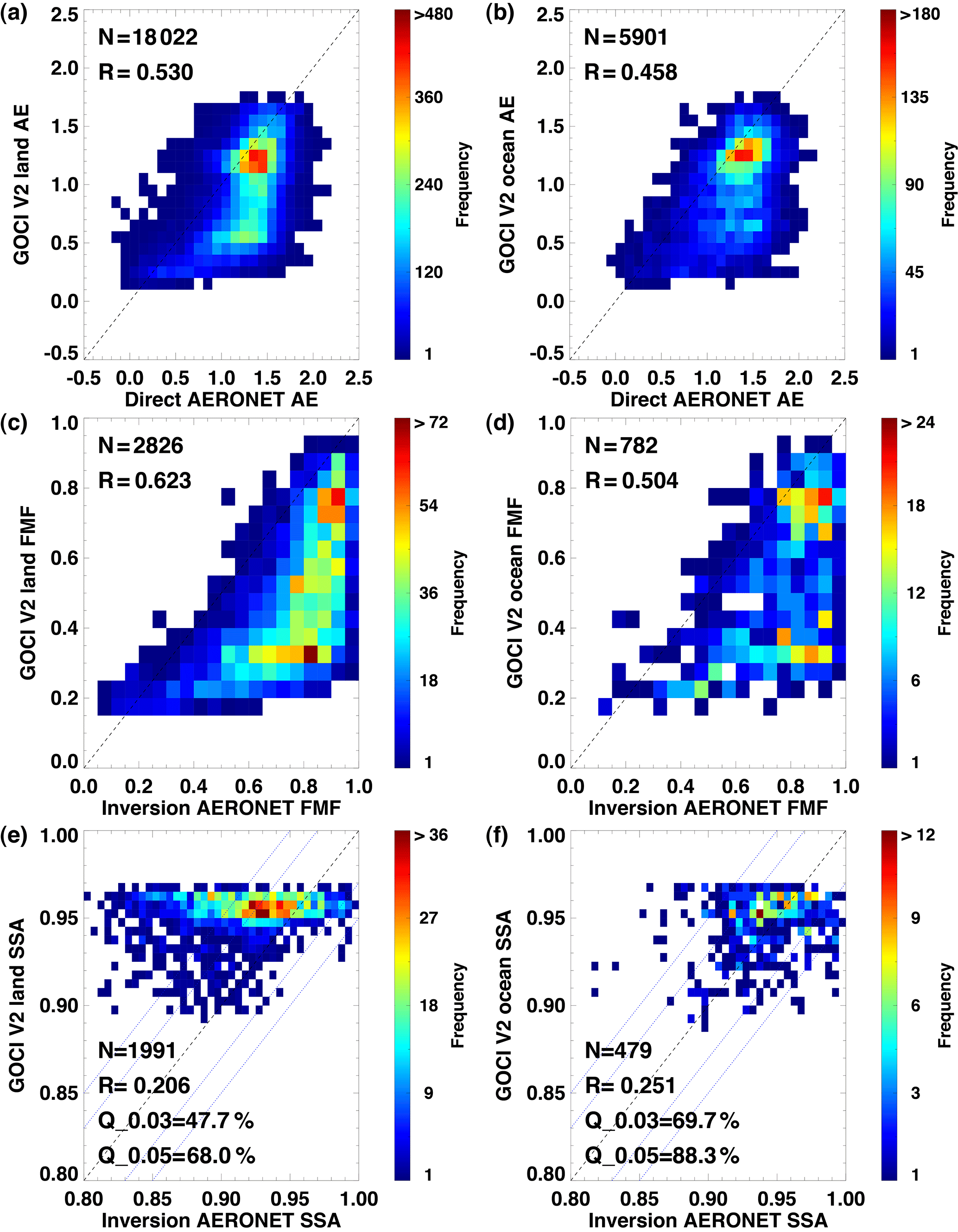
Figure 5Comparison between AERONET and GOCI YAER V2 (a) land AE, (b) ocean AE, (c) land FMF, (d) ocean FMF, (e) land SSA, and (f) ocean SSA. Note that collocated data are only for AERONET AOD > 0.3 for the AE and FMF comparisons, and AERONET AOD > 0.4 for the SSA comparison. Each colored pixel represents a bin size of 0.10 for AE, 0.05 for FMF, and 0.005 for SSA. Black dashed lines denote the one-to-one line, and blue dotted lines in the SSA comparison denote the ±0.03 and ±0.05 ranges.
3.7 Validation of GOCI YAER V2 AE, FMF, and SSA over ocean and land surfaces
The AE intercomparisons between AERONET and GOCI YAER V2 over ocean and land surfaces are presented in Fig. 5a and b. Only AERONET AOD > 0.3 values are included because large errors exist in AE, due to surface reflectance errors when AOD is low. Note that the GOCI AE is derived from the predefined values of the selected aerosol model, not from the retrieved spectral AOD. Compared with the V1 AE accuracy during the DRAGON-NE Asia 2012 campaign described by Choi et al. (2016; R= 0.678 over both land and ocean surfaces), the V2 land and ocean AE have lower linear correlations with AERONET (R= 0.505 and 0.459, respectively) from the 5-year validation. The DRAGON-NE Asia 2012 campaign was conducted in spring (March–May) when long-range transport of yellow dust from the Gobi and Taklamakan deserts in Asia, which has low AE with high AOD, is more frequent. Aerosol plumes with low AE and high AOD can be retrieved with higher accuracy compared with the generally low-AOD cases during other seasons. Thus, AE shows stronger linear correlation in spring (R of 0.63 over land and 0.57 over ocean) but is lower for other seasons (R of 0.24 over land and 0.22 over ocean). The highest frequency of points is close to the one-to-one line, but there is a significant discrepancy when AERONET AE is ∼ 1.3 but GOCI AE is ∼ 0.6, particularly over land. This could be caused by varying surface reflectance errors for each channel or perhaps by a local-minimum problem induced from the LUT approach used for inverse modeling.
The FMF intercomparisons between AERONET inversion data and GOCI YAER V2 are similar to those of AE, as shown in Fig. 5c and d. This comparison also includes only AERONET AOD > 0.3 data. AERONET inversion products are retrieved from almucantar measurements, which are possible when the solar zenith angle is greater than 50∘ (Dubovik and King, 2000); thus, the number of points used in the comparison are fewer than the AOD and AE from direct measurements. The correlation coefficients of FMF over ocean and land surfaces are similar to those of AE, as both parameters are determined primarily by aerosol size.
The SSA intercomparisons between AERONET and GOCI YAER V2 have the lowest R (0.206 for land and 0.251 for ocean) among the products. The visible–NIR wavelength range is more sensitive to aerosol size than absorptivity. Thus, aerosol models are constructed more coarsely for SSA than for FMF, and the inversion methods focus on spectral matching of AOD at 550 nm, rather than on SSA-optimized retrieval, such as the OMI aerosol retrieval algorithm using ultraviolet radiation (Torres et al., 2013; Jeong et al., 2016). Nevertheless, the ratio of GOCI V2 SSA to AERONET SSA in a ±0.03 and ±0.05 range is 47.7 and 68.0 % for land and 69.7 and 88.3 % for ocean, respectively, which is comparable to the OMI SSA presented by Jethva et al. (2014).
In conclusion, GOCI YAER V2 AE, FMF, and SSA compared with AERONET products are more biased and have lower correlation coefficients than seen for AOD. This indicates that the aerosol type selection is biased to coarse and nonabsorbing aerosols. To improve the accuracy of these parameters, more accurate surface reflectance estimations and improved inversion methods are required.
Retrieved AOD likely has both a systematic and random error associated with various factors, including sun–earth–satellite geometry, cloud contamination, surface type, and assumed aerosol model, among others. An error analysis of satellite AOD can help identify the most important contributors to errors in these products. In this section, coincident GOCI and AERONET AOD are analyzed to quantify systematic and random errors. A systematic bias analysis is implemented for the four GOCI products (i.e., the V1 land AOD with QA = 3, V2 land AOD, V1 ocean AOD with QA = 3, and V2 ocean AOD). In addition, pixel-level uncertainties in GOCI version 2 land and ocean AOD are estimated.
4.1 Systematic bias analysis
4.1.1 Bias as a function of AERONET AOD
As shown in Fig. 6a, V1 land AOD has a negative bias in the low-AOD range because of an overestimation of surface reflectance. After implementing climatological surface reflectance over land, the V2 land-AOD shows less bias than that of V1 and is close to 0 over the whole AOD range. This results from the increased probability of finding observation days with low aerosol loading using a 5-year dataset. The V2 ocean AOD shows a positive bias around 0.05–0.10 and high positive bias of 0.1 when AERONET AOD is ∼ 0.3. The reason for the positive bias in ocean AOD may be an underestimation of ocean surface reflectance when considering only climatologically averaged wind speed and geometry, without accounting for changes in surface properties including bio-optical properties. Details of improvements to the ocean AOD calculation are described later. The ranges of the 16th–84th percentiles of both land and ocean AOD become wider as AERONET AOD increases, and the shapes of the ranges are asymmetrical.
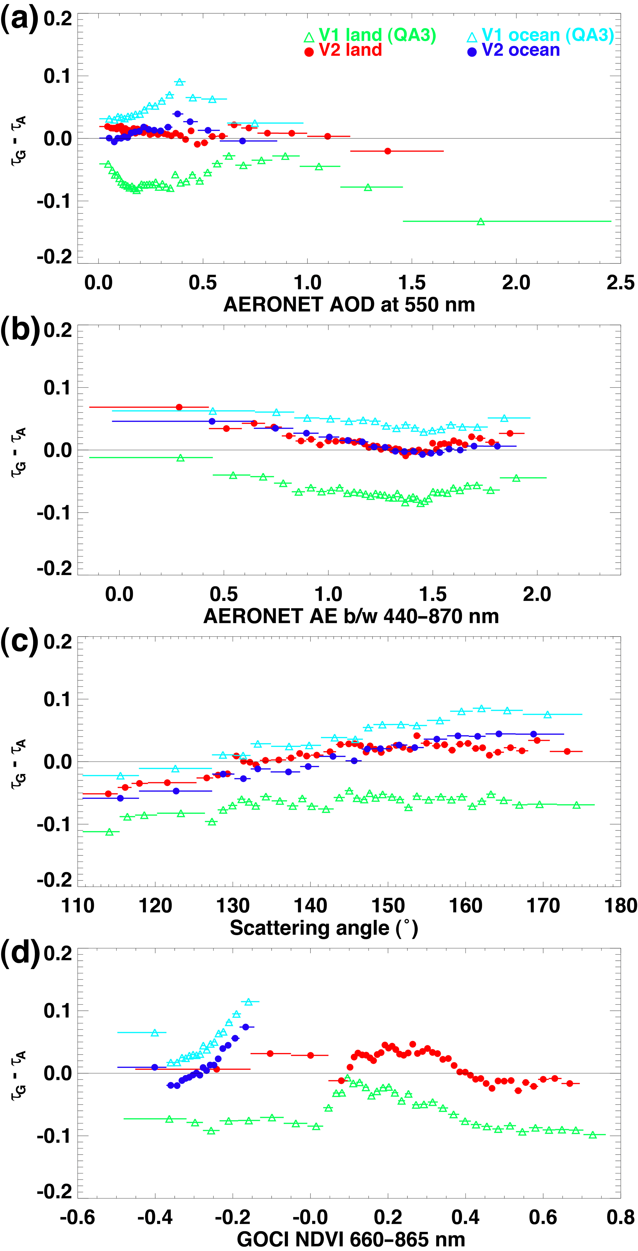
Figure 6Difference between GOCI and AERONET AOD in terms of (a) AERONET AOD, (b) AERONET AE, (c) scattering angle, and (d) GOCI NDVI. Each point represents the 50th percentile of 1000 collocated data points sorted in ascending order for each x axis value. The horizontal line through each point represents the range of collocated data points.
4.1.2 Bias as a function of AERONET AE
The V2 ocean and land AOD biases are close to zero when AERONET AE is within 1.3–1.6 and the accuracy of GOCI AE is high (Fig. 6b). However, these biases increase in the positive direction as AE deceases to 0.3 (large particles). Compared with the biases of V1, those of V2 are reduced for all AE ranges, but the pattern of difference in AE remains. This could be due to errors in the assumed aerosol optical properties of extremely large particles. Assumed aerosol models based on the global AERONET climatological database are categorized according to FMF and SSA, and the phase functions of nonspherical properties are averaged to one value for each model. In reality, various nonspherical shapes with the same FMF value may be present and may result in higher error at low values of AERONET AE. The differences may also be due to errors in aerosol type selection during the inversion process, as suggested by the decreased accuracy of low GOCI AE. Wavelength-dependent errors in calibration or surface reflectance assumptions may also contribute to the observed differences. Further investigation is required to quantify the relative contributions of these errors.
4.1.3 Bias as a function of scattering angle
In Fig. 6c, the bias of ocean AOD changes from −0.05 to 0.10 as scattering angle increases from 110 to 175∘. The bias in land AOD shows a similar trend, but with a range of variance from −0.05 to 0.05. As the scattering angle increases to 180∘, the atmospheric contribution to total TOA reflectance decreases compared with that from the surface because of the shorter light path length, which leads to an increase in AOD retrieval error (Sayer et al., 2013). This larger error at higher scattering angle is more distinct for ocean AOD than land AOD because of the difference in surface reflectance. The land algorithm performs characterization at each hour for surface reflectance using the composite method to reflect the BRDF effect. The ocean algorithm also considers geometry and wind speed in calculating the BRDF effect. However, ocean bio-optical properties such as chlorophyll (Chl) or color-dissolved organic matter (CDOM) are not considered in the current ocean surface reflectance calculation. This may be the cause of the relatively large error in ocean AOD compared with land AOD.
4.1.4 Bias as a function of NDVI
A bias analysis of land and ocean AOD relative to NDVI is presented in Fig. 6d. The V2 land AOD has a bias close to zero for NDVI > 0.4 (high vegetation), but has a positive bias of up to 0.05 in the range 0.1 < NDVI < 0.4, which corresponds to less vegetated areas, such as semiarid and urban regions. The method used to determine surface reflectance from multi-year samples in the V2 algorithm is applied to all pixels identically regardless of surface type, which can result in a bias that varies with NDVI. The positive bias over urban areas is similar to that of the MODIS Collection 6 DT AOD (Munchak et al., 2013; Gupta et al., 2016). The positive bias of V1 ocean AOD is generally lower using the V2 algorithm because the 500–600 nm channels that are strongly affected by ocean bio-optical property variance are not used in the V2 ocean algorithm. However, channels that are used in the V2 algorithm can still be slightly affected by these bio-optical effects. Thus, positive biases persist for smaller negative NDVI values, which correspond to less turbid ocean pixels where ocean surface models that consider wind speed are utilized.
4.1.5 Bias as a function of cloud contamination
Despite applying several cloud-masking techniques, the remaining cloud-contaminated pixels may still result in high positive biases in AOD. In this section, uncertainties due to cloud contamination are analyzed in terms of (1) cloud fraction at the aerosol product pixel resolution (6 km × 6 km), (2) the number of GOCI aerosol pixels collocated with each AERONET site, and (3) AOD spatial homogeneity.
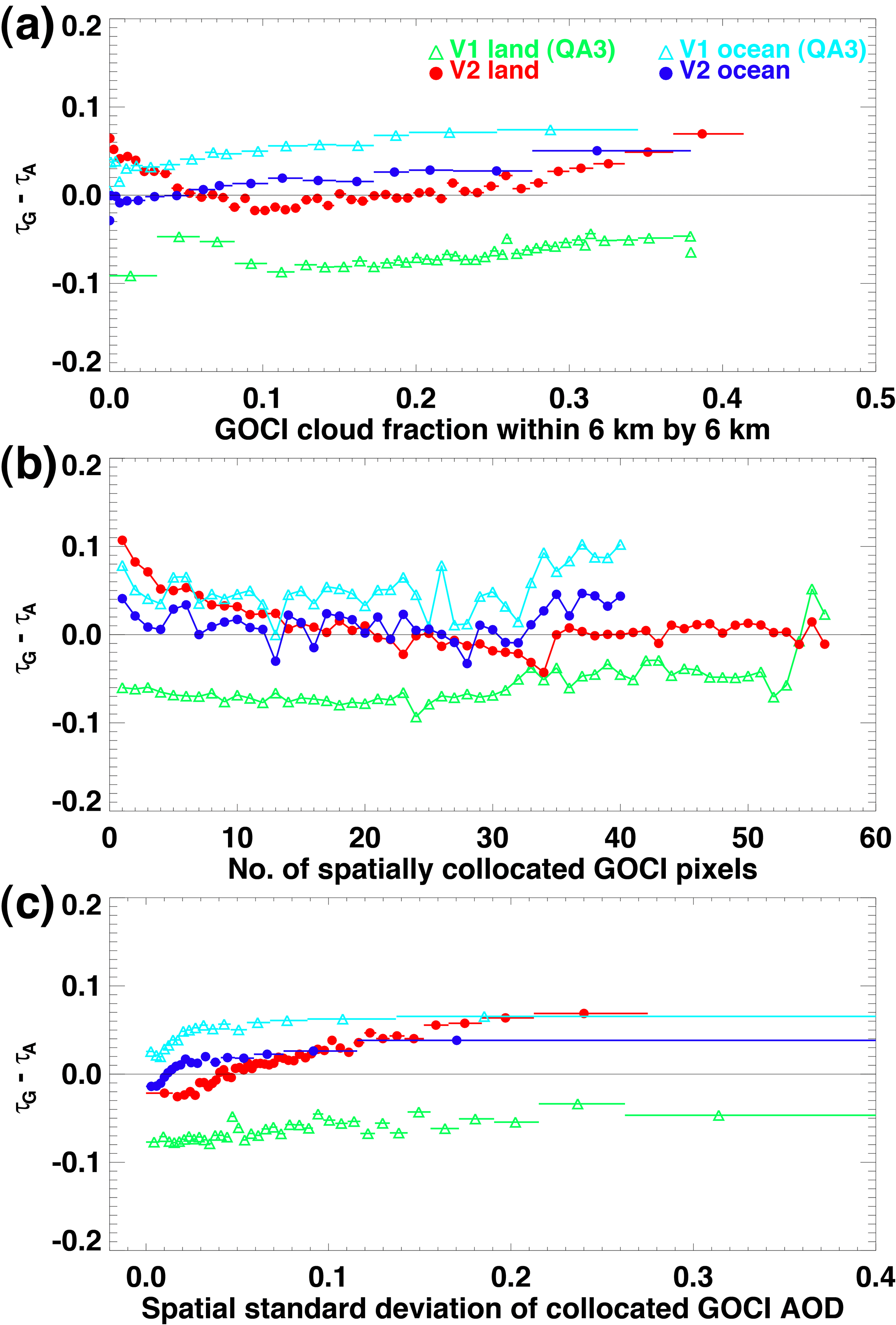
Figure 7Difference between GOCI and AERONET AOD in terms of (a) GOCI cloud fraction within each aerosol product pixel (6 km × 6 km), (b) the number of spatially collocated GOCI pixels within a 25 km distance from AERONET sites, and (c) the spatial standard deviation of collocated GOCI AOD. The points, dotted lines, and horizontal lines in (a, c) are as defined in Fig. 6.
First, the cloud fraction (CF) for one 6 km × 6 km aerosol-product pixel can be calculated using the number of 0.5 km × 0.5 km L1B pixels that remain after all masking steps. In the aggregation step from the original L1B resolution of 0.5 km × 0.5 km to Level 2 aerosol-product resolution of 6 km × 6 km, the maximum number of remaining pixels is 58 after performing all the individual masking processes and discarding the darkest 20 % and brightest 40 % of pixels in a block of 12 pixels × 12 pixels (i.e., 144 pixels). The minimum number is set as 29, which corresponds to 50 % of the maximum value. If the number of remaining pixels is less than 29, then AOPs of that pixel are not retrieved. Note that pixels that are bright because of surface reflectance, not clouds, may be counted as a high CF, but it is difficult to completely distinguish these two cases at 500 m spatial resolution. In Fig. 7a, the bias of ocean AOD is close to zero for a CF of 0.0, and increases to 0.1 as the CF increases to 0.5. The bias of land AOD is ∼ 0.05 when the CF is close to zero, approaches to zero for 0.05 < CF < 0.25, and increases up to 0.05 as the CF goes to 0.4. This positive bias under high-CF conditions is similar to that of MODIS DT and DB AOD (Hyer et al., 2011; Shi et al., 2013). However, the positive bias of land AOD at CF = 0, which is not observed for MODIS DT and DB AOD, may be due to surface reflectance underestimations over bright surface in GOCI.
Next, the bias due to cloud contamination is analyzed with reference to the number of spatially collocated GOCI AOD pixels of each scene (NC) for each AERONET site location (Fig. 7b). Because the GOCI AODs within a 25 km radius around each site are averaged if at least one pixel is available, NC can indicate the existence of clouds near the AERONET site over a broader domain. Note that the maximum NC of ocean AOD pixels of 40 is less than that of land (56) because ocean AOD is generally collocated with AERONET sites located on the coast. The bias of V2 land AOD is 0.1 for NC= 1 and approaches zero as NC increases. The V1 land AOD had a negative bias, primarily because of surface reflectance. Thus, the bias does not change with NC. The ocean AOD bias is 0.05 for NC= 1 and decreases for higher NC, up to 30. However, high positive biases exist for NC > 30, which could be due to problems in characterizing ocean surface reflectance.
Finally, the SD of the spatially collocated AODs indicates how spatially smooth the retrieved AODs are. In the GOCI algorithm, aerosol optical properties for each pixel are retrieved independently regardless of the surrounding pixels, which is similar to the approach used by the MODIS DT and DB algorithms (Hsu et al., 2013; Levy et al., 2013). The SD could increase if cloud-contaminated pixels are misclassified as high-AOD pixels, despite the presence of relatively low AOD in the surrounding pixels. Thus, the SD may be an indirect indicator of cloud contamination in this independent-pixel retrieval method. In Fig. 7c, the bias increases positively up to ∼ 0.13 for ocean AOD and to ∼ 0.08 for land AOD as the SD increases. The 16th–84th percentile range also becomes wider (not shown). The V1 land AOD had negative biases of −0.1 for low SD and −0.05 for high SD and was persistently affected by surface reflectance issues and/or cloud contamination. Note that some recent aerosol retrieval algorithms have adopted a statistical spatial smoothness constraint for AOPs in the inversion procedure to improve accuracy (Dubovik et al., 2011; Xu et al., 2016).
In summary, the high cloud contamination in both each product-pixel (6 km × 6 km) and neighboring pixel (within 25 km) domains results in high positive biases of up to 0.1. However, an independent analysis of the cloud-contamination-only effect is complicated by various factors including surface reflectance errors, resulting in a high bias under low cloud-contamination conditions.
4.1.6 Bias as a function of hour, month, and year
The GOCI AOD consists of eight hourly observations per day from 09:30 to 16:30 KST (centered time of each measurement), and the solar zenith and azimuth angle varies over a much wider range than that of low earth orbit (LEO) satellites. However, it requires more sophisticated treatments for properties such as surface reflectance, the aerosol phase function, and the calculation of Rayleigh scattering, which may result in accuracies that vary with measurement time. In Fig. 8a, the bias of land AOD decreases from about −0.1 for V1 to almost zero for V2, with no noticeable hourly dependence for V2. In contrast, the ocean AOD has a distinct diurnal bias shape, which is close to zero at 09:30, 15:30, and 16:30 KST and ∼ 0.1 at 12:30 KST. This is consistent with the results of the bias analysis with reference to the scattering angle.
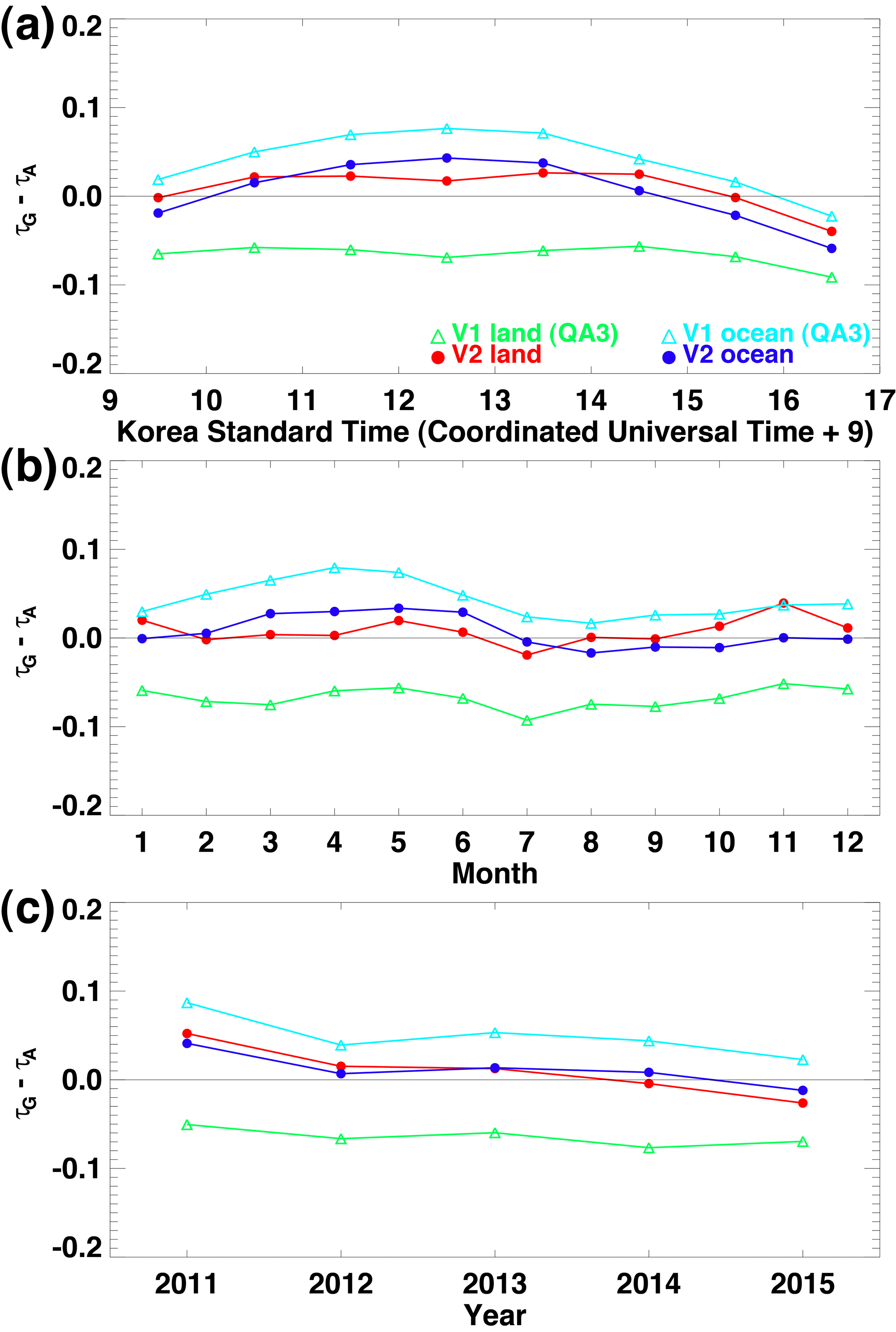
Figure 8Difference between GOCI and AERONET AOD in terms of local observation time, month, and year. The points are as defined in Fig. 7b.
The bias of land AOD as a function of month remains near zero (Fig. 8b). In contrast, that of ocean AOD increases up to 0.1 in spring (April–May) and to ∼ 0.05 in late fall and early winter (November–December), which can likely be attributed to monthly variations in Chl concentration over East Asia. The climatological Chl concentration reported by Yamada et al. (2004) is highest during spring (1.2–2.7 µg L−1), lower during late fall (0.8–1.2), and 0.2–0.4 µg L−1 during other seasons. Thus, the change in monthly bias for ocean AOD is likely affected by Chl concentrations in the current GOCI ocean AOD algorithm. The positive biases of the V1 ocean AOD during spring and late fall were reduced using V2 after changing the channel selection.
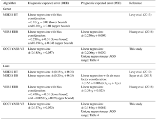
Table 3Expected errors of MODIS C6, VIIRS EDR, and GOCI over ocean and land. μ0 and μ are the cosine of solar zenith angle and satellite zenith angle, respectively. τA and τS are AERONET and satellite AOD, respectively.
The V1 land AOD retrieved using monthly surface reflectance data for each year shows a constant negative bias of about −0.05 from 2011 to 2015 (Fig. 8c). In contrast, the V2 land AOD retrieved using monthly climatological surface reflectance data from the 5-year dataset samples shows biases that are smaller than those of V1 but with increased variation. The increased variance for V2 could be due to a limitation of the application of climatological data, which cannot reflect year-to-year changes in surface reflectance. The ocean AOD shows less variation in bias compared with the V2 land AOD, but it varies more than the V1 land AOD. This may be attributable to interannual variations in ocean surface reflectance caused by ocean bio-optical properties.
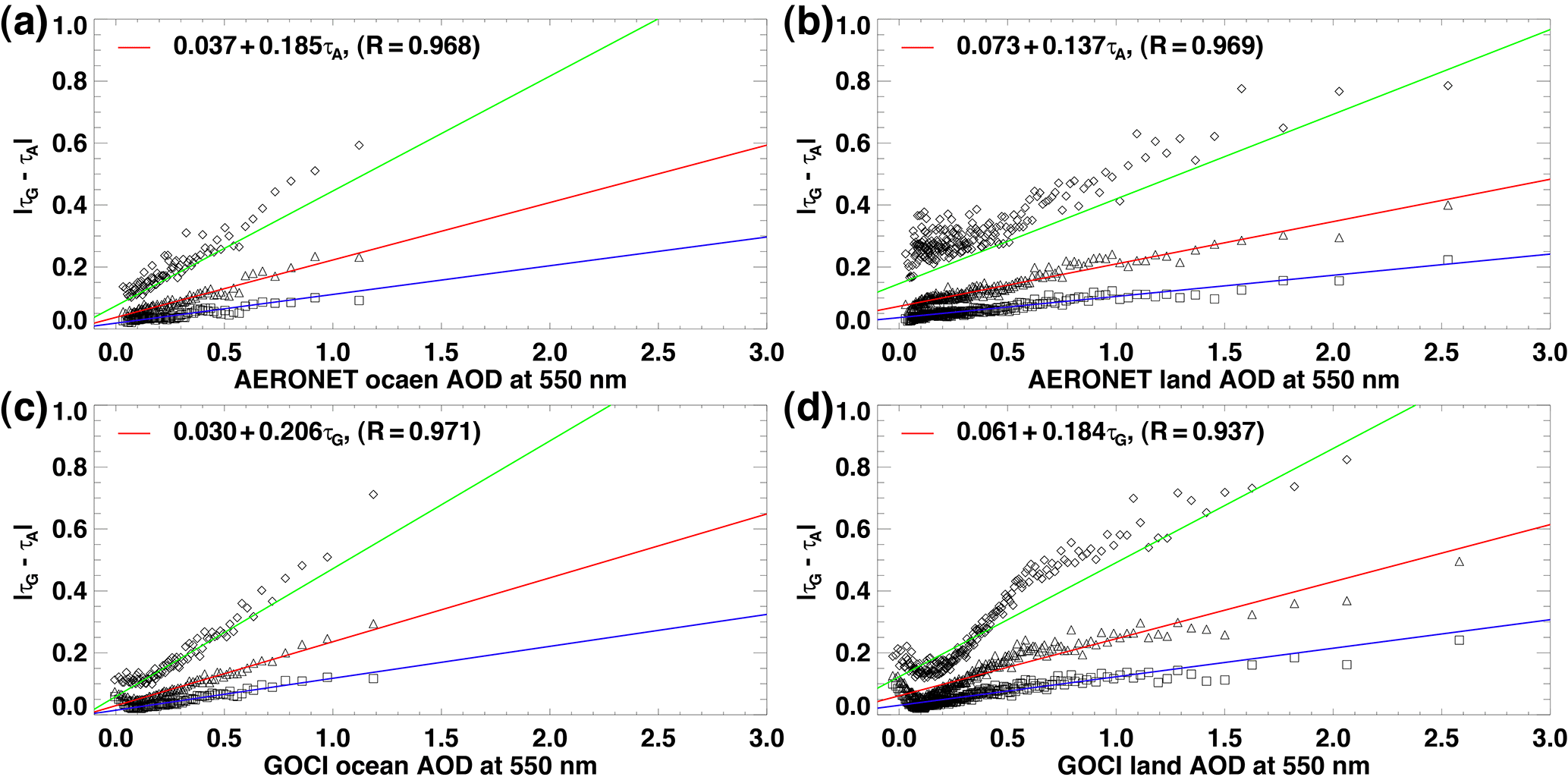
Figure 9Absolute difference between GOCI YAER V2 AOD and AERONET AOD in terms of (a) AERONET ocean AOD, (b) AERONET land AOD, (c) GOCI YAER V2 ocean AOD, and (d) GOCI YAER V2 land AOD. The diamond, triangle, and square symbols represent the 38th, 68th, and 95th percentiles of 200 collocated data points sorted in ascending order of x axis value. In (a–d), the red line in each panel is the linear least-squares fit of the 68th percentiles, and the blue and green lines are half and double the red line values, respectively.
4.2 Uncertainty estimation for GOCI YAER V2 AOD
The uncertainty (or “expected error”) of retrieved AOD is defined as a 1 SD confidence interval corresponding to the 68th percentile, and it is estimated from the long-term evaluation of retrieved satellite AOD using ground-based AERONET measurements. Each satellite-retrieved AOD has its own uncertainty based on the methods used for surface reflectance estimations, assumed aerosol models, etc. The expected error (EE) of retrieved AOD can be estimated as a function of both AERONET AOD and retrieved satellite AOD. The “diagnostic” expected error (DEE) is based on AERONET AOD, which is more accurate than satellite AOD and is thus more useful in quantitatively evaluating the algorithm, though it is restricted to only the AERONET pixels. Alternatively, the “prognostic” expected error (PEE), a function of retrieved satellite AOD, can be calculated over all retrieved pixels, making it more appropriate for certain applications, such as data assimilation with air-quality forecasting models (Sayer et al., 2013; Shi et al., 2013). A common characteristic of EE is that it increases linearly with AOD. Thus, a linear regression fit between the 68th percentile of absolute error and the reference AOD (AERONET or satellite AOD) is determined as EE. The 68th, 38th, and 95th percentile points correspond to 1, 0.5, and 2 SD intervals, respectively, assuming the error has a Gaussian distribution and no bias. Thus, 0.5 and 2 times the linear least square regression equation of the 68th percentile should correspond to the 38th and 95th percentiles, respectively. The EEs of MODIS, VIIRS, and GOCI AOD based on this approach are summarized in Table 3. Note that additional factors are considered in the EE calculations for each algorithm, such as bias information in MODIS DT over ocean surfaces and VIIRS EDR, and geometrical air mass factors in MODIS DB (Levy et al., 2013; Sayer et al., 2013; Huang et al., 2016).
Table 4Prognostic expected error (PEE) estimation of GOCI YAER V2 AOD according to the AOD range. The minimum PEE is labeled “noise floor”.
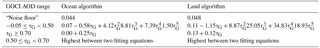
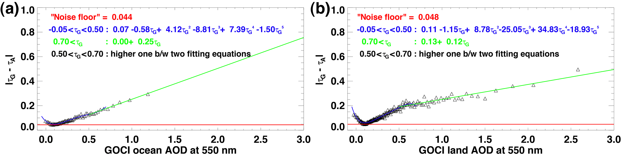
Figure 10Absolute difference between GOCI YAER V2 AOD and AERONET AOD in terms of (a) GOCI YAER V2 ocean AOD and (b) GOCI YAER V2 land AOD. The triangle symbols represent the 68th percentiles of 200 collocated data points sorted in ascending order of x axis value.
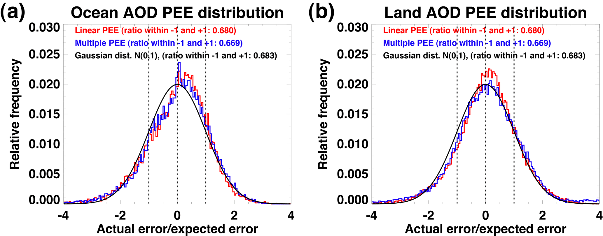
Figure 11Comparison of observed (a) ocean and (b) land AOD error distributions with theoretical Gaussian distributions for the linear PEE (red) and multiple PEE (blue).
Figure 12Spatial distribution of statistical evaluation metrics for GOCI YAER V1 QA3 land AOD (first and third columns) and V2 land AOD (second and fourth columns). Left panels show mean AERONET AOD, correlation coefficient, and RMSE from top to bottom. Right panels show median bias, fraction within DEE, and fraction within multiple PEE from top to bottom.
To estimate DEE and PEE of the GOCI YAER V2 AOD using a linear least-squares regression equation, the absolute AOD difference between GOCI and AERONET is analyzed for AERONET and GOCI AOD in Fig. 9. The linear DEE (0.185τA+0.037) and PEE (0.206τG+0.030) of ocean AOD follow the 68th percentile points well (R= 0.968 and 0.971, respectively). Doubled values of DEE and PEE for ocean AOD are well matched with the 95th percentile points. Although the linear DEE (0.137τA+0.073) and PEE (0.184τG+0.061) of land AOD are well matched with the 68th percentile points (R= 0.969 and 0.937, respectively), the PEE of land AOD includes discrepancies that vary over the AOD range. Significant discrepancies exist between the 95th percentile points and doubled values of the PEE of land AOD. Due to the existence of more complex error sources, the EE of land AOD cannot be accurately characterized in a linear relationship with AOD (Hyer et al., 2011). The estimated linear DEE and PEE of land AOD show similar or lower slopes but higher offset compared with MODIS and VIIRS, which is assumed to be due to higher surface reflectance bias in GOCI.
Instead, PEE values constructed for specific AOD ranges (“multiple PEE”) are applied as in Fig. 10 and summarized in Table 4. The “noise floor”, defined by Hyer et al. (2011), is the minimum absolute error. A fifth-order polynomial regression fit is applied for GOCI AOD < 0.5 to reflect the curved pattern, and a linear fit is applied when GOCI AOD > 0.7. The higher of these two computed values is applied when GOCI AOD is between 0.5 and 0.7. Both multiple PEEs show higher EE values near GOCI AOD of 0.1 (over ocean and land) and 0.6 (over land) compared with the linear PEEs, and thus they better match observations near the 68th percentile.
The ratio of actual error to linear and multiple PEE follows the theoretical Gaussian distribution with a mean of zero and variance of 1 (N(0,1)) as shown in Fig. 11, which is similar to the results obtained for MODIS DB AOD (Sayer et al., 2013). Because the PEE of ocean AOD has a strong linear relation with GOCI AOD, there are fewer differences between linear and multiple PEE. However, the PEE of land AOD has a significantly different relationship with AOD, leading to differences in the distributions of linear and multiple PEE. Although the ratio between 1 and 1 (0.683) is closer to that of linear PEE for land AOD (0.680) than to the corresponding multiple PEE (0.669), the peak of N(0,1) is closer to that of multiple PEE than linear PEE. In addition, all linear and multiple PEEs of ocean and land AOD have slight positive biases compared with N(0,1). Notwithstanding, the obtained PEEs of GOCI YAER V2 AOD, particularly multiple PEE for land AOD, generally represent actual errors well.
4.3 Regional performance
The obtained GOCI DEE and (multiple) PEE can be used for AOD validation for each site along with other statistical evaluation metrics presented earlier. The validation results for all sites have been analyzed individually to compile the results shown for each site, including the fraction of data points within DEE and (multiple) PEE. Spatial distributions of statistical evaluation metrics are presented in Figs. 12 and 13 for land and ocean AOD, respectively.
The average of collocated AERONET AOD is highest in China, including the Beijing (0.69 and 0.48 with GOCI V1 and V2, respectively) and Taihu (0.70) sites. The South Korean sites show higher annual average AERONET AOD (0.33–0.50) than Japanese sites (0.17–0.30). For land AOD among the 27 land AERONET sites, 21 sites show improvement in V2 according to the statistical evaluation metrics and 6 sites have decreased accuracy in V2 compared with V1. In addition, the GOCI V2 land AOD shows less bias and has a higher fraction of data points within DEE and PEE over the Korean Peninsula compared with the Chinese and Japanese sites. The sites with the worst accuracy in V2 land AOD have a positively increased median bias. The reason for this decrease in accuracy of some of the sites in V2 compared with V1 is likely the way that the surface reflectance database is constructed. Surface reflectance at the lower accuracy sites in V2, such as at Chiba University, Kobe, Xinglong, and Osaka, is brighter (urban surfaces) than at other sites, and the current identification threshold of the darkest 1–3 % of observations, without considering surface type, results in climatologically derived values for reflectance that are too dark at bright (urbanized) surface sites. Tilstra et al. (2017) suggested that selecting the mode of the RCR histogram improves the characterization of surface reflectance of bright surfaces compared with selecting the minimum values of the RCR. Choosing different thresholds for various surface types may improve the accuracy of retrievals over sites that have high surface reflectance.
For ocean AOD, 14 sites show improvement in V2 and 3 sites have lower accuracy in V2 than V1 among the 17 coastal AERONET sites. In contrast to the increased median bias in land AOD, ocean AOD shows decreased median bias from V1 to V2. However, the lower accuracy sites do not differ significantly between V1 and V2 compared with land AOD. The fraction of data points within DEE and PEE for V1 ocean AOD at the Japan sites is higher than at the South Korean sites, but becomes similar in V2. The obtained DEE of V2 ocean AOD (94 %) is higher than the theoretical 1σ fraction (68 %). However, the PEE of V2 ocean AOD is 66 %, similar to the theoretical value. Thus, the obtained PEE can represent the error of GOCI AOD better than DEE.
Aerosol retrieval using GOCI is unique because of hourly monitoring of aerosols with multi-channel measurements in the visible to near-infrared range with high spatial resolution, over East Asia where aerosol emissions are very high, despite its limitation in observation area coverage. Hourly GOCI AOD retrievals with high accuracy, NRT availability, and quantitatively analyzed uncertainties are highly suitable for use with air-quality monitoring and data assimilation in air-quality forecasting models, particularly when rapid diurnal variations and transboundary transport are significant.
The objective of this study is the development of an improved GOCI YAER algorithm (V2) for NRT processing with higher accuracy. Cloud-masking procedures were revised to prevent false masking of low-AOD pixels over bright surfaces that was present in the previous version by adopting recent MODIS and VIIRS cloud-masking methodology and improving existing V1 methodologies. To reduce the remaining cloud and aerosol contamination effects in the surface reflectance database, the period of RCR samples is expanded from a 1-year to a 5-year period, to increase the probability of finding cloudless low-AOD cases that improve the accuracy of the climatological surface reflectance database. In addition, the surface wind speed data are constructed as a climatological database for NRT retrieval without importing numerical weather forecast products. The GOCI spectral channel selection is revised to account for specific surface conditions: dark ocean, turbid water, and land surface. In particular, the channels from 500 to 700 nm, which are significantly affected by ocean bio-optical variations, are excluded from ocean AOD retrievals. As a result, the area of successful AOD retrieval and masking in the GOCI YAER V2 algorithm and the retrieved AOD values approach the results of MODIS and VIIRS AOD qualitatively, compared to that of GOCI YAER V1.
To confirm the improvements to GOCI AOD accuracy in V2, the retrieved GOCI AOD and MODIS AOD are compared with ground-based East Asia AERONET and China SONET measurements of AOD for 5 years from 1 March 2011 to 29 February 2016. The GOCI YAER land AOD shows a significant improvement from V1 to V2 with reduced bias from about −0.07 to 0.01 and increased f within EEMDT from 49 to 60 %. The comparison with SONET AOD also shows improved results with reduced bias from about −0.10 to −0.02 and increased f within EEMDT from 42 to 51 %. The GOCI YAER ocean AOD also shows reduced bias from about 0.04 to 0.01 and increased f within EEMDT from 62 to 71 %. As a result, the quality of both the GOCI YAER V2 ocean and land AOD is more comparable to that of the MODIS DT and DB AOD products over East Asia.
Although retrieved GOCI YAER V2 AOD shows some bias with respect to AERONET AOD and AE, scattering angle, NDVI, cloud fraction and homogeneity of retrieved AOD, and observation time, month, and year, it never exceeds an absolute value of ∼ 0.1 for most variables. Accounting for the observed increase in error with AOD, the intrinsic expected error of GOCI YAER V2 AOD was estimated using AERONET data. The linear DEE and PEE (0.185τA+0.037 and 0.206τG+0.030, respectively) for ocean AOD represent the actual error well over the entire AOD range. The linear DEE of land AOD (0.137τA+0.073) also represents the actual error well. However, the actual error does not increase linearly with GOCI land AOD; thus, the linear PEE of land AOD (0.184τG+0.061) shows variations over the AOD. Instead, the use of multiple PEE, which consists of PEE values for specific GOCI AOD ranges, improves the representation of the actual error.
Despite the algorithm improvements presented in this study, there is still potential for future improvements. The current version of the LUT was calculated using a scalar radiative transfer calculation, which is less accurate for calculating Rayleigh scattering for short visible wavelengths (∼ 400 nm), and using a plane-parallel atmosphere approximation that is less accurate at high solar/sensor zenith angle. Vector radiative transfer calculations (i.e., consideration of polarization) and spherical-shell atmosphere approximations can calculate Rayleigh scattering at high accuracy and may improve the accuracy of the GOCI YAER algorithm. Also, recent statistically optimized aerosol retrieval algorithms utilizing the characteristics of spatial and temporal smoothness constraints for aerosols result in improved accuracy by increasing the aerosol signal (Dubovik et al., 2011; Xu et al., 2016). They also enable the simultaneous retrieval of multiple geophysical variables, such as aerosol and surface reflectance over land and aerosol and chlorophyll concentrations over the ocean, which can reduce the remaining error due to the predefined surface reflectance over ocean and land surfaces in the GOCI YAER algorithm.
The second-generation GOCI (GOCI-II), scheduled to launch in 2019, which has higher spatial resolution (∼ 250 m), more channels, including 380 nm, and daily full-disk coverage, will further improve the accuracy of AOP retrieval. Furthermore, GOCI-II will observe East Asia simultaneously with the Geostationary Environmental Monitoring Spectrometer (GEMS) for trace gases (i.e., ozone, nitrogen dioxide, formaldehyde, and sulfur dioxide) and the AMI for meteorological parameters (i.e., cloud properties). Therefore, multi-sensor synergies contributing to a comprehensive understanding of aerosols and trace gases, cloud, and ocean colors are expected.
The GOCI L1B data are available on the home page of the Korean Institute of Ocean Science and Technology (KIOST) Korea Ocean Satellite Center (KOSC, 2018; http://kosc.kiost.ac.kr/), and the GOCI YAER V2 aerosol data will be available at the same site. The GOCI YAER V2 aerosol data are also available through personal communication with the authors of the present paper. The AERONET data were obtained from https://aeronet.gsfc.nasa.gov (GSFC, 2018). The SONET data were obtained from http://www.sonet.ac.cn (SONET, 2018). The MODIS DT and DB aerosol data were obtained from https://ladsweb.modaps.eosdis.nasa.gov (LAADS DAAC, 2018). The VIIRS EDR aerosol data were obtained from https://www.class.ncdc.noaa.gov (NOAA, 2018). The libRadtran software package was obtained from http://www.libradtran.org (Mayer et al., 2017). The ECMWF wind speed reanalysis data were obtained from http://apps.ecmwf.int/datasets (ECMWF, 2018).
The authors declare that they have no conflict of interest.
This work was funded by the Korea Meteorological Administration Research and
Development Program under grant KMIPA 2015-5010. This research was also
supported by the “Development of the integrated data processing system for
GOCI-II” funded by the Ministry of Ocean and Fisheries, South Korea. All principal investigators and
their staff are thanked for establishing and maintaining the AERONET and
SONET sites used in this investigation. The MODIS Dark Target, Deep Blue,
and VIIRS aerosol teams are thanked for providing valuable data for this
research. Jae-Hyun Ahn (KIOST KOSC) is thanked for preparing aerosol data
distribution. Edward J. Hyer (US Naval Research Laboratory) and Andrew M. Sayer (USRA/GESTAR at NASA GSFC) are thanked for useful discussion of calculating uncertainties of
satellite AOD. The editor and two anonymous reviewers are thanked for
numerous useful comments, which improved the content and clarity of the
manuscript.
Edited by: Alexander Kokhanovsky
Reviewed by: three anonymous referees
Ahn, J. H., Park, Y. J., Ryu, J. H., Lee, B., and Oh, I. S.: Development of Atmospheric Correction Algorithm for Geostationary Ocean Color Imager (GOCI), Ocean Sci. J., 47, 247–259, 2012.
Choi, J. K., Park, Y. J., Ahn, J. H., Lim, H. S., Eom, J., and Ryu, J. H.: GOCI, the world's first geostationary ocean color observation satellite, for the monitoring of temporal variability in coastal water turbidity, J. Geophys. Res.-Oceans, 117, C09004, https://doi.org/10.1029/2012JC008046, 2012.
Choi, M., Kim, J., Lee, J., Kim, M., Park, Y.-J., Jeong, U., Kim, W., Hong, H., Holben, B., Eck, T. F., Song, C. H., Lim, J.-H., and Song, C.-K.: GOCI Yonsei Aerosol Retrieval (YAER) algorithm and validation during the DRAGON-NE Asia 2012 campaign, Atmos. Meas. Tech., 9, 1377–1398, https://doi.org/10.5194/amt-9-1377-2016, 2016.
Cox, C. and Munk, W.: Statistics of the sea surface derived from sun glitter, J. Mar. Res., 13, 198–227, 1954.
Dee, D. P., Uppala, S. M., Simmons, A. J., et al.: The ERA-Interim reanalysis: configuration and performance of the data assimilation system, Q. J. Roy. Meteor. Soc., 137, 553–597, 2011.
Dubovik, O. and King, M. D.: A flexible inversion algorithm for retrieval of aerosol optical properties from Sun and sky radiance measurements, J. Geophys. Res.-Atmos, 105, 20673–20696, 2000.
Dubovik, O., Herman, M., Holdak, A., Lapyonok, T., Tanré, D., Deuzé, J. L., Ducos, F., Sinyuk, A., and Lopatin, A.: Statistically optimized inversion algorithm for enhanced retrieval of aerosol properties from spectral multi-angle polarimetric satellite observations, Atmos. Meas. Tech., 4, 975–1018, https://doi.org/10.5194/amt-4-975-2011, 2011.
Eck, T. F., Holben, B. N., Reid, J. S., Dubovik, O., Smirnov, A., O'Neill, N. T., Slutsker, I., and Kinne, S.: Wavelength dependence of the optical depth of biomass burning, urban, and desert dust aerosols, J. Geophys. Res.-Atmos., 104, 31333–31349, 1999.
Eck, T. F., Holben, B. N., Reid, J. S., O'Neill, N. T., Schafer, J. S., Dubovik, O., Smirnov, A., Yamasoe, M. A., and Artaxo, P.: High aerosol optical depth biomass burning events: A comparison of optical properties for different source regions, Geophys. Res. Lett., 30, 2035, https://doi.org/10.1029/2003GL017861, 2003.
ECMWF: ECMWF wind speed reanalysis data, available at: http://apps.ecmwf.int/datasets, last access: 5 January 2018.
Godin, R.: Joint Polar Satellite System (JPSS) VIIRS Cloud Mask (VCM) Algorithm Theoretical Basis Document (ATBD), Joint Polar Satellite System (JPSS) Ground Project Code 474, 474-00033, GSFC JPSS CMO, 2014.
GSFC: AERONET data, available at: https://aeronet.gsfc.nasa.gov, last access: 5 January 2018.
Gupta, P., Levy, R. C., Mattoo, S., Remer, L. A., and Munchak, L. A.: A surface reflectance scheme for retrieving aerosol optical depth over urban surfaces in MODIS Dark Target retrieval algorithm, Atmos. Meas. Tech., 9, 3293–3308, https://doi.org/10.5194/amt-9-3293-2016, 2016.
Herman, J. R. and Celarier, E. A.: Earth surface reflectivity climatology at 340–380 nm from TOMS data, J. Geophys. Res.-Atmos., 102, 28003–28011, 1997.
Holben, B. N., Eck, T. F., Slutsker, I., Tanre, D., Buis, J. P., Setzer, A., Vermote, E., Reagan, J. A., Kaufman, Y. J., Nakajima, T., Lavenu, F., Jankowiak, I., and Smirnov, A.: AERONET – A federated instrument network and data archive for aerosol characterization, Remote Sens. Environ., 66, 1–16, 1998.
Hsu, N. C., Tsay, S. C., King, M. D., and Herman, J. R.: Aerosol properties over bright-reflecting source regions, IEEE T. Geosci. Remote, 42, 557–569, 2004.
Hsu, N. C., Gautam, R., Sayer, A. M., Bettenhausen, C., Li, C., Jeong, M. J., Tsay, S.-C., and Holben, B. N.: Global and regional trends of aerosol optical depth over land and ocean using SeaWiFS measurements from 1997 to 2010, Atmos. Chem. Phys., 12, 8037–8053, https://doi.org/10.5194/acp-12-8037-2012, 2012.
Hsu, N. C., Jeong, M. J., Bettenhausen, C., Sayer, A. M., Hansell, R., Seftor, C. S., Huang, J., and Tsay, S. C.: Enhanced Deep Blue aerosol retrieval algorithm: The second generation, J. Geophys. Res.-Atmos., 118, 9296–9315, 2013.
Huang, J. F., Kondragunta, S., Laszlo, I., Liu, H. Q., Remer, L. A., Zhang, H., Superczynski, S., Ciren, P., Holben, B. N., and Petrenko, M.: Validation and expected error estimation of Suomi-NPP VIIRS aerosol optical thickness and Angstrom exponent with AERONET, J. Geophys. Res.-Atmos., 121, 7139–7160, 2016.
Hyer, E. J., Reid, J. S., and Zhang, J.: An over-land aerosol optical depth data set for data assimilation by filtering, correction, and aggregation of MODIS Collection 5 optical depth retrievals, Atmos. Meas. Tech., 4, 379–408, https://doi.org/10.5194/amt-4-379-2011, 2011.
IPCC: Climate Change 2013: The Physical Science Basis. Contribution of Working Group I to the Fifth Assessment Report of the Intergovernmental Panel on Climate Change, Cambridge University Press, Cambridge, UK and New York, NY, USA, 2013.
Jeon, W., Choi, Y., Percell, P., Souri, A. H., Song, C.-K., Kim, S.-T., and Kim, J.: Computationally efficient air quality forecasting tool: implementation of STOPS v1.5 model into CMAQ v5.0.2 for a prediction of Asian dust, Geosci. Model Dev., 9, 3671–3684, https://doi.org/10.5194/gmd-9-3671-2016, 2016.
Jeong, U., Kim, J., Ahn, C., Torres, O., Liu, X., Bhartia, P. K., Spurr, R. J. D., Haffner, D., Chance, K., and Holben, B. N.: An optimal-estimation-based aerosol retrieval algorithm using OMI near-UV observations, Atmos. Chem. Phys., 16, 177–193, https://doi.org/10.5194/acp-16-177-2016, 2016.
Jethva, H., Torres, O., and Ahn, C.: Global assessment of OMI aerosol single-scattering albedo using ground-based AERONET inversion, J. Geophys. Res.-Atmos., 119, 9020–9040, 2014.
Kaufman, Y. J., Tanre, D., Remer, L. A., Vermote, E. F., Chu, A., and Holben, B. N.: Operational remote sensing of tropospheric aerosol over land from EOS moderate resolution imaging spectroradiometer, J. Geophys. Res.-Atmos., 102, 17051–17067, 1997.
Kim, J., Lee, J., Lee, H. C., Higurashi, A., Takemura, T., and Song, C. H.: Consistency of the aerosol type classification from satellite remote sensing during the Atmospheric Brown Cloud-East Asia Regional Experiment campaign, J. Geophys. Res.-Atmos., 112, D22S33, https://doi.org/10.1029/2006JD008201, 2007.
Koelemeijer, R. B. A., de Haan, J. F., and Stammes, P.: A database of spectral surface reflectivity in the range 335–772 nm derived from 5.5 years of GOME observations, J. Geophys. Res.-Atmos., 108, 4070, https://doi.org/10.1029/2002jd002429, 2003.
Kopp, T. J., Thomas, W., Heidinger, A. K., Botambekov, D., Frey, R. A., Hutchison, K. D., Iisager, B. D., Brueske, K., and Reed, B.: The VIIRS Cloud Mask: Progress in the first year of S-NPP toward a common cloud detection scheme, J. Geophys. Res.-Atmos., 119, 2441–2456, 2014.
KOSC: GOCI L1B data, available at: http://kosc.kiost.ac.kr/, last access: 5 January 2018.
LAADS DAAC: MODIS DT and DB aerosol data, available at: https://ladsweb.modaps.eosdis.nasa.gov, last access: 5 January 2018.
Lee, E., Županski, M., Županski, D., and Park, S. K.: Impact of the OMI aerosol optical depth on analysis increments through coupled meteorology–aerosol data assimilation for an Asian dust storm, Remote Sens. Environ., 193, 38–53, 2017.
Lee, J., Kim, J., Song, C. H., Ryu, J. H., Ahn, Y. H., and Song, C. K.: Algorithm for retrieval of aerosol optical properties over the ocean from the Geostationary Ocean Color Imager, Remote Sens. Environ., 114, 1077–1088, 2010.
Lee, J., Kim, J., Yang, P., and Hsu, N. C.: Improvement of aerosol optical depth retrieval from MODIS spectral reflectance over the global ocean using new aerosol models archived from AERONET inversion data and tri-axial ellipsoidal dust database, Atmos. Chem. Phys., 12, 7087–7102, https://doi.org/10.5194/acp-12-7087-2012, 2012.
Lee, S., Song, C. H., Park, R. S., Park, M. E., Han, K. M., Kim, J., Choi, M., Ghim, Y. S., and Woo, J.-H.: GIST-PM-Asia v1: development of a numerical system to improve particulate matter forecasts in South Korea using geostationary satellite-retrieved aerosol optical data over Northeast Asia, Geosci. Model Dev., 9, 17–39, https://doi.org/10.5194/gmd-9-17-2016, 2016.
Levy, R. C., Remer, L. A., Mattoo, S., Vermote, E. F., and Kaufman, Y. J.: Second-generation operational algorithm: Retrieval of aerosol properties over land from inversion of Moderate Resolution Imaging Spectroradiometer spectral reflectance, J. Geophys. Res.-Atmos., 112, D13211, https://doi.org/10.11029/12006jd007811, 2007.
Levy, R. C., Remer, L. A., Kleidman, R. G., Mattoo, S., Ichoku, C., Kahn, R., and Eck, T. F.: Global evaluation of the Collection 5 MODIS dark-target aerosol products over land, Atmos. Chem. Phys., 10, 10399–10420, https://doi.org/10.5194/acp-10-10399-2010, 2010.
Levy, R. C., Mattoo, S., Munchak, L. A., Remer, L. A., Sayer, A. M., Patadia, F., and Hsu, N. C.: The Collection 6 MODIS aerosol products over land and ocean, Atmos. Meas. Tech., 6, 2989–3034, https://doi.org/10.5194/amt-6-2989-2013, 2013.
Li, R. R., Kaufman, Y. J., Gao, B. C., and Davis, C. O.: Remote sensing of suspended sediments and shallow coastal waters, IEEE T. Geosci. Remote, 41, 559–566, 2003.
Li, Z., Li, D., Li, K., Xu, H., Chen, X., Chen, C., Xie, Y., Li, L., Li, L., Li, W., Lv, Y., Qie, L., Zhang, Y., and Gu, X.: Sun-sky radiometer observation network with the extension of multi-wavelength polarization measurements, J. Remote Sens., 19, 495–519, 2015.
Lim, S. S., Vos, T., Flaxman, A. D., et al.: A comparative risk assessment of burden of disease and injury attributable to 67 risk factors and risk factor clusters in 21 regions, 1990–2010: a systematic analysis for the Global Burden of Disease Study 2010, Lancet, 380, 2224–2260, 2012.
Mayer, B. and Kylling, A.: Technical note: The libRadtran software package for radiative transfer calculations – description and examples of use, Atmos. Chem. Phys., 5, 1855–1877, https://doi.org/10.5194/acp-5-1855-2005, 2005.
Mayer, B., Emde, C., Gasteiger, J., and Kylling, A.: libRadtran software package, available at: http://www.libradtran.org, last access: 24 December 2017.
Munchak, L. A., Levy, R. C., Mattoo, S., Remer, L. A., Holben, B. N., Schafer, J. S., Hostetler, C. A., and Ferrare, R. A.: MODIS 3 km aerosol product: applications over land in an urban/suburban region, Atmos. Meas. Tech., 6, 1747–1759, https://doi.org/10.5194/amt-6-1747-2013, 2013.
NOAA: VIIRS EDR aerosol data, available at: https://www.class.ncdc.noaa.gov, last access: 5 January 2018.
Park, M. E., Song, C. H., Park, R. S., Lee, J., Kim, J., Lee, S., Woo, J.-H., Carmichael, G. R., Eck, T. F., Holben, B. N., Lee, S.-S., Song, C. K., and Hong, Y. D.: New approach to monitor transboundary particulate pollution over Northeast Asia, Atmos. Chem. Phys., 14, 659–674, https://doi.org/10.5194/acp-14-659-2014, 2014.
Pinty, B. and Verstraete, M. M.: GEMI: a non-linear index to monitor global vegetation from satellites, Vegetatio, 101, 15–20, 1992.
Reid, J. S., Hobbs, P. V., Ferek, R. J., Blake, D. R., Martins, J. V., Dunlap, M. R., and Liousse, C.: Physical, chemical, and optical properties of regional hazes dominated by smoke in Brazil, J. Geophys. Res.-Atmos., 103, 32059–32080, 1998.
Remer, L. A., Kaufman, Y. J., Tanré, D., Mattoo, S., Chu, D. A., Martins, J. V., Li, R. R., Ichoku, C., Levy, R. C., Kleidman, R. G., Eck, T. F., Vermote, E., and Holben, B. N.: The MODIS Aerosol Algorithm, Products, and Validation, J. Atmos. Sci., 62, 947–973, 2005.
Saide, P. E., Kim, J., Song, C. H., Choi, M., Cheng, Y. F., and Carmichael, G. R.: Assimilation of next generation geostationary aerosol optical depth retrievals to improve air quality simulations, Geophys. Res. Lett., 41, 9188–9196, 2014.
Sayer, A. M., Hsu, N. C., Bettenhausen, C., and Jeong, M. J.: Validation and uncertainty estimates for MODIS Collection 6 “Deep Blue” aerosol data, J. Geophys. Res.-Atmos., 118, 7864–7872, 2013.
Sayer, A. M., Munchak, L. A., Hsu, N. C., Levy, R. C., Bettenhausen, C., and Jeong, M. J.: MODIS Collection 6 aerosol products: Comparison between Aqua's e-Deep Blue, Dark Target, and “merged” data sets, and usage recommendations, J. Geophys. Res.-Atmos., 119, 13965–13989, 2014.
Shi, Y., Zhang, J., Reid, J. S., Hyer, E. J., and Hsu, N. C.: Critical evaluation of the MODIS Deep Blue aerosol optical depth product for data assimilation over North Africa, Atmos. Meas. Tech., 6, 949–969, https://doi.org/10.5194/amt-6-949-2013, 2013.
Smirnov, A., Holben, B. N., Eck, T. F., Dubovik, O., and Slutsker, I.: Cloud-screening and quality control algorithms for the AERONET database, Remote Sens. Environ., 73, 337–349, 2000.
SONET: SONET data, available at: http://www.sonet.ac.cn, last access: 5 January 2018.
Takemura, T., Nakajima, T., Dubovik, O., Holben, B. N., and Kinne, S.: Single-scattering albedo and radiative forcing of various aerosol species with a global three-dimensional model, J. Climate, 15, 333–352, 2002.
Tilstra, L. G., Tuinder, O. N. E., Wang, P., and Stammes, P.: Surface reflectivity climatologies from UV to NIR determined from Earth observations by GOME-2 and SCIAMACHY, J. Geophys. Res.-Atmos., 122, 4084–4111, 2017.
Torres, O., Ahn, C., and Chen, Z.: Improvements to the OMI near-UV aerosol algorithm using A-train CALIOP and AIRS observations, Atmos. Meas. Tech., 6, 3257–3270, https://doi.org/10.5194/amt-6-3257-2013, 2013.
van Donkelaar, A., Martin, R. V., Brauer, M., Kahn, R., Levy, R., Verduzco, C., and Villeneuve, P. J.: Global Estimates of Ambient Fine Particulate Matter Concentrations from Satellite-Based Aerosol Optical Depth: Development and Application, Environ. Health Persp., 118, 847–855, 2010.
Wang, Y., Chen, L. F., Li, S. S., Wang, X. H., Yu, C., Si, Y. D., and Zhang, Z. L.: Interference of Heavy Aerosol Loading on the VIIRS Aerosol Optical Depth (AOD) Retrieval Algorithm, Remote Sens., Basel, Switzerland, 9, 397, https://doi.org/10.3390/rs9040397, 2017.
Xiao, Q., Zhang, H., Choi, M., Li, S., Kondragunta, S., Kim, J., Holben, B., Levy, R. C., and Liu, Y.: Evaluation of VIIRS, GOCI, and MODIS Collection 6 AOD retrievals against ground sunphotometer observations over East Asia, Atmos. Chem. Phys., 16, 1255–1269, https://doi.org/10.5194/acp-16-1255-2016, 2016.
Xu, F., Dubovik, O., Zhai, P.-W., Diner, D. J., Kalashnikova, O. V., Seidel, F. C., Litvinov, P., Bovchaliuk, A., Garay, M. J., van Harten, G., and Davis, A. B.: Joint retrieval of aerosol and water-leaving radiance from multispectral, multiangular and polarimetric measurements over ocean, Atmos. Meas. Tech., 9, 2877–2907, https://doi.org/10.5194/amt-9-2877-2016, 2016.
Xu, J.-W., Martin, R. V., van Donkelaar, A., Kim, J., Choi, M., Zhang, Q., Geng, G., Liu, Y., Ma, Z., Huang, L., Wang, Y., Chen, H., Che, H., Lin, P., and Lin, N.: Estimating ground-level PM2.5 in eastern China using aerosol optical depth determined from the GOCI satellite instrument, Atmos. Chem. Phys., 15, 13133–13144, https://doi.org/10.5194/acp-15-13133-2015, 2015.
Yamada, K., Ishizaka, J., Yoo, S., Kim, H. C., and Chiba, S.: Seasonal and interannual variability of sea surface chlorophyll a concentration in the Japan/East Sea (JES), Prog. Oceanogr., 61, 193–211, 2004.
Yoon, J., Burrows, J. P., Vountas, M., von Hoyningen-Huene, W., Chang, D. Y., Richter, A., and Hilboll, A.: Changes in atmospheric aerosol loading retrieved from space-based measurements during the past decade, Atmos. Chem. Phys., 14, 6881–6902, https://doi.org/10.5194/acp-14-6881-2014, 2014.
Zhang, J. and Reid, J. S.: A decadal regional and global trend analysis of the aerosol optical depth using a data-assimilation grade over-water MODIS and Level 2 MISR aerosol products, Atmos. Chem. Phys., 10, 10949–10963, https://doi.org/10.5194/acp-10-10949-2010, 2010.