the Creative Commons Attribution 3.0 License.
the Creative Commons Attribution 3.0 License.
The operational cloud retrieval algorithms from TROPOMI on board Sentinel-5 Precursor
Sebastián Gimeno García
Ronny Lutz
Athina Argyrouli
Fabian Romahn
Robert J. D. Spurr
Mattia Pedergnana
Adrian Doicu
Víctor Molina García
Olena Schüssler
This paper presents the operational cloud retrieval algorithms for the TROPOspheric Monitoring Instrument (TROPOMI) on board the European Space Agency Sentinel-5 Precursor (S5P) mission scheduled for launch in 2017.
Two algorithms working in tandem are used for retrieving cloud properties: OCRA (Optical Cloud Recognition Algorithm) and ROCINN (Retrieval of Cloud Information using Neural Networks). OCRA retrieves the cloud fraction using TROPOMI measurements in the ultraviolet (UV) and visible (VIS) spectral regions, and ROCINN retrieves the cloud top height (pressure) and optical thickness (albedo) using TROPOMI measurements in and around the oxygen A-band in the near infrared (NIR).
Cloud parameters from TROPOMI/S5P will be used not only for enhancing the accuracy of trace gas retrievals but also for extending the satellite data record of cloud information derived from oxygen A-band measurements, a record initiated with the Global Ozone Monitoring Experiment (GOME) on board the second European Remote-Sensing Satellite (ERS-2) over 20 years ago.
The OCRA and ROCINN algorithms are integrated in the S5P operational processor UPAS (Universal Processor for UV/VIS/NIR Atmospheric Spectrometers), and we present here UPAS cloud results using the Ozone Monitoring Instrument (OMI) and GOME-2 measurements. In addition, we examine anticipated challenges for the TROPOMI/S5P cloud retrieval algorithms, and we discuss the future validation needs for OCRA and ROCINN.
- Article
(12576 KB) - Full-text XML
- BibTeX
- EndNote


Clouds are an important component of the hydrological cycle and play a major role in the Earth's climate system through their strong impact on radiation processes. The interplay of sunlight with clouds imposes major challenges for satellite remote sensing, in terms of both the spatial complexity of real clouds and the dominance of multiple scattering in radiation transport. The retrieval of trace gas products from the TROPOspheric Monitoring Instrument (TROPOMI) on board the European Space Agency Sentinel-5 Precursor (S5P) mission will be strongly affected by the presence of clouds.
The physics behind the influence of cloud on trace gas retrieval is well understood, and in general there are three different contributions (Liu et al., 2004; Kokhanovsky and Rozanov, 2008; Stammes et al., 2008; Wagner et al., 2008): (a) the albedo effect associated with the enhancement of reflectivity for cloudy scenes compared to cloud-free sky scenes; (b) the so-called shielding effect, by which that part of the trace gas column below the cloud is hidden by the clouds themselves; and (c) the increase in absorption within the cloud, related to intra-cloud multiple-scattering enhancements of optical path lengths. The albedo and in-cloud absorption effects increase the visibility of trace gases at and above the cloud top, while the shielding effect (if not corrected for) normally results in an underestimation of the trace gas column.
Using radiative transfer (RT) modelling, several papers have quantified the influence of cloud parameters on the retrieval of trace gas columns (Liu et al., 2004; Ahmad et al., 2004; Boersma et al., 2004; Van Roozendael et al., 2006; Kokhanovsky et al., 2007; du Piesanie et al., 2013; Doicu et al., 2014). These studies have shown that cloud fraction, cloud optical thickness (albedo), and cloud top pressure (height) are the most important quantities determining cloud correction of satellite trace gas retrievals.
Use of the oxygen A-band in the near infrared (NIR) generates complementary cloud information (especially for low clouds), as compared to traditional thermal infrared (TIR) sensors (as used in most meteorological satellites) that are less sensitive to low clouds due to reduced thermal contrast. Recent studies on the NIR–TIR comparison (Stengel et al., 2017) demonstrate that indeed a critical improvement appears in the cloud top height retrieval when the O2 A-band is used. Lelli et al. (2016) found an underestimation of roughly 0.6–1.0 km when retrieving low clouds only in the TIR.
TROPOMI (Veefkind et al., 2012) has eight spectral bands covering the ultraviolet (UV), visible (VIS), NIR, and short-wavelength IR (SWIR) spectral regions, and an unprecedented spatial resolution of 7 × 3.5 km2 at nadir for bands 2–6, from which measurements mostly of the trace gas, aerosol, and cloud properties will be retrieved. Another band in the UV (band 1) has a resolution of 28 × 7 km2 at nadir, and bands 7–8 in the SWIR (where the greenhouse gases are retrieved) have a spatial resolution of 7 × 7 km2 at nadir. TROPOMI will fly on board S5P in a sun-synchronous polar orbit, providing a daily global coverage with a wide swath of 2600 km and a local overpass time of 13:00 at the ascending node. TROPOMI/S5P will be the first atmospheric composition mission of the European Copernicus programme, and TROPOMI's 7-year lifetime will extend the unique data record started more than 20 years ago with the Global Ozone Monitoring Experiment (GOME) on board the second European Remote-Sensing Satellite (ERS-2), Scanning Imaging Absorption Spectrometer for Atmospheric Cartography (SCIAMACHY) on board Envisat, Ozone Monitoring Instrument (OMI) on board Aura, GOME-2 on board MetOp-A, and GOME-2 on board MetOp-B, which have local overpass times of 10:30 (descending node), 10:00 (descending node), 13:30 (ascending node), 09:30 (descending node), and 08:45 (descending node) respectively.
This paper provides a detailed description of the operational TROPOMI/S5P cloud retrieval algorithms. We start with a short overview in Sect. 2. In Sects. 3 and 4, we present the Optical Cloud Recognition Algorithm (OCRA) for the cloud fraction retrieval using TROPOMI measurements in the UV–VIS spectral regions and the Retrieval of Cloud Information using Neural Networks (ROCINN) algorithm for the retrieval of cloud top height (pressure) and optical thickness (albedo) using TROPOMI measurements in and around the oxygen A-band in the NIR. The error budget of the OCRA and ROCINN retrievals is described in Sect. 5, and results from application of the S5P algorithms to OMI and GOME-2 measurements are presented in Sect. 6. In Sect. 7, we discuss anticipated challenges for the TROPOMI/S5P cloud retrieval algorithms and the future validation needs for OCRA and ROCINN.
The operational TROPOMI/S5P cloud properties are retrieved using two algorithms working in tandem: OCRA and ROCINN.
OCRA derives the cloud fraction from UV–VIS radiances by separating the sensor measurements into two components: a cloud-free background and a remainder expressing the influence of clouds. OCRA was first developed for GOME/ERS-2 in the late 1990s using data from GOME's broadband PMDs (polarisation measurement devices). OCRA has also been applied operationally to SCIAMACHY and GOME-2. Initial cloud-free backgrounds for these sensors were based on GOME data before dedicated measurements became available from SCIAMACHY and GOME-2. In this paper we present the adaptation of OCRA to TROPOMI/S5P using UV–VIS radiances themselves (instead of PMD measurements), with an initial cloud-free background based on OMI data.
ROCINN is based on the comparison of measured and simulated satellite sun-normalised radiances in and near the O2 A-band to retrieve cloud height and cloud optical thickness. ROCINN uses the cloud fraction from OCRA as an input. Two sets of TROPOMI/S5P cloud properties will be provided by ROCINN: (a) cloud top height and cloud top albedo using the “Clouds-as-Reflecting-Boundaries” (CRB) model, in which clouds are treated as simple Lambertian surfaces, and (b) cloud top height and cloud optical thickness using the more realistic “Clouds-As-Layers” (CAL) model, in which clouds are treated as optically uniform layers of light-scattering particles (water droplets).
OCRA and ROCINN are being used for the operational retrieval of trace gases from GOME (Van Roozendael et al., 2006) and GOME-2 (Loyola et al., 2011; Valks et al., 2011; Hao et al., 2014). In a similar manner, OCRA and ROCINN results will be used in the following operational TROPOMI/S5P trace gas retrieval products: total ozone (Loyola et al., 2017), tropospheric ozone (Heue et al., 2016), formaldehyde, and sulfur dioxide (Theys et al., 2017).
In this paper we present for the first time the latest developments of the ROCINN algorithm (incorporating both CAL and CRB models). CAL is the preferred method for the relatively small TROPOMI/S5P ground pixels (7 × 3.5 km2). The CRB approach works best with large pixels (Kokhanovsky et al., 2007), such as those from GOME (footprint: 320 × 40 km2), where different types of clouds are combined, and errors in the cloud model are usually self-compensating. Furthermore CAL is more accurate than CRB for optically thin clouds (Rozanov and Kokhanovsky, 2004), and these kinds of clouds are the most frequent on a global scale. Previous studies using TOMS and GOME/SCIAMACHY measurements have demonstrated that a plane-parallel scattering cloud model is superior to a Lambertian reflectance cloud model for trace gas retrievals: Ahmad et al. (2004) and Diedenhoven et al. (2007) respectively. Furthermore, errors on retrieved NO2 columns can be significantly reduced using cloud parameters from combined UV–VIS and NIR spectral regions (van Deelen et al., 2008) as obtained from OCRA and ROCINN_CAL. More recent studies have shown that, for the smaller GOME-2 pixels, CAL retrieval produces more reliable cloud information than that from CRB (Sihler et al., 2015), not only with regard to the accuracy of the cloud parameters themselves but also with respect to the effect of cloud parameter uncertainties on total ozone accuracy (Loyola et al., 2017).
It is important to note that a cloud model similar to CAL is being used for the retrieval of aerosol properties from UV measurements (Torres et al., 2011) in order to overcome the systematic biases induced by using a Lambertian cloud model. Similarly, it was shown that a plane-parallel scattering cloud model is more appropriate for the estimation of the surface UV irradiance than is the case for a Lambertian reflector cloud model (Krotkov et al., 2001), and this more realistic cloud scattering model will be used for retrieving the UV irradiance from TROPOMI/S5P (Lindfors et al., 2017).
The following subsection gives a short summary of the heritage algorithms used for retrieving cloud information from UV–VIS–NIR (UVN) spectrometers.
2.1 Heritage algorithms
Several cloud retrieval algorithms based on measurements in and around the O2 A-band at 760 nm have been developed for the GOME type of sensors: these include the ICFA (Initial Cloud Fitting Algorithm; Kuze and Chance, 1994), FRESCO (Fast REtrieval Scheme for Clouds from the Oxygen A-band; Koelemeijer et al., 2001; Wang et al., 2008), SACURA (Semi-Analytical CloUd Retrieval Algorithm; Rozanov and Kokhanovsky, 2004), UV/NIR (Diedenhoven et al., 2007), and ROCINN algorithms. These are all based on the independent pixel approximation (IPA), which is the assumption that the “radiative properties of a single satellite “pixel” are considered in isolation from neighbouring pixels” (definition of the American Meteorological Society). The IPA allows for the application of one-dimensional plane-parallel RT theory in the forward simulation of cloud-contaminated atmospheric scenarios. This is further discussed in Sect. 5.
The ICFA algorithm was used in the initial GOME data processing to derive the effective fractional cover. The FRESCO algorithm, also developed for GOME, is based on the calculation of transmittances (later, single-scattering radiances), and it retrieves effective cloud fraction and cloud top pressure, assuming a fixed cloud albedo of 0.8. The SACURA algorithm was developed initially for the SCIAMACHY instrument and then modified to handle also GOME measurements (Lelli et al., 2012). SACURA uses semi-empirical formulae from asymptotic radiative transfer theory to retrieve cloud optical thickness, cloud top height, liquid water path and other parameters. The UV/NIR algorithm uses information from 350 to 390 nm together with that from the O2 A-band to retrieve cloud fraction, cloud optical thickness, and cloud top pressure. The ROCINN algorithm (Loyola et al., 2007) is currently being used in the operational GOME and GOME-2 products, and it retrieves as primary quantities the cloud top height and cloud albedo.
The broadband polarisation measurements from GOME, SCIAMACHY, and GOME-2 are used for computing cloud fraction; see for example OCRA (Loyola et al., 1998; Lutz et al., 2016) and HICRU (Heidelberg Iterative Cloud Retrieval Utilities; Grzegorski et al., 2006). Enhancements to these algorithms have been introduced in recent years – see for example the detection of sun glint effects (Loyola et al., 2011; Lutz et al., 2016). For these instruments, the PMDs enable the cloud fraction to be retrieved at 8 times higher spatial resolution (10 × 40 km2) than that for the main science channels (80 × 40 km2) which are used for the retrieval of the trace gases.
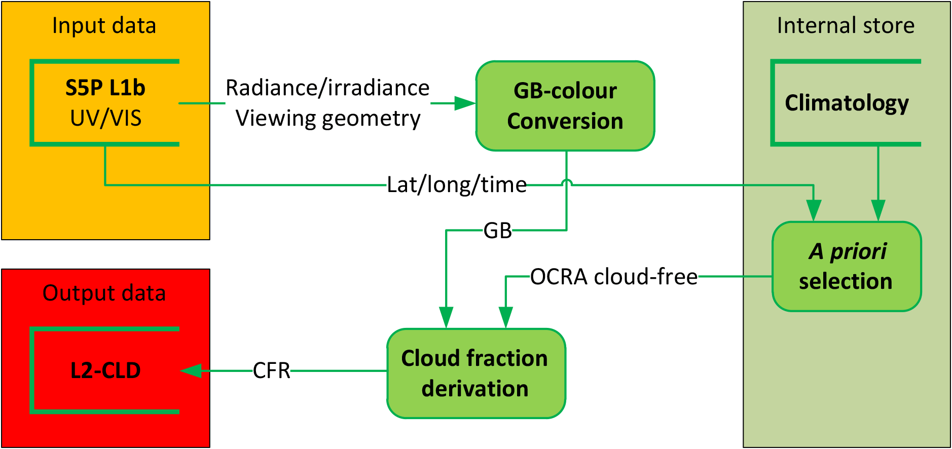
Figure 1Flow diagram for the OCRA algorithm for the retrieval of the radiometric cloud fraction (CFR).
There are three cloud-property algorithms in operational use for the OMI instrument (OMI has no O2 A-band measurements). The first (OMI/Aura Cloud Pressure and Fraction Raman Scattering, or OMCLDRR) uses the cloud screening effect on Fraunhofer filling signatures (due to inelastic rotational Raman scattering) in the region 346–354 nm to derive effective cloud fraction and cloud optical centroid pressure (Joiner and Vasilkov, 2006; Vasilkov et al., 2008; Joiner et al., 2012). This algorithm is based on the mixed Lambertian equivalent reflectivity (MLER) assumption. The second algorithm (OMI/Aura Cloud Pressure and Fraction O2–O2 Absorption, or OMCLDO2) uses reflectances in and around the O2–O2 absorption band near 477 nm (Acarreta et al., 2004; Veefkind et al., 2016); differential optical absorption spectroscopy (DOAS)-retrieved O2–O2 slant columns are compared with simulated look-up table entries to obtain effective cloud fraction and cloud pressure. The third algorithm (OMI/Aura Near UV Aerosol Optical Depth and Single Scattering Albedo, or OMAERUV) derives aerosol optical depth and single-scattering albedo (Torres et al., 2007) from radiances at 354 and 388 nm; the cloud fraction is computed as an intermediate step.
The OCRA cloud fraction determination is based on the comparison between cloud-contaminated measurements and corresponding measurements for the background (cloud-free) surface. A flow chart of the OCRA algorithm is given in Fig. 1, and the algorithm steps are described in the following subsections.
A description of the OCRA algorithm and its application to GOME and GOME-2 data is given in Loyola (1998) and Lutz et al. (2016). For the TROPOMI/S5P application, the new algorithm developments for OCRA are the adaptation to work with two-colour radiances (green and blue: GB) using the UV–VIS spectra instead of the three-colour PMD measurements (red, green, and blue: RGB) in the UV–VIS–NIR region. The reasons for moving from RGB to GB are twofold: first, the TROPOMI UV–VIS and NIR footprints are spatially misaligned, which means that the GB and R colours do not see the exact same footprint, and any misalignment correction would then act as an additional error source in OCRA (see Sect. 5.1). Second, and more importantly, the OMI sensor, which is needed to provide the initial cloud-free reflectance background maps, does not have channels in the red part of the visible spectrum; thus, OMI cannot be used to define a third colour, R. These two considerations dictate the need for a two-colour approach.
3.1 GB colour conversion
The OCRA colour space approach can be applied with three colours (RGB space) or two colours (GB space or RG space). For a given location (x,y), we define the reflectance at wavelength range λi for the footprint of the measurement as
where I(λi) and E0(λi) denote the measured earthshine backscattered radiance and the solar irradiance respectively, and θ0 is the solar zenith angle.
The reflectances used in this algorithm are derived from broadband measurements of backscattered radiance and extraterrestrial solar irradiance covering the spectral range of the GB colour system. The OCRA spectral ranges with TROPOMI/S5P are 405–495 nm for G and 350–395 nm for B.
3.2 OCRA cloud-free background
The core of the algorithm is the construction of a cloud-free composite of multi-temporal (time series of measurements over the same location) reflectances that is independent of atmosphere and solar and viewing angles; this is indicated as the “internal store” in the flowchart of Fig. 1. For the offline creation of cloud-free reflectance composites in the GB case, the green and blue channel reflectances, which are denoted by the letters G and B respectively, are translated into normalised gb colour space via the relations
If M is the set of n normalised multi-temporal measurements over the same location (xy), then a cloud-free (or minimum cloudiness) pixel gbCF∈M is selected using the brightness criterion , for , where W is the white point (1∕2, 1∕2) in the gb-chromaticity diagram. This point refers to a situation where B and G are equal, i.e. where there is no wavelength dependence across the UV–VIS region – this is interpreted as a scene fully covered by cloud. Measurements under cloudy conditions are projected to the white point, and the measurement that is most distant from W is considered to be cloud-free. A cloud-free background, labelled “climatology” in Fig. 1, is constructed by merging cloud-free reflectances ρCF(λi) (corresponding to gbCF) at all locations. It should be noted here that the G and B cloud-free reflectances for a given grid cell are not determined independently as a minimum available reflectance over the whole monthly time range, but rather they are the interdependent reflectances belonging to an individual scene representing the largest distance from the white point in the gb-chromaticity diagram.
At the beginning of the TROPOMI/S5P mission, a monthly cloud-free background data set based on OMI measurements will be used, to be replaced by TROPOMI data as the mission unfolds.
3.3 Cloud fraction derivation
The radiometric cloud fraction fc is determined by examining separations between measured GB reflectances and their corresponding cloud-free composite values:
This equation expresses the distance between actual measurements and the corresponding cloud-free scene in colour space. Scaling factors α(λi=GB) define the upper limit for reflectances under fully cloudy conditions, while offsets β(λi=GB) account for aerosol and other radiative effects in the atmosphere and as a lower limit basically define the cloud-free conditions. The “max” and “min” functions ensure that the cloud fraction is confined to the interval [0, 1].
The scaling and offset factors are determined offline using representative daily global satellite measurements (Lutz et al., 2016). The offsets are the histogram modes from the differences {ρ(λi)−ρCF(λi)}, and the scaling factors are the inverses of the 99th percentile of the cumulative histograms from the differences {ρ(λi)−ρCF(λi)}2. The temporal variability of the offsets and scaling factors is investigated by comparing several daily global histograms at different occasions throughout the year. Since no significant seasonal dependence is apparent, only one set of α and β per colour is used. It should be noted here that the offsets may partially compensate for extremely dark scenes (e.g. shadows) and radiative effects (e.g. absorbing aerosols), but a strict separation of aerosols and clouds is not done by OCRA.
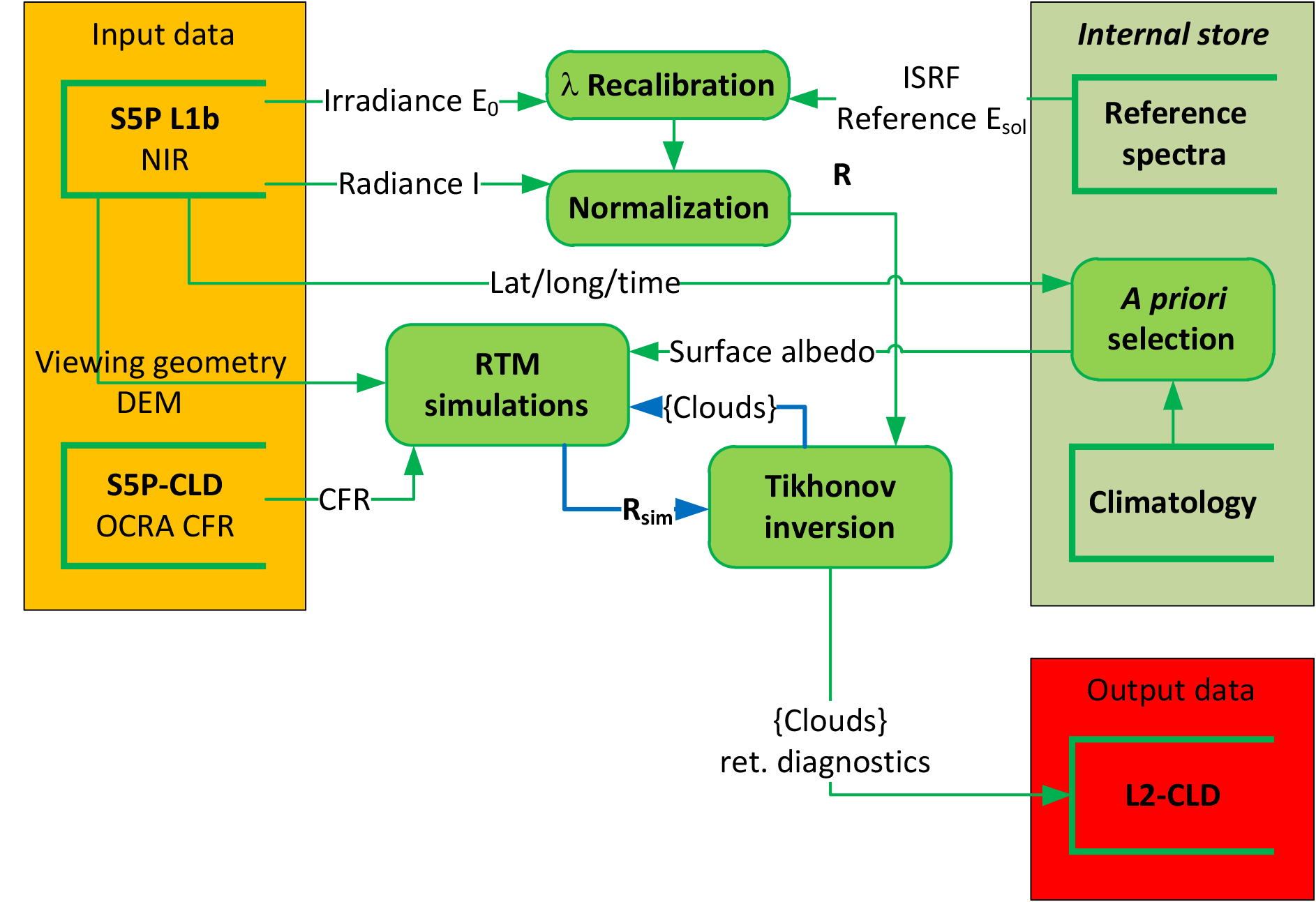
Figure 2Flow diagram for the ROCINN algorithm for retrieval of cloud properties. The blue arrows mark an iterative loop.
3.4 Sun glint flagging
Direct sunlight reflected by the ocean surface may reach the satellite sensor, enhancing the measured signal in a manner which contaminates cloud effects. Sun glint flagging was developed as a component of the operational OCRA algorithm (Loyola, 2011) for GOME-2/MetOp-A, and this treatment was further enhanced using the polarisation Stokes fractions (Lutz et al., 2016) to correct for the sun glint effect. Since TROPOMI does not provide polarisation information, a simplified sun glint flagging procedure will be used instead of this correction. First, those areas that might be affected by sun glint are marked using the viewing geometry conditions of the measurement:
where Θo and Θ are the solar and satellite zenith angles respectively, and φo and φ the solar and satellite azimuth angles (values are given in degrees). A sun glint flag is set whenever the value of “marker” v is larger than a given threshold. This threshold value will be determined dynamically when real TROPOMI data become available; for now, the OMI threshold value of 45 will be used initially.
ROCINN is based on the comparison of measured and simulated radiances in and near the O2 A-band for retrieving the cloud optical thickness, cloud height and albedo. A flow chart of the ROCINN algorithm is given in Fig. 2; the algorithm steps are described in the following subsections.
Previous versions of the ROCINN algorithm for operational processing of GOME (Van Roozendael et al., 2006) and GOME-2 (Loyola et al., 2011) modelled clouds as simple Lambertian surfaces (ROCINN_CRB). The CRB approach was originally developed for GOME (footprint: 320 × 40 km2), where different types of clouds are combined in the large satellite pixels, and errors in the cloud model are compensated (Kokhanovsky et al., 2007), but the limitations of the CRB model are already noticeable with GOME-2 (footprints: 80∕40 × 40 km2), where an intra-cloud correction was developed to compensate for the CRB overestimation of the O3 ghost column (Loyola et al., 2011). For TROPOMI/S5P, with significantly smaller ground pixels (footprint: 7 × 3.5 km2), we have developed the more sophisticated ROCINN_CAL algorithm presented in this paper. In CAL, clouds are modelled as optically uniform layers of scattering water droplets – with this more physically realistic scenario, CAL is expected to be more accurate than CRB, especially for optically thin clouds (Rozanov and Kokhanovsky, 2004). For implementation of CAL model, a detailed description of the parameterisation of liquid water clouds in the forward model is provided in Sect. 4.4.
Another change from older ROCINN versions is with the use of neural networks. In previous ROCINN versions, a neural network was used for solving the inverse function (Loyola et al., 2007), whereas in this version a neural network is used for parameterising the forward model (Sect. 4.4) while the inversion is performed using Tikhonov regularisation (Sect. 4.5). This change in methodology enables us to conduct proper error characterisations for all retrievals (Sect. 4.6).
4.1 Wavelength recalibration
Before we describe ROCINN itself, we remark on the initial wavelength registration (see Fig. 2). The wavelength grid of the measured solar irradiance E0 is recalibrated using a high-resolution solar reference Esol by first dividing the fitting window into sub-windows and computing for each sub-window j a wavelength shift Δλj between E0,j and Esol,j. The solar reference spectrum used for the wavelength calibration is the SAO2010 (https://www.cfa.harvard.edu/atmosphere/links/sao2010.solref.converted) produced for atmospheric measurements in the UV–VIS–NIR by Chance and Kurucz (2010). The calibration is applied on the reference spectrum by using DOAS fit methods as part of the UPAS processor. The recalibrated grid is then established by applying (at each original wavelength point) a shift value computed from a polynomial fit through the Δλj for the various sub-windows. The fitting is achieved for polynomials of a degree of 3 for S5P.
Note that during the inversion (see Sect. 4.5) a wavelength shift for the earthshine spectrum is fitted additionally.
The sun-normalised radiance R(λ) at wavelength λ is then defined as
where I(λ) and E0(λ) denote the measured earthshine backscattered radiance and solar irradiance spectra respectively, with both spectra registered on the recalibrated solar irradiance grid as noted above.
4.2 ROCINN_CAL
For ROCINN with CAL, the total sun-normalised radiance is taken to be a linearly weighted sum of independent radiances Rs for the clear-sky scene and for the cloud-filled scene, with the weighting expressed through the radiometric cloud fraction fc. Both radiance contributions are calculated using standard one-dimensional radiative transfer models (RTMs).
The sun-normalised radiance for a cloudy scene is calculated with the cloud treated as a single scattering layer with geometrical extent characterised by cloud top height Zct and cloud base height Zcb (or alternatively the cloud geometrical thickness . The entire cloud is optically uniform with cloud optical thickness τc, and its scattering properties are determined through Mie-scattering calculations for water droplet particles (microphysical properties are discussed below). In the IPA, we may write sun-normalised CAL simulated radiances as
Here, Θ denotes path geometry (solar and line-of-sight angles), and surface properties are the Lambertian albedo As and lower boundary height Zs.
Radiances for clear-sky and cloudy scenarios are calculated using the VLIDORT (Vector Linearized Discrete Ordinate Radiative Transfer) model (Spurr, 2006), at wavelengths in and adjacent to the O2 A-band. Details of the RTM calculations are given in Sect. 4.4 below.
A complete data set of simulated sun-normalised radiance templates is created offline for an appropriate range of viewing/solar geometries and surface geophysical scenarios, and for various combinations of cloud properties.
The inverse problem uses least-squares fitting with a generalised form of Tikhonov regularisation (details in Sect. 4.5). Retrieval in the O2 A-band with the four-element state vector is an ill-posed problem that requires additional information in order to obtain an inverse solution, as there are only two degrees of freedom for signal (DFS; Schüssler et al., 2014). For ROCINN_CAL, the retrieval state vector is just {τc,Zct} for cloud optical thickness τc and height Zct, a fixed cloud geometrical thickness of 1 km is assumed, and the radiometric cloud fraction fc is taken from OCRA.
4.3 ROCINN_CRB
ROCINN with CRB assumes that clouds are treated as Lambertian reflectors. The sun-normalised CRB simulated radiances are defined as
The retrieval state vector for ROCINN_CRB is {Ac,Zc} for cloud albedo Ac and cloud height Zc; the radiometric cloud fraction fc is again from OCRA.
4.4 Forward model
ROCINN is based on simulated sun-normalised radiances at wavelengths in and around the O2 A-band. Two sets of radiance templates were calculated using the CRB and CAL models. The cloudy-scene sun-normalised radiances were calculated for a multi-layer atmosphere including multiple scattering in all layers. Mie scattering was used to generate cloud optical properties. Details may be found in Schüssler et al. (2014).
Simulated sun-normalised radiances Rsim(λ) are calculated using the vector VLIDORT multiple-scattering multi-layer discrete ordinate RTM (Spurr, 2006); the desired total intensity I will incorporate the effects of polarisation. The incorporation of a vector RTM is necessary not for TROPOMI itself but for the processing of data from GOME, SCIAMACHY, and GOME-2. In addition to the cloud layers, VLIDORT calculations are based on clear-sky optical properties for line absorption by oxygen molecules and Rayleigh scattering by air molecules.
For the line absorption, it is necessary to calculate line-by-line (LBL) radiances (typically at resolution 0.0015 nm for the range 758–771 nm) using line-spectroscopic information for the O2 A-band before convolution with the sensor slit function.
The spectroscopic data are taken from the HITRAN 2012 database (released in June 2013). Absorption cross sections are computed using LBL software from DLR (Schreier and Schimpf, 2001; Schreier, 2011), in which line absorption signatures are accurately modelled with the Voigt profile.
For Mie scattering calculations, we require knowledge of microphysical properties of clouds consisting of liquid water. The droplets are assumed to be randomly distributed within the cloud layer, and any possible inhomogeneity in the cloud is assumed negligible in the current version of CAL model. In addition, we have found that the consistency of cloud models (e.g. CAL or CRB) used in both the cloud and UV–VIS trace gas retrievals is far more critical than the optical properties selected for the RTM simulations of the CAL templates.
The drop size distribution is well approximated by the modified-Gamma size distribution function (Deirmendjian, 1964):
which is parameterised by the mode radius rc in units of microns (µm), and constants α and γ describe the shape of the distribution following Hess et al. (1998). In Eq. (8), C is the normalisation constant. Characteristic values for the low-level cloud (i.e. stratus/cumulus) parameterisation are mode radius rc=4.75 µm and shape parameters α=5 and γ=1.61.
The cloud macro-physical properties (classifications of cloud top height and cloud geometrical thickness) are based on the tables in Wang et al. (2000). Details of this algorithm prototype can be found in Schüssler et al. (2014).
The cloud geometrical thickness is always constant and equal to 1 km; thus, the liquid water path of the cloud is then defined by the total number concentration. A single phase scattering function is used with the extinction cross section for spherical particles obtained by Mie theory (Van de Hulst, 1957; Bohren and Huffman, 1983). The complex refractive index (n+im) of cloud droplets was configured as n=1.33 and for liquid water at 758 nm (Hale and Querry, 1973).
The line-by-line RT calculations in the O2 A-band are computationally very demanding, and this precludes the deployment of online calls to VLIDORT during the processing of TROPOMI data. For this reason, RTM simulations for the range of S5P viewing conditions are performed in advance. Node points for the RTM are created using a “smart sampling” technique (Loyola et al., 2016) that minimises the number of calls to the RTM and at the same time optimally covers the input space. There are many millions of forward-model calculations required; this process is done offline and normally takes several weeks to complete. In the next step, the LBL simulations are convolved with the TROPOMI instrumental spectral response function, and the resulting radiances are used to train a neural network that accurately approximates the RTM template output with a mean average relative error below 1 % over the O2 A-band spectral window for all scene geometries. The node point generation, RTM simulation, and neural-network training are done using the smart sampling and incremental function learning technique (Loyola et al., 2016). The input space (surface properties, cloud properties, and geometries) is not sampled using a set of regular grids, but instead a smart sampling technique (Loyola et al., 2016) is used to optimise the distribution of multi-dimensional points within the (input) state space. The total number of computational nodes was of the order of some hundred thousand. The trained neural network that computes the O2 A-band sun-normalised radiances is used in the UPAS operational environment, and this enables ROCINN retrievals to be done very quickly.
4.5 Inverse model
If x is the state vector comprising possible cloud parameters for retrieval, and b denotes a vector of auxiliary forward-model parameters (surface properties, viewing geometry, etc.), we write the measurement vector as , where F is the forward model and δ is the data error vector. The inverse problem defined by this equation is non-linear and ill-posed, and regularisation is required in order to obtain a solution with physical meaning. The degree to which the problem is ill-posed is partly characterised by the condition number of the Jacobian matrix , where γmax and γmin are the largest and the smallest singular values of K respectively.
In the form of Tikhonov regularisation used here, the regularised solution minimises the objective functional:
Here, α denotes the regularisation parameter, and L is the regularisation matrix (Doicu et al., 2010). The functional is defined with the L2 Euclidean norm. The minimiser for Eq. (9) can be computed with Gauss–Newton methods.
In statistical inversion theory, the Bayesian approach or the optimal estimation method can be regarded as a stochastic version of Tikhonov regularisation. The maximum a posteriori solution coincides with the Tikhonov solution when the state vector x and the noise vector δ are Gaussian random vectors with covariance matrices and Cδ=σ2Im respectively, where σx and σ are the corresponding standard deviations, and In is the identity matrix of size n. In this case, the regularisation parameter α is the ratio of these two variances; that is, .
As noted above, the operational ROCINN algorithm with CAL (or CRB) retrieves two cloud parameters: the cloud top height and cloud optical thickness (or cloud albedo) with the a priori cloud fraction taken from OCRA and the surface albedo from the MERIS black-sky climatology at 760 nm (Popp et al., 2011). Note that the cloud fraction and the surface albedo are included in the state vector with a very strong regularisation (i.e. only very small changes are allowed) in order to improve the fitting. These very small changes refer to the differences between the retrieved value of cloud fraction (and surface albedo) and their corresponding a priori value. The regularisation parameter for cloud fraction and surface albedo is very high (i.e. 2 orders of magnitude higher than that for cloud top height and cloud optical thickness/cloud albedo), and thus these retrieval parameters are always well within 1 % difference from their a priori values. The state vector includes additionally a single wavelength registration shift parameter that takes care of the Doppler effect. The inverse model requires the partial derivatives of the radiances with respect to the state vector elements, and these Jacobians are provided by the forward model.
Convergence is reached when either the residual or incremental changes in the retrieved parameters Δx are smaller than pre-defined values (defaults: 5 × 10⁻³ and 5 × 10⁻⁵), or when the maximum number of iterations (default: 50) is reached. The default value for the regularisation parameter α is 1 × 10⁻⁴.
4.6 Retrieval diagnostics
The equivalence between the Bayesian approach and the method of Tikhonov regularisation enables us to analyse the information content of the signal with respect to the retrieved parameters in a stochastic framework (Schüssler et al., 2014). DFS is a measure of the number of independent pieces of information in the measurement, and it gives the minimum number of parameters which can be used to define a state vector without loss of information. It is defined as the trace of the averaging kernel matrix, which represents the sensitivity of the retrieval to changes in the true state. The DFS can be computed as
where are the singular values of the matrix K.
Another useful criterion for the estimation of the retrieval quality is the Shannon information content (SIC), which is a measure of the incremental gain in information, defined as the entropy difference between the a priori and a posteriori states; the corresponding formula reads as follows:
The accuracy of the regularised solution is represented by the mean square error matrix:
where x† is the exact solution or “true state”, the regularised solution, xa the a priori state vector, Aα the averaging kernel matrix, the generalised inverse, σ the noise standard deviation, α the regularisation parameter, and ε the expected value operator. Further information on the mean square error matrix and Tikhonov regularisation can be found in Doicu et al. (2010).
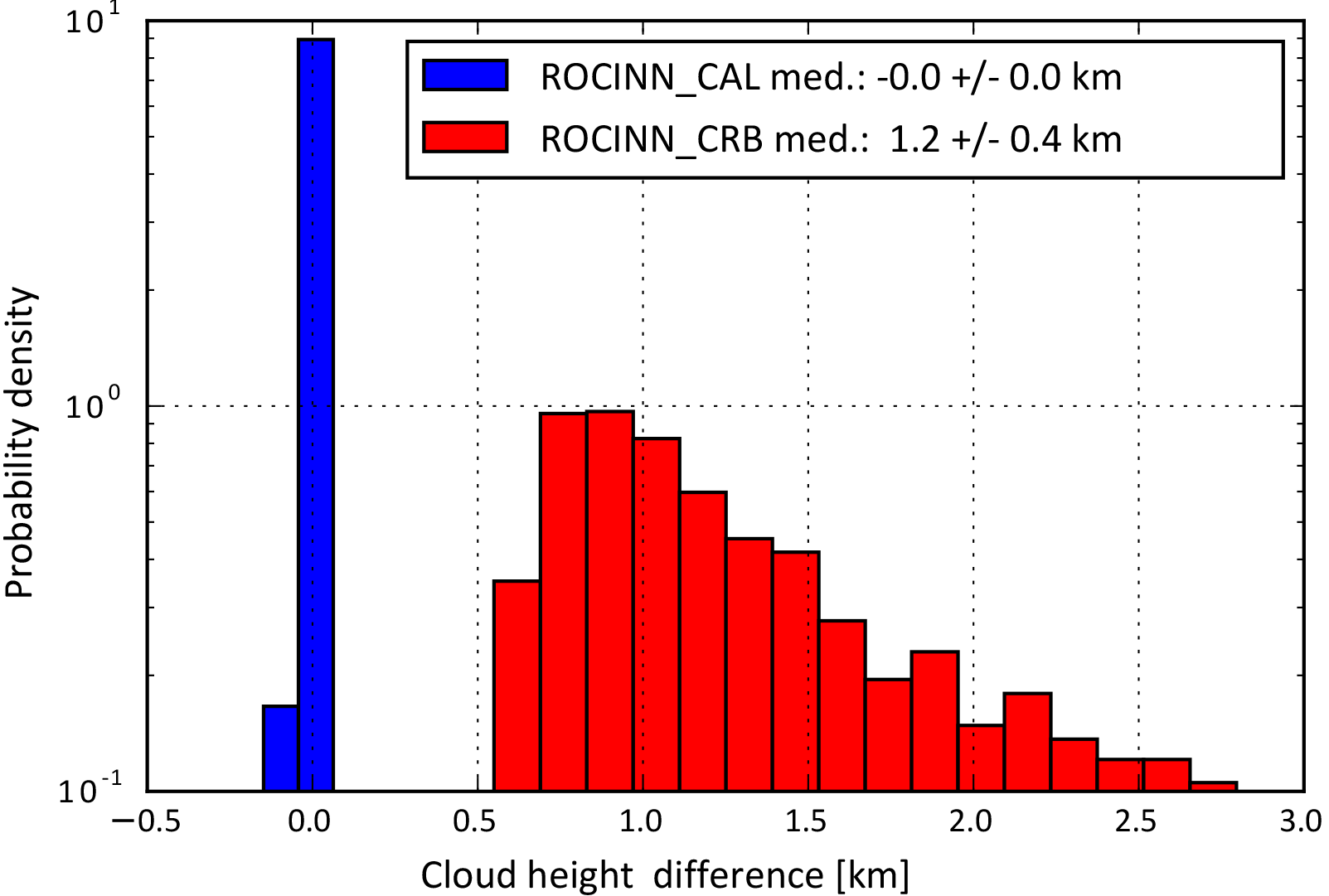
Figure 3Histogram of the absolute differences between the simulated spectra and the cloud height retrievals from ROCINN_CAL and ROCINN_CRB.
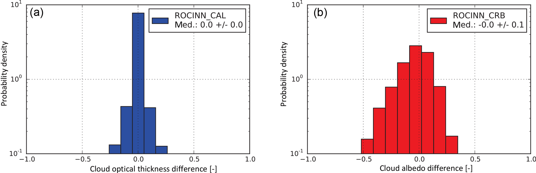
Figure 4Histogram of the absolute differences between the simulated spectra and (a) the cloud optical thickness retrievals from ROCINN_CAL and (b) the cloud albedo retrievals from ROCINN_CRB. The retrieved cloud optical thickness varies from 2 to 50, with the cloud albedo ranging from 0 to 1.
4.7 Retrievals using synthetic spectra
In order to evaluate the performance of the ROCINN retrieval algorithm in TROPOMI/S5P, a data set of synthetic TROPOMI measurements has been created. Synthetic spectra were computed using VLIDORT for a number of different scenarios characterised by various illumination and observation geometries, surface albedo, and cloudiness. In particular, the following input space has been covered using the smart sampling technique: surface height of [0–4] km, surface albedo of [0–1], cloud top height of [2–15] km, cloud optical thickness of [2–50], viewing zenith angle of [0–75] degrees, solar zenith angle of [0–90] degrees, and relative azimuth angle of [0–180] degrees.
In general, these closed-loop ROCINN_CAL retrieval results are excellent; the cloud top height results have no bias. The ROCINN_CRB retrieval was also applied to the same data set of synthetic spectra in order to obtain retrievals of the cloud height and cloud albedo. The results are shown in Fig. 3; as expected, the CRB cloud height is systematically below the simulated cloud top height, with a median difference of 1.2 ± 0.4 km.
Figure 4 shows the correlation from ROCINN_CAL retrievals of cloud optical thickness and ROCINN_CRB retrievals of cloud albedo. The differences in the cloud optical thickness are symmetrical about the zero-bias line, whereas the differences in the cloud albedo are slightly skewed towards negative values.
The accuracy of operational TROPOMI/S5P cloud products retrieved using OCRA and ROCINN is dependent on a number of different error sources.
The most important sources of model parameter uncertainty in ROCINN are errors on the assumed values for cloud fraction and surface albedo. Associated cloud property retrieval errors due to this source are discussed in detail in Schüssler et al. (2014). In summary, the findings are that the cloud top height and cloud optical thickness can be accurately retrieved, even when the cloud fraction is underestimated or overestimated by as much as 20–30 %. On the other hand, the cloud optical thickness retrievals are quite sensitive to uncertainty in the surface albedo. The sensitivity study from Schüssler et al. (2014) showed that deviations of ±10 % in the surface albedo introduce uncertainties of ±5 in the cloud optical thickness retrieval. The cloud retrievals are almost insensitive to cloud geometrical thickness uncertainties. In particular, for deviations of 50 % in the cloud geometrical thickness, the retrieval errors in the cloud top height and cloud optical thickness are lower than 0.4 and 2.0 km respectively. Note that for the accurate retrieval of cloud geometrical thickness from the O2 A-band either multi-angular (Merlin et al., 2016) or high-spectral-resolution (Richardson and Stephens, 2017) measurements are needed.
Errors due to forward-model uncertainty are the hardest to quantify, as these are due to sources such as mathematical discretisation choices and physical simplifications. The most basic assumption is of course the use of a simplified 1-D radiative transfer model as mandated by the IPA. Three-dimensional RTM of atmospheres with clouds is notoriously difficult and time-consuming. With the relatively small TROPOMI spatial footprint, horizontal inhomogeneity in cloud fields will be an important consideration from both a geometrical and the radiation perspective. Some results for a 3-D treatment with clouds have been reported using Monte Carlo models (Marshak and Davis, 2005) and more recently using stochastic RTM methods (Doicu et al., 2014). A detailed analysis of the uncertainties induced by the assumption of IPA with 1-D RTM can be found in a recently published paper (Efremenko et al., 2016); this analysis is the first of its kind to quantify 3-D forward model and retrieval errors in ozone and cloud properties derived from UVN measurements. The results from Efremenko et al. (2016) indicate that the 1-D model generally underestimates radiances in the continuum of the oxygen A-band, while the radiances in the absorption peaks are basically the same. As a consequence, the cloud optical thickness is systematically slightly underestimated by retrievals based on the IPA, whereas the cloud top height retrievals are generally unaffected. That paper also shows that use of the IPA leads to systematic errors in the retrieved ozone height-resolved partial columns.
The selection of a single liquid water cloud for the parametrisation of clouds is a good approximation for describing light scattering by liquid cloud droplets in the atmosphere. The probability of a photon scattering in the forward direction is larger when a light beam at NIR wavelengths interacts with a cloud droplet with effective radius of a few microns, and thus the phase functions of water clouds can be well modelled by Mie theory (Kokhanovsky, 2004). However, Mie theory is not adequate to describe scattering by larger droplets of complex arbitrary shapes (e.g. ice crystals), and consequently the phase function of ice clouds cannot be modelled by spherical polydispersions (Takano and Liou, 1989, 1995; Kokhanovsky, 2004). The associated errors can be assessed using radiative transfer simulations based on ice scattering phase functions as input to the ROCINN_CAL retrieval. The cloud optical thickness varies from 5 to 30, and the cloud height from 6 to 10 km. We have found that the retrieved cloud top height is almost unaffected, with an average error smaller than 2 % for all cases considered. The errors on optical thickness are of the order of 1 % for thick clouds and are larger for thin clouds with retrieved values of 6.06 compared to input optical thickness of 5.0.
Another source of error in the forward model is the simple assumption of a single cloud layer, since multi-layered clouds are often present in reality. The most common such situation in the atmosphere occurs with two cloud layers: one low-level cloud and a second mid-level cloud (Wang et al., 1999). With a view to obtaining estimates of the uncertainties of ROCINN to such double-layer conditions, we have simulated the radiances for a double-cloud-layer model consisting of a mid-level cloud deck (altocumulus/altostratus) on top of the low-level cloud. The upper layer has a top height of 6 km, geometrical thickness of 2 km, and an optical thickness of 10 (Warren et al., 1985).
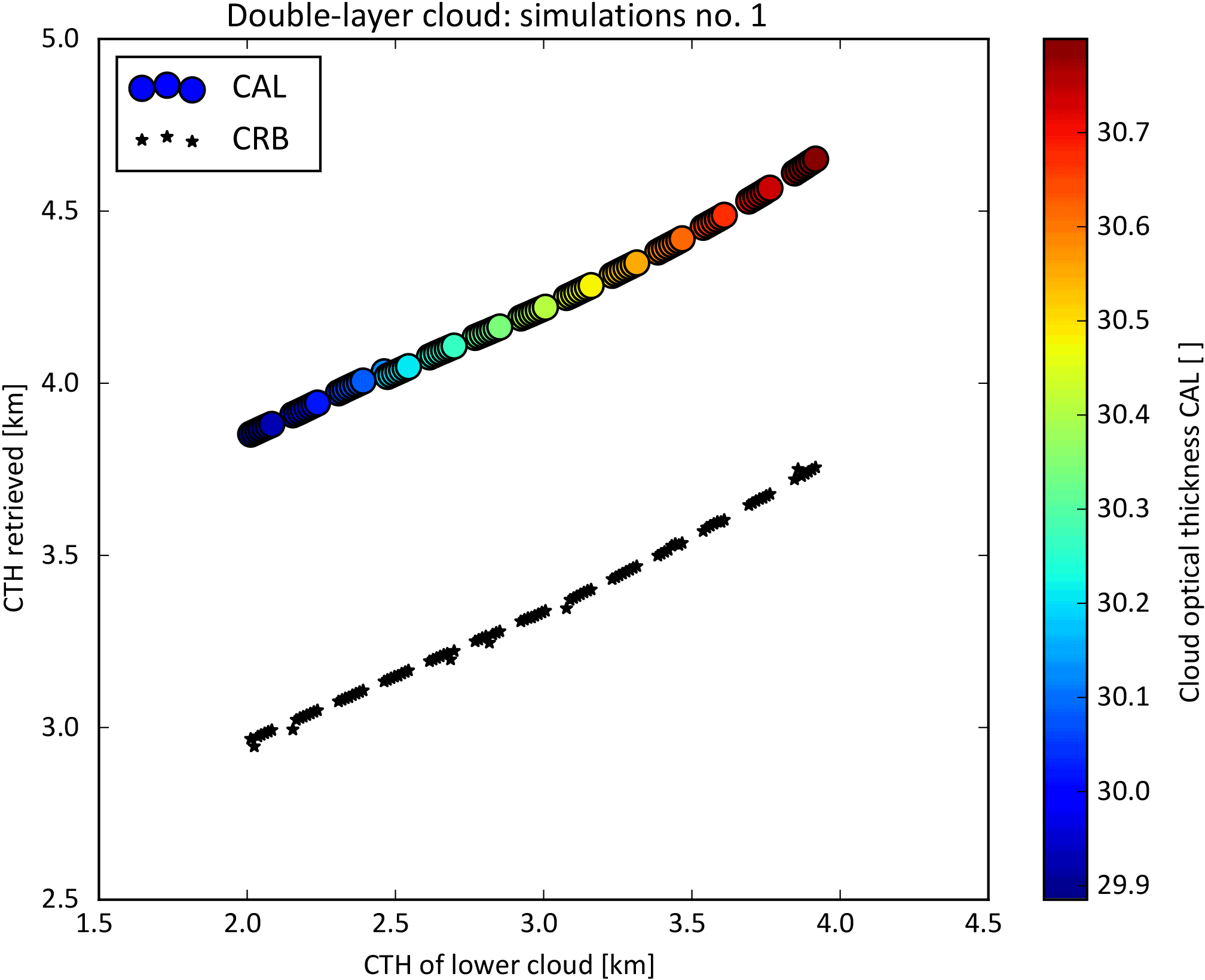
Figure 5ROCINN-retrieved cloud properties for the first group of simulations (i.e. a low cloud with cloud optical thickness of 25, cloud geometrical thickness of 1 km, and cloud top height in the range 2–4 km, plus a mid-level cloud having cloud optical thickness of 10, cloud top height of 6 km, and cloud geometrical thickness of 2 km).
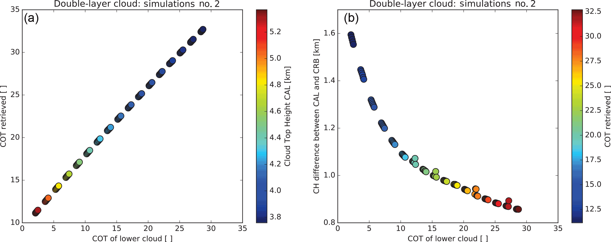
Figure 6(a) Retrieved cloud top height and cloud optical thickness from ROCINN_CAL for the second group of simulations (i.e. a low cloud with cloud top height of 2 km, cloud geometrical thickness of 1 km, and cloud optical thickness in the range 2–30, plus a mid-level cloud with cloud optical thickness of 10, cloud top height of 6 km, and cloud geometrical thickness of 2 km). (b) Differences in cloud height retrieval between CRB and CAL as a function of the optical thickness of the low cloud.
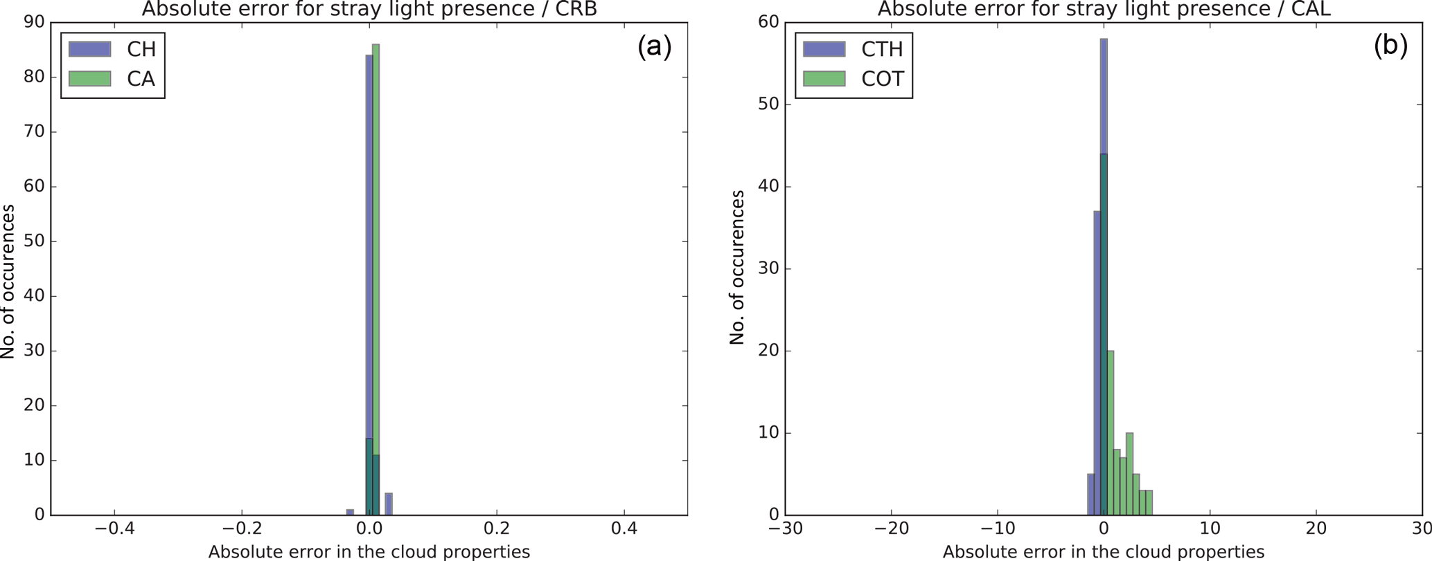
Figure 7Absolute errors in the cloud properties due to the presence of stray light: (a) cloud height and cloud albedo errors for CRB and (b) cloud top height and cloud optical thickness errors for CAL.
The first group of simulation tests is based on a situation with a thick low cloud having cloud optical thickness of 25 and a cloud top height varying from 2 to 4 km below the mid-level cloud (see Fig. 5). We found that the retrieved cloud optical thickness is not affected by the position of the lower cloud, and the retrieved value was approximately 30. The accuracy of the cloud top height retrieval seems to depend on the separation distance between the two clouds (cloud bottom height of the upper cloud minus cloud top height of the lower cloud). When the lower cloud is well separated from the upper cloud, the error in the retrieved cloud top height becomes larger (e.g. when the lower cloud has a top of 2 km, ROCINN_CAL retrieves a cloud top height of approximately 4 km; when the lower cloud has a top of 3.5 km, the retrieved value is 4.4 km). In the second group of simulations, the lower cloud has a top height of 2 km and optical thickness varying from 2 to 30 (see Fig. 6). Now, the mean retrieved cloud top height from ROCINN_CAL was 4.3 km but with variations between 3.8 and 5.3 km. The large cloud top height values were retrieved for an optically thin lower cloud. However, in reality, with atmospheric scenes with two-layered clouds, it is common that the lower cloud is thicker than the upper one (Warren et al., 1985; Wang et al., 1999). In such cases (lower cloud optical thickness > 20), the cloud top height retrieved with ROCINN_CAL is below 4 km. The retrieved cloud optical thickness is absolutely dependent on the cloud optical thickness of the lower cloud. For thick low clouds (cloud optical thickness of 25–30), ROCINN retrieves a cloud optical thickness which basically corresponds to the cloud optical thickness of the lower cloud but with a small contribution of the second upper cloud (retrieved cloud optical thickness of 29–32).
In Fig. 5, for all the simulations that were performed, the cloud height retrieved from CRB was about 0.8 km lower than that retrieved from CAL. Moreover, as seen in Fig. 6, the cloud height retrieved from ROCINN_CRB is even less sensitive to the two-layered cloud when the lower cloud is optically thinner. For very thin low clouds (with an optical thickness of ∼ 2), the difference between retrieved cloud heights from CAL and from CRB increased to as much as 1.6 km. Nevertheless, as stated above, when two cloud layers co-exist in the same atmospheric column, usually the low-level cloud is optically thicker than the mid-level cloud (Warren et al., 1985; Wang et al., 1999).
From the TROPOMI calibration exercise, results have indicated that instrumental errors such as signal-to-noise and radiometric uncertainties in the UVN region are relatively small, although stray-light issues were identified in the NIR band (Loots et al., 2018). Both the errors induced on retrieved cloud properties due to NIR stray light and the precise knowledge of the slit function response functions will be assessed when the instrument provides measurements from space. However, in the absence of real measurements, the impact of stray light in the oxygen A-band has been initially assessed using a flat error of 1.2 % in the radiances (Loots et al., 2018). The absolute errors on the cloud properties can be seen in Fig. 7 for both CRB and CAL models. The retrievals from ROCINN_CRB are almost unaffected by the presence of stray light, with a mean error of 0.003 km for cloud height and a mean error of 0.007 for cloud albedo. These errors induced in the cloud parameter retrievals by ROCINN_CAL are higher, with a mean cloud top height error of 0.3 km and a mean error of 1.0 for cloud optical thickness.
5.1 Coregistration inhomogeneity flag
An important source of error is the spatial misregistration between the UV–VIS and NIR bands from TROPOMI. The combination of information from different spectral bands is not as straightforward as it appears, since the spatial regions covered by the ground pixels from different spectral bands do not match exactly. One method for combining information from different bands is by means of the TROPOMI coregistration mapping tables, which contain the fractions of overlapping areas between the source and target pixels (Sneep, 2015). For combinations based on OCRA UV bands 3, 4, and 5 and ROCINN NIR band 6, a static coregistration table suffices. However, this method implies a smoothing of the source band products.
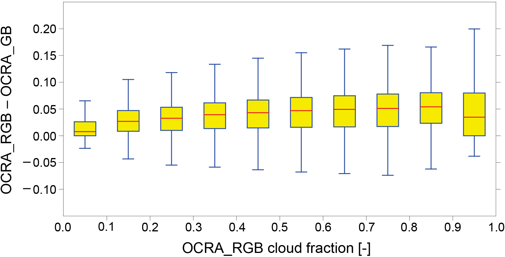
Figure 8Box-and-whisker plot of the OCRA cloud fraction difference using RGB and GB colours retrieved using GOME-2 data from 1 July 2012. The yellow boxes show the interquartile range, and median values are indicated as red lines. The overall median difference is 0.025.
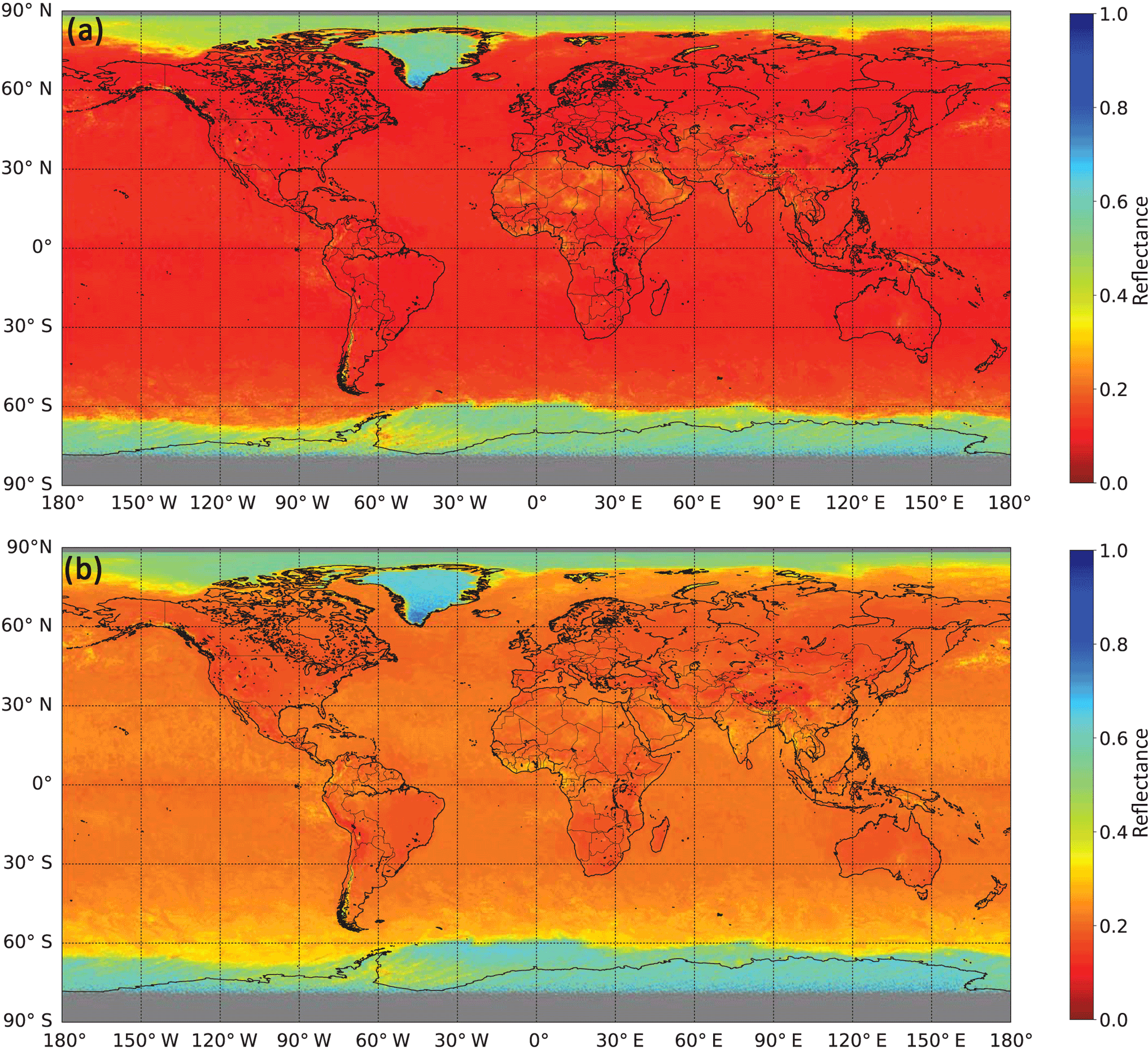
Figure 9OCRA cloud-free background for G (a) and B (b) reflectances calculated using OMI data from the month of August for the years 2005–2007.
For this purpose, a cloud coregistration inhomogeneity flag (CCIF) will be included in the S5P cloud products. This is determined as follows. First, a cloud coregistration inhomogeneity parameter (CCIP) is defined as the weighted averaged gradient of cloud fractions:
where the weights ωij correspond to the coregistration mapping values between UV bands (source, index i) and the NIR band (target, index j). The CCIF is defined as
where p is a fixed threshold which has been set to 0.4 as the baseline, following extensive testing using the VIIRS (Visible/Infrared Imager and Radiometer Suite) cloud product on board the Suomi NPP (NPOESS Preparatory Project) resampled to the TROPOMI spatial grid.
The operational OCRA and ROCINN cloud algorithms presented in this paper have been fully implemented and tested in the TROPOMI/S5P operational processor UPAS under development at DLR. The resulting output files will follow the same netCDF format structure used for all the S5P L2 products. The main outputs are the cloud products retrieved with OCRA and ROCINN_CAL, while the ROCINN_CRB retrievals are to be reported in the detailed results group. For more information, the reader is referred to the S5P Cloud Product User Manual (Pedergnana et al., 2016).
In this section we present the results obtained through application of the TROPOMI/S5P cloud algorithms implemented in UPAS to measurements from OMI and GOME-2.
6.1 Comparison of OCRA_RGB and OCRA_GB using GOME-2
The two-colour OCRA_GB model was tested against the three-colour OCRA_RGB model. The overall median cloud fraction difference is 0.026 and the mean 0.032 for a single day of GOME-2A measurements from 1 July 2012. For cloud fractions smaller than 0.1 the median and mean differences are 0.007 and 0.015 respectively.
Figure 8 shows the cloud fraction differences in a box-and-whisker plot. The bottom, inside band, and top of the box are the first, median, and third quartiles of the differences respectively.
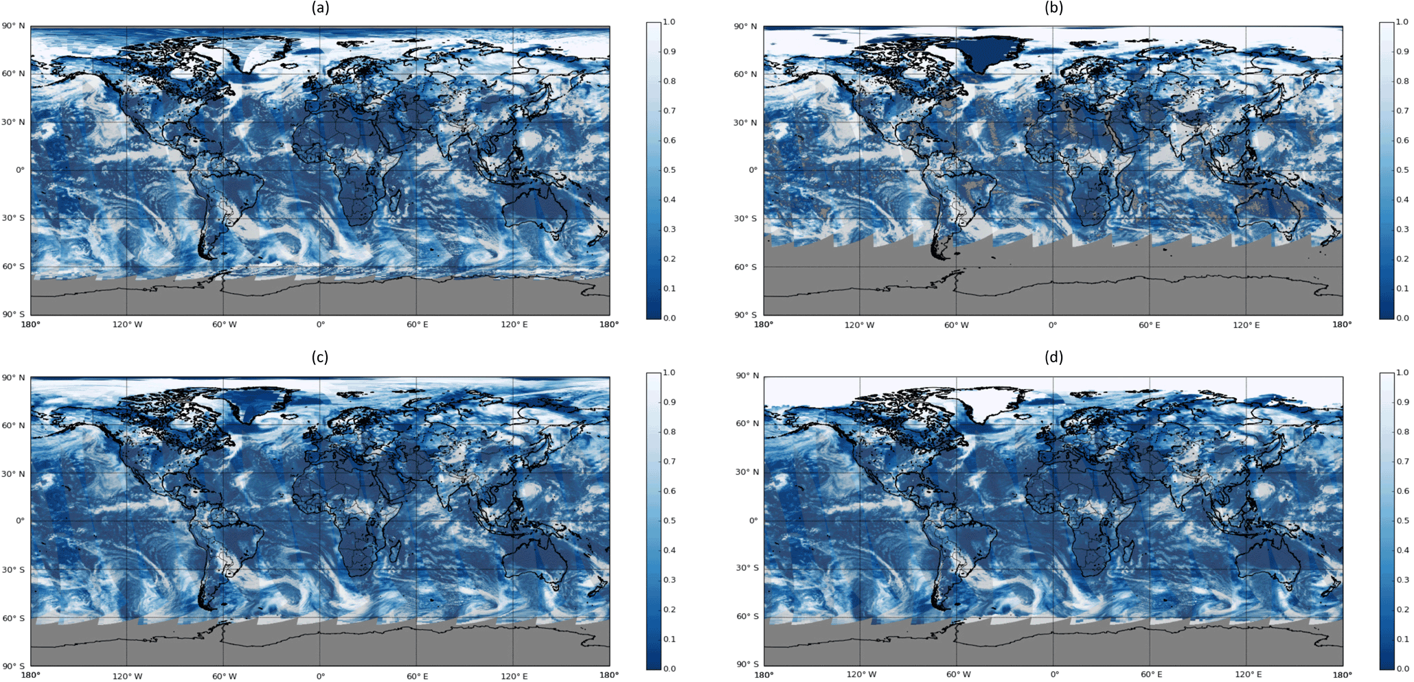
Figure 10Cloud fraction retrieved with (a) OCRA, (b) OMAERUV, (c) OMCLDO2, and (d) OMCLDRR from OMI measurements on 16 July 2005.
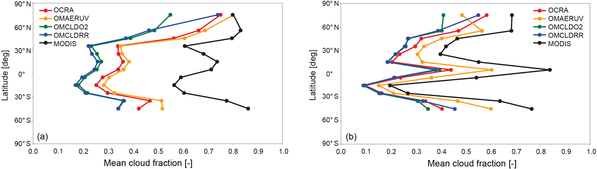
Figure 11Comparison of cloud fraction zonal means for results from the four OMI algorithms as seen in Fig. 10 and from the MODIS measurements regridded to the corresponding OMI ground pixels. The left panel shows only measurements over ocean, while the right panel shows only measurements over land.
6.2 Comparison of OCRA with OMI and MODIS cloud fractions
As part of the S5P project we have adapted the OCRA algorithm to the OMI sensor (the precursor of TROPOMI).
OMI is a nadir-viewing push-broom spectrometer observing solar backscatter radiation in the ultraviolet and visible wavelength range up to 500 nm (Levelt et al., 2006). The swath width is 2600 km on the ground, encompassing more than 60 across-track pixels. The highest spatial resolution of 13 × 24 km2 (in normal mode) is achieved for the nadir pixels. OMI was launched in 2004 on the NASA Aura satellite platform.
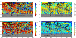
Figure 12Cloud top height (a) and cloud optical thickness (b) retrieved with ROCINN_CAL, cloud height (c) and cloud albedo (d) retrieved with ROCINN_CRB from GOME-2A measurements on 1 July 2012. The cloud height is displayed in metres, and a logarithmic scale is used for the optical thickness.
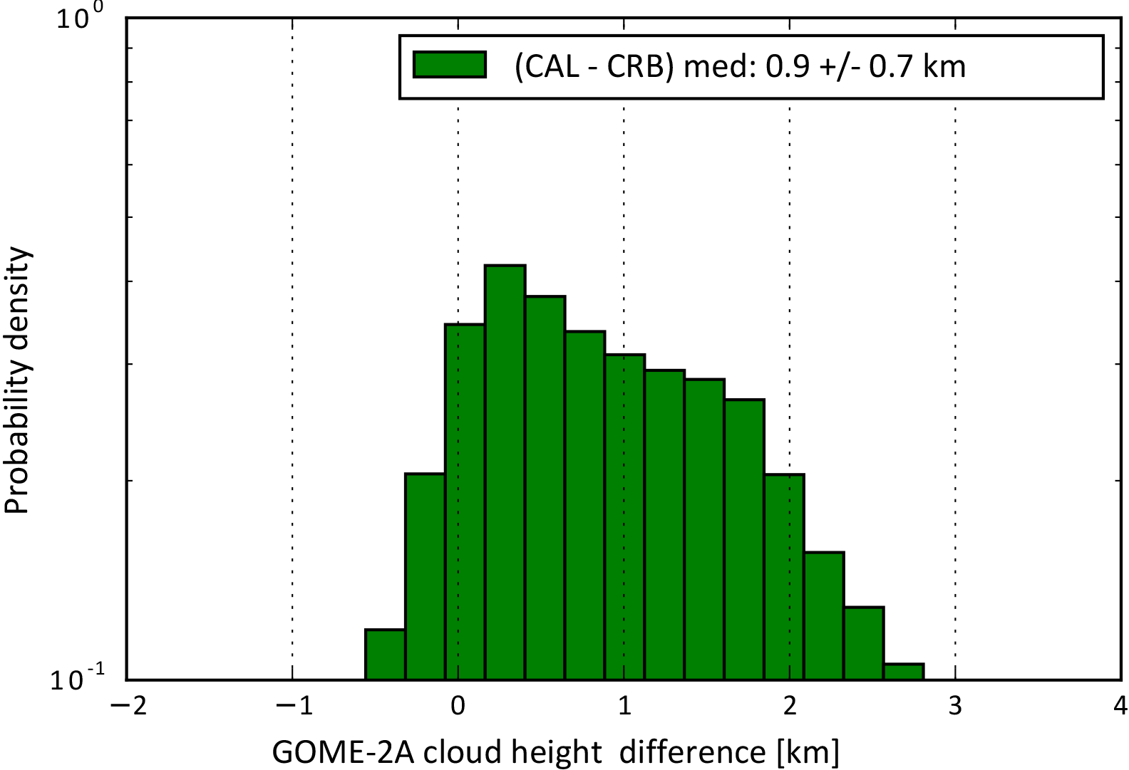
Figure 13Histogram of the absolute differences between the GOME-2A cloud heights derived from ROCINN_CAL and ROCINN_CRB as seen in Fig. 12.
The first step is the calculation of a monthly OCRA cloud-free background data set as described in Sect. 3.2; this was based on 3.5 years of OMI measurements from January 2005 to June 2008. The OMI cloud-free background data set for the month of August is shown in Fig. 9. Note that OMI is extremely stable, with almost no instrument degradation – this facilitates significantly the calculation of the OCRA cloud-free backgrounds.
The temporal resolution is 1 month; i.e. for a given grid cell, all measurements from a given month are aggregated in order to reflect seasonal surface variations. Finally, all data from the years 2005, 2006, 2007, and 2008 are considered for the final monthly maps. The spatial grid resolution is 0.2∘ latitude by 0.4∘ longitude. The cloud-free reflectance value for any given time and geolocation is found via linear interpolation between the two adjacent monthly cloud-free maps. This linear interpolation between monthly maps was found to give the best trade-off between the necessity to have as many measurements as possible per grid cell in order to ensure a cloud-free situation (i.e. a long timescale is desired) and the requirement to be sensitive to rapid changes in the surface conditions such as snowfall or melting (i.e. a short timescale is desired).
Secondly, the scaling and offset factors are computed following the procedure described in Sect. 3.3. The resulting scaling factors are αB=2.88 and αG=2.14, and the offset factors are βB=0.0138 and βG=0.0180.
For the comparison with MODIS, we used the following cloud products:
-
The OMAERUV product, provided by O. Torres. The cloud fraction is an ancillary product from the absorbing aerosol index algorithm based on OMI radiances at 388 and 354 nm (Torres et al., 2007).
-
The OMCLDO2 product version 2.0, provided by P. Veefkind. The cloud fraction of this product is based on the OMI O2–O2 absorption feature around 477 nm (Veefkind et al., 2016).
-
The OMCLDRR product, taken from the OMMYCLD product version 003 (OMI/Aura and MODIS/Aqua Merged Cloud Product 1-Orbit L2 Swath 13 × 24 km2 V003, Greenbelt, MD, USA, Goddard Earth Sciences Data and Information Services Center (GES DISC), last access: 26 October 2016). This OMI cloud fraction is derived at 354 nm, where the contribution of Raman scattering is minimal.
-
The MODIS product co-located to OMI footprints from the OMMYDCLD product version 003. This product provides the OMI/Aura and MODIS/Aqua merged cloud products. No MODIS/Terra data are incorporated here. Since both Aura and Aqua are part of the A-train, the overpass times are comparable (the separation between Aura and Aqua is 8 min).
Figure 10 shows the global cloud maps obtained with OCRA, OMAERUV, OMCLDO2, and OMCLDRR from OMI measurements on 16 July 2005; the four algorithms generate similar cloud features.
A quantitative comparison of the zonal mean cloud fractions from OMI and those derived with MODIS is presented in Fig. 11. The UV sensors are less sensitive to optically thin clouds than thermal infrared sensors; as expected, MODIS generates larger cloud fractions compared to those from OMI. The cloud fractions of OMCLDO2 and OMCLDRR are similar because both algorithms assume a fixed cloud albedo or reflectance of 0.8 for the retrieval, but overall the cloud albedo is significantly smaller (e.g. Lelli et al., 2012, report a mean global cloud albedo value of 0.63 based on GOME data from 1996–2003), and therefore the retrieved effective cloud fractions are significantly smaller than the MODIS geometrical cloud fractions. On the other hand, OCRA and OMAERUV do not need to assume a fixed cloud albedo, and their retrieved cloud fractions are larger than those from OMCLDO2 and OMCLDRR. OCRA and OMAERUV report cloud fraction values more representative of the radiometric cloud fraction based on top-of-atmosphere radiances measured by the instrument. We should emphasise here that a direct comparison between the MODIS geometric cloud fraction and the OMI-derived radiometric or effective cloud fractions should be treated with caution.
6.3 Comparison of ROCINN cloud top height and optical thickness from GOME-2
In preparation for S5P we have applied the ROCINN_CAL algorithm to GOME-2, and in this section we present for the first time the resulting cloud parameter retrievals.
GOME-2 is a nadir-viewing optical spectrometer that senses Earth's backscattered radiance and solar irradiance at UV–VIS–NIR wavelengths in the range 240–790 nm (Munro et al., 2016). The nominal full GOME-2 swath has a width of 1920 km in the direction perpendicular to the flight direction, and a single scan line has an extension of 40 km in the flight direction. The ground pixels have a spatial resolution of 80 × 40 km2. In addition, broadband PMDs provide an eightfold higher spatial resolution, i.e. 10 × 40 km2 for a selection of 15 spectral windows. Currently there are two GOME-2 operational sensors on board the EUMETSAT MetOp-A and MetOp-B satellites launched in 2006 and 2012 respectively; both GOME-2 sensors are operated in tandem, providing global measurements on a daily basis. A third GOME-2 sensor on board MetOp-C will be launched in 2018.
The VLIDORT line-by-line RTM simulations described in Sect. 4.4 are convolved with the GOME-2 instrumental spectral response functions, and these results are then used to train a neural network that accurately approximates the O2 A-band reflectances (Loyola et al., 2016). As noted in Sect. 4.5, the ROCINN cloud top height and optical thickness are retrieved using the Tikhonov inversion, taking as input the OCRA cloud fraction computed from the GOME-2 PMD measurements (Lutz et al., 2016).
Figure 12 shows the global cloud maps obtained with ROCINN_CAL and ROCINN_CRB from GOME-2A (GOME-2 on MetOp-A) measurements taken on 1 July 2012. As expected from the retrievals with synthetic data (Sect. 4.7) the cloud height retrieved using ROCINN_CRB is smaller than that retrieved using ROCINN_CAL; the CRB model retrieves the centroid of the cloud and not the cloud top (Joiner et al., 2012). The cloud optical thickness from ROCINN_CAL nicely correlates with the cloud albedo from ROCINN_CRB.
The histogram of absolute differences between the GOME-2A cloud heights on 1 July 2012 obtained with ROCINN_CAL and ROCINN_CRB is presented in Fig. 13. The CRB model underestimates the cloud top height with a median difference of 0.92 ± 0.75 km. These results are consistent with the retrievals obtained using synthetic data from Sect. 4.7.
The diagnostic quantities DFS and SIC for the test case of 1 July 2012 were found to lie in the ranges 1.2–4 and 2–11 respectively for ROCINN_CAL. These values are lower than those obtained for ROCINN_CRB (DFS between 2.1 and 4.3, SIC in the range 4–17), showing that the CAL-retrieved cloud quantities depend more on the a priori information.
We have presented the latest versions of the retrieval algorithms OCRA and ROCINN to be used for the generation of the operational TROPOMI/S5P cloud products: cloud fraction, cloud top height (pressure), and optical thickness (albedo).
In UPAS, special effort has been directed to optimising the run-time performance of the algorithms in order to cope with the “big data” expected from TROPOMI (around 21 million ground pixels daily, with 1.5 million pixels per orbit). The operational cloud retrievals are extremely fast and accurate: the OCRA cloud fraction is computed using a simple expression (Eq. 3), while the time-consuming generation of the cloud-free composite is done offline. Similarly the complex and computationally expensive line-by-line RTM calculations needed for the ROCINN retrieval of cloud top height and optical thickness are replaced by fast artificial neural networks trained using the smart sampling and incremental function learning techniques (Loyola et al., 2016).
The OCRA and ROCINN algorithms are integrated in the S5P operational processor UPAS for the generation of near-real-time and offline products. In this paper we have shown that UPAS cloud properties retrieved from OMI and GOME-2 measurements provide a good basis for anticipated retrievals from TROPOMI measurements themselves.
The algorithms presented in this paper will be used during the S5P commissioning phase. The operational TROPOMI cloud products will be validated using ground-based measurements of cloud radar and microwave radiometer instruments available at CloudNet stations and using cloud products from VIIRS on board the Suomi NPP satellite of NASA/NOAA; the S5P orbit will trail 5 min behind Suomi NPP.
A number of future algorithm developments are planned once the TROPOMI data become available after the S5P launch: the spatial misregistration between the UV–VIS and NIR bands will be characterised and the possibility of a correction will be investigated, the effects of TROPOMI stray light in NIR on the cloud retrievals will be analysed, and a cloud-free background data set based on TROPOMI/S5P will be generated once the first full year of measurements becomes available; this will replace the initial cloud-free background data based on OMI.
The OCRA and ROCINN cloud parameters will be used for enhancing the accuracy of the operational TROPOMI/S5P trace gas products total ozone (Loyola et al., 2017), formaldehyde, and sulfur dioxide (Theys et al., 2016). OCRA and ROCINN will be also used for the generation of operational cloud products from the geostationary Copernicus atmospheric composition mission Sentinel-4 (S4). In this way, cloud products from atmospheric composition missions S5P and S4 will be consistent, and together they will extend for the next 2 decades the unique UVN cloud data record (Loyola et al., 2010) initiated over 20 years ago with GOME/ERS-2.
The operational Copernicus Sentinel-5 Precursor products, including the cloud properties described in this paper, are generated at DLR and will be freely available via ESA.
The authors declare that they have no conflict of interest.
This article is part of the special issue “TROPOMI on Sentinel-5 Precursor: data products and algorithms”. It is not affiliated with a conference.
Two co-authors are no longer affiliated with DLR: Sebastián Gimeno García (now at EUMETSAT, Darmstadt, Germany) and Olena Schüssler.
Thanks to the S5P L2WG cloud verification team, in particular Holger Sihler (MPIC) and Luca Lelli (IUP-UB) for helpful comments. Thanks to Omar Torres (NASA), Joanna Joiner (NASA), and Pepijn Veefkind (KNMI) both for providing the OMI and MODIS cloud data used in our OCRA comparisons and for a number of helpful discussions. Thanks to KNMI/NASA for the OMI level 1 products and EUMETSAT for the GOME-2 level 1 products used in this paper.
This work has been performed in the framework of the TROPOMI/S5P project. We acknowledge financial support from Bayerisches Staatsministerium für Wirtschaft und Medien, Energie und Technologie (grant 0703/89373/15/2013); from DLR programmatic (S5P KTR 2 472 046) for the S5P algorithm development; and from the ESA S5P L2WG project (contract no.: 4000107711/13/NL/IB) for the S5P operational processor development.
Finally, the authors thank three anonymous reviewers for their fruitful
input and suggestions which have helped to improve this manuscript.
The article processing charges for this open-access
publication were covered by a Research
Centre of the Helmholtz Association.
Edited by: Joanna Joiner
Reviewed by: three anonymous referees
Acarreta, J. R., de Haan, J. F., and Stammes, P.: Cloud pressure retrieval using the O2-O2 absorption band at 477 nm, J. Geophys. Res., 109, D05204, https://doi.org/10.1029/2003JD003915, 2004.
Ahmad, Z., Bhartia, P. K., and Krotkov, N.: Spectral properties of backscattered UV radiation in cloudy atmospheres, J. Geophys. Res, 109, D01201, https://doi.org/10.1029/2003JD003395, 2004.
Boersma K., Eskes, H., and Brinksma E.: Error analysis for tropospheric NO2 retrieval from space, J. Geophys. Res, 109, D44311, https://doi.org/10.1029/2003JD003962, 2004.
Bohren, C. F. and Huffman, D. R.: Absorption and scattering by small particles, Wiley, NY, 1983.
Chance, K. and Kurucz, R. L.: An improved high-resolution solar reference spectrum for earth's atmosphere measurements in the ultraviolet, visible, and near infrared, J. Quant. Spectrosc. Ra., 111, 1289–1295, 2010.
Deirmendjian, D.: Scattering and polarization properties of water clouds and hazes in the visible and infrared, Appl. Opt., 3, 187–196, 1964.
Doicu, A., Trautmann, T., and Schreier, F.: Numerical Regularization for Atmospheric Inverse Problems, Berlin, Springer Verlag, 2010.
Doicu, A., Efremenko, D., Loyola, D., and Trautmann, T.: Discrete ordinate method with matrix exponential for stochastic radiative transfer in broken clouds, J. Quant. Spectrosc. Ra., 138, 1–16, 2014.
du Piesanie, A., Piters, A. J. M., Aben, I., Schrijver, H., Wang, P., and Noël, S.: Validation of two independent retrievals of SCIAMACHY water vapour columns using radiosonde data, Atmos. Meas. Tech., 6, 2925–2940, https://doi.org/10.5194/amt-6-2925-2013, 2013.
Efremenko, D. S., Schüssler, O., Doicu, A., and Loyola, D.: A stochastic cloud model for cloud and ozone retrievals from UV measurements, J. Quant. Spectrosc. Ra., 184, 167–179, 2016.
Grzegorski, M., Wenig, M., Platt, U., Stammes, P., Fournier, N., and Wagner, T.: The Heidelberg iterative cloud retrieval utilities (HICRU) and its application to GOME data, Atmos. Chem. Phys., 6, 4461–4476, https://doi.org/10.5194/acp-6-4461-2006, 2006.
Hale, G. M. and Querry, M. R.: Optical constants of water in the 200-nm to 200-µm wavelength region, Appl. Opt., 12, 555–563, 1973.
Hao, N., Koukouli, M. E., Inness, A., Valks, P., Loyola, D. G., Zimmer, W., Balis, D. S., Zyrichidou, I., Van Roozendael, M., Lerot, C., and Spurr, R. J. D.: GOME-2 total ozone columns from MetOp-A/MetOp-B and assimilation in the MACC system, Atmos. Meas. Tech., 7, 2937–2951, https://doi.org/10.5194/amt-7-2937-2014, 2014.
Hess, M., Koepke, P., and Schult, I.: Optical Properties of Aerosols and Clouds: The Software Package OPAC, Bull. Am. Met. Soc, 79, 831–844, 1998.
Heue, K.-P., Coldewey-Egbers, M., Delcloo, A., Lerot, C., Loyola, D., Valks, P., and van Roozendael, M.: Trends of tropical tropospheric ozone from 20 years of European satellite measurements and perspectives for the Sentinel-5 Precursor, Atmos. Meas. Tech., 9, 5037–5051, https://doi.org/10.5194/amt-9-5037-2016, 2016.
Joiner, J. and Vassilkov, A. P.: First results from the OMI rotational Raman scattering cloud pressure algo-rithm, IEEE T. Geosci. Remote, 44, 1272–1282, 2006.
Joiner, J., Vasilkov, A. P., Gupta, P., Bhartia, P. K., Veefkind, P., Sneep, M., de Haan, J., Polonsky, I., and Spurr, R.: Fast simulators for satellite cloud optical centroid pressure retrievals; evaluation of OMI cloud retrievals, Atmos. Meas. Tech., 5, 529–545, https://doi.org/10.5194/amt-5-529-2012, 2012.
Koelemeijer, R. and Stammes, P.: A fast method for retrieval of cloud parameters using oxygen A-band measurements from the Global Ozone Monitoring Experiment, J. Geophys. Res., 106, 3475–3490, 2001.
Kokhanovsky, A.: Optical properties of terrestrial clouds, Earth-Sci. Rev., 64, 189–241, 2004.
Kokhanovsky, A. A. and Rozanov, V. V.: The uncertainties of satellite DOAS total ozone retrieval for a cloudy sky, Atmos. Res., 87, 27–36, https://doi.org/10.1016/j.atmosres.2007.04.006, 2008.
Kokhanovsky, A. A., Mayer, B., Rozanov, V. V., Wapler, K., Lamsal, L. N., Weber, M., Burrows, J. P., and Schumann, U.: The influence of broken cloudiness on cloud top height retrievals using nadir observations of backscattered solar radiation in the oxygen A-band, J. Quant. Spectrosc. Ra., 103, 460–477, https://doi.org/10.1016/j.jqsrt.2006.06.003, 2007.
Krotkov, N. A., Bhartia, P. K., Herman, J. R., Ahmad, Z., and Fioletov, V.: Satellite estimation of spectral surface UV irradiance 2: Effect of homogeneous clouds and snow, J. Geophys. Res., 106, 11743–11759, 2001.
Kuze, A. and Chance, K. V.: Analysis of Cloud-Top Height and Cloud Coverage from Satellites Using the O2A and B Bands, J. Geophys. Res., 99, 14481–14491, 1994.
Lelli, L., Kokhanovsky, A. A., Rozanov, V. V., Vountas, M., Sayer, A. M., and Burrows, J. P.: Seven years of global retrieval of cloud properties using space-borne data of GOME, Atmos. Meas. Tech., 5, 1551–1570, https://doi.org/10.5194/amt-5-1551-2015, 2012.
Lelli, L., Weber, M., and Burrows, J. P.: Evaluation of SCIAMACHY ESA/DLR Cloud Parameters Version 5.02 by Comparisons to Ground-Based and Other Satellite Data, Front. Environ. Sci., 4, 1–14, https://doi.org/10.3389/fenvs.2016.00043, 2016.
Levelt, P. F., van den Oord, G. H. J., Dobber, M. R., Malkki, A., Visser, H., de Vries, J., Stammes, P., Lundell, J. O. V., and Saari, H.: The Ozone Monitoring Instrument, IEEE T. Geosci. Remote, 44, 1093–1101, 2006.
Lindfors, A. V., Kujanpää, J., Kalakoski, N., Heikkilä, A., Lakkala, K., Mielonen, T., Sneep, M., Krotkov, N. A., Arola, A., and Tamminen, J.: The TROPOMI surface UV algorithm, Atmos. Meas. Tech. Discuss., https://doi.org/10.5194/amt-2017-210, in review, 2017.
Liu, X., Newchurch, M., Loughman, R., and Bhartia P.K.: Errors resulting from assuming opaque Lambertian clouds in TOMS ozone retrieval, J. Quant. Spectrosc. Ra., 85, 337–365, 2004.
Loots, E., Kleipool, Q., Ludewig, A., and Rozemeijer, N.: NIR out-of-spectral-band stray-light analysis report, S5P-KNMI-OCAL-0152-RP, issue 0.1, in review, 2018.
Loyola, D. and Ruppert, T.: A new PMD cloud-recognition algorithm for GOME, ESA Earth Observation Quarterly, 58, 45–47, 1998.
Loyola, D., Thomas, W., Livschitz, Y., Ruppert, T., Albert, P., and Hollmann, R.: Cloud properties derived from GOME/ERS-2 backscatter data for trace gas retrieval, IEEE T. Geosci. Remote, 45, 2747–2758, 2007.
Loyola, D., Thomas, W., Spurr, R., and Mayer, B.: Global patterns in daytime cloud properties derived from GOME backscatter UV-VIS measurements, Int. J. Remote Sens., 31, 4295–4318, https://doi.org/10.1080/01431160903246741, 2010.
Loyola, D., Koukouli, M., Valks, P., Balis, D., Hao, N., Van Roozendael, M., Spurr, R., Zimmer, W., Kiemle, S., Lerot, C., and Lambert, J.-C.: The GOME-2 Total Column Ozone Product: Retrieval Algorithm and Ground-Based Validation, J. Geophys. Res., 116, D07302, https://doi.org/10.1029/2010JD014675, 2011.
Loyola, D., Pedergnana, M., and Gimeno García, S.: Smart sampling and incremental function learning for very large high dimensional data, Neural Networks, 78, 75–87, 2016.
Loyola, D., et al.: The near-real-time total ozone retrieval algorithm from TROPOMI onboard Sentinel-5 Precursor, Atmos. Meas. Tech. Discuss., in preparation, 2018.
Lutz, R., Loyola, D., Gimeno García, S., and Romahn, F.: OCRA radiometric cloud fractions for GOME-2 on MetOp-A/B, Atmos. Meas. Tech., 9, 2357–2379, https://doi.org/10.5194/amt-9-2357-2016, 2016.
Marshak, A. and Davis, A. B. (Eds.): 3D Radiative Transfer in Cloudy Atmospheres, Series Physics of Earth and Space Environments, Springer-Verlag, Berlin, Heidelberg, 2005.
Merlin, G., Riedi, J., Labonnote, L. C., Cornet, C., Davis, A. B., Dubuisson, P., Desmons, M., Ferlay, N., and Parol, F.: Cloud information content analysis of multi-angular measurements in the oxygen A-band: application to 3MI and MSPI, Atmos. Meas. Tech., 9, 4977–4995, https://doi.org/10.5194/amt-9-4977-2016, 2016.
Munro, R., Lang, R., Klaes, D., Poli, G., Retscher, C., Lindstrot, R., Huckle, R., Lacan, A., Grzegorski, M., Holdak, A., Kokhanovsky, A., Livschitz, J., and Eisinger, M.: The GOME-2 instrument on the Metop series of satellites: instrument design, calibration, and level 1 data processing – an overview, Atmos. Meas. Tech., 9, 1279–1301, https://doi.org/10.5194/amt-9-1279-2016, 2016.
Pedergnana, M., Loyola D., Apituley A., Sneep M., and Veefkind P.: Sentinel-5 precursor/TROPOMI – Level 2 Product User Manual – Cloud Properties, S5P-L2-DLR-PUM-400I available at: https://sentinel.esa.int/web/sentinel/technical-guides/sentinel-5p/appendices/references and http://www.tropomi.eu/documents/level-2-products (last access: 22 December 2017), 2016.
Popp, C., Wang, P., Brunner, D., Stammes, P., Zhou, Y., and Grzegorski, M.: MERIS albedo climatology for FRESCO + O2 A-band cloud retrieval, Atmos. Meas. Tech., 4, 463–483, https://doi.org/10.5194/amt-4-463-2011, 2011.
Richardson, M. and Stephens, G. L.: Information content of OCO-2 oxygen A-band channels for retrieving marine liquid cloud properties, Atmos. Meas. Tech. Discuss., https://doi.org/10.5194/amt-2017-314, in review, 2017.
Rozanov, V. and Kokhanovsky, A.: Semi-analytical cloud retrieval algorithm as applied to the cloud top altitude and the cloud geometrical thickness determination from top-of-atmosphere reflectance measurements in the oxygen A-band, J. Geophys. Res., 109, D05202, https://doi.org/10.1029/2003JD004104, 2004.
Schreier, F.: Optimized implementations of rational approximations for the Voigt and complex error function, J. Quant. Spectrosc. Ra., 112, 1010–1025, 2011.
Schreier, F. and Schimpf, B.: A new efficient line-by-line code for high resolution atmospheric radiation computations incl. derivatives, in: IRS 2000: Current Problems in Atmospheric Radiation, edited by: Smith, W. L. and Timofeyev, Y., Hampton, VA, USA, A. Deepak Publishing, 381–384, 2001.
Schüssler, O., Loyola, D., Doicu, A., and Spurr, R.: Information Content in the Oxygen A-band for the Retrieval of Macrophysical Cloud Parameters, IEEE T. Geosci. Remote, 52, 3246–3255, 2014.
Sihler, H., Wagner, T., Sneep, M., Stammes, P., Wang, P., and Lelli, L.: Clouds, in: S5P/TROPOMI Science Verification Report, edited by: Richter, A. and the Verification Teams, issue: 2.1, available at: https://sentinel.esa.int/web/sentinel/user-guides/sentinel-5p-tropomi/document-library (last access: 22 December 2017), 2015.
Sneep, M.: Sentinel-5 precursor inter-band coregistration mapping tables, S5P-KNMI-L2-0129-TN, issue 4.0.0, 2015.
Spurr, R. J. D.: VLIDORT: A linearized pseudo-spherical vector discrete ordinate radiative transfer code for forward model and retrieval studies in multilayer multiple scattering media, J. Quant. Spectrosc. Ra., 102, 316–42, https://doi.org/10.1016/j/jqsrt.2006.05.005, 2006.
Stammes, P., Sneep, M., de Haan J. F., Veefkind, J. P., Wang, P., and Levelt, P. F.: Effective cloud fractions from the Ozone Monitoring Instrument: Theoretical framework and validation, J. Geophys. Res., 113, D16S38, https://doi.org/10.1029/2007JD008820, 2008.
Stengel, M., Stapelberg, S., Sus, O., Schlundt, C., Poulsen, C., Thomas, G., Christensen, M., Carbajal Henken, C., Preusker, R., Fischer, J., Devasthale, A., Willén, U., Karlsson, K.-G., McGarragh, G. R., Proud, S., Povey, A. C., Grainger, R. G., Meirink, J. F., Feofilov, A., Bennartz, R., Bojanowski, J. S., and Hollmann, R.: Cloud property datasets retrieved from AVHRR, MODIS, AATSR and MERIS in the framework of the Cloud_cci project, Earth Syst. Sci. Data, 9, 881–904, https://doi.org/10.5194/essd-9-881-2017, 2017.
Takano, Y. and Liou, K.-N.: Solar radiative transfer in cirrus clouds: 1. Single scattering and optical properties of hexagonal ice crystals, J. Atmos. Sci., 46, 3–19, 1989.
Takano, Y. and Liou, K.-N.: Solar radiative transfer in cirrus clouds: 1. Light scattering of irregular ice crystals, J. Atmos. Sci., 452, 818–837, 1995.
Theys, N., De Smedt, I., Yu, H., Danckaert, T., van Gent, J., Hörmann, C., Wagner, T., Hedelt, P., Bauer, H., Romahn, F., Pedergnana, M., Loyola, D., and Van Roozendael, M.: Sulfur dioxide retrievals from TROPOMI onboard Sentinel-5 Precursor: algorithm theoretical basis, Atmos. Meas. Tech., 10, 119–153, https://doi.org/10.5194/amt-10-119-2017, 2017.
Torres, O., Tanskanen, A., Veihelman, B., Ahn, C., Braak, R., Bhartia, P. K., Veefkind, P., and Levelt, P.: Aerosols and surface UV products from OMI observations: An overview, J. Geophys. Res., 112, D24S47, https://doi.org/10.1029/2007JD008809, 2007.
Torres, O., Jethva, H., and Bhartia, P. K.: Retrieval of aerosol optical depth above clouds from OMI observations: Sensitivity analysis and case studies, J. Atmos. Sci., 69, 1037–1053, https://doi.org/10.1175/JAS-D-11-0130.1, 2011.
Valks, P., Pinardi, G., Richter, A., Lambert, J.-C., Hao, N., Loyola, D., Van Roozendael, M., and Emmadi, S.: Operational total and tropospheric NO2 column retrieval for GOME-2, Atmos. Meas. Tech., 4, 1491–1514, https://doi.org/10.5194/amt-4-1491-2011, 2011.
van Deelen, R., Hasekamp, O. P., van Diedenhoven, B., and Landgraf, J.: Retrieval of cloud properties from near-ultraviolet, visible, and near-infrared satellite-based Earth reflectivity spectra: A comparative study, J. Geophys. Res., 113, D12204, https://doi.org/10.1029/2007JD009129, 2008.
Van de Hulst, H. C.: Light scattering by small particles, Wiley, NY, 1957.
van Diedenhoven, B., Hasekamp, O. P., and Landgraf, J.: Retrieval of cloud parameters from satellite-based reflectance measurements in the ultraviolet and the oxygen A-band, J. Geophys. Res., 112, D15208, https://doi.org/10.1029/2006JD008155, 2007.
Van Roozendael, M., Loyola, D., Spurr, R., Balis, D., Lambert, J-C., Livschitz, Y., Valks, P., Ruppert, T., Kenter, P., Fayt, C., and Zehner C.: Ten years of GOME/ERS-2 total ozone data: the new GOME Data Processor (GDP) Version 4: I. Algorithm Description, J. Geophys Res., 111, D14311, https://doi.org/10.1029/2005JD006375, 2006.
Vasilkov, A., Joiner, J., Spurr, R., Bhartia, P. K., Levelt, P., and Stephens, G.: Evaluation of the OMI cloud pressures derived from rotational Raman scattering by comparisons with other satellite data and radiative transfer simulations, J. Geophys. Res., 113, D15S19, https://doi.org/10.1029/2007JD008689, 2008.
Veefkind, J. P., Aben, I., McMullan, K., Förster, H., de Vries, J., Otter, G., Claas, J., Eskes, H. J., de Haan, J.F., Kleipool, Q., van Weele, M., Hasekamp, O., Hoogeven, R., Landgraf, J., Snel, R., Tol, P., Ingmann, P., Voors, R., Kruizinga, B., Vink, R., Visser, H., and Levelt, P. F.: TROPOMI on the ESA Sentinel-5 Precursor: A GMES mission for global observations of the atmospheric composition for climate, air quality and ozone layer applications, Remote Sens. Environ., 120, 70–83, https://doi.org/10.1016/j.rse.2011.09.027, 2012.
Veefkind, J. P., de Haan, J. F., Sneep, M., and Levelt, P. F.: Improvements to the OMI O2–O2 operational cloud algorithm and comparisons with ground-based radar–lidar observations, Atmos. Meas. Tech., 9, 6035–6049, https://doi.org/10.5194/amt-9-6035-2016, 2016.
Wagner, T., Beirle, S., Deutschmann, T., Grzegorski, M., and Platt, U.: Dependence of cloud properties derived from spectrally resolved visible satellite observations on surface temperature, Atmos. Chem. Phys., 8, 2299–2312, https://doi.org/10.5194/acp-8-2299-2008, 2008.
Wang, J., Rossow, W. B., Uttal, T., and Rozendaal, M., Variability of cloud vertical structure during ASTEX observed from a combination of rawinsonde, radar, ceilometer, and satellite, Mon. Weather Rev., 127, 2484–2502, 1999.
Wang, J., Rossow, W. B., and Zhang, Y.: Cloud Vertical Structure and Its Variations from a 20-Yr Global Rawinsonde Dataset, J. Clim., 13, 3041–3056, 2000.
Wang, P., Stammes, P., van der A, R., Pinardi, G., and van Roozendael, M.: FRESCO+: an improved O2 A-band cloud retrieval algorithm for tropospheric trace gas retrievals, Atmos. Chem. Phys., 8, 6565–6576, https://doi.org/10.5194/acp-8-6565-2008, 2008.
Warren, S. G., Hahn, C. J., and London, J.: Simultaneous occurrence of different cloud types, J. Clim. Appl. Meteorol., 24, 658–667, 1985.