the Creative Commons Attribution 4.0 License.
the Creative Commons Attribution 4.0 License.
 | 19 Jul 2018
Estimating observation and model error variances using multiple data sets
Therese Rieckh
In this paper we show how multiple data sets, including observations and models, can be combined using the “three-cornered hat” (3CH) method to estimate vertical profiles of the errors of each system. Using data from 2007, we estimate the error variances of radio occultation (RO), radiosondes, ERA-Interim, and Global Forecast System (GFS) model data sets at four radiosonde locations in the tropics and subtropics. A key assumption is the neglect of error covariances among the different data sets, and we examine the consequences of this assumption on the resulting error estimates. Our results show that different combinations of the four data sets yield similar relative and specific humidity, temperature, and refractivity error variance profiles at the four stations, and these estimates are consistent with previous estimates where available. These results thus indicate that the correlations of the errors among all data sets are small and the 3CH method yields realistic error variance profiles. The estimated error variances of the ERA-Interim data set are smallest, a reasonable result considering the excellent model and data assimilation system and assimilation of high-quality observations. For the four locations studied, RO has smaller error variances than radiosondes, in agreement with previous studies. Part of the larger error variance of the radiosondes is associated with representativeness differences because radiosondes are point measurements, while the other data sets represent horizontal averages over scales of ∼ 100 km.
- Article
(4586 KB) - Full-text XML
- BibTeX
- EndNote


Estimating the error characteristics of any observational system or model is important for many reasons. Not only are these errors of scientific interest; they are also important for data assimilation systems and numerical weather prediction. In many modern data assimilation schemes, observations of a given type are weighted proportionally to the inverse of their error variance (Desroziers and Ivanov, 2001).
Kuo et al. (2004) and Chen et al. (2011) used the difference between radio occultation (RO) observations and short-range model forecasts to estimate the error of the RO observations, using the concept of apparent or perceived errors, defined by
where XAE is the apparent error of the RO observation and XRO and Xfcst are the RO observations and model forecast values, respectively.
The error variance of the apparent error is given by
where n is the number of samples of observed and modeled RO at the same location and time.
The relationship between the apparent error variance , the observational error variance , and the forecast error variance is given by
where the COVerr term is the error covariance between the observations and the forecasts. If the error variance of the forecast is estimated independently, the observational error variance can be estimated from the apparent error variance, under the assumption that the observational errors are uncorrelated with the forecast errors (in which case the COVerr term in Eq. 3 is zero).
We note that the apparent errors are the same as the O − B (observation minus background) or innovations as used in data assimilation methods and studies (Chen et al., 2011).
As discussed by Kuo et al. (2004) and Chen et al. (2011), the forecast error variance can be estimated by two alternative methods, the National Meteorological Center (NMC) method (Parrish and Derber, 1992) or the Hollingsworth and Lönnberg (1986) method. Kuo et al. (2004) used both methods to estimate the observational errors of RO refractivity using the National Centers for Environmental Prediction (NCEP) Aviation Model (AVN). They found that the estimated radiosonde (RS) observations had larger errors than the RO observations, due in part to representativeness errors of the RS, which provide in situ point measurements, whereas the model data were larger-scale horizontal averages similar to those of the RO data. Chen et al. (2011) used the NMC method and Weather and Research Forecast Model (WRF) to estimate the forecast error variance and then the RO refractivity error variance.
In this paper, we estimate the error variances of multiple data sets using the “three-cornered hat” (3CH) method (Gray and Allan, 1974). Unlike the apparent-error method, this method does not require independent estimates of the error variance of a forecast; it uses the differences between combinations of three data sets. The 3CH method is described in Appendix A along with the closely related “triple-collocation method” (Stoffelen, 1998). The data sets may be either different model or observational data, and estimates of the error variances of all the data sets are computed by the method. We compare three observational data sets (two versions of RO retrievals and radiosondes) and two model data sets at four locations in the tropics and subtropics to estimate the error variances of all five data sets. We find that the results are consistent with each other and with previous error estimates, where available.
We use five data sets from an entire year (2007) in this study. Rieckh et al. (2018) extensively studied the properties of these data sets and their daily variability over 2007 in the tropical and subtropical western Pacific. They are described in more detail there but are summarized briefly here for convenience.
We chose 2007 for the year of our study because the number of COSMIC (Constellation Observing System for Meteorology, Ionosphere, and Climate) RO observations was near a maximum at this time. Because the primary interest in Rieckh et al. (2018) was the evaluation of water vapor observations and model analyses in challenging tropical and subtropical environments, we chose one RS station in the deep tropics and three Japanese stations in the subtropics. Because of our focus on water vapor, we carry out the analysis from 1000 to 200 hPa.
2.1 ERA-Interim
The ERA-Interim (hereafter ERA) reanalysis is a global model reanalysis produced by the European Centre for Medium-Range Weather Forecasts (ECMWF) (Dee et al., 2011). Information about the current status of ERA-Interim production, availability of data online, and near-real-time updates of various climate indicators derived from ERA-Interim data can be found at https://www.ecmwf.int/en/research/climate-reanalysis/reanalysis-datasets/era-interim.
We use the ERA analysis product, which assimilates both RS and RO data for the entire year of 2007; hence some correlation of model, RS, and RO errors is likely. However, there are many other observations going into the ERA reanalysis, and model correlations with any one observational data set are likely to be small.
2.2 NCEP Global Forecast System (GFS)
The Global Forecast System (GFS) is a forecast model produced by the National Centers for Environmental Prediction (NCEP). Data are available for download through the NOAA National Operational Model Archive and Distribution System (NOMADS). Forecast products and more information on GFS are available at https://www.ncdc.noaa.gov/data-access/model-data/model-datasets/global-forcast-system-gfs.
The GFS assimilated RS observations for the entire year 2007 but began assimilating RO data on 1 May 2007, along with many other changes to the model and analysis system (Cucurull and Derber, 2008; Kleist et al., 2009). Thus the GFS and RS and RO errors are also likely correlated to some degree. However, we computed vertical profiles of the correlation coefficients for RO and GFS refractivity, temperature, specific humidity, and relative humidity in the 2 months before and after 1 May 2007, when the GFS started assimilating RO data, and found little differences, so the error correlations between RO and GFS are likely small.
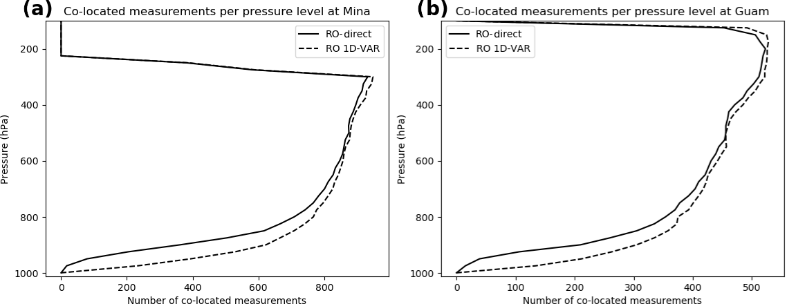
Figure 1Number of co-located measurements for (a) Mina and (b) Guam. These are also the sample numbers in the calculations of the estimated error variances for the data sets. When using the RO 1D-VAR, the number of co-locations is slightly higher than for the RO-direct throughout the profile due to the way the 1D-VAR is computed.
2.3 Radio occultation observations
The RO observations used in this study are re-processed data obtained from the UCAR COSMIC Data Analysis and Archive Center (CDAAC). Two methods for estimating the temperature and water vapor from the RO refractivity are used. In the direct method, the GFS temperature is used in the Smith and Weintraub (1953) equation
to compute water vapor pressure e from the observed refractivity N and GFS temperature T.
A one-dimensional variational (1D-VAR) method is also used to estimate T and e from N. The 1D-VAR method uses an a priori state of the atmosphere (background profile) and an observed RO N profile to minimize a quadratic cost function. At CDAAC, an ERA-Interim profile is used as a background, which is interpolated to the time and location of the RO observation (accounting for tangent point drift during the occultation). The humidity retrieval allows an error for both T and e but only a very small error for bending angle/refractivity. Specific humidity q is then computed from the derived e.
2.4 Radiosonde observations
RS data from Guam and three Japanese stations are used in this comparison. The RS data are given on nine main pressure levels between 1000 and 200 hPa, plus additional levels if atmospheric conditions are variable. The four stations use the following sensors: Guam: VIZ/Sippican B2; Ishigakijima: Meisei; Minamidaitōjima: Vaisala RS92; and Naze: Meisei. They are launched twice daily in the hour before noon and midnight, UTC.
Guam is located in the deep tropics at 13.7∘ N, 144.8∘ E. Ishigakijima (hereafter called Ishi), Minamidaitōjima (hereafter called Mina), and Naze are located relatively close together in the western Pacific subtropics south of Japan and northeast of Taiwan:
-
Naze (Kagoshima Prefecture): 28.4∘ N, 129.4∘ E
-
Mina (Okinawa Prefecture): 25.6∘ N, 131.5∘ E
-
Ishi (Okinawa Prefecture): 24.2∘ N, 124.5∘ E
2.5 Co-location of the data sets
The locations of the four radiosonde stations are chosen for the comparisons. We use RO observations that are located within 600 km and 3 h of the radiosonde launches. CDAAC provides GFS and ERA profiles that are already linearly interpolated in space and time to the RO location and time. These interpolated profiles, along with the RO observations, were corrected for their time and spatial differences from the radiosonde data using a model correction algorithm (Gilpin et al., 2018). Thus the effect of spatial and temporal differences among the data sets is expected to be minor.
The refractivity for the radiosonde and model data is computed from Eq. (5) using the pressure, temperature, and water vapor from these data. Normalized differences are computed for all combinations of the data sets (RO–ERA, RO–GFS, GFS–ERA, RS–ERA, RS–GFS, RS–RO), where RO is either the RO-direct or the RO 1D-VAR data. The ERA annual mean for 2007 at each RS station is used to normalize the differences in the data sets associated with that station. We consider the differences among all data sets for four variables: refractivity (N), temperature (T), specific humidity (q), and relative humidity (RH).
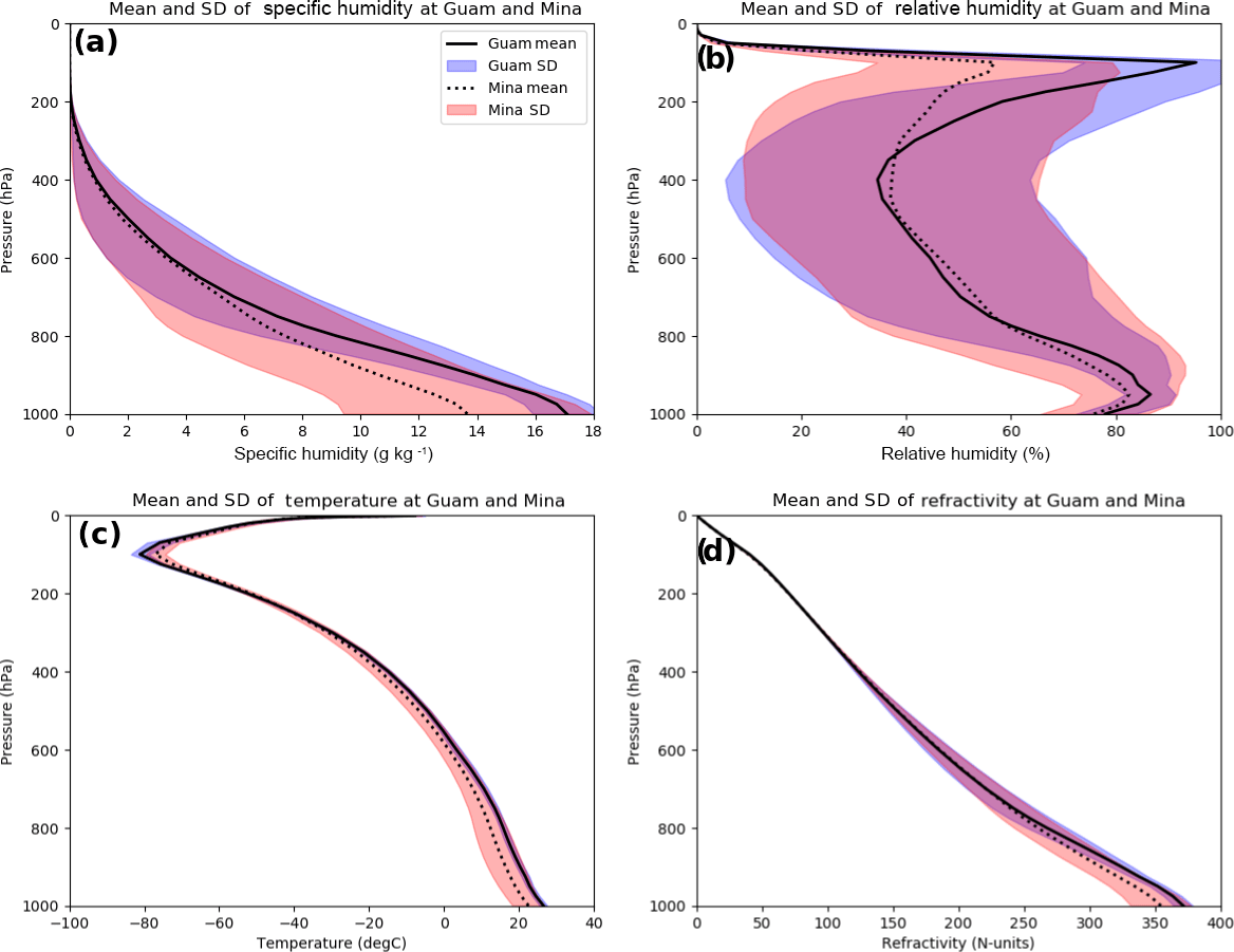
Figure 2The mean ERA profiles over 2007 at Guam and Mina of specific humidity q (a), relative humidity RH (b), temperature T (c), and refractivity N (d). The standard deviations about the mean profiles are indicated by the shading.
2.6 Number of samples
The number of samples is limited by the number of RO observations that are within the co-location criteria of 3 h and 600 km. Figure 1 shows the number of data samples per pressure level that meet these criteria during 2007 at Mina (the numbers at Ishi and Naze are similar) and Guam. The sharp cutoff on the top of the profiles is due to limited RS data availability at high altitudes. The smooth transition to lower numbers at the bottom results from a decrease in the number of RO observations with lower altitudes in the mid- and lower troposphere. The number of samples at the Japanese stations is a maximum of approximately 900 at 300 hPa. The number decreases to about 100 at 950 hPa. At Guam, the number ranges from a maximum of about 500 at 200 hPa to about 50 at 950 hPa. Thus the effect of the limited sample size will be greatest for the Japanese stations above 300 hPa and for all four stations below 900 hPa, where the sample size is less than 500.
2.7 Mean ERA profiles for 2007 and example of profiles and normalized-difference profiles
Before showing the statistical comparisons of the normalized differences between the data sets and their estimated errors, we present the mean ERA profiles of q, RH, T, and N at Mina and Guam for the year 2007 (Fig. 2). The standard deviations are shown by the shading around each mean profile. As shown by Fig. 2, the water vapor (especially relative humidity) shows the greatest variability over the year. The variability in specific humidity, temperature, and refractivity is greater at Mina, which is located in the subtropics, than Guam, which is located in the deep tropics.
We next present a single example of soundings from the five data sets, to illustrate how the profiles of the normalized differences of the variables (which we use in all the following calculations) compare to the actual profiles. Figure 3 illustrates the q, RH, T, and N profiles from 13 January 2007 at approximately 00:00 GMT, and Fig. 4 illustrates the corresponding profiles of the normalized differences of the variables from ERA, for example (, where is the 2007 mean ERA value of q.
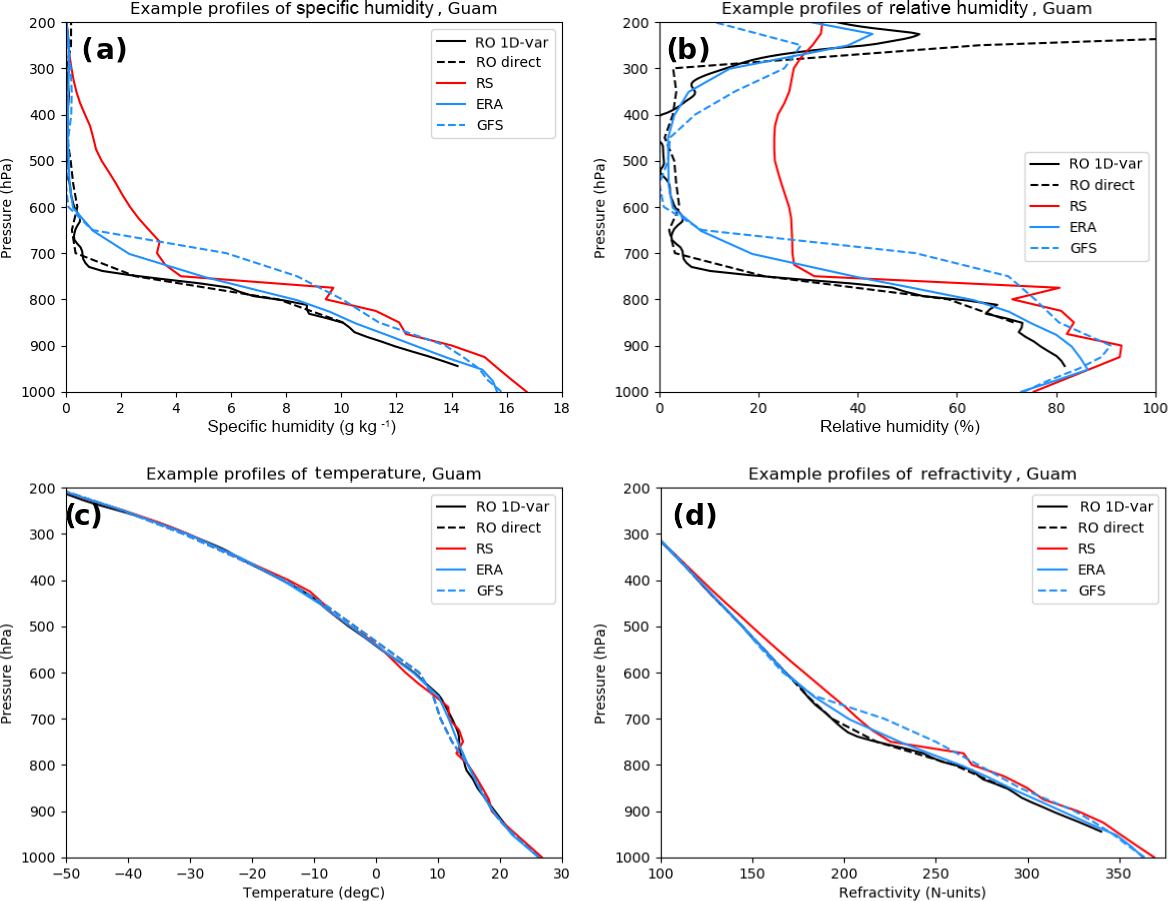
Figure 3Profiles of specific humidity (a), relative humidity (b), temperature (c), and refractivity (d) for the five data sets for 13 January 2007 at 00:23 UTC.

A comparison of Figs. 3 and 4 shows that the normalized-difference profiles highlight the similarities and differences of the five data sets better than the actual profiles, especially in the upper troposphere. The magnitudes of the normalized differences are the same order of magnitude at all levels, whereas the differences in the actual profiles can vary by more than an order of magnitude from the lower to the upper troposphere. Figure 4 shows that typical percentage differences between data sets are ∼ 50 % for q and RH, 0.5 % for T, and 5 % for N.
2.8 Representativeness errors
As in the apparent-error method, the 3CH error estimates include representatives errors. Since four of the five data sets considered here are representative of horizontal averages with a length scale of ∼ 100 km, while the RS data are point measurements, the differences between the RS and other data sets include a significant “representativeness” component (Kitchen, 1989). O'Carroll et al. (2008) discuss the importance of representativeness errors and how they relate to the concept of “truth” that is used in the 3CH method.
In this section we summarize the derivation of the equations relating the error variances and covariances among the data sets. The complete derivation and a discussion of the limitations are given in Appendix A.
The error variance of a variable X (e.g., q, RH, T, or N) is defined as
where true is the true (but unknown) value of X and the summation is over n samples.
As shown in Appendix A, we can derive three different linearly independent equations for estimating the error variance of any data set, assuming that the error covariances among all the data sets are negligible compared to the differences in the observed mean square (MS) differences between the data sets. The three complete (and exact) linearly independent solutions for estimating the error variance of RO are
where RO (or ERA, GFS, RS) corresponds to the value of X as estimated by RO (or ERA, GFS, RS) and MS denotes the mean square difference between the values from two data sets (e.g., RO–ERA).
We use Eqs. (7)–(9) to provide three independent estimates of VARerr(RO) by neglecting the COVerr terms in each equation. The assumption that the error covariances are small compared to the difference in variances between the data sets is similar to the assumption used in the apparent-error method that the errors of the observations and model forecasts are uncorrelated. In general the COVerr terms are not zero; thus we will examine the validity of this assumption by checking whether the various estimates of the error variances from the three equations are consistent with each other and reasonable compared to other independent studies that estimate error variances in other ways. In a related paper (Rieckh and Anthes, 2018) we examine the effect of various degrees of error correlations between two of the three data sets using simulated data sets with known errors.
The same procedure can be used to derive three equations for estimating the error variances for the other three data sets, RS, ERA, and GFS (equations not shown here).
So for each of the five data sets – RO-direct and RO 1D-VAR, RS, ERA, and GFS – there are three independent ways to estimate their respective error variances. This is the three-cornered hat method described in Appendix A. We note that it is possible that the estimated error variances from any of the three equations are negative because of the neglect of the COVerr terms and the small sample size, especially above 300 hPa for the Japanese stations and below 800 hPa for all four stations (Fig. 1).
We first compute the estimated error variance for RO refractivity using GFS and ERA data for comparison with the Kuo et al. (2004) and Chen et al. (2011) estimates of RO error variance to illustrate the 3CH method. In an analogy to the apparent-error equation (Eq. 4), with RO being the observation and ERA being the forecast,
which is Eq. (A2) in Appendix A with neglect of the COVerr terms. We compute MS(RO–ERA) from the RO and ERA data sets (analogous to the apparent error variance in Eq. 4) and plot its square root as the black line in Fig. 5. Then we estimate VARerr(RO) using Eq. (7) and the data sets (RO–GFS) and (GFS–ERA), neglecting the COVerr terms.
The square root of VARerr(RO) gives the standard deviation (SD) (Fig. 5, blue curve). Finally, the ERA error variance (analogous to the forecast error) is obtained by subtracting VARerr(RO) from MS(RO–ERA) using Eq. (10) above (pink line in Fig. 5). The gap in the computed ERA error SD in Fig. 5a occurs due to negative estimated error variance values, which can result from having a limited sample size, neglecting the error covariance terms, and having an error variance that is already close to zero (as is the case for ERA).
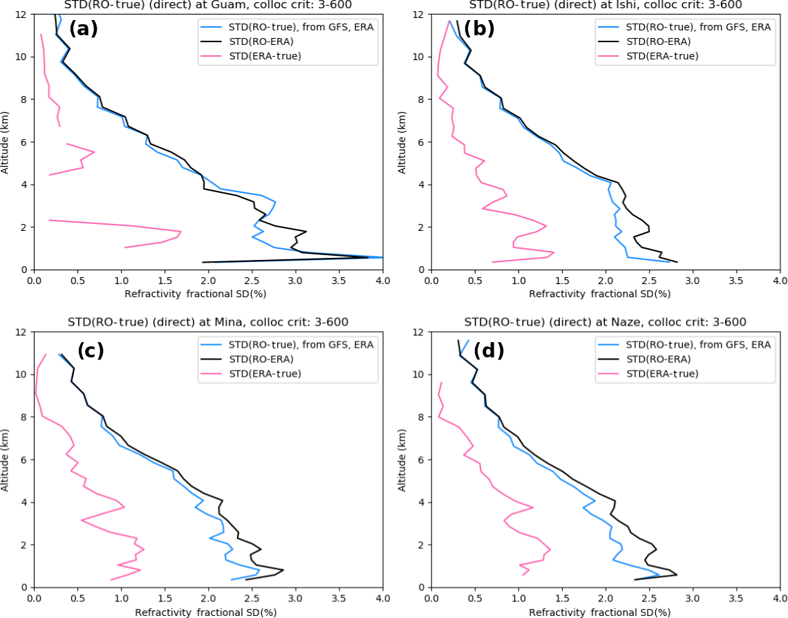
Figure 5Standard deviations of the apparent-error SD(RO–ERA) (black line), estimated RO error SD(RO–true) computed from Eq. (7) (blue line) and ERA error SD(ERA–true) (pink line) for refractivity at (a) Guam, (b) Ishi, (c) Mina, and (d) Naze.
The results shown in Fig. 5 are quite similar to those from Kuo et al. (2004) and Chen et al. (2011), who used different models and different data sets. The SD of normalized RO refractivity errors is a maximum of between 2.0 and 2.5 % near the surface, decreasing to about 0.5 % at 10 km. These similarities give credibility to both methods.
This section shows the estimated error variances for N, q, T, and RH at one of the four stations (Mina) for the five data sets and summarizes the results for the other three stations (Naze, Ishi, and Guam).
5.1 Results for Mina
The following plots show the estimated error variances computed from Eqs. (7), (8), or (9). Two RO data sets (direct and 1D-VAR) are considered one at a time using the other three data sets. Thus we have two sets of error estimates for each data set: one using the RO-direct with RS, ERA, and GFS, and one using the RO 1D-VAR with RS, ERA, and GFS. In the following plots, darker colors correspond to the three results using the RO 1D-VAR, and lighter colors correspond to the three results using the RO-direct.

Figure 6Estimated error variances (percent squared) of specific humidity at Mina: (a) RO, (b) RS, (c) GFS, and (d) ERA.

Figure 7Estimated error variances (percent squared) of relative humidity at Mina: (a) RO, (b) RS, (c) GFS, and (d) ERA.
Figure 6 shows the results for specific humidity. Error variances are shown rather than SDs because they are easier to interpret using the three equations used to derive them and because the SD are undefined for the occasional negative estimated error variance. Figure 6a shows the q error variance profiles for the two RO data sets (direct and 1D-VAR). The direct method (use of GFS temperature in Eq. 5) shows a steady increase of error variance with height, from about 100 %2 (SD ∼ 10 %) at 950 hPa to 800 %2 (SD ∼ 28 %) at 500 hPa and 2000 %2 (SD ∼ 45 %) at 300 hPa. This is expected since the refractivity contains little information on water vapor above about 400 hPa and we are using an independent estimate of temperature, with no constraints on the water vapor retrieval. The q error variance profile for RO using the 1D-VAR method is similar to that of the direct method below 500 hPa but reaches a maximum at about 500 hPa of about 500 %2 (SD ∼ 22 %) and then decreases toward zero at 200 hPa. The 1D-VAR method uses the ERA-Interim fields as a background and thus constrains the water vapor profile retrieval at high altitudes. It is notable that the three equations used to estimate the error variance profiles agree closely and the difference among the three estimates is much smaller than the differences in the mean profiles using the two RO retrieval methods.
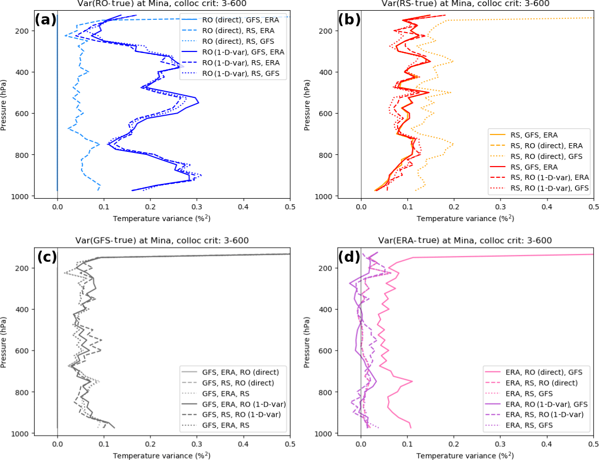
Figure 8Estimated error variances (percent squared) of temperature at Mina: (a) RO, (b) RS, (c) GFS, and (d) ERA.
The RS specific humidity error variance profiles at Mina (Fig. 6b) show a similar behavior to the RO-direct, with a steady increase with height, exceeding 2000 %2 (SD of ∼ 45 %) at 400 hPa. The SDs of the RS are slightly larger than the two RO estimates below 600 hPa. The larger error variance of RS compared to RO is consistent with the results from Kuo et al. (2004) and is due in part to the RS representativeness differences. The error variance estimates using the RO-direct (orange) and RO 1D-VAR (red) are similar.
The error variance profiles from the two model sets (Fig. 6c, d) are quite different. The GFS error variance is less than the RO-direct and RS error variances at all levels, and also less than the RO 1D-VAR error variance except above 300 hPa. Although there is more scatter, especially in the upper troposphere, the ERA profiles are different from all the other data sets in that they show only a small increase of error variance with height, from near zero at the surface to up to a mean of about 100 %2 (SD ∼ 10 %) at 200 hPa.
Figure 7 shows the estimated error variances of relative humidity. As with specific humidity, there is consistency among the estimates for the different data sets. The general behavior of the RH error variance profiles is similar to that for q, as might be expected because the percentage variability of water vapor is greater than that of temperature at this subtropical location. Again, the estimated error variances of the RO-derived RH are less than those of the RS in the lower troposphere. The GFS error variances are smaller than the RO and RS variances, except for the RO 1D-VAR profile above 300 hPa, which is constrained by the ERA observations in the upper troposphere. The ERA error variances are significantly smaller than the other data sets, averaging between 50 and 200 %2 (SD 7–14 %) throughout the troposphere.
Figure 8 shows the estimated error variances of temperature. Because the RO-direct retrieval uses the exact GFS temperature, the results for the direct retrieval (light blue) using (RO, GFS, and ERA) and (RO, RS, and GFS) are not meaningful in Fig. 8a (they are identically zero). The result from Eq. (8) (RO, ERA, and RS), given by the dashed light blue line in Fig. 8a is valid, but in reality this is an estimate of the GFS T error variance, and it is in fact very similar to the profiles in Fig. 8c.
The RO 1D-VAR results for temperature from all three equations give somewhat larger results (Fig. 8, dark blue profiles). The estimated error variance profiles oscillate between 0.1 and 0.3 %2 (SD 0.3 to 0.55 %). For a temperature of 300 K, these correspond to 0.9 to 1.65 K.
The RS temperature error variances (Fig. 8b) vary between 0.05 and 0.15 %2 (SD 0.2 to 0.4 % or 0.6 to 1.2 K for T=300 K). The GFS temperature error variances are a little lower, averaging around 0.05 to 0.10 %2 (SD 0.2 to 0.3 %), while the ERA-estimated temperature error variances average close to zero (Fig. 8d).
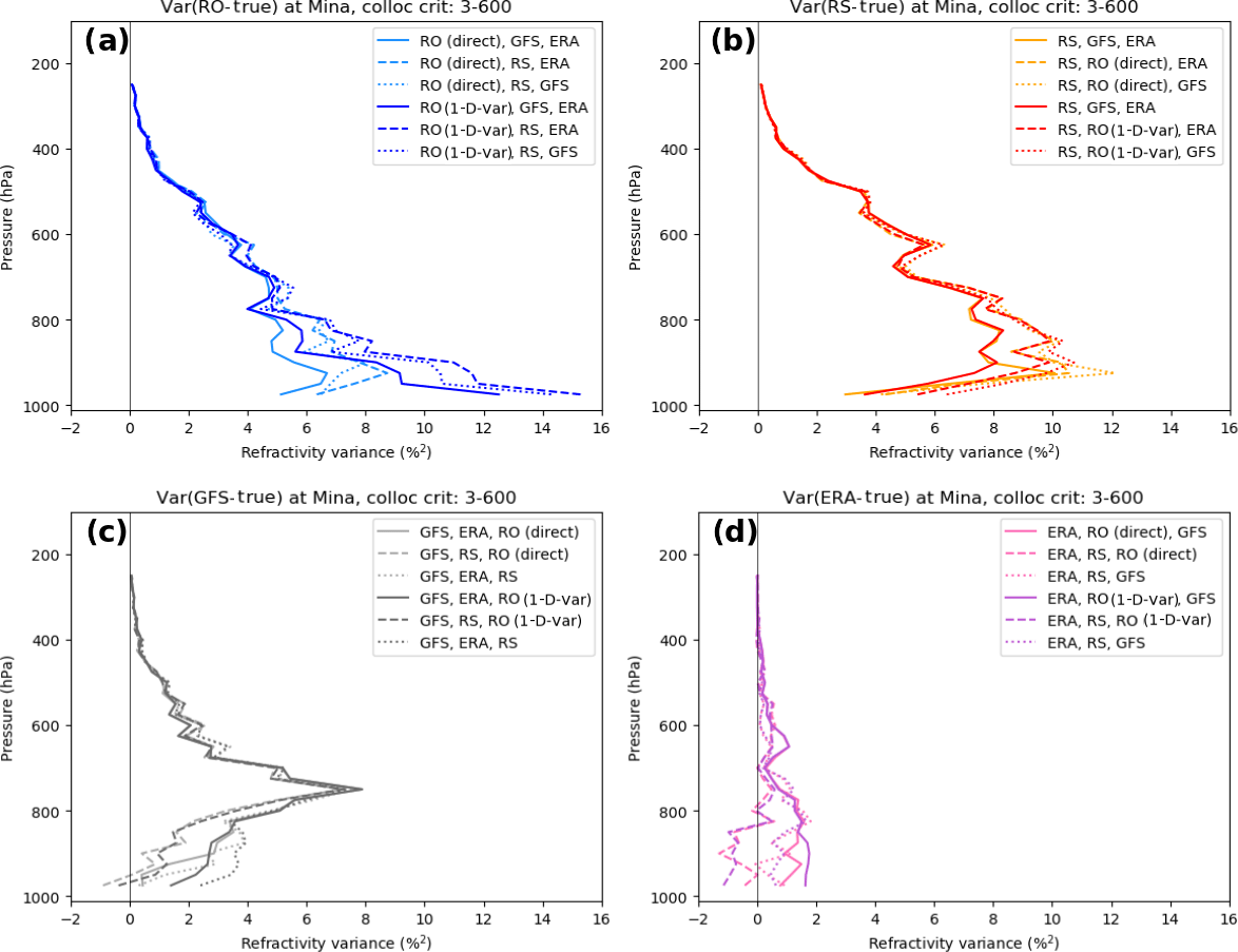
Figure 9Estimated error variances (percent squared) of refractivity at Mina: (a) RO, (b) RS, (c) GFS, and (d) ERA.
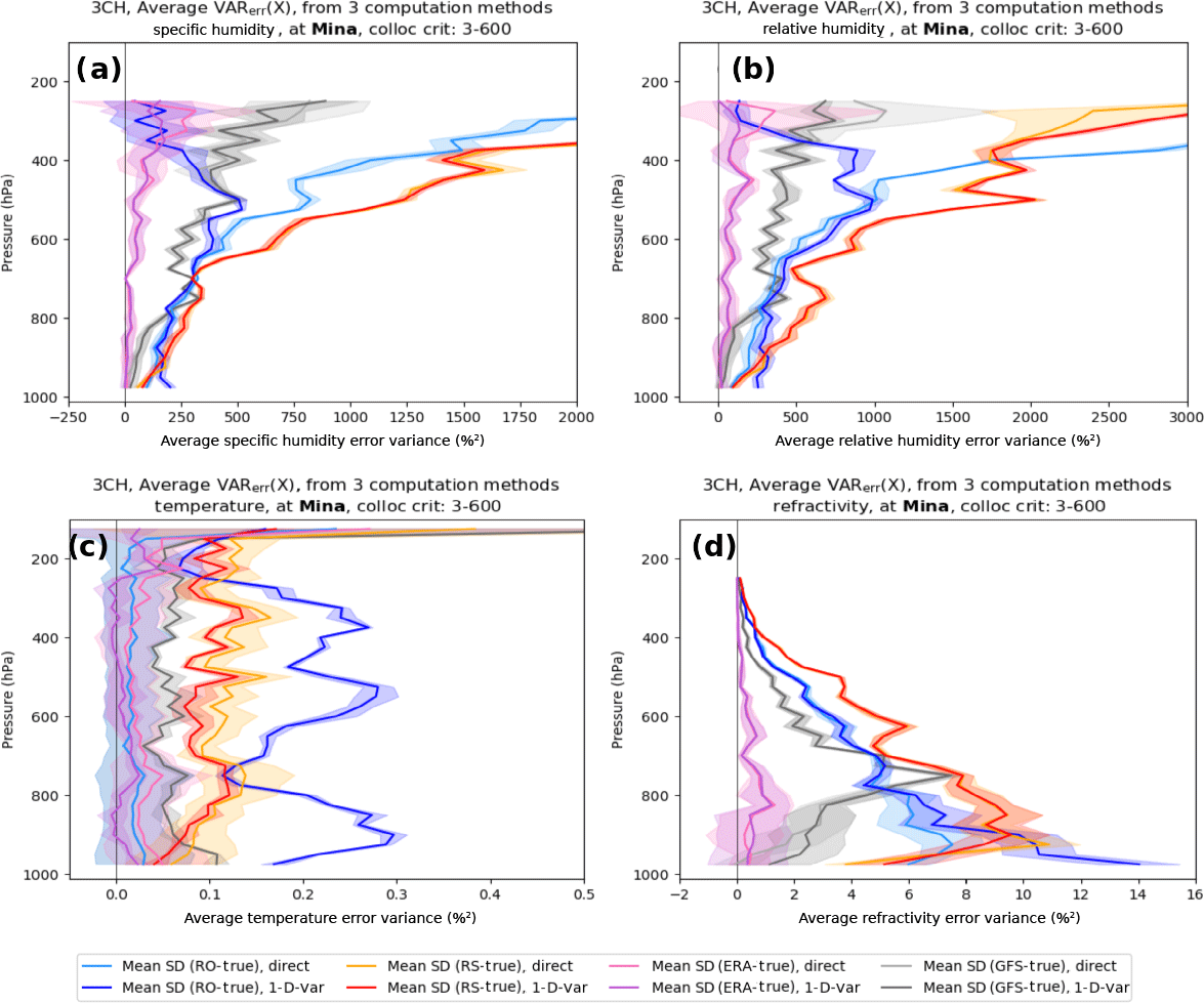
Figure 10Mean of the three estimates of error variance plots for q, RH, T, and N using RO-direct and RO 1D-VAR for each data set at Mina. The standard deviation about the mean is indicated by shaded areas. (a) specific humidity, (b) relative humidity, (c) temperature, and (d) refractivity. RO (blue), radiosonde (red), GFS (gray), and ERA (purple).
Figure 9 shows the estimates of the normalized refractivity errors for the five data sets. There is more spread in the refractivity estimates compared to those of the other variables, especially in the lower troposphere, where the estimates vary between about 4 and 9 %2 (SD 2 to 3 %) for the two RO variances. Recall that the RO-direct N are the observed RO N as provided by CDAAC, while the RO 1D-VAR N are modified based on the background (ERA) N. The average of the N error variances for the radiosondes (Fig. 9b) shows a maximum of ∼ 10 %2 (SD ∼ 3.2 %) around 900 hPa. The GFS error variance profiles show a maximum around 750 hPa of ∼ 8 %2 (SD ∼ 2.8 %). The ERA profiles show the smallest errors, with a maximum in the lower troposphere of an average of ∼ 2 %2 (SD ∼ 1.4 %). All data sets show a decrease of error variance to less than 0.5 %2 (SD < 0.7 %) at 400 hPa. The reason for the large scatter in estimates of N below about 800 hPa may be related to errors in N caused by super-refraction in the lower troposphere, which occurs often in the tropics and subtropics. Super-refraction causes a negative N bias, which may lead to larger error covariances in this layer. The smaller number of RO samples below 800 hPa (Fig. 1) may also be a factor.
Figure 10 shows the mean of the three estimates of the error variances of the five data sets for q, RH, T, and N at Mina. The standard deviation1 about these means is shown by the shaded areas. These figures show clearly the significant differences among the error variance estimates of the five data sets. In Fig. 10a, the error variance for specific humidity is greatest for the radiosonde (red and orange profiles) and least for the ERA profiles. As discussed earlier, the mean of the RO 1D-VAR retrieval reaches a maximum at about 550 hPa and then decreases back toward zero as it becomes constrained by the background profile at high levels. Figure 10b–d show the mean profiles of error variance for relative humidity, temperature, and refractivity. The relative humidity profiles are similar to the specific humidity profiles. The ERA errors are the smallest, followed by GFS, the RO, and finally the radiosondes. The temperature error variance profiles show that the ERA errors are very close to zero throughout the entire troposphere. The GFS profiles (gray) and the RS profiles (red and orange) show relatively constant values with height of approximately 0.05 and 0.1 %2, respectively (corresponding to temperature errors of 0.7 and 0.9 K at 300 K, respectively). The RO shows an oscillating error variance profile ranging between 0.1 and 0.3 %2 (0.9 and 1.6 K at 300 K). Finally, the refractivity profiles show the greatest variability, but the mean profiles are still quite distinct. ERA again shows the lowest errors, followed by GFS, RO, and RS.
It is difficult to find previous results for RS temperature and specific humidity error variances. However, previous studies comparing RO with RS and models indicate that our estimates are reasonable and consistent with these studies. Ho et al. (2017) found SD between RO and RS pairs for many RS types of about 1.5 K in the 200–20 hPa layer, where RO temperatures are most accurate (Table 2 in Ho et al., 2017). This value corresponds to the apparent error between RS and RO, which is larger than the RS error. The estimated RS temperature error variances from 200 to 100 hPa in Fig. 10c is about 0.15 %2, which corresponds to a SD of 0.39 % or 0.9 K for a mean temperature of 230 K. Ladstädter et al. (2015) compared high-quality GCOS (Global Climate Observing System) Reference Upper-Air Network (GRUAN) RS to RO globally and for a tropical station (Nauru) and subtropical station (Tateno, Japan) from 2002 to 2013. They found temperature SD of about 0.5 K for Nauru and 0.5 to 0.8 K at Tateno averaged over the layer 800 to 300 hPa. For specific humidity, they found SD between RO and RS of about 10 %, increasing to about 40 % in the upper troposphere. In our calculations for Guam and the three subtropical Japanese stations our estimates for SD of q are similar (Fig. 10a; Fig. B1 in Appendix B), ranging from about 10 % at 900 hPa to 45 % at 300 hPa.
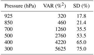
Ho et al. (2010) compared COSMIC RO observations to ECMWF analyses and several types of radiosondes for the period August–November 2006. They found mean specific humidity SD of RO–ECMWF of ∼ 0.5 g kg−1 and RO–RS (Meisei) of ∼ 0.9 g kg−1. From their plots of the vertical profiles of the SD, these numbers are typical for the layer 800–500 hPa, which, given the normalization values from the four RS stations in our study (Fig. 3) of about 9 g kg−1 at 800 hPa and 2 g kg−1 at 500 hPa, correspond to SD (VAR) values of ∼ 6 % (36 %2) at 800 hPa and 25 % (625 %2) at 500 hPa for ECMWF and ∼ 10 % (100 %2) at 800 hPa and 45 % (2025 %2) at 500 hPa for Meisei RS. These values are similar to the estimates of the RS analysis for the Japanese stations shown in Fig. B1 of Appendix B.
Vergados et al. (2014) compared RO-derived observations of specific humidity with radiosondes and ERA-Interim under cloudy conditions in the tropics for August–October 2006. They used the direct method for computing specific humidity from the RO refractivity using the ERA-Interim temperatures. Their differences between zonal means of normalized RO and ERA-Interim observations of q are presented in Table 1 (we computed the normalized differences from their data in Table 3 for the tropics).
Table 1Normalized differences of zonal mean RO and ERA specific humidity in the tropics for cloudy conditions (Vergados et al., 2014).
The VAR values in Table 1 correspond to apparent errors, where RO and ERA correspond to the observation and forecast variables, respectively (Eq. 10). As expected, they are larger than the estimated error variances for RO-direct shown in Fig. 6a because the apparent errors are always larger than the observation errors as shown in Eq. (4). This comparison indicates that the estimates of true errors in Fig. 6a are reasonable.
5.2 Summary of results at Naze, Ishi, and Guam
The mean and SD error profiles for Naze, Ishi, and Guam corresponding to the above results for Mina are presented in Appendix B. Here we summarize the main similarities and differences between the error variance estimates for these stations compared to those for Mina. In general, we find similar magnitudes and shapes of the profiles of the estimated error variances of the five data sets for all four variables (q, RH, T, and N).
The estimated error profiles are especially similar for the three Japanese stations. This close similarity may be due primarily to the fact that the three locations are relatively close together and two of the three use the same type of radiosonde (Meisei).
The results from Guam are also similar in general magnitudes and shapes of the profiles to those from the three Japanese stations, but there are somewhat greater differences in some of the profiles (e.g., GFS q, RH, and N; and RS N). These differences are likely due to the different location and the use of a different radiosonde type at Guam (VIZ/Sippican B2). The neglected error covariance terms are also likely different between the three Japanese stations, which are located in a data-rich region, and Guam, which is located in a data-sparse region. Thus the model errors are less likely to be highly correlated with a single observational system in the former than in the latter, where single observations may affect the models more significantly.
We used the three-cornered hat (3CH) method to estimate vertical profiles of error variances of different observation and model data sets by computing the differences among the data sets. We computed estimated error variances of four variables (specific humidity q, relative humidity RH, temperature T, and refractivity N) for five data sets (ERA, GFS, radiosondes (RS), and radio occultation (RO) 1D-VAR and RO-direct) at four different locations in the tropics and subtropics for the year 2007. The stations are Guam, Ishigakijima, Minamidaitōjima, and Naze. The latter three stations are on Japanese islands and are located quite close together (a few hundred kilometers apart). We computed vertical profiles of estimated error variances for normalized differences from the 2007 ERA mean values of q, RH, T, and N at the four stations using three linearly independent equations (Eqs. 7–9) neglecting all error covariance terms. Ideally, with a very large sample of data pairs and zero correlation of errors among the different data sets, all three equations would produce identical results. However, a finite data set and non-zero error correlations among the data sets lead to three different estimates, as shown by Rieckh and Anthes (2018). The differences among the three estimates is a measure of these effects.
Although the neglect of the covariance terms affects the results to a noticeable degree in some of the estimated profiles, there is strong evidence that there is valid information in the estimated error profiles that rises above the noise caused by the neglect of the covariance terms and the limited data sample. This evidence is summarized as follows:
-
There is generally good agreement in the three estimated error profiles of the four variables for each of the five data sets at all four locations. It is unlikely that this agreement would occur by chance if the neglected error covariance terms were large enough to invalidate the results, because they would have to somehow combine or cancel in each of the three equations to give the observed similar results.
-
There are large differences in the overall structure (shape and magnitude) of the average vertical profiles of estimated error variances for the five data sets (Fig. 10). These differences are significantly larger than the standard deviation from the three independent equations used to compute the error variances.
-
The variability, or spread among the error estimates, is similar at most height levels for specific humidity, relative humidity, and temperature. If the error covariance terms were significant, they would almost certainly vary with height, giving different agreement in estimated error profiles with height. For example, we know that RO temperature and refractivity are most accurate in the upper troposphere and least accurate in the lower troposphere and that the weight given to RO in the models' data assimilation varies significantly with height, being largest in the upper troposphere and smallest in the lower troposphere. Thus one would expect the RO–ERA and RO–GFS error covariance terms to vary significantly with height. Also, the RS errors as well as the ERA and GFS model errors vary with height. It is therefore unlikely that all of the neglected error covariance terms are the same at all heights.
-
The general structure and magnitudes of the estimated error variance profiles are similar at the four locations. However, there are some small differences among the profiles at the four locations. In general, the differences among the three estimates (indicated by the SD about the mean), which are a measure of the effect of the neglected covariance terms as well as limited sample size, are smallest for Ishi, Naze, and Mina and largest for Guam. Since the three Japanese stations are close together, this suggests that there is a difference in the error variance of the Japanese RS observations compared to the Guam RS observations. There may also be small differences in the model errors over the Japanese stations, which are located in a data-rich area compared to Guam, which is located in a data-sparse region. The largest variability and largest error estimates occur at Guam, which uses a radiosonde that is thought to have large water vapor biases due to sensor malfunctions (Holger Vömel, personal communication, 2017).
-
The magnitudes of the estimated RO refractivity error variances are supported by previously published studies, including Kuo et al. (2004) and Chen et al. (2011).
-
The estimated errors are smallest for the ERA-Interim model data set, which is a reasonable result since ERA uses an excellent model and data assimilation system that assimilates many independent, quality-checked observations. In fact, Vergados et al. (2015) state that “ERA-Interim is one of the most advanced global atmospheric models simulating the state of the atmosphere with accuracy similar to what is theoretically possible (Simmons and Hollingsworth, 2002) using a 4D-VAR method (Simmons et al., 2005)”.
-
Our results show, in general, that the RO observations have smaller errors than the radiosonde errors, in agreement with previous studies. This difference is in part due to representativeness errors associated with the RS, which are point measurements while the other data sets are representative of horizontal averages with a length scale of ∼ 100 km.
Code will be made available by the author upon request.
Data can be made available from authors upon request.
A1 Description of three-cornered hat method
In this appendix we summarize the 3CH method (Gray and Allan, 1974) for estimating error variances from three data sets. Gray and Allan (1974) developed the method to estimate the absolute frequency stability of an ensemble of N clocks by forming all triads under the assumption that the clock errors are uncorrelated. Each of the triads are three-cornered hat (3CH) estimates. Riley (2003) provides a summary of the 3CH method.
Variations and enhancements of the 3CH method have been applied to many diverse geophysical data sets. The 3CH method has been used to estimate the stability of GNSS clocks using the measured frequencies from multiple clocks (Ekstrom and Koppang, 2006; Griggs et al., 2014, 2015; Luna et al., 2017). Valty et al. (2013) used the 3CH method to estimate the geophysical load deformation computed from GRACE satellites, GPS vertical displacement measurements, and global general circulation models. O'Carroll et al. (2008) compared three types of systems to measure sea surface temperatures: two different radiometers and in situ observations from buoys. They discuss the assumption of the neglect of error correlations among the three data sets; the effect of representativeness errors; and the interpretation of “truth”, the true value of the variable being measured.
Closely related to the 3CH method is the triple-collocation (TC) method, which was introduced by Stoffelen (1998) and has been widely used since in oceanography and hydrometeorology (Gruber et al., 2016; Su et al., 2014). It has been used to estimate the error variances of triplets of observation types to measure a diverse set of geophysical properties, including wave heights, sea surface temperatures, precipitation, surface winds over the ocean, leaf area index (LAI) products, and soil moisture. Stoffelen (1998) estimated the error variances of in situ measurements, ERS scatterometer winds, and NCEP forecast model wind speeds. Later, Vogelzang et al. (2011) compared four sets of scatterometer winds from ASCAT and SeaWinds with buoy measurements and ECMWF model forecasts of surface winds over the oceans to estimate the error variances and standard deviations of the different data sets and their combinations. Stoffelen (1998) and Vogelzang et al. (2011) calibrate their data sets using an error model and show how the error estimates may account for a partial correlation of representativeness errors between two data sets if independent information about this correlation is known. Fang et al. (2012) estimated the uncertainties in three different estimates of LAI products. McColl et al. (2014) extended the method by deriving a performance metric of the measurement system to the unknown truth and applied the extended method to wind estimates from numerical weather prediction, scatterometer, and buoy wind estimates. Roebeling et al. (2012) used the triple-collocation method to estimate the errors associated with three ways of estimating precipitation: the Spinning Enhanced Visible and Infrared Imager (SEVERI), weather radars, and ground-based precipitation rain gauges. They concluded that the method provides useful error estimates of these systems.
The major assumption in the 3CH and TC methods is that the unknown errors of the three systems are uncorrelated. Correlations between any or all of the three measurement systems will reduce the accuracy of the error estimates. Other factors that can reduce the accuracy of the error estimates include widely different errors associated with the three systems or a small sample size. These factors can lead to negative estimates of error variances, especially when the estimates are close to zero (Gray and Allan, 1974; Riley, 2003). All three of these factors potentially affect the 3CH estimates in this paper, but the general agreement of the three linearly independent equations for estimating the error variances of each variable suggests that the estimates are still reasonably valid and contain useful information.
A2 Derivation of 3CH equations
In this section we summarize the derivation of the 3CH method as applied to four meteorological data sets, RO, RS, GFS, and ERA. The error variance of a variable X (e.g., temperature, specific humidity, relative humidity, refractivity) is defined as
where true is the true but unknown value of X and the summation is over n samples. This definition of error variance includes bias as well as random errors in X. Let RO correspond to the value of X as estimated by RO, ERA correspond to the value of X as estimated by ERA, and similarly for GFS and RS. We then have
where MS(RO–ERA) is the mean square difference between RO and ERA and the last term is the error covariance between RO and ERA.
In the estimation of the error variances for the four data sets, we assume that the RO errors and ERA errors are uncorrelated, so the error covariance term in Eq. (A2) is zero or, in practice, negligibly small compared to the other terms. However, to show the complete (and exact) equations, we retain them here in the six equations (Eqs. A2–A7) involving the different pairs of data sets.
It is possible to use these six equations to get three different, linearly independent estimates of the four unknowns error variances for RO, RS, ERA, and GFS. For RO, these three equations are
O'Carroll et al. (2008) present these equations for a system of three observation types (their Eq. 1). However, they remove the mean biases from each data set in their definition of error variance, whereas we do not in our definition (Eq. A1). Our expressions for estimated error variances are identical to those of O'Carroll et al. (2008) with the removal of the effect of these biases; e.g., replace MS(X−Y) in Eqs. (A8)–(A10) with MS(X−Y) − [M(X−Y)]2, where X and Y are any of the data sets. Removing these biases will generally result in smaller estimated error variances than the results presented in this paper.
As noted by an anonymous reviewer, it is possible to derive infinitely many linearly dependent equations by combining Eqs. (A8)–(A10) in different ways by forming combinations of the form M1× Eq. (A8) Eq. (A9) + M3× Eq. (A10), where M1, M2, and M3 are any numbers except those for which . We did not pursue this possibility in this paper but instead used the three linearly independent equations only in our estimates of error variances.
If all the neglected COVerr terms were in fact identically zero and the sample size was very large (much larger than our sample size), all three estimates of the error variances would be the same. The fact that they give different solutions is because the neglected COVerr terms are in reality not zero, and hence their neglect affects the three approximate equations in different ways to give three different solutions. The relatively small sample size n also contributes to the differences in the three solutions, which are a measure of these effects.
We also note that the error estimates contain any representativeness errors caused by the different data sets representing different scales of atmospheric structure (O'Carroll et al., 2008). Representativeness errors can occur because of different horizontal or vertical resolutions or footprints of the data sets.
A3 Brief comparison of 3CH method and TC method
While it is not the intent of this paper to do a thorough comparison of the 3CH and TC methods, which are introduced above, in response to a reviewer's comment we compared the two methods on a subset of our data sets. A difference between the 3CH and TC method is that the TC method corrects for additive and multiplicative biases among the three data sets, as discussed by Stoffelen (1998), Vogelzang et al. (2011), and others. The TC method calibrates two of the data sets against the third, eliminating biases among the three data sets. This calibration uses an error model of the form , where a and b stand for the “trend” and “bias” calibration coefficients and ei are random errors (Vogelzang et al., 2011). As shown below, calibrating our data sets according to this model gave results very similar to results using our uncalibrated data sets.
In our application of the TC method we use the following combinations of data sets: (ERA, RO, RS), (ERA, RO, GFS), and (ERA, GFS, RS). For the RO we use two RO retrievals, the direct and 1D-VAR (see Sect. 2.3). The RO, RS, and GFS data sets are all calibrated using ERA as the calibration reference, using the following calibration factors. For example, the calibrated RO and RS (designated by ROcal and RScal, respectively) using ERA as the reference are (following Stoffelen, 1998; Vogelzang et al., 2011; and Roebeling et al., 2012)
where the additive bias terms are
the multiplicative bias terms are
and M denotes the mean value over the data sets.
The results of the specific humidity error variance estimates for ROcal and RScal compared to RO and RS are shown in Fig. A1, and the estimates for ERAcal and GFScal compared to ERA and GFS are shown in Fig. A2. The left panels show the results from the TC method (calibrated data), and the right panels show the results using the 3CH method (uncalibrated data). The close similarity of the results indicates that the biases do not significantly affect the 3CH estimates, in agreement with the results from the error model study in Rieckh and Anthes (2018).

Figure A1Estimated RO and RS error variances for specific humidity at Minamidaitōjima (Japan) using calibrated data as in the TC method (a, c) and the uncalibrated data as in the 3CH method (b, d). For the TC method, the RO, RS, and GFS data sets are calibrated with respect to ERA as the reference data set. The following combinations of the four data sets are used: (ERA, RO, RS), (ERA, RO, GFS), and (ERA, GFS, RS).
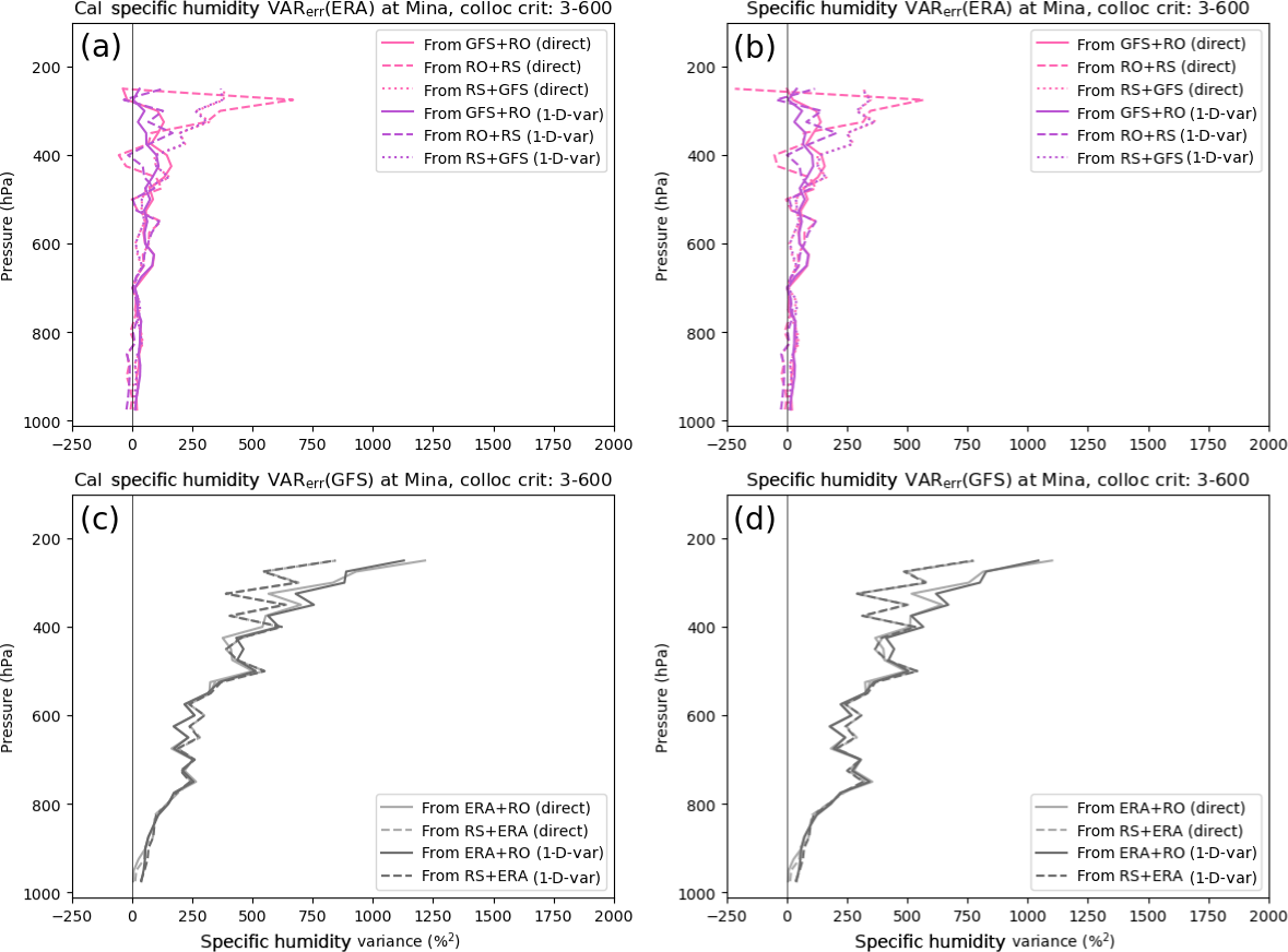
Figure A2Estimated ERA and GFS specific error variances for ERA at Minamidaitōjima (Japan) using calibrated data as in the TC method (a, c) and the uncalibrated data as in 3CH method (b, d). For the TC method, the RO, RS, and GFS data sets are calibrated with respect to ERA. The following combinations of the four data sets are used: (ERA, RO, RS), (ERA, RO, GFS), and (ERA, GFS, RS).
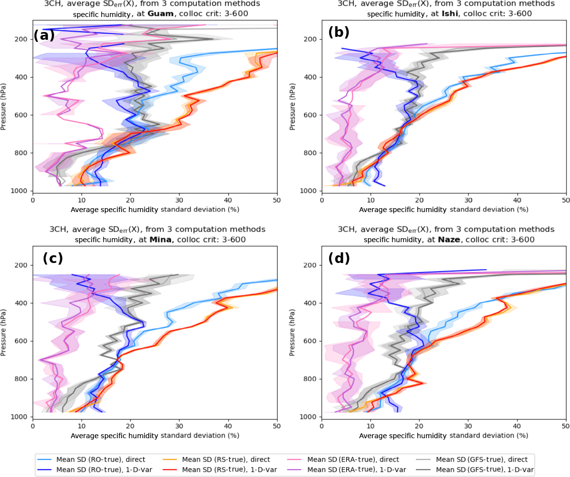
Figure B1Mean and standard deviations (shading) of the three estimates of normalized specific humidity using RO-direct and RO 1D-VAR at (a) Guam, (b) Ishi, (c) Mina, and (d) Naze.
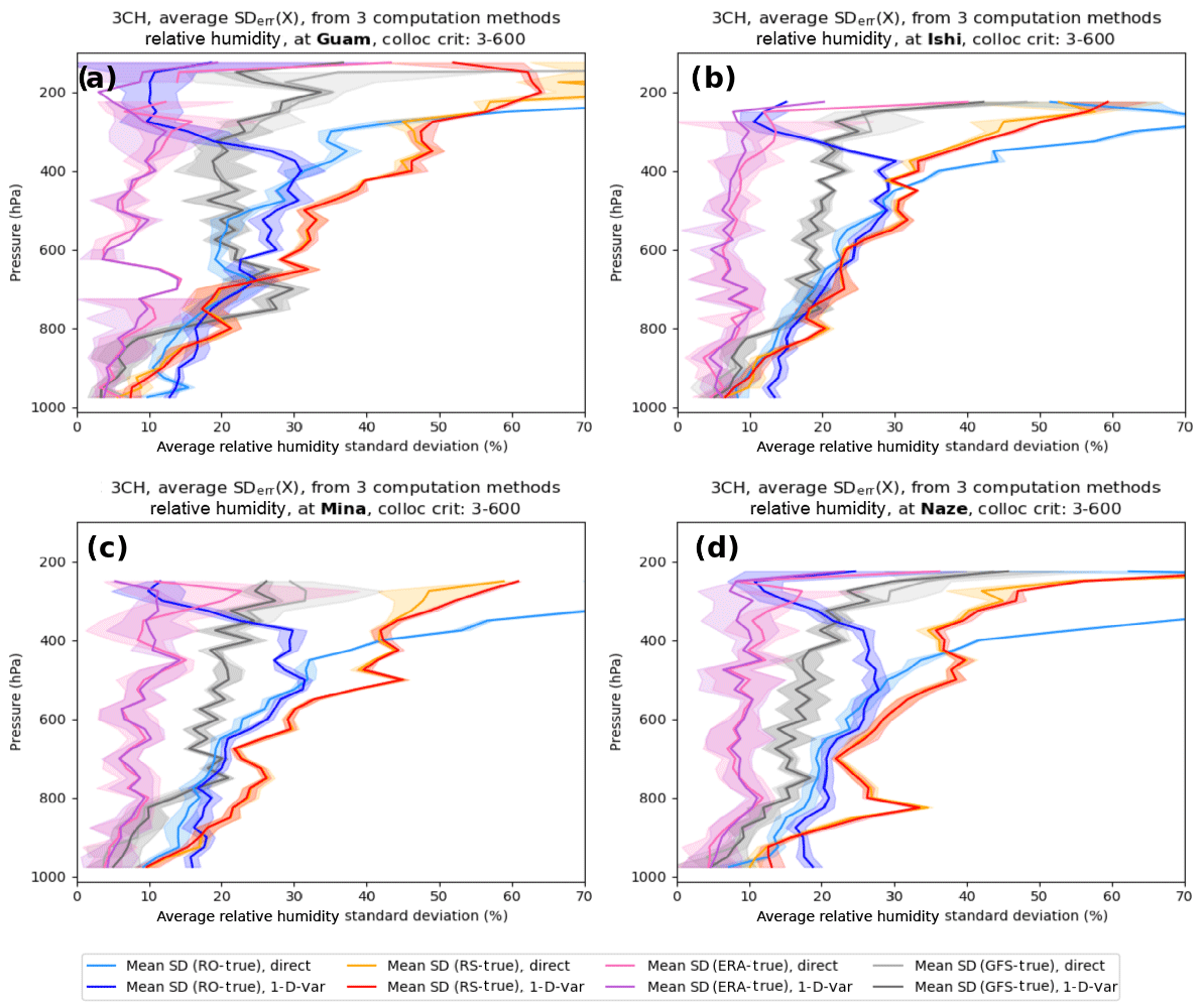
Figure B2Mean and standard deviations (shading) of the three estimates of normalized relative humidity using RO-direct and RO 1D-VAR at (a) Guam, (b) Ishi, (c) Mina, and (d) Naze.
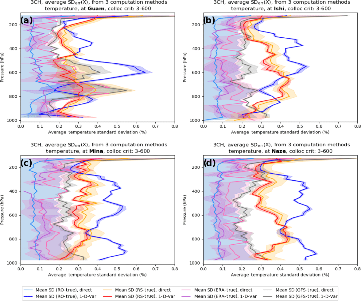
Figure B3Mean and standard deviations (shading) of the three estimates of normalized temperature using RO-direct and RO 1D-VAR at (a) Guam, (b) Ishi, (c) Mina, and (d) Naze.

Figure B4Mean and standard deviations (shading) of the three estimates of normalized refractivity using RO-direct and RO 1D-VAR at (a) Guam, (b) Ishi, (c) Mina, and (d) Naze.
RA formulated the overall idea of this work, and TR performed all the calculations and contributed significantly to the discussion of the results.
The authors declare that they have no conflict of interest.
We acknowledge with thanks the insightful comments and advice on this study
from Ian Culverwell and John Eyre (Met Office), Shay Gilpin (UCAR COSMIC), Sean Healy
(ECMWF), Adrian Simmons (ECMWF), and Sergey Sokolovskiy (UCAR COSMIC). We
thank the three anonymous reviewers for their constructive comments. Anthes
and Rieckh were supported by NSF-NASA grant AGS-1522830. We thank Eric
DeWeaver (NSF) and Jack Kaye (NASA) for their long-term support of
COSMIC.
Edited by: Ad Stoffelen
Reviewed by: three anonymous referees
Chen, S.-Y., Huang, C.-Y., Kuo, Y.-H., and Sokolovskiy, S.: Observational Error Estimation of FORMOSAT-3/COSMIC GPS Radio Occultation Data, Mon. Weather Rev., 139, 853–865, https://doi.org/10.1175/2010MWR3260.1, 2011. a, b, c, d, e, f, g
Cucurull, L. and Derber, J. C.: Operational Implementation of COSMIC Observations into NCEP's Global Data Assimilation System, Weather Forecast., 23, 702–711, https://doi.org/10.1175/2008WAF2007070.1, 2008. a
Dee, D. P., Uppala, S. M., Simmons, A. J., Berrisford, P., Poli, P., Kobayashi, S., Andrae, U., Balmaseda, M. A., Balsamo, G., Bauer, P., Bechtold, P., Beljaars, A. C. M., van de Berg, L., Bidlot, J., Bormann, N., Delsol, C., Dragani, R., Fuentes, M., Geer, A. J., Haimberger, L., Healy, S. B., Hersbach, H., Hólm, E. V., Isaksen, L., Kållberg, P., Köhler, M., Matricardi, M., McNally, A. P., Monge-Sanz, B. M., Morcrette, J.-J., Park, B.-K., Peubey, C., de Rosnay, P., Tavolato, C., Thépaut, J.-N., and Vitart, F.: The ERA-Interim reanalysis: configuration and performance of the data assimilation system, Q. J. Roy. Meteor. Soc., 137, 553–597, https://doi.org/10.1002/qj.828, 2011. a
Desroziers, G. and Ivanov, S.: Diagnosing and adaptive tuning of observation-error parameters in a variational assimilation, Q. J. Roy. Meteor. Soc., 127, 1433–1452, https://doi.org/10.1002/qj.49712757417, 2001. a
Ekstrom, C. R. and Koppang, P. A.: Error Bars for Three-Cornered Hats, IEEE T. Ultrason. Ferr., 53, 876–879, https://doi.org/10.1109/TUFFC.2006.1632679, 2006. a
ERA-Interim, available at: https://www.ecmwf.int/en/research/climate-reanalysis/reanalysis-datasets/era-interim, last access: 1 July 2018.
Fang, H., Wei, S., Jiang, C., and Scipal, K.: Theoretical uncertainty analysis of global MODIS, CYCLOPES, and GLOBCARBON LAI products using a triple collocation method, Remote Sens. Environ., 124, 610–621, https://doi.org/10.1016/j.rse.2012.06.013, 2012. a
Gilpin, S., Rieckh, T., and Anthes, R.: Reducing representativeness and sampling errors in radio occultation–radiosonde comparisons, Atmos. Meas. Tech., 11, 2567–2582, https://doi.org/10.5194/amt-11-2567-2018, 2018. a
Gray, J. E. and Allan, D. W.: A method for estimating the frequency stability of an individual oscillator, in: 28th Annual Symposium on Frequency Control, Atlantic City, New Jersey, 29–31 May 1974, IEEE, 243–246, https://doi.org/10.1109/FREQ.1974.200027, 1974. a, b, c, d
Griggs, E., Kursinski, E., and Akos, D.: An investigation of GNSS atomic clock behaviour at short time intervals, GPS Solut., 18, 443–452, https://doi.org/10.1007/s10291-013-0343-7, 2014. a
Griggs, E., Kursinski, E., and Akos, D.: Short-term GNSS satellite clock stability, Radio Sci., 50, 813–826, https://doi.org/10.1002/2015RS005667, 2015. a
Gruber, A., Su, C.-H., Zwieback, S., Crow, W., Dorigo, W., and Wagner, W.: Recent advances in (soil moisture) triple collocation analysis, Int. J. Appl. Earth Obs., 45, 200–211, https://doi.org/10.1016/j.jag.2015.09.002, 2016. a
Ho, S.-P., Zhou, X., Kuo, Y.-H., Hunt, D., and Wang, J.-H.: Global evaluation of radiosonde water vapor systematic biases using GPS radio occultation from COSMIC and ECMWF analysis, Remote Sens., 2, 1320–1330, https://doi.org/10.3390/RS2051320, 2010. a
Ho, S.-P., Peng, L., and Vömel, H.: Characterization of the long-term radiosonde temperature biases in the upper troposphere and lower stratosphere using COSMIC and Metop-A/GRAS data from 2006 to 2014, Atmos. Chem. Phys., 17, 4493-4511, https://doi.org/10.5194/acp-17-4493-2017, 2017. a, b
Hollingsworth, A. and Lönnberg, P.: The statistical structure of short-range forecast errors as determined from radiosonde data. Part I: The wind field, Tellus A, 38, 111–136, https://doi.org/10.3402/tellusa.v38i2.11707, 1986. a
Kitchen, M.: Representativeness errors for radiosonde observations, Q. J. Roy. Meteor. Soc., 115, 673–700, https://doi.org/10.1002/qj.49711548713, 1989. a
Kleist, D. T., Parrish, D. F., Derber, J. C., Treadon, R., Wu, W.-S., and Lord, S.: Introduction of the GSI into the NCEP Global Data Assimilation System, Weather Forecast., 24, 1691–1705, https://doi.org/10.1175/2009WAF2222201.1, 2009. a
Kuo, Y.-H., Wee, T.-K., Sokolovskiy, S., Rocken, C., Schreiner, W., Hunt, D., and Anthes, R. A.: Inversion and error estimation of GPS radio occultation data, J. Meteorol. Soc. Jpn., 82, 507–531, 2004. a, b, c, d, e, f, g
Ladstädter, F., Steiner, A. K., Schwärz, M., and Kirchengast, G.: Climate intercomparison of GPS radio occultation, RS90/92 radiosondes and GRUAN from 2002 to 2013, Atmos. Meas. Tech., 8, 1819–1834, https://doi.org/10.5194/amt-8-1819-2015, 2015. a
Luna, D., Pérez, D., Cifuentes, A., and Gómez, D.: Three-Cornered Hat Method via GPS Common-View Comparisons, IEEE T. Instrum. Meas., 66, 2143–2147, https://doi.org/10.1109/TIM.2017.2684918, 2017. a
McColl, K., Vogelzang, J., Konings, A., Entekhabi, D., Piles, M., and Stoffelen, A.: Extended triple collocation: Estimating errors and correlation coefficients with respect to an unknown target, Geophys. Res. Lett., 41, 6229–6236, https://doi.org/10.1002/2014GL061322, 2014. a
O'Carroll, A. G., Eyre, J. R., and Saunders, R. S.: Three-way error analysis between AATSR, AMSR-E, and in situ sea surface temperature observations, J. Atmos. Ocean. Tech., 25, 1197–1207, https://doi.org/10.1175/2007JTECHO542.1, 2008. a, b, c, d
Parrish, D. F. and Derber, J. C.: The National Meteorological Center's Spectral Statistical-Interpolation analysis system, Mon. Weather Rev., 120, 1747–1763, https://doi.org/10.1175/1520-0493(1992)120<1747:TNMCSS>2.0.CO;2, 1992. a
Rieckh, T. and Anthes, R.: Evaluating two methods of estimating error variances using simulated data sets with known errors, Atmos. Meas. Tech. Discuss., https://doi.org/10.5194/amt-2018-75, in review, 2018. a, b, c
Rieckh, T., Anthes, R., Randel, W., Ho, S.-P., and Foelsche, U.: Evaluating tropospheric humidity from GPS radio occultation, radiosonde, and AIRS from high-resolution time series, Atmos. Meas. Tech., 11, 3091–3109, https://doi.org/10.5194/amt-11-3091-2018, 2018. a, b
Riley, W. J.: Application of the 3-cornered hat method to the analysis of frequency stability, Hamilton Technical Services, available at: http://www.wriley.com/3-CornHat.htm (last access: 1 July 2018), 2003. a, b
Roebeling, R. A., Wolters, E. L. A., Meirink, J. F., and Leijnse, H.: Triple collocation of summer precipitation retrievals from SEVIRI over Europe with gridded rain gauge and weather radar data, J. Hydrometeorol., 13, 1552–1566, https://doi.org/10.1175/JHM-D-11-089.1, 2012. a, b
Simmons, A. J. and Hollingsworth, A.: Some aspects of the improvement in skill of numerical prediction, Q. J. Roy. Meteor. Soc., 128, 647–677, https://doi.org/10.1256/003590002321042135, 2002. a
Simmons, A. J., Hortal, M., Kelly, G., McNally, A., Untch, A., and Uppala, S.: ECMWF Analyses and Forecasts of Stratospheric Winter Polar Vortex Breakup: September 2002 in the Southern Hemisphere and Related Events, J. Atmos. Sci., 62, 668–689, https://doi.org/10.1175/JAS-3322.1, 2005. a
Smith, E. and Weintraub, S.: The constants in the equation for atmospheric refractive index at radio frequencies, Proc. IRE, 41, 1035–1037, 1953. a
Stoffelen, A.: Toward the true near-surface wind speed: Error modeling and calibration using triple collocation, J. Geophys. Res., 103, 7755–7766, https://doi.org/10.1029/97JC03180, 1998. a, b, c, d, e, f
Su, C.-H., Ryu, D., Crow, W. T., and Western, A. W.: Beyond triple collocation: Applications to soil moisture monitoring, J. Geophys. Res., 119, 6419–6439, https://doi.org/10.1002/2013JD021043, 2014. a
Valty, P., de Viron, O., Panet, I., Camp, M. V., and Legrand, J.: Assessing the precision in loading estimates by geodetic techniques in Southern Europe, Geophys. J. Int., 194, 1441–1454, https://doi.org/10.1093/gji/ggt173, 2013. a
Vergados, P., Mannucci, A. J., and Ao, C. O.: Assessing the performance of GPS radio occultation measurements in retrieving tropospheric humidity in cloudiness: A comparison study with radiosondes, ERA-Interim, and AIRS data sets, J. Geophys. Res.-Atmos., 119, 7718–7731, https://doi.org/10.1002/2013JD021398, 2014. a, b
Vergados, P., Mannucci, A. J., Ao, C. O., Jiang, J. H., and Su, H.: On the comparisons of tropical relative humidity in the lower and middle troposphere among COSMIC radio occultations and MERRA and ECMWF data sets, Atmos. Meas. Tech., 8, 1789–1797, https://doi.org/10.5194/amt-8-1789-2015, 2015. a
Vogelzang, J., Stoffelen, A., Verhoef, A., and Figa-Saldaña, J.: On the quality of high-resolution scatterometer winds, J. Geophys. Res., 116, C10033, https://doi.org/10.1029/2010JC006640, 2011. a, b, c, d, e
, where xn denote the three error variance estimates.
- Abstract
- Introduction
- Discussion of data sets
- Derivation of error variances
- Comparison with previous studies for RO refractivity
- Calculation of the error variance terms using multiple data sets
- Summary and discussion
- Code availability
- Data availability
- Appendix A: Derivation of estimates of error variances using four data sets and the three-cornered hat method
- Mean and standard deviations of three independent error estimates of q, RH, T, and N using RO-direct and RO 1D-VAR at Guam, Ishi, Mina and Naze
- Author contributions
- Competing interests
- Acknowledgements
- References