the Creative Commons Attribution 4.0 License.
the Creative Commons Attribution 4.0 License.
 | 20 Jul 2018
Evaluating two methods of estimating error variances using simulated data sets with known errors
Therese Rieckh
In this paper we compare two different methods of estimating the error variances of two or more independent data sets. One method, called the “three-cornered hat” (3CH) method, requires three data sets. Another method, which we call the “two-cornered hat” (2CH) method, requires only two data sets. Both methods have been used in previous studies to estimate the error variances associated with a number of physical and geophysical data sets. A key assumption in both methods is that the errors of the data sets are not correlated, although some studies have considered the effect of the partial correlation of representativeness errors in two or more of the data sets.
We compare the 3CH and 2CH methods using a simple model to simulate three and two data sets with various error correlations and biases. With this model, we know the exact error variances and covariances, which we use to assess the accuracy of the 3CH and 2CH estimates. We examine the sensitivity of the estimated error variances to the degree of error correlation between two of the data sets as well as the sample size. We find that the 3CH method is less sensitive to these factors than the 2CH method and hence is more accurate. We also find that biases in one of the data sets has a minimal effect on the 3CH method, but can produce large errors in the 2CH method.
- Article
(3023 KB) - Full-text XML
- BibTeX
- EndNote


In atmospheric sciences, observations and models are often combined with the goal of providing accurate and complete representations of the current or future state of the atmosphere. Knowing the error characteristics of observations and models is important to understanding the degree to which atmospheric phenomena of interest are accurately described and analyzed. Estimating observational and modeling error characteristics is thus of inherent scientific interest. In addition, knowing the error characteristics is important for practical applications such as data assimilation and numerical weather prediction. In many modern data assimilation schemes, observations of a given type are weighted proportionally to the inverse of their error variance (e.g., Desroziers and Ivanov, 2001).
There are several somewhat similar methods for estimating the error variances associated with two or more data sets. The “three-cornered hat” (3CH) method and the closely related “triple collocation” (TC) method have been used in physics, oceanography and other scientific disciplines to estimate the errors associated with three independent data sets. Braun et al. (2001) combined two independent data sets, Global Positioning System (GPS) slant water vapor (SWV) and water vapor radiometer (WVR), to estimate the SWV and WVR errors. In analogy to the 3CH method, we refer to the Braun et al. (2001) method as the “two-cornered hat” (2CH) method. Kuo et al. (2004) and Chen et al. (2011) used the “apparent error” (AE) method, which is a variation of the 2CH method, to estimate the error of radio occultation (RO) observations using the known (or estimated) error variance of a forecast model.
The 3CH method was originally developed as the “N-cornered hat” method (Gray and Allan, 1974) for estimating error variances from N atomic clocks. Requiring three data sets at a minimum, the 3CH method produces estimates of the error variances of each of three data sets. Riley (2003), and references therein, provide a summary of the 3CH method. Variations and enhancements of the method have been applied to many diverse geophysical data sets. The 3CH method has been used to estimate the stability of GNSS clocks using the measured frequencies from multiple clocks (Ekstrom and Koppang, 2006; Griggs et al., 2014, 2015; Luna et al., 2017). Valty et al. (2013) used the 3CH method to estimate the geophysical load deformation computed from GRACE satellites, GPS vertical displacement measurements, and global general circulation models. O'Carroll et al. (2008) compared three systems to measure sea surface temperatures: two different radiometers and in situ observations from buoys. They discuss the assumption of neglecting the error correlations among the three data sets and the effect of representativeness errors. Anthes and Rieckh (2018) used the 3CH method to estimate the error variances of three observational (two radio occultation retrievals and radiosondes) and two model data sets using various combinations of the five data sets.
The major assumption in all of the above methods is that the errors of the three systems are uncorrelated. Correlations between any or all of the three measurement systems will reduce the accuracy of the error estimates. Other factors that can reduce the accuracy include widely different errors associated with the three systems or a small sample size. These factors can lead to negative estimates of error variances, especially when the estimates are close to zero (Gray and Allan, 1974; Riley, 2003; Griggs et al., 2014).
Stoffelen (1998) developed a closely related method, termed the TC method, to estimate both errors and linear calibration coefficients of surface winds using three data sets. Stoffelen (1998) discussed the correlation between part of the representativeness errors of two of the data sets and subtracted the variance common to the scale of these errors from the estimated error variance of one of the data sets used in his pairwise estimate of error variances. This correction requires an independent estimate of the correlated part of the representativeness error. All variations of TC methods assume that, apart from the correlated part of the representativeness errors, the errors of the different observation systems are uncorrelated.
Variations of Stoffelen's TC method have been have been widely used in the fields of oceanography and hydrometeorology (e.g., Su et al., 2014; Gruber et al., 2016). Roebeling et al. (2012) used the TC method to estimate the errors associated with three ways of measuring precipitation: the Spinning Enhanced Visible and Infrared Imager (SEVIRI), weather radars and ground-based rain gauges.
In this paper we estimate the effect of neglecting the error covariances using two or three simulated data sets for which the true error variances and covariances are known. We develop a model to simulate the data sets with random and bias errors using a set of assumed true profiles. We then calculate the true error variance and covariance terms in the simulated data sets and show the impact of neglecting these terms on the estimated error variances.
We assume we have three data sets, X, Y and Z, that are all measuring the same physical variable, e.g., specific humidity, q, at the same location and time.
The error variance of the data set X is defined as
where true is the true (but unknown) value of X (as well as Y and Z), Xerr = (X − true), and n is the number of samples. As discussed in Anthes and Rieckh (2018), this definition includes bias as well as random errors in X. O'Carroll et al. (2008) provide an excellent discussion of the meaning of “true” in the context of the 3CH method.
The error covariance of the data sets X and Y is defined as
In general, the errors of X, Y and Z may be correlated or not.
2.1 Three-cornered hat method
In the 3CH method, the relationship between the error variances, the mean square (MS) differences of X and Y (MS(X−Y)), and their error covariances are given by Eqs. (7)–(9) of Anthes and Rieckh (2018):
The last three covariance terms in Eqs. (3)–(5) are unknown for real data sets, unless they are estimated independently, and are neglected when estimating the error variances of the real data sets X, Y and Z. This assumption is valid for no correlation between the errors of the data sets and a large sample size. The estimated error variances are therefore
2.2 Two-cornered hat method
The 2CH method uses only two data sets, X and Z. The derivation is presented in Appendix A. The 2CH method error variances for X and Z are given as
and
where M(X) is the mean value of X. The last three error terms in Eqs. (6) and (7) are unknown for real data sets, unless they are estimated independently, and are neglected when estimating the error variances of the real data sets X and Z:
Equations (6a) and (7a) are equivalent to Eqs. (12) and (13) of Braun et al. (2001).
An alternative form of Eqs. (6a) and (7a) that is used in some studies (e.g., Stoffelen, 1998; Vogelzang et al., 2011) is
2.3 Comparison of neglected terms in 3CH and 2CH methods
In the 3CH method, the neglected error terms when computing VARerr(X) with Eq. (3) are COVerr(X,Y) + COVerr(X,Z) − COVerr(Y,Z).
In the 2CH method, the neglected error terms when computing VARerr with Eq. (6) are −2 M(true, Xerr) + COVerr(X,Z) + M(true, Xerr + Zerr).
We note that the neglected error terms in the 2CH method contain terms involving the product of true with errors, unlike in the 3CH method. Because true is typically an order of magnitude greater than the errors, these terms are likely much larger than the neglected terms involving only products of errors, as in the 3CH method. We also note that if the errors are random and uncorrelated, all of the error terms will be zero for an infinite sample size. However, for finite sample sizes, these terms will be non-zero even if these conditions are met.
2.4 Side note: apparent error method
We note that Eq. (A6) in Appendix A is the basis for the AE method in which X is an observed data set (Xobs) and Z is a forecast of the X data set (Xfcst)
The AE is equivalent to the observation minus background (O − B) statistic used in data assimilation studies. In the AE method, the correlation of errors between the observations and forecasts is assumed negligible and the error variance of the forecast is obtained from an independent estimate.
We first generate a set of n vertical profiles of a variable, true, which we take as specific humidity from the ERA-Interim reanalysis (ERA) (Dee et al., 2011), normalized by the mean specific humidity averaged over all samples. We next generate three data sets X, Y and Z that are approximations of true (true plus random errors), where the errors of X and Z are correlated to a degree that we can control. For simplicity, we assume the errors for Y are always uncorrelated with those of X and Z. This is analogous to a system of three observational systems in which the errors of two of them are correlated, but the errors of the third are not. In this section, only random errors are considered. The effect of bias errors is discussed in Sect. 4.4.2.
We then look at the magnitude of the error terms in the 2CH and 3CH methods with various assumed correlation coefficients between the errors in X and Z and compare the estimated error variances of X, Y and Z with their true error variances. Our tests will show the impact of the neglect of the error terms depending on the degree of error correlation between X and Z.
The assumed normalized random error model for X is given by
where random [−1.7, 1.7] is a random number between −1.7 and 1.7, and the standard deviation SD increases linearly with decreasing pressure p from a value of 0.1 (10 %) at 1000 hPa to a value of 0.436 (43.6 %) at 200 hPa. In the estimated error calculations below, the normalized Xerr is expressed as a % error and the variance is expressed as %2.
The error model is created based on error estimates of specific humidity from several studies (e.g., Kursinski et al., 1997; Collard and Healy, 2003; von Engeln and Nedoluha, 2005; Wang et al., 2013). For example, Collard and Healy (2003) found that, for tropical conditions, the percentage errors for RO specific humidity varied from approximately 10 % near the surface to about 70 % near 300 hPa. Other studies show the errors varying from about 10 % near the surface to 100 % in the upper troposphere (about 200 hPa). In our error model, we specified the SD to roughly approximate the SD of RO or radiosonde (RS) data at Minamidaitōjima (hereafter Mina), Japan (Anthes and Rieckh, 2018; Rieckh et al., 2018). The assumed SD of normalized q (percent error) given by Eq. (9) is consistent with the above empirical error estimates. Thus the error model is a reasonable one in terms of its magnitude and increase with height. Since it is intended to show the sensitivity of the 3CH and 2CH methods to varying degrees of correlation between two of the data sets used in the comparison, it is not necessary that the error model be a close replication of any particular observing system, just that the magnitude of the assumed errors and their vertical distribution be reasonable.
3.1 Calculation of correlated errors
In the calculation of the correlated errors, we first generate the random error profiles Xerr, Yerr and Qerr. All of these error profiles are uncorrelated. In general all three error profiles Xerr, Yerr and Qerr may have different standard deviations, but for these tests we assume all standard deviations vary according to Eq. (9) for simplicity. We now generate the error profile Zerr as a linear combination of Xerr and Qerr:
where a is a specified constant parameter that determines the degree of correlation between Zerr and Xerr. If a=0, Zerr = Qerr and the errors of X, Y and Z are all uncorrelated. If a is not equal 0, the errors of Z are correlated with the errors of X. Figure 1a shows one set of simulated error profiles for the unnormalized X, Q and several Z for different values of a. The transition of Zerr from Qerr to Xerr can be seen easily between 700 and 800 hPa. Qerr (bright green line) is positive (around 1 g kg−1) and Zerr for a=0 is identical to that. For a=0.1, Zerr has a slightly smaller positive value, and Zerr becomes negative as a increases, becoming practically identical with Xerr (dotted line) for a=100.
Figure 1b shows the mean and standard deviation for the unnormalized Z specific humidity profiles for a=0. Since Zerr is created by combining the two random errors Qerr and Xerr, all Zerr are overall closer to zero. This will result in a smaller standard deviation of Z if (especially for values of a close to 1) and will also decrease the true error variance of Z.
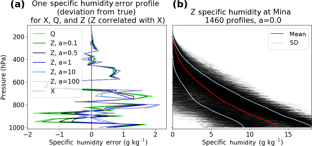
Figure 1(a) One set of error profiles with the unnormalized Xerr (dotted line), Qerr (solid lime green line) and Zerr (various solid lines for different values of correlation parameter a). Qerr is uncorrelated with Xerr. For a = 0, Zerr = Qerr and Zerr and Xerr are uncorrelated. As a increases, Zerr is increasingly correlated with Xerr and looks less like Qerr and more like Xerr. For very large a (a = 100), Zerr (light blue solid line) is almost equal to Xerr (dotted line). (b) 1460 profiles of the unnormalized data set Z with zero correlation with X (a=0).
3.2 Relationship of correlation, error variance and error covariance terms
The correlation coefficient r between the Xerr and Zerr is given by
where and are the mean values of Xerr and Zerr, respectively (zero in our error model), and and are the standard deviations of Xerr and Zerr given by
The relationship between the correlation coefficient and covariance between Xerr and Zerr is therefore
It can be shown that for this particular error model
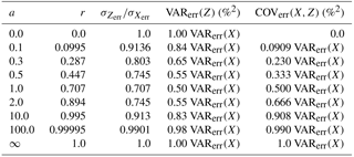
The correlation between X and Z errors can be varied according to Eq. (12) by varying the parameter a, as shown in Table 1. Note that VARerr(Z) ≤ VARerr(X) and that the maximum difference between VARerr(X) and VARerr(Z) occurs for a = 1 when VARerr(Z) = 0.5 VARerr(X) ( = 0.707 ).
Table 1Relationship between normalized error variances and standard deviations of data sets X and Z for different values of a.
3.3 Summary of generation of true data set and simulated data sets with random and systematic errors
-
We use 2007 ERA specific humidity q profiles for a location near Mina, Japan, which is located on Okinawa at 25.6∘ N, 131.5∘ W. There are four model data profiles per day or n=1460 profiles.
-
Assume each vertical profile of q has no error, and normalize the q at each level by the sample mean () at that level. This is the “true” data set.
-
Generate three different and independent random error profiles Xerr, Yerr and Qerr from Eqs. (8) and (9).
-
Generate Zerr for various specified values of a to control correlation using Eq. (10).
-
Add Xerr, Yerr and Zerr to true to obtain X, Y and Z, the 1460 simulated normalized profiles of q.
-
Compute the normalized estimated error variance profiles of X, Y and Z for the 3CH and 2CH methods according to Eqs. (3a)–(7a) (which have neglected all COV terms) and compare with the true error variances, which can be computed exactly from the full Eqs. (3)–(7) including the known values of the covariance terms. A value of a=0 should give the most accurate estimation of error variances because all covariance terms will be close to zero (they will not be exactly zero because the sample size n is finite).
We now derive expressions for the estimated values of the error variances for X, Y and Z for this error model and show how the correlations between Xerr and Zerr affect the approximate values using the 3CH and 2CH methods. This will give some insight into how correlations between actual observed data sets will affect estimates of their error variances and standard deviations. To make results more readily comparable to previous studies, instead of showing the error variance, we show the square root of the error variance, or the error standard deviation, in most figures.
4.1 Effect of error correlations on 3CH method
In the 3CH method, three covariance terms are neglected. These terms are zero for an infinite sample size for uncorrelated errors between the data sets. Correlation between the errors of two data sets will lead to a non-zero covariance term, which becomes larger for larger correlations. The error covariances COVerr(X,Z), COVerr(X,Y) and COVerr(Y,Z) are shown in Fig. 2 for a=0 and 0.5. Note that all error covariances oscillate around zero (and are zero for an infinitely large sample size) for a=0 (Fig. 2a). For a=0.5, the COVerr(X,Z) term increases with decreasing pressure, reaching a magnitude of about 800 %2 at 100 hPa (Fig. 2b).

Figure 2Vertical profiles of normalized error covariances (X,Y), (Y,Z) and (X,Z) for (a) a=0 and (b) a=0.5.
For our model (error correlation of X and Z) and an infinite sample size, COVerr(X,Z) is the only non-zero neglected term in Eq. (3a). Therefore Eq. (3a) can also be expressed as
Using Eq. (14) for this error model yields
Hence for a>0 the estimated error variance of X is always less than the true value, as seen in Fig. 3a.
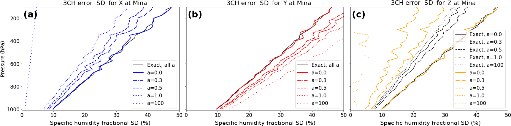
Figure 3(a) Estimated standard deviation of Xerr for values of a=0, 0.3, 0.5, 1.0 and 100 computed from Eqs. (3a)–(5a). Exact SD computed from data set X (solid black profile). (b) Same as (a) except for estimated SD of Yerr. (c) Same as (a) except for estimated SD of Zerr. Note that for different values of a, the exact SD of Xerr and Yerr are always the same. The exact SD of Zerr decreases as a increases for . For a>1.0, the exact SD of Zerr increases as a increases, becoming equal to the SD of Xerr for a=∞ due to the way our error model is defined (see also Table 1). For a=100 the correlation between X and Z errors is 0.99995 (Table 1; black dotted line for a=100 almost identical to black solid line for a=0).
We next consider the effect of the X and Z error correlation on the estimate for Y error variance. For our error model, Eq. (4a) can be expressed as
Substituting for the COV term from Eq. (14) and noting that, for our error model, VARerr(X) = VARerr(Y) we obtain
Thus the estimated error variance for Y is always greater that the true value for a>0, which is seen in Fig. 3b.
Lastly, we consider the effect of the X and Z correlation on the estimate for theZ error variance. Equation (5a) can be expressed as
Substituting for the COV term from Eq. (14) and using Eq. (13) we obtain
so that the estimated error variance for Z is less than the true value for a>0, which is illustrated in Fig. 3c. Finally, for a>1, Eq. 20 shows that the estimated error variance of Z is negative and the SD is undefined. For a=1.0, the estimated error variance of Z is zero for an infinite data set, but oscillates around zero because of our finite data set. Thus the estimated SD of Zerr is undefined at some levels (Fig. 3c).
4.2 Summary of error correlations on 3CH method
For the 3CH method, correlation between the data sets X and Z has the following affect on their computed error variances (when covariance terms are neglected):
-
VARerr(X)est< VARerr(X)true,
-
VARerr(Y)est> VARerr(Y)true,
-
VARerr(Z)est< VARerr(Z)true.
Figure 4 shows the ratios of the approximate error variances and standard deviations to the true values for a ranging from 0 to 1 for the 3CH method. As the correlation parameter a increases from 0, the differences between the estimated and true error variances increase. For a modest value of a=0.2 (correlation coefficient between X and Z errors of 0.196), the errors in the SD estimates are −9 % for X, +8 % for Y and −12 % for Z. As the correlation between the X and Z error reach 0.5, the percentage errors for the X, Y and Z estimates reach −18, +14.5 and −37 %, respectively. To the extent that this error model gives an idea of the effect of the correlation between the errors of two of the three data sets, estimates of error standard deviations using a large sample of real data should be accurate to within approximately 10 % for correlation coefficients between data errors of 0.2 or below, and within 25 % for correlation coefficients of around 0.3. The effect of the correlation between Z and X errors on the estimated error variance is greatest on the estimated Z error variance.
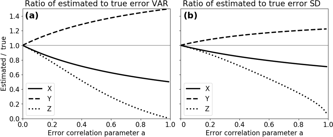
Figure 4Ratio of estimated (a) error variances to true variances and (b) estimated SD to true SD for the 3CH method for values of error correlation parameter a ranging from 0 to 1.0.
4.3 Effect of error correlations on 2CH method
We next examine how error correlations in our error model affect the 2CH method. To estimate the error variance of X using Eq. (6a), we calculate examples of the error terms for a=0 and a=0.5. The COVerr(X,Z) term was already shown in Fig. 2, and is the same in the 2CH method as in the 3CH method. Figures 5 and 6 show profiles of the other two terms for an error correlation between X and Z of a=0 and 0.5. In our error model Xerr and Zerr are uncorrelated with true, so the non-zero values in Figs. 5–6 are a result of the finite data set (1460 in this example). The COVerr(X,Z) (Fig. 2) increases as a increases, reaching a maximum value in the upper troposphere of about 800 %2 for a=0.5. The terms involving true and the errors in X, Y and Z in Figs. 5 and 6 do not change in magnitude with an increasing value of a, but they increase in amplitude with height and are significantly large (∼ 300 %2) compared to the COVerr(X,Z). These results indicate that a large sample size is especially important in the 2CH method, even with a sample size of 1460 the random errors caused by the neglect of the covariance terms involving true and the errors in X and Z can be significant.
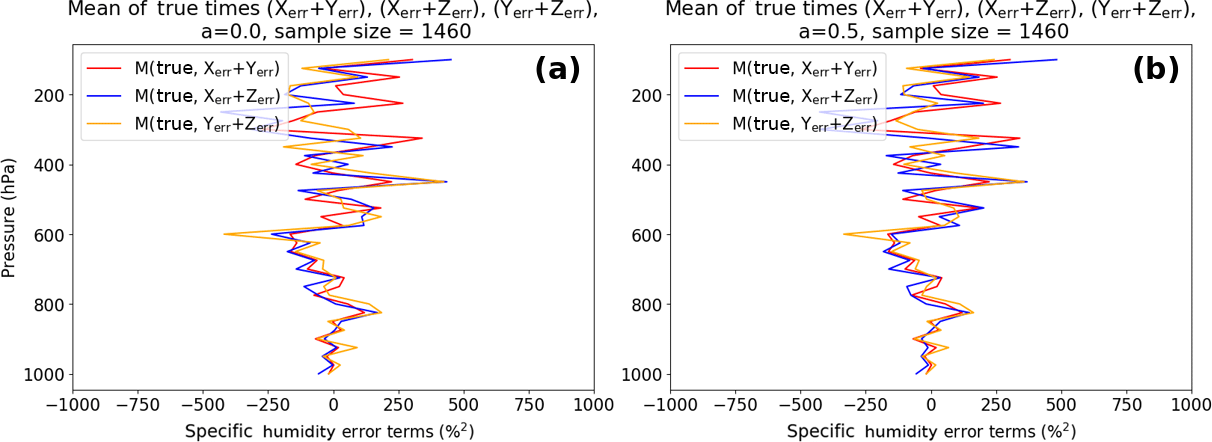
Figure 5Terms involving products of true and (Xerr + Zerr), (Xerr + Yerr) and (Yerr + Zerr) for (a) a=0 and (b) a=0.5. Note that the magnitudes of true and (Xerr + Yerr) and true and (Yerr + Zerr) do not depend on the correlation between Xerr and Zerr. All error terms are normalized.
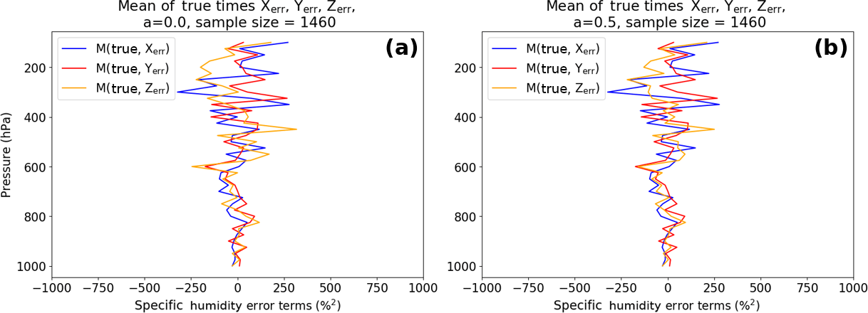
Figure 6Mean of products of true and Xerr, Yerr and Zerr for (a) a=0 and (b) a=0.5. All error terms are normalized.
Figure 7 shows the exact and estimated error SD of X, Y and Z for various combinations of the data sets and values of a. The estimated error SD for X, Y and Z vary around the exact solutions (black lines) for all values of a if data sets with uncorrelated errors are combined: (a) SDerr(X) computed with Y, (b) SDerr(Y) computed with X, (c) SDerr(Z) computed with Y and (e) SDerr(Y) using Z. Note that in (c) the exact SDerr(Z) decreases with a increasing from 0 to 1, as described previously. Figure 7d and f show how correlated errors between the data sets affect the estimated error variances. Both the estimated SDerr(X) and SDerr(Z) become too small when the data sets X and Z are combined and the value of a is increased. The exact solutions for all values of a in (Fig. 7f) are in black.
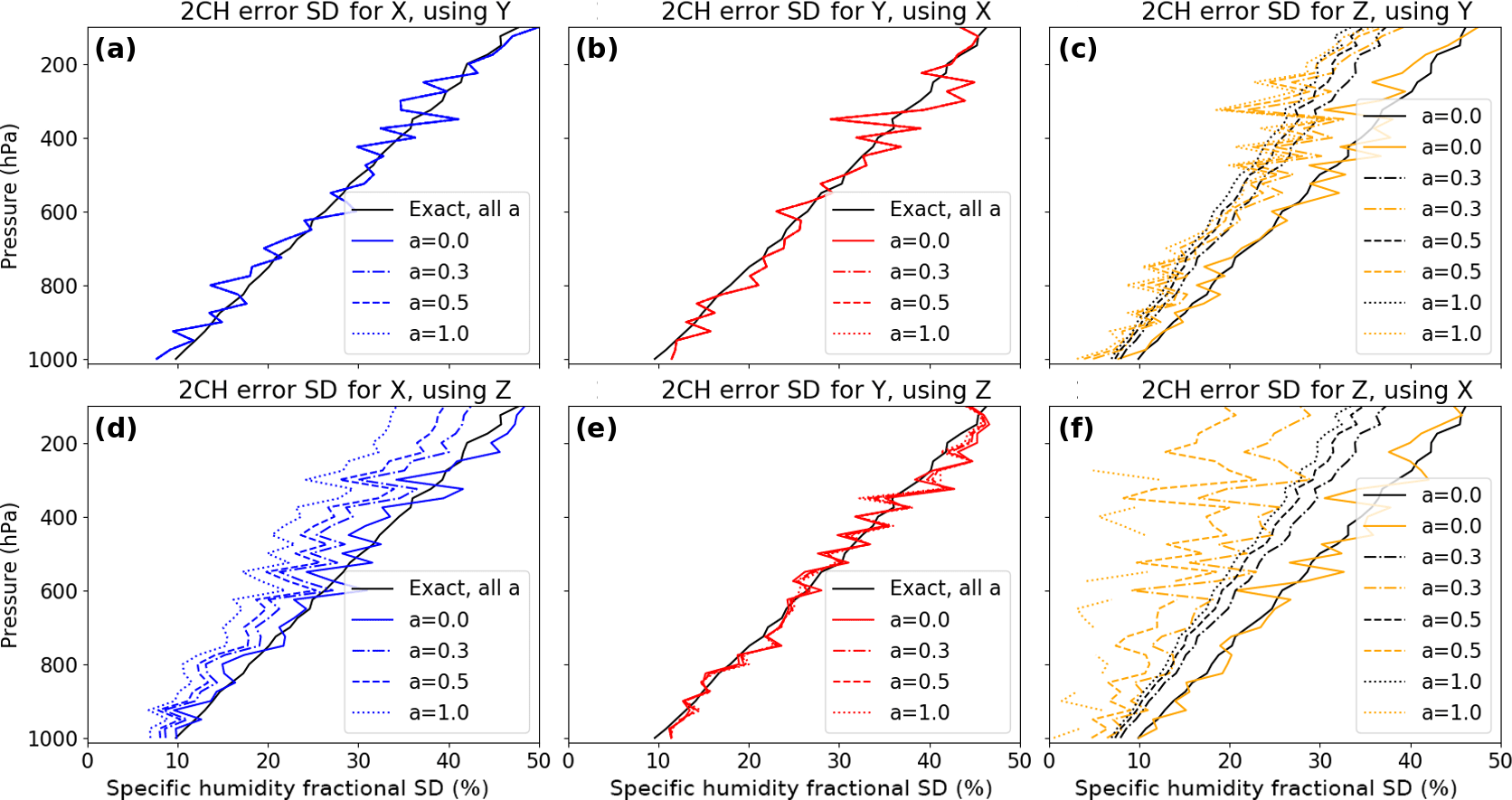
Figure 7Two 2CH results each for the normalized error SD for X (a, d), Y (b, e) and Z (c, f), depending on the second data set. Profiles corresponding to several values of correlation parameter a are included. The solid black profile is the exact error SD profile for X and Y for all values of a, and for Z when a=0.
4.4 Comparison of 3CH and 2CH methods using the error model
4.4.1 Effect of random errors
Figure 8 compares the normalized error estimates from the 3CH and 2CH methods for a=0.5. In Fig. 8a (3CH) the solid lines denote exact error SD of X, Y and Z. The exact error SD are the same for X and Y and are smaller for Z as discussed earlier. The estimated error SD (dashed lines) are less than the exact values for X and Z and greater than the exact values for Y, also as discussed earlier. In Fig. 8b (2CH), solid lines denote a combination of data sets with uncorrelated errors (where error terms are neglected, but are non-zero due to a finite sample size), while dashed lines indicate combinations of data sets with correlated errors and neglected error terms. We see that for the 3CH method and 2CH method all estimates are similar, with the exception of SDerr(Y), which is affected in the 3CH method by correlation of Xerr and Zerr. However, the profiles of the 2CH estimates show considerably more noise than those of the 3CH estimates, which is a consequence of the larger magnitude of the neglected error terms in the 2CH method (see Sects. 2.3 and 4 above).
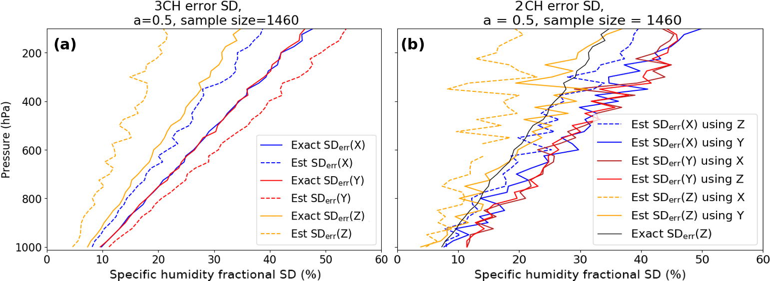
Figure 8Estimated and exact normalized error standard deviations for 3CH method (a) and 2CH method (b) for a correlation of Z and X errors of 0.45 (a=0.5). (a) Exact SD errors for X, Y and Z are given by blue, red and orange solid lines, respectively. Estimated error SD error is given by dashed lines of same color. (b) Exact error SD of Z is given by solid black line. Estimated error SD of X using Z and Y is given by blue lines, estimated error SD of Y using X and Z is given by red lines, and estimated error SD of Z using X and Y is given by orange lines. For all colored lines, error terms are neglected. Solid lines indicate estimates from combinations of data sets with uncorrelated errors, dashed lines indicate estimates from combinations of data sets with correlated errors and hence larger error terms.
We next consider the effect of the sample size on the error estimates from the 3CH and 2CH methods. We repeat the calculations from both methods by using a subset of the 1460 samples used in the above calculations. We created the subset by selecting every tenth sample from the complete set, giving a sample size of 146.
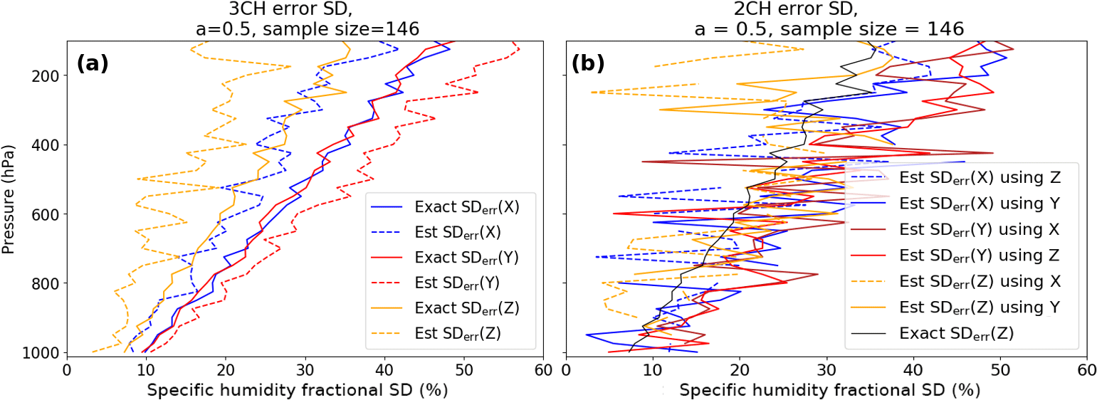
Figure 9Same as Fig. 8 except for a smaller sample size of 146. All profiles become much noisier, with the 2CH method showing significantly more noise than the 3CH method.
Figure 9 shows the same estimates as those in Fig. 8, except for the much smaller sample size of 146. For the smaller sample size, the noise increases for both methods. However, the effect on the 3CH method is less than on the 2CH method, and the differences in the estimates are still clearly visible in the 3CH method. For some of our comparison data sets using real data (Anthes and Rieckh, 2018), the sample size n is less than 100 in the lower and upper troposphere; hence the noise due to small sampling size is likely to be significant in the estimates for these regions.
4.4.2 Effect of bias errors
To investigate the effect of both random and systematic errors, we add a known bias ϵ to data set Z.
For the 3CH method, Eq. (3a) becomes
which may be expanded to
which is equal to Eq. (3a) plus the bias term. For random errors and a large sample size the means of Xerr and Yerr will be very small and the difference of the mean errors will also be small. Thus the bias term will tend toward zero as the sample size increases and the effect of a bias error in Z is minimal in the 3CH method.
This is not the case in the 2CH method, as shown below. Equation (6a) becomes
which can be expanded to
which is equal to Eq. (6a) plus a bias term.
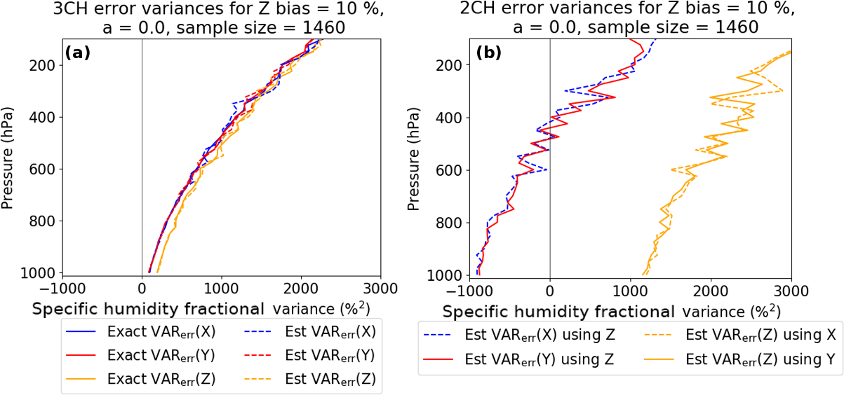
Figure 10Effect of adding a constant bias of 10 % to Z for the 3CH (a) and 2CH (b) methods, for no correlation between X and Z errors (i.e., a=0). The 3CH method yields reasonable estimates for all variables, while the estimated error variances from the 2CH method are erroneously large for Z (orange) and erroneously low X and Y (blue and red).
As noted above, the bias term in the 3CH method can be close to zero and therefore not affect the computed VARerr(X) significantly. The bias term of the 2CH method will stabilize with higher sample sizes around the product of the bias (ϵ) and the M(X) and will significantly influence the estimated error variance. A positive bias in the data set Z will cause a negative error in VARerr(X), and a negative bias in the data set Z will cause a positive error in VARerr(X).
For the simulated data set, Eq. (10) becomes
while Xerr and Yerr stay the same.
Figure 10 shows the effect of adding a constant bias of 10 % to Z for the 3CH and 2CH methods for no correlation of random errors (a=0). For the 3CH method (Fig. 10a), results still look reasonable, and the estimated and exact solutions overlap well. For the 2CH method (Fig. 10b), a bias of 10 % strongly impacts the estimated error variances. For Z, they are much too high, and for X and Y they are much too low. Recalling that the variables X, Y, Z and ϵ are all normalized by the sample mean , M(X) in Eq. (24) is approximately 100 %, so the term ϵ M(X) is approximately 100 ϵ %2. For ϵ=10 %, this term is 1000 %2, which is the offset we see for X, Y and Z in Fig. 10b.
4.4.3 General expression for effect of biases in all three data sets
More generally, we can derive expressions for the effect of biases of all three data sets with respect to true as follows (Sergey Sokolovskiy, personal communication, 2018): let
where ϵX, ϵY and ϵZ are biases of X, Y and Z, respectively. Substituting these expressions into Eq. (3a) for the 3CH method and Eq. (6a) for the 2CH method, we find that the difference Δ between the error estimates for X with biases and those without biases is
The first term of Eq. (29) is a first-order term while all the other terms are second order; thus in general biases will have a larger effect in the 2CH method compared to the 3CH method. We note that these expressions are valid only for an infinite data set.
Anthes and Rieckh (2018) showed a large number of error variance estimates using real data and the 3CH method at four RS locations in the Pacific Ocean region. Here we show a few examples of how the 2CH method compares with these 3CH estimates.
We use co-located data of RO, RS and ERA at Mina, which is one of the four RS stations studied by Anthes and Rieckh (2018) and Rieckh et al. (2018). We use the RO direct method for computing RO specific humidity (uses NCEP Global Forecast System temperature to compute specific humidity q from observed RO refractivity). Details about the co-location criteria and specific humidity retrieval are described by Rieckh et al. (2018).

Figure 11(a) Number of co-located measurements (data pairs) per pressure level for RO, RS and ERA. (b) Normalized q values for radiosondes (RS) at Mina, 2007. The normalized q values are computed as , where is the annual mean value of q for 2007. Profiles cut off at 250 hPa because RS data are not reported at higher levels. At the bottom, co-located profiles thin out since RO penetration depth varies and only very few profiles are available at the lowest levels.
To compute error variances using the 2CH method, Eq. (6a) is applied for various combinations of the four data sets. Data pairs at each level are only used when data are available for all four data sets. All data sets are interpolated to a common 25 hPa grid. Figure 11a shows the number of co-located profiles per pressure level. Figure 11b shows the normalized RS specific humidity values for these profiles.
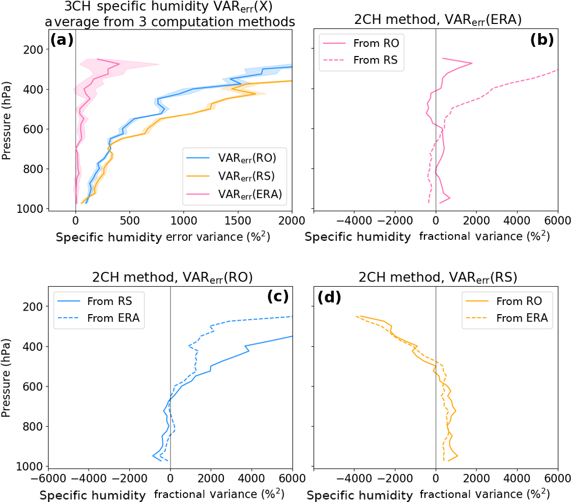
Figure 12Estimated error variances for specific humidity: (a) results from the 3CH method for ERA (purple), RO (blue) and RS (orange). Other three panels: 2CH method estimates for ERA (b), RO (c) and RS (d).
The two model and the RO data sets are representative of similar horizontal scales (∼ 100 km), while the RS data are in situ point measurements and therefore represent a much smaller horizontal scale. However, many studies (e.g., Ho et al., 2010a, b; Kuo et al., 2004; Chen et al., 2011) have used RS data as correlative data for verifying models, RO and other data sets without applying corrections for representativeness errors. These results indicate that the different representative scales are not a significant source of error in the comparisons (unlike spatial and temporal sampling errors resulting from the time and spatial differences between the data sets, which we correct for). However, any representativeness errors are included in the error estimates using either the 2CH or 3CH method.
All four data sets have some degree of unknown bias for certain locations, altitudes or atmospheric conditions; none of them represent the ultimate “truth” and there is no standard atmospheric data set for calibration. However, they have all been compared to other models or observations to one degree or another. We investigated the effect of biases in a related paper by Anthes and Rieckh (2018) by calibrating the data sets to the ERA data set using the scaling coefficients as given by Stoffelen (1998) and Vogelzang et al. (2011). The results using the calibrated data sets were very similar to those using the uncalibrated data sets, confirming that the 3CH method is insensitive to small biases.
We use our results from the 3CH method for real data (Anthes and Rieckh, 2018) to evaluate the results of the 2CH method. Figure 12a shows the 3CH estimated error variances for specific humidity for ERA, RS and RO using three independent equations (Anthes and Rieckh, 2018). The mean value of the estimates is given by the solid line and the SD of the estimates about the mean by the shading. The 3CH estimates are considered reasonably accurate for the reasons given in Anthes and Rieckh (2018), namely that the magnitude and shape of the estimates for refractivity agree with other independent refractivity error estimates (so we assume that the method works just as well for humidity as for refractivity), and that the results are consistent for the four different RS stations studied.
The other panels in Fig. 12 show the 2CH estimates of the error variance for ERA (b), RO (c) and RS (d) using various pairs of observations. We consider the 2CH estimates unrealistic for these data sets. The magnitudes reach values that are negative or up to 5 times the magnitudes of the 3CH method, which is considered unrealistically large. The profiles of the estimates of error variances of ERA, RS and RO are also quite different depending on the pairs of observations used, unlike the 3CH method in which all combinations of observations give similar profiles. Similar results were obtained for 2CH estimates of refractivity (not shown).
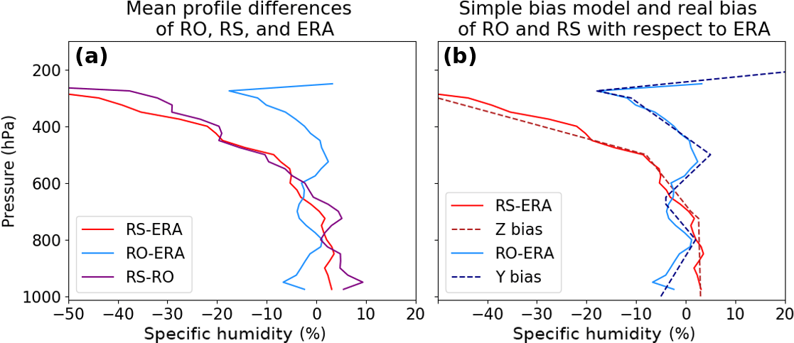
Figure 13(a) Annual mean normalized profiles of RS–ERA, RO–ERA and RS–RO. (b) Same for RS–ERA and RO–ERA only (solid lines), and their respective empirical bias profiles (dashed lines) based on the mean profiles.
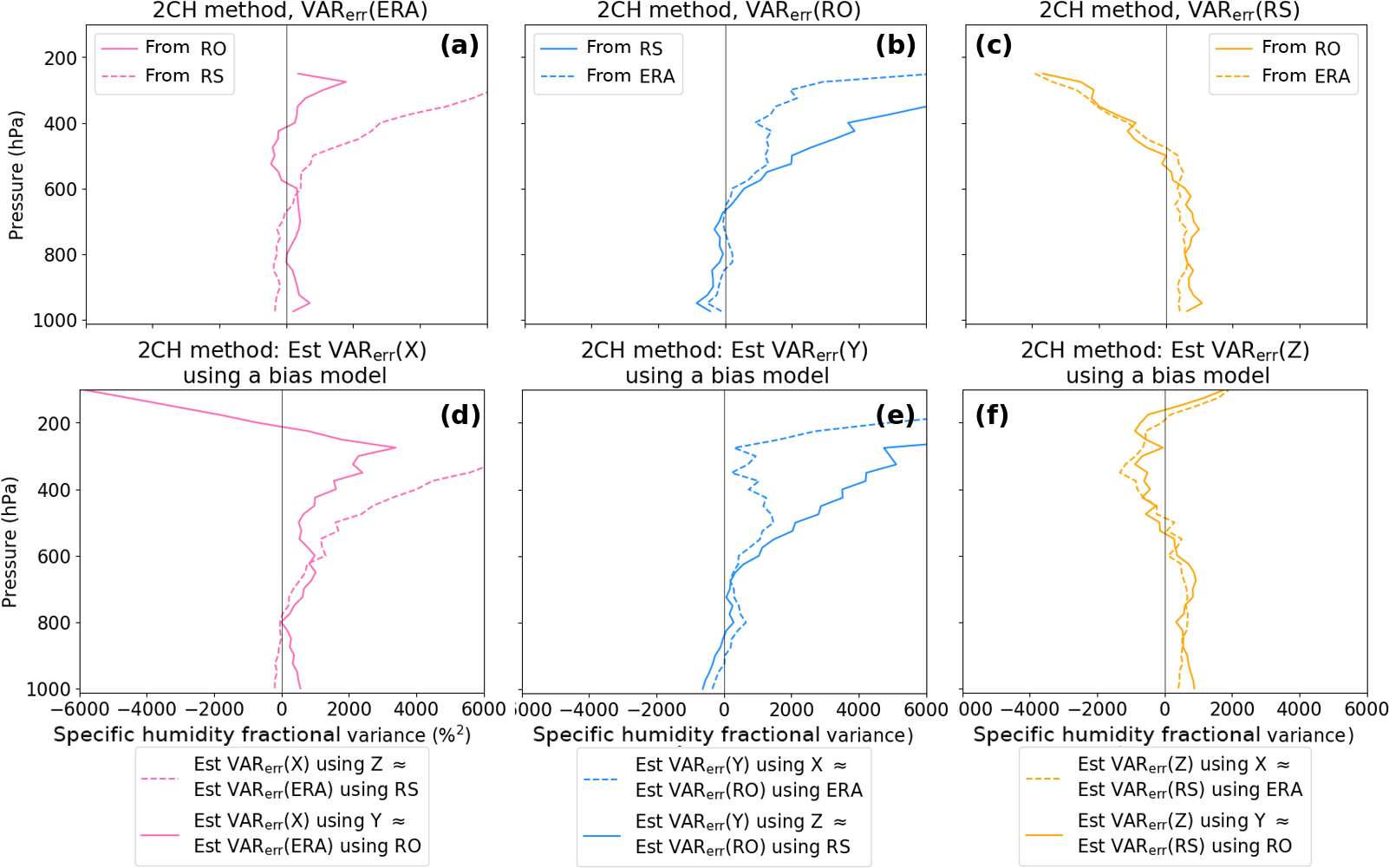
Figure 142CH method error variances for ERA, RO and RS (a–c) and for simulated data using the specified empirical bias profiles (d–f). Correlation between X and Z errors is zero for this experiment.
Thus we find that the 2CH method produces estimates of the error variances for specific humidity that are quite different from those of the 3CH method. We suspected that the cause for the different behavior using real data might lie in the different treatment of bias errors in the 2CH and 3CH method. To investigate this hypothesis, we considered the effect of an empirically based bias in the simulated data.
5.1 Simulating the observed real data bias in the 2CH method
As shown in Sect. 4.4.2, even small bias errors in one of the data sets can cause large errors in the 2CH method. To see whether a bias in our real data could explain the very different estimates of the error variances shown in Fig. 12b–d for the 2CH method, we set up empirically based bias profiles in the simulated data. These match approximately the observed differences of RS and RO from ERA as found by Rieckh et al. (2018) in the real data sets (Supplement, Fig. S5 panel 4 for RS; Fig. S6 panel 1 for RO). For the tests we consider ERA the truth. We computed the specific humidity annual mean biases of RO and RS for each level as 100[mean(RO) − mean(ERA)]∕mean(ERA) and 100[mean(RS) − mean(ERA)]∕mean(ERA), respectively. We used these results to create a simple additive bias for both Y and Z. The biases are depicted in Fig. 13 (dashed lines), along with the real RS and RO annual mean biases (solid lines). More specifically, the bias used for Y (simulating the RO bias) varies linearly between pressure levels as
-
−5 to 2 % from 1000 to 800 hPa
-
2 to −4 % from 800 to 650 hPa
-
−4 to 5 % from 650 to 500 hPa
-
5 to −11 % from 500 to 300 hPa.
The bias used for Z (simulating the RS bias) varies linearly between pressure levels as
-
3 to 1 % from 1000 to 700 hPa
-
1 to −8 % from 700 to 500 hPa
-
−8 to −50 % from 500 to 300 hPa.
The respective bias is added to both Y and Z when the data are created from the true profiles:
We use these specified biased data sets to compute error variances via the 2CH method. Results are shown in Fig. 14, with the results of the real data in the top row (a–c) and the results of the simulated bias data in the bottom row (d–f).
The error variances of the simulated biased data sets (bottom row) are quite similar to the error variances estimated with the real data (top row), indicating that biases are largely responsible for the results using real data and how they vary from the 3CH method results.
In this study we compared two methods for estimating the error variances of multiple data sets, the three-cornered hat (3CH) and two-cornered hat (2CH) methods. Using a simulated data set in which we could vary the degree of correlation between two data sets as well as specifying bias errors, we examined the sensitivity of the 3CH and 2CH methods to random and bias errors. For the error model, we added known random or bias errors to 1460 specific humidity profiles (considered truth) obtained from the ERA-Interim reanalysis (ERA) over a subtropical radiosonde (RS) station in Japan. We compared the effect of neglecting various error covariance and other error terms in the 3CH and 2CH methods on the estimated error variances and standard deviations. We also considered the effect of a finite sample size on the estimates by repeating the calculations using a subset of 146 of the total 1460 profiles. We found that the 3CH method was less sensitive to the neglected error terms for various random error correlations than the 2CH method. We also showed that the effect of bias errors on one of the data sets had a relatively small effect on the 3CH method, but produced much larger errors in the 2CH method.
We also compared the 3CH and 2CH methods using real RS, radio occultation (RO) and ERA data. We find that the 3CH method produces more consistent and accurate results than the 2CH method when using real data. The 2CH method produced very different estimates of the error variance of ERA depending on which observational data set (e.g., RS or RO) was used in the comparison. Using an empirical bias model based on observed RS and RO difference from ERA during 2007, we showed that these differences in error variance estimates were likely caused by different biases in the RS and RO data. The effect of bias errors is shown to give unrealistic results using the 2CH method.
Code will be made available by the author upon request.
Data can be made available from authors upon request.
In the 2CH method, sums and differences of two data sets X and Z are used to derive the error variances of X and Z.
Equation (A3) is summed over all the data pairs to get
Defining the following expressions:
Eq. (A4) becomes
We then subtract Z from X and square the difference to get
Finally, we solve for MS(true) by subtracting Eq. (A6) from Eq. (A5):
By squaring the expression X= (true +Xerr) we get the exact expression for the VARerr(X):
and substituting for MS(true) from Eq. (A7) gives
Similarly, we obtain
We note that the top lines in Eqs. (A9) and (A10) may be written as VAR) and VAR, which are the forms used by Stoffelen (1998) and Vogelzang et al. (2011).
Both authors contributed equally to the ideas and conceptual development. The first author computed the results.
The authors declare that they have no conflict of interest.
The authors were supported by NSF-NASA grant AGS-1522830. We thank
Shay Gilpin for Fig. 4 and the two reviewers for their comments on
the original draft. John Eyre (Met Office) provided useful insights and comments on drafts of the manuscript. We thank Eric DeWeaver (NSF) and Jack Kaye (NASA)
for their long-term support of COSMIC.
Edited by: Ad Stoffelen
Reviewed by: two anonymous referees
Anthes, R. and Rieckh, T.: Estimating observation and model error variances using multiple data sets, Atmos. Meas. Tech., 11, 4239–4260, https://doi.org/10.5194/amt-11-4239-2018, 2018. a, b, c, d, e, f, g, h, i, j, k
Braun, J., Rocken, C., and Ware, R.: Validation of line-of-sight water vapor measurements with GPS, Radio Sci., 36, 459–472, 2001. a, b, c
Chen, S.-Y., Huang, C.-Y., Kuo, Y.-H., and Sokolovskiy, S.: Observational Error Estimation of FORMOSAT-3/COSMIC GPS Radio Occultation Data, Mon. Weather Rev., 139, 853–865, https://doi.org/10.1175/2010MWR3260.1, 2011. a, b
Collard, A. D. and Healy, S. B.: The combined impact of future space-based atmospheric sounding instruments on numerical weather-prediction analysis fields: A simulation study, Q. J. Roy. Meteor. Soc., 129, 2741–2760, https://doi.org/10.1256/qj.02.124, 2003. a, b
Dee, D. P., Uppala, S. M., Simmons, A. J., Berrisford, P., Poli, P., Kobayashi, S., Andrae, U., Balmaseda, M. A., Balsamo, G., Bauer, P., Bechtold, P., Beljaars, A. C. M., van de Berg, L., Bidlot, J., Bormann, N., Delsol, C., Dragani, R., Fuentes, M., Geer, A. J., Haimberger, L., Healy, S. B., Hersbach, H., Hólm, E. V., Isaksen, L., Kållberg, P., Köhler, M., Matricardi, M., McNally, A. P., Monge-Sanz, B. M., Morcrette, J.-J., Park, B.-K., Peubey, C., de Rosnay, P., Tavolato, C., Thépaut, J.-N., and Vitart, F.: The ERA-Interim reanalysis: configuration and performance of the data assimilation system, Q. J. Roy. Meteor. Soc., 137, 553–597, https://doi.org/10.1002/qj.828, 2011. a
Desroziers, G. and Ivanov, S.: Diagnosing and adaptive tuning of observation-error parameters in a variational assimilation, Q. J. Roy. Meteor. Soc., 127, 1433–1452, https://doi.org/10.1002/qj.49712757417, 2001. a
Ekstrom, C. R. and Koppang, P. A.: Error Bars for Three-Cornered Hats, IEEE Trans. Ultrason. Ferroelect. Freq. Contr., 53, 876–879, https://doi.org/10.1109/TUFFC.2006.1632679, 2006. a
Gray, J. E. and Allan, D. W.: A method for estimating the frequency stability of an individual oscillator, Atlantic City, New Jersey, 29–31 May, 1974. a, b
Griggs, E., Kursinski, E., and Akos, D.: An investigation of GNSS atomic clock behaviour at short time intervals, GPS Solut., 18, 443–452, https://doi.org/10.1007/s10291-013-0343-7, 2014. a, b
Griggs, E., Kursinski, E., and Akos, D.: Short-term GNSS satellite clock stability, Radio Sci., 50, 813–826, https://doi.org/10.1002/2015RS005667, 2015. a
Gruber, A., Su, C.-H., Zwieback, S., Crow, W., Dorigo, W., and Wagner, W.: Recent advances in (soil moisture) triple collocation analysis, Int. J. Appl. Earth Obs. Geoinf., 45, 200–211, https://doi.org/10.1016/j.jag.2015.09.002, 2016. a
Ho, S.-P., Kuo, Y.-H., Schreiner, W., and Zhou, X.: Using SI-traceable Global Positioning System radio occultation measurements for climate monitoring, B. Am. Meteorol. Soc., 91, S36–S37, 2010a. a
Ho, S.-P., Zhou, X., Kuo, Y.-H., Hunt, D., and Wang, J.-H.: Global evaluation of radiosonde water vapor systematic biases using GPS radio occultation from COSMIC and ECMWF analysis, Remote Sens., 2, 1320–1330, https://doi.org/10.3390/RS2051320, 2010b. a
Kuo, Y.-H., Wee, T.-K., Sokolovskiy, S., Rocken, C., Schreiner, W., Hunt, D., and Anthes, R. A.: Inversion and error estimation of GPS radio occultation data, J. Meteor. Soc. JPN, 82, 507–531, 2004. a, b
Kursinski, E. R., Hajj, G. A., Schofield, J. T., Linfield, R. P., and Hardy, K. R.: Observing Earth's atmosphere with radio occultation measurements using the Global Positioning System, J. Geophys. Res., 102, 23429–23465, https://doi.org/10.1029/97JD01569, 1997. a
Luna, D., Pérez, D., Cifuentes, A., and Gómez, D.: Three-Cornered Hat Method via GPS Common-View Comparisons, IEEE Trans. Instrument. Measure., 66, 2143–2147, https://doi.org/10.1109/TIM.2017.2684918, 2017. a
O'Carroll, A. G., Eyre, J. R., and Saunders, R. S.: Three-way error analysis between AATSR, AMSR-E, and in situ sea surface temperature observations, J. Atmos. Ocean. Technol., 25, 1197–1207, https://doi.org/10.1175/2007JTECHO542.1, 2008. a, b
Rieckh, T., Anthes, R., Randel, W., Ho, S.-P., and Foelsche, U.: Evaluating tropospheric humidity from GPS radio occultation, radiosonde, and AIRS from high-resolution time series, Atmos. Meas. Tech., 11, 3091–3109, https://doi.org/10.5194/amt-11-3091-2018, 2018. a, b, c, d
Riley, W. J.: Application of the 3-cornered hat method to the analysis of frequency stability, available at: http://www.wriley.com/3-CornHat.htm (1 July 2018), 2003. a, b
Roebeling, R. A., Wolters, E. L. A., Meirink, J. F., and Leijnse, H.: Triple collocation of summer precipitation retrievals from SEVIRI over Europe with gridded rain gauge and weather radar data, J. Hydrometeorol., 13, 1552–1566, https://doi.org/10.1175/JHM-D-11-089.1, 2012. a
Stoffelen, A.: Toward the true near-surface wind speed: Error modeling and calibration using triple collocation, J. Geophys. Res., 103, 7755–7766, https://doi.org/10.1029/97JC03180, 1998. a, b, c, d, e
Su, C.-H., Ryu, D., Crow, W. T., and Western, A. W.: Beyond triple collocation: Applications to soil moisture monitoring, J. Geophys. Res., 119, 6419–6439, https://doi.org/10.1002/2013JD021043, 2014. a
Valty, P., de Viron, O., Panet, I., Camp, M. V., and Legrand, J.: Assessing the precision in loading estimates by geodetic techniques in Southern Europe, Geophys. J. Int., 194, 1441–1454, https://doi.org/10.1093/gji/ggt173, 2013. a
Vogelzang, J., Stoffelen, A., Verhoef, A., and Figa-Saldaña, J.: On the quality of high-resolution scatterometer winds, J. Geophys. Res., 116, C10033, https://doi.org/10.1029/2010JC006640, 2011. a, b, c
von Engeln, A. and Nedoluha, G.: Retrieval of temperature and water vapor profiles from radio occultation refractivity and bending angle measurements using an Optimal Estimation approach: a simulation study, Atmos. Chem. Phys., 5, 1665–1677, https://doi.org/10.5194/acp-5-1665-2005, 2005. a
Wang, B.-R., Liu, X.-Y., and Wang, J.-K.: Assessment of COSMIC radio occultation retrieval product using global radiosonde data, Atmos. Meas. Tech., 6, 1073–1083, https://doi.org/10.5194/amt-6-1073-2013, 2013. a
- Abstract
- Introduction
- Error estimates using the 2CH and 3CH methods
- Generation of true data set and three simulated data sets with errors
- Effect of error correlations on estimated error variances
- Estimates of error variances using 3CH and 2CH methods and real observations
- Summary and conclusions
- Code availability
- Data availability
- Appendix A: Derivation of the 2CH method
- Author contributions
- Competing interests
- Acknowledgements
- References