the Creative Commons Attribution 4.0 License.
the Creative Commons Attribution 4.0 License.
 | 15 Aug 2018
Separation of the optical and mass features of particle components in different aerosol mixtures by using POLIPHON retrievals in synergy with continuous polarized Micro-Pulse Lidar (P-MPL) measurements
Carmen Córdoba-Jabonero
Michaël Sicard
Albert Ansmann
Ana del Águila
Holger Baars
The application of the POLIPHON (POlarization-LIdar PHOtometer Networking) method is presented for the first time in synergy with continuous 24/7 polarized Micro-Pulse Lidar (P-MPL) measurements to derive the vertical separation of two or three particle components in different aerosol mixtures, and the retrieval of their particular optical properties. The procedure of extinction-to-mass conversion, together with an analysis of the mass extinction efficiency (MEE) parameter, is described, and the relative mass contribution of each aerosol component is also derived in a further step. The general POLIPHON algorithm is based on the specific particle linear depolarization ratio given for different types of aerosols and can be run in either 1-step (POL-1) or 2 steps (POL-2) versions with dependence on either the 2- or 3-component separation. In order to illustrate this procedure, aerosol mixing cases observed over Barcelona (NE Spain) are selected: a dust event on 5 July 2016, smoke plumes detected on 23 May 2016 and a pollination episode observed on 23 March 2016. In particular, the 3-component separation is just applied for the dust case: a combined POL-1 with POL-2 procedure (POL-1/2) is used, and additionally the fine-dust contribution to the total fine mode (fine dust plus non-dust aerosols) is estimated. The high dust impact before 12:00 UTC yields a mean mass loading of 0.6±0.1 g m−2 due to the prevalence of Saharan coarse-dust particles. After that time, the mean mass loading is reduced by two-thirds, showing a rather weak dust incidence. In the smoke case, the arrival of fine biomass-burning particles is detected at altitudes as high as 7 km. The smoke particles, probably mixed with less depolarizing non-smoke aerosols, are observed in air masses, having their origin from either North American fires or the Arctic area, as reported by HYSPLIT back-trajectory analysis. The particle linear depolarization ratio for smoke shows values in the 0.10–0.15 range and even higher at given times, and the daily mean smoke mass loading is 0.017±0.008 g m−2, around 3 % of that found for the dust event. Pollen particles are detected up to 1.5 km in height from 10:00 UTC during an intense pollination event with a particle linear depolarization ratio ranging between 0.10 and 0.15. The maximal mass loading of Platanus pollen particles is 0.011±0.003 g m−2, representing around 2 % of the dust loading during the higher dust incidence. Regarding the MEE derived for each aerosol component, their values are in agreement with others referenced in the literature for the specific aerosol types examined in this work: 0.5±0.1 and 1.7±0.2 m2 g−1 are found for coarse and fine dust particles, 4.5±1.4 m2 g−1 is derived for smoke and 2.4±0.5 m2 g−1 for non-smoke aerosols with Arctic origin, and a MEE of 2.4±0.8 m2 g−1 is obtained for pollen particles, though it can reach higher or lower values depending on predominantly smaller or larger pollen grain sizes. Results reveal the high potential of the P-MPL system, a simple polarization-sensitive elastic backscatter lidar working in a 24/7 operation mode, to retrieve the relative optical and mass contributions of each aerosol component throughout the day, reflecting the daily variability of their properties. In fact, this procedure can be simply implemented in other P-MPLs that also operate within the worldwide Micro-Pulse Lidar Network (MPLNET), thus extending the aerosol discrimination at a global scale. Moreover, the method has the advantage of also being relatively easily applicable to space-borne lidars with an equivalent configuration such as the ongoing Cloud-Aerosol LIdar with Orthogonal Polarization (CALIOP) on board NASA CALIPSO (Cloud-Aerosol Lidar and Infrared Pathfinder Satellite Observation) and the forthcoming Atmospheric Lidar (ATLID) on board the ESA EarthCARE mission.
- Article
(4705 KB) - Full-text XML
- BibTeX
- EndNote


It is widely known that atmospheric aerosols contribute to climate change due to their effects (direct and indirect) on the Earth's energy budget. Different types of aerosols present different radiative properties and thus contribute in different ways to climate change (Boucher et al., 2013; Myhre et al., 2013). As far as estimates of aerosol direct radiative forcing are concerned, knowledge of the aerosol types under study is thus critical. The aerosol direct radiative properties involved in radiative transfer calculations are the particle extinction (scattering and absorption) coefficient, single-scattering albedo (the ratio of scattering to extinction), the asymmetry factor as defined as the intensity-weighted average cosine of the scattering angle and their vertical distribution. Referring to the important factors in constraining the radiative effect of aerosols, Boucher et al. (2013) stated, “Particularly important are the single-scattering albedo (especially over land or above clouds) and the AOD”. The AOD is aerosol optical depth, i.e. the column-integrated aerosol extinction. These two parameters can be estimated by or recalculated from the output of lidar stand-alone algorithms such as Müller et al. (1999), Veselovskii et al. (2002) or Böckmann et al. (2005) which employ state-of-the-art elastic-Raman lidar measurements at several wavelengths. Such advanced measurements are scarce, however, compared with the large database of elastic lidar measurements worldwide.
For this reason, synergetic algorithms recently combine data from multi-wavelength elastic lidar and passive instrumentation to retrieve the extinction or both the extinction and the single-scattering albedo at several wavelengths and discriminate between fine and coarse mode. These algorithms are the Lidar-Radiometer Inversion Code (LIRIC; Chaikovsky et al., 2016) and the Generalized Aerosol Retrieval from Radiometer and Lidar Combined data (GARRLiC; Lopatin et al., 2013). GARRLiC is embedded in a more generalized algorithm called the Generalized Retrieval of Atmosphere and Surface Properties inversion code (GRASP; Dubovik et al., 2014). The drawback of these algorithms is that they apply to at least 3-wavelength elastic systems, while a majority of single- and dual-wavelength elastic systems are operating worldwide. For less sophisticated systems, the primary way of discriminating between aerosol types is to have a polarization-sensitive channel, wherein the discrimination is based on the comparison of the particle depolarization ratio measured with two reference particle depolarization ratio values.
Aerosol discrimination using particle depolarization was first formulated by Chen et al. (2001) and then used by Shimizu et al. (2004) for the observation of Asian dust in China and Japan with one elastic and one depolarization sensitive channel. Since 2009, the method has been used in an increasing number of studies to discriminate between dust and smoke (Tesche et al., 2011), ash and fine-mode particles (Ansmann et al., 2011; 2012; Sicard et al., 2012), and pollen and background particles (Noh et al., 2013; Sicard et al., 2016a). Very recently, this method, known as the POlarization-LIdar PHOtometer Networking method (POLIPHON), has been refined by Mamouri and Ansmann (2014) to retrieve up to three aerosol components, such as fine and coarse dust and non-dust particles. POLIPHON is also the basis of the retrieval of ice nuclei number concentration in desert dust layers (Mamouri and Ansmann, 2015) and cloud condensation nucleus number concentration (Mamouri and Ansmann, 2016). In addition, a similar method is used for separating aerosol mixtures in HSRL systems (Burton et al., 2012, 2014).
In addition to their effects on climate, atmospheric aerosols are known to have a significant impact on human health when they are inhaled. For example, exposure to anthropogenic particles (pollution) is clearly identified as a public health hazard causing acute and chronic effects to the respiratory and cardiovascular systems (Dockery et al., 1993; Künzli et al., 2000; WHO, 2003). Airborne pollen grains produced by wind-pollinated plants are responsible for allergenic reactions when inhaled by humans (Cecchi, 2013). More recently, Martiny and Chiapello (2013) highlighted the role of desert dust on meningitis epidemics. Toxicological studies are currently aiming to identify which particle characteristics are responsible for which adverse health effects (e.g. particle number, mass, size, surface, chemical composition). Among these properties, the aerosol that lidars can probably estimate the best is mass concentration, when the aerosol type has been previously identified, and thus the relation between aerosol backscatter and extinction can be accurately related to specific aerosol physical properties. However, mass concentration retrievals from lidar data are not common and there is very little information available on the vertical distribution of aerosol number and mass concentrations, although a number of field experiments involving research and commercial aircraft have measured aerosol concentrations (Heintzenberg et al., 2011).
Mass concentration profiles can be estimated by multiplying the lidar-derived extinction coefficient by the mass extinction efficiency, sometimes also called the specific extinction cross section, when the latter is known or can be assumed. This conversion is often used to convert lidar-derived optical properties into mass concentration to test and evaluate transport models (Pérez et al., 2006; Sicard et al., 2015). Lately, POLIPHON is also used to extract the fractions of the high, moderate or low depolarizing particles from the total extinction, which can then be converted separately into mass concentration (Mamouri and Ansmann, 2014, 2017). The method has been used for the estimation of the profile of mass concentration of dust (Ansmann et al., 2011, 2012), volcanic ash (Ansmann et al., 2012; Sicard et al., 2012) and pollen (Sicard et al., 2016b). It is worth mentioning that another field that would greatly benefit from the knowledge of the aerosol mass concentration profile is the air traffic, as large particles can damage aircraft engines. By way of example, we recall the impact of the ash-loaded eruption plume from the Icelandic Eyjafjallajökull volcano on European air traffic in 2010 (Pappalardo et al., 2013).
The aim of this paper is to show the potential of simple lidar systems, with one elastic and one depolarization sensitive channel, to discriminate between several aerosol types and retrieve the profiles of their optical properties and mass concentrations for each aerosol component. The instrument used is the polarized version of the Micro-Pulse Lidar (P-MPL), the standard system within NASA MPLNET (Micro Pulse Lidar Network; MPLNET, 2016), situated at the Universitat Politècnica de Catalunya (UPC) at Barcelona (BCN) in north-eastern Spain. The P-MPL is an elastic and monochromatic low-energy system which also includes a depolarization-sensitive channel, operating in an automatic and continuous 24/7 mode. The algorithm used to optically discriminate components in aerosol mixtures is the POLIPHON method, both 1-step and 2-step versions, in order to assess the vertical separation of a maximum of three aerosol components. The synergetic use of P-MPL/POLIPHON is tested with aerosol mixtures containing specific climate-relevant aerosols, namely desert dust, fire smoke and pollen. This is the first time that POLIPHON, which well established for sophisticated powerful European Aerosol Research Lidar NETwork (EARLINET) lidars, is applied to worldwide (MPLNET) and continuous simple elastic P-MPL measurements. Moreover, the method has the advantage of also being relatively easily applicable to space-borne lidars with an equivalent configuration such as the ongoing Cloud-Aerosol Lidar with Orthogonal Polarization (CALIOP) on board NASA CALIPSO (Cloud-Aerosol Lidar and Infrared Pathfinder Satellite Observations) which has two elastic and one depolarization-sensitive channel, and the forthcoming Atmospheric Lidar (ATLID) on board EarthCARE (future ESA mission to be launched in 2019), which will have a high spectral resolution receiver and a depolarization channel.
The paper is organized as follows: Sect. 1 presents the introductory framework. The methodology is introduced in Sect. 2, which breaks down into the description of the measurement station and of the selected aerosol cases (Sect. 2.1) as well as the lidar system used in this paper (Sect. 2.2), an extended overview of the POLIPHON method (Sect. 2.3) and a detailed extinction-to-mass conversion procedure (Sect. 2.4). Sect. 3 shows the results and their discussion for each case (dust, smoke and pollen). Finally, a summary of the work and the main conclusions are presented in Sect. 4. In addition, a list of acronyms (symbols) identifying the parameters and variables used in the work is shown in Appendix A.
2.1 Measurement station and selected aerosol case studies
Barcelona (BCN) station is an urban site located on the north-eastern Iberian Peninsula (41.4∘ N, 2.1∘ E, 115 m a.s.l.), along the coast of the Mediterranean Sea, on the north campus of UPC at the centre of Barcelona. The typical background aerosol is a mixture of pollution particles with a minor contribution of marine aerosols, but this is only predominant under particular clean conditions. Other aerosol types, such as desert dust, fire smoke and pollen are also frequently found (Sicard et al., 2011). BCN is a well-established EARLINET station, and a relatively new MPLNET site, where a polarized Micro-Pulse Lidar (P-MPL) has been in routine operation since 2014. BCN is also a NASA AERONET (AErosol RObotic NETwork, AERONET, 2017) site, measuring AOD and the column-integrated aerosol optical properties during the daytime (Holben et al., 1999).
Table 1Relative uncertainties for the P-MPL-derived particle optical properties (at 532 nm wavelength) and mass concentrations. (n) and (d) stand for night-time and daytime P-MPL measurements.
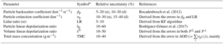
* As denoted in the text.
In this work, three case studies on different aerosol mixtures (dust, fire smoke and pollen, all mixed with local background aerosols) observed over BCN are examined in order to introduce the combined application of POLIPHON in synergy with continuous P-MPL measurements for the separation of, in particular, Saharan dust, fire smoke and pollen particles from other aerosols mixed with them. Those selected dust, smoke and pollen cases occurred on 5 July, 23 May and 23 March 2016, respectively. HYSPLIT back-trajectory (Hybrid Single Particle Lagrangian Integrated Trajectory model version 4 developed by the NOAA's Air Resources Laboratory (ARL); Draxler and Hess, 1998; Stein et al., 2015; Rolph et al., 2017) analysis is used to confirm the presence of dust and smoke over BCN for each particular case. HYSPLIT back trajectories are calculated for those days ending over BCN at given altitudes and several times in relation with the results obtained and discussed later in Sect. 3 for the dust and smoke cases.
The 5-day back-trajectory analysis indicates Saharan air masses arriving at high altitudes (>2000 m a.g.l.) on 5 July 2016 only before 12:00 UTC, North Atlantic air masses are simultaneously arriving at lower heights (see Fig. 1a–c); during the time period after 12:00 UTC, air masses at all altitudes are mostly coming from North Atlantic and central Spain regions (see Fig. 1d–f) but not from Saharan desert. On the other hand, smoke plumes detected on 23 May 2016 over BCN seem to be arriving from North America fires using 10-day back trajectories; depending on the altitude and time of the arrival, air masses are coming from either Canada and USA areas carrying fine biomass-burning particles or Arctic region with larger aerosols in comparison with those smoke particles (see Fig. 1g–l). The pollen case was selected as the day with the highest peak of daily pollen concentration in the period March–April. This peak occurred on 23 March 2016 and the most abundant taxon was Platanus. Belmonte (2016) counted a near-surface concentration of around 1700 grains of Platanus taxon per cubic metre in central Barcelona on 23 March 2016. This value is close to the daily values found in the pollination event of March 2015 in Barcelona described by Sicard et al. (2016a) as particularly strong in terms of pollen concentration. These results will be discussed in detail together with those obtained for each aerosol case in Sect. 3.
2.2 Polarized Micro-Pulse Lidar (P-MPL) system
The polarized Micro-Pulse Lidar system (P-MPL v. 4B, Sigma Space Corp.) acquires vertical aerosol profiles with a relatively high frequency (2500 Hz) using a low-energy (∼7 µJ) Nd:YLF laser at 532 nm. The P-MPL acquisition settings follow the NASA MPLNET requirements of 30 s integrating time and 15 m vertical resolution. Polarization capabilities rely on the collection of two-channel measurements (i.e. the signal measured in the relative “co-polar” and “cross-polar” channels of the instrument, denoted by Pco(z) and Pcr(z) signals, respectively; see Sigma Space Corp. Manual, 2012, for more details). By adapting the methodology described in Flynn et al. (2007), the parallel and perpendicular P-MPL range-corrected signals (RCS, also called normalized relative backscatter signals, NRB), represented by P||(z) and P⊥(z) can be expressed in terms of those P-MPL co- and cross-channel signals, Pco(z) and Pcr(z), as (hereafter, the dependence with height is omitted for simplicity)
and
Then, the total RCS, P, can be expressed as
Final-corrected P, P|| and P⊥ are obtained using the procedure described in Campbell et al. (2002) and Welton and Campbell (2002). The linear volume depolarization ratio, δV, in a classical sense (Sassen, 1991), can be defined as
Then, the linear volume depolarization ratio δV for a MPL system (Flynn et al., 2007) can be easily expressed as
In order to increase the signal-to-noise ratio (SNR), both P|| and P⊥ are hourly averaged signals in this work. However, higher uncertainties are found for daytime measurements due to the SNR decrease. Relative uncertainties estimated for the main parameters as derived from P-MPL measurements are shown in Table 1 (references included).
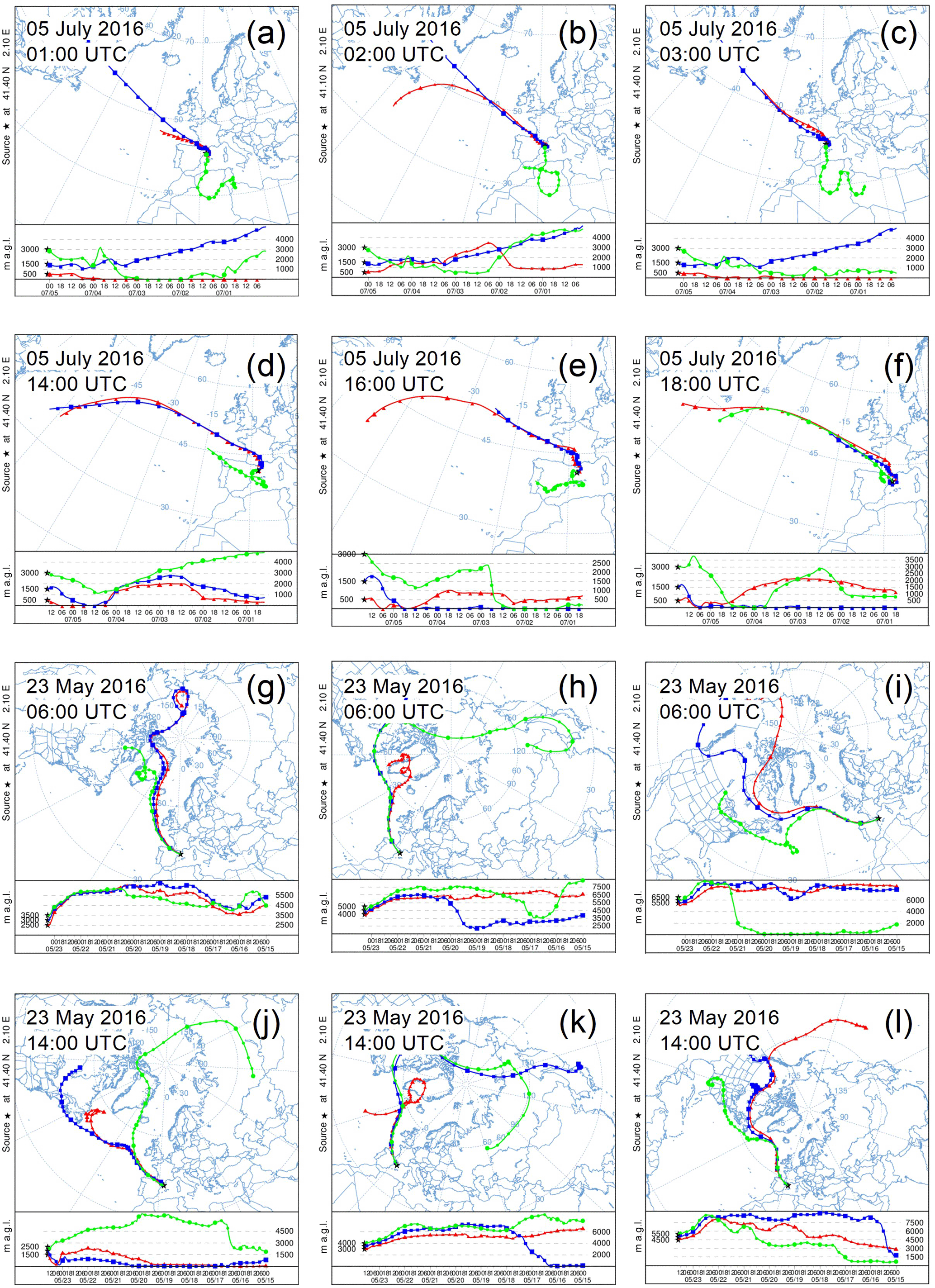
Figure 1HYSPLIT back trajectories ending at different altitudes over BCN depending on the aerosol case (only for the dust and smoke cases): (a)–(f) for dust (5 days back) on 5 July 2016 and (g)–(l) for smoke (10 days back) on 23 May 2016. Selected times of the air mass arrivals are related to those aerosol profiles that are examined in particular (as shown in Sect. 3; in particular, see Figs. 4 and 6).
The particle linear depolarization ratio δp is calculated by the procedure shown in Cairo et al. (1999) and expressed as
where R is the backscattering ratio (), βm and βp are the molecular and particle backscatter coefficients, and δmol is the molecular depolarization ratio. Optical filters of the P-MPL receiving system present a spectral band lower than 0.2 nm (Sigma Space Corporation, 2012), producing a temperature-independent δmol of 0.00363 according to Behrendt and Nakamura (2002). The particle backscatter coefficient βp is obtained by applying the Klett–Fernald (KF) algorithm (Fernald, 1984; Klett, 1985) to P () profiles obtained from P-MPL measurements in synergy with simultaneous sun-photometer measurements that provide ancillary data of the aerosol optical depth (AOD). Hence, a vertically averaged lidar ratio (LR, extinction-to-backscatter ratio, denoted by Sa) can also be estimated by using this KF iterative approach in P-MPL measurements, since the LR value varies in each iteration, reaching convergence once the relative difference between the lidar-derived height-integrated particle extinction profile τMPL () and the AERONET AOD is lower than a given convergence factor (see Córdoba-Jabonero et al., 2014 for more details of this iterative convergence method applied to specific MPL measurements). In this study, a convergence factor of 1 % is applied (relative uncertainties found for Sa are 5 %–10 %; see Table 1). AERONET V2 inversion level 1.5 data were used for all the aerosol cases due to the unavailability of the almucantar-derived data from the V3 inversion at any level and those scarce data from V2 at level 2.0. Hence, the threshold limitation of AOD > 0.4 does not apply. Both AOD and the Ångström exponent (AEx) with other AERONET parameters used in this work were also hourly averaged in order to coincide with the 1 h averaging applied to P-MPL measurements.
2.3 POLIPHON method
2.3.1 General features
The POLIPHON (POlarization-LIdar PHOtometer Networking) method was developed at the Leibniz Institute for Tropospheric Research (TROPOS, http://www.tropos.de) for application in polarization-lidar measurements in order to separate the optical properties (backscatter, extinction) of aerosol mixtures into their components with clearly different particle depolarization ratios. POLIPHON can run two ways: as a 1-step retrieval (POL-1 approach hereafter) or in 2 steps (POL-2 approach hereafter), retrieving the separation of two or three aerosol components. A complete description of the POLIPHON discrimination technique can be found in Mamouri and Ansmann (2014). In particular, the POL-1 approach has been successfully applied to separate dust from biomass-burning smoke particles (Tesche et al., 2011; Ansmann et al., 2012) and volcanic ash aerosols from other fine particles (Ansmann et al., 2012; Sicard et al., 2012). The POL-2 approach has been used for the partition of coarse and fine dust components and their discrimination from other non-dust aerosols (marine and anthropogenic pollution) (Mamouri and Ansmann, 2017).
In this work, as stated before, the separation of the optical properties of dust, smoke and pollen particles from their mixtures with other aerosols is performed by applying POLIPHON to P-MPL measurements. The POL-1 approach (2-component separation) is used for the selected smoke and pollen cases on 23 May and 23 March 2016, respectively, over BCN, in order to discriminate the smoke (SM) signature from other non-smoke (NS) aerosols, and the pollen (PL) particles from other local background aerosols (BA). The dust case observed on 5 July 2016 is examined to present the separation into three components: dust coarse (Dc), dust fine (Df) and non-dust (ND) aerosols. However, particularly for this case, instead of the POL-2 approach only, a combined version of POLIPHON using both POL-1 and POL-2 approaches (namely POL-1/2) is applied (Mamouri and Ansmann, 2017). A more detailed description of this POL-1/2 retrieval and its use in this work is shown in Sect. 2.3.2.
In general, one of the constraints of POLIPHON is that it is based on the appropriate selection of the linear depolarization ratio for each “pure” (not mixed) type of specific aerosols. Table 2 shows the particular δi values assumed for each specific (i) aerosol component. In particular, in the dust case, i=1 denotes total dust (DD) and 2 is for non-dust (ND) when using POL-1. i=1 is for dust coarse (Dc), 2 is for dust fine (Df), and 3 is for non-dust (ND) when using POL-2. In the smoke case, i=1 stands for smoke (SM) and 2 for non-smoke (NS). In the pollen case, i=1 is for pollen (PL), and 2 is for local background aerosols (BA), which are likely a mixture of small pollution particles that are mostly present in the urban environment of Barcelona city. After separation of the different aerosol components, the respective extinction coefficients are calculated by assuming LR values typical for each aerosol type: 55 sr for dust (Dc and Df components) (Mamouri and Ansmann, 2014), 70 sr for smoke plumes (Groß et al., 2013) and 50 sr for pollen particles (Sicard et al., 2016a).
The backscatter fraction for each aerosol component is presented throughout the day, as expressed in terms of the relative ratio between the specific height-integrated backscatter coefficient for each aerosol component, , and the total (sum of all the components) height-integrated particle backscatter coefficient, , i.e. the ratio (%), as calculated from the continuous 24/7 P-MPL measurements.
Table 2Aerosol cases observed over BCN on selected days. AERONET data at particular times of the event (as shown in Figs. 4, 6 and 8), including those KF-retrieved LR values (Sa), and parameters used in the POLIPHON retrieval algorithm, depending on the version applied. References for the assumed particle linear depolarization ratio for specific components δi (either i=1–3 or i=1, 2, depending on the case) are also included. Errors are shown in parentheses.

a POL-1: separation of two components; POL-2: separation of three components. b Particular δi values assumed for each specific aerosol component (i), regarded as pure aerosols: Dc, Df and ND stand for dust coarse, dust fine and non-dust particles; SM and NS stand for smoke and non-smoke aerosols; and PL and BA stand for pollen particles and local background aerosols.
2.3.2 POL1/2 approach applied to the dust case: combined POL-1 and POL-2 versions
In dust events, POL-1 is used to separate dust (DD) from non-dust (ND) aerosols. In contrast, POL-2 is a 2-step approach used to first (step 1) separate Dc particles from the total fine mode (Df + ND) (ND are assumed to be only fine aerosols as composed mostly of small pollution particles, since AODs are large enough to neglect the marine impact), and then (step 2) that fine contribution is separated into Df and ND particles (see more details in Mamouri and Ansmann, 2014). In the overall POL-2 procedure, the depolarization ratio for the total fine (Df + ND) mixture (i.e. the residual fine depolarization ratio), δDf+ND, must be either assumed or known. In our case, δDf+ND can be estimated by a combined algorithm that uses both POL-1 and POL-2 versions (POL-1/2), as also reported by Mamouri and Ansmann (2017). In particular, the statement that the backscatter coefficient profiles obtained from the POL-1 retrieval for the DD (Dc + Df) component, , is identical to the sum of the backscatter coefficient profiles for the dust coarse (Dc) and dust fine (Df) retrieved independently by the POL-2 version (i.e. and ) must be fulfilled. That is,
For that purpose, first, profiles are derived. Then, a set of both and are obtained for several δDf+ND values ranging between the specific depolarization ratios of Df particles (δDf=0.16) and ND aerosols (δND=0.05) (see Table 2). Those δDf+ND are iteratively introduced with steps of 0.01 in the POL-2 approach point-to-point along the whole profile in order to obtain an optimal δDf+ND(z) profile, which must satisfy that the two terms of the equality in Eq. (7) are equal at each z point. For instance, the minimal value obtained for the root square differences, Δ, between both terms in Eq. (7) at a given z,
is used as proxy in that iteration process. Hence, once those min{Δ} are achieved for a given δDf+ND along the whole profile, the optimal vertical δDf+ND(z) profile is determined. Moreover, since δDf+ND(z) is defined in a good approximation as
where γ(z) and (1−γ(z)) are the fraction of each Df and ND component that contributed to the total fine (Df + ND) mode mixture, this contribution of each aerosol fine component to the total fine mode can also be estimated with height and γ(z) is thus determined.
Once the profile of δDf+ND (and γ) is optimally determined, the total particle backscatter coefficient profiles β(z) can be separated into all three components (βDc, βDf and βND) for the dust case by applying the POL-2 (step 2) retrieval (see Mamouri and Ansmann, 2014, for more details). Hence, their relative contribution (i.e. the ratio, %) can also be derived.
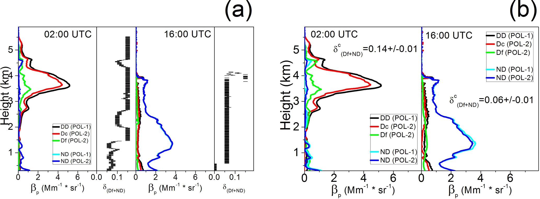
Figure 2POL-1 versus POL-2 differences in particle backscatter coefficient profiles for each component (total dust βDD and non-dust βND from POL-1; coarse βDc and fine βDf dust, being , and non-dust βND from POL-2) retrieved for the dust case on 5 July 2016 at 02:00 and 16:00 UTC by using (optimally derived) (a) a δDf+ND(z) profile and (b) a single columnar value.
For comparison, a columnar value is also calculated using the same POLIPHON procedure as described before, but the minimum of the root mean square differences, , between both terms in Eq. (7),
is used instead as the proxy applied in the iterative retrieval (n stand for the number of z points along the overall profile). For instance, Fig. 2 shows the particle backscatter coefficients profiles as obtained from either POL-1 (βDD and βND) or POL-1/2 (βDc and βDf, being , and βND) approaches twice (at 02:00 and 16:00 UTC) on 5 July 2016, using both the optimal δDf+ND(z) profile (Fig. 2a) and the columnar (Fig. 2b). Discrepancies are observed in both the dust and non-dust components by using a single columnar value instead of the optimal δDf+ND(z) profile. For comparison between Fig. 2a and b, differences are clearly found in βND at 02:00 UTC, picked at around 4.5 km in height, as derived from either POL-1 or POL-1/2, in addition to those found for βDD in comparison with βDc and βDf (particularly evident at 16:00 UTC, with βDD≪βDf between 1 and 2 km in height) (see Fig. 2b). These results highlight that the use of a height-resolved δDf+ND improves the retrieval. Indeed, the use of a single columnar (no height-resolved) (and γc) in the retrieval can be inadequate due to the plausible variability of the relative fraction of Df particles to the total fine (Df + ND) mode with height. In particular, this is corroborated by looking at the optimal height-averaged values obtained at 02:00 and 16:00 UTC are 0.12±0.04 ( %) and 0.09±0.05 ( %) in comparison with those columnar values found at 02:00 and 16:00 UTC of 0.14 (γc=82 %) and 0.06 (γc=9 %).
2.4 Extinction-to-mass concentration conversion
2.4.1 General procedure
The conversion from extinction (σ, m−1) to mass concentration (M, g m−3) is performed for each component (i) by means of the mass extinction efficiency (MEE, or mass-specific extinction coefficient) (k, m2 g−1) by using the relationship (Ansmann et al., 2012; Córdoba-Jabonero et al., 2016) at each altitude z
The effective MEE (keff, m2 g−1), linking the total aerosol extinction from all aerosol components (i.e. AOD) to the total mass concentration (TMC), is given by
where TMC = represents the total mass loading in g m−2, with the height-integrated mass concentration for each component (i.e. , with Δz the height resolution). keff is a measure of the predominant particle size; keff values lower and higher than 1.5 m2 g−1 are representative of large and small particles respectively as reported by the Optical Properties of Aerosols and Clouds database (OPAC; Hess et al., 1998). The mass contribution or fraction of each aerosol component is expressed by the relative ratio between and TMC (i.e. , in %).
Columnar MEE values can be obtained from AERONET data and the particle density (Pd, g cm−3) assumed for each aerosol component examined in this work by using the expression (Ansmann et al., 2012):
where kc,f designates the MEE for coarse and fine modes, as denoted by subscripts c and f. Similarly, VCc,f (10−12 Mm) and τc,f are the AERONET V2 L1.5 volume concentrations and extinction values for the coarse and fine modes. () are the corresponding extinction-to-volume conversion factors.
Table 3Parameters involved in the extinction-to-mass conversion for each aerosol case: the AERONET-reported and -derived mass conversion factors (cv), the assumed particle densities (Pd) and the mass extinction efficiency (k) values. For the dust case (3-component separation), i=1 (Dc), 2 (Df) and 3 (ND) and for the smoke and pollen cases (2-component separation), i=1 (SM/PL) and 2 (NS/BA). Errors are shown in parentheses.
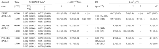
* c and f denote the particle coarse and fine modes.
Our strategy is to obtain the actual values, and then the kc,f, using typical particle densities, from AERONET sun-sky photometer observations carried out simultaneously with P-MPL observations, for as long as the separated aerosol components can be identified as being composed of pure coarse or fine particles. Table 3 shows the AERONET parameters involved in the extinction-to-mass conversion (VCc,f, τc,f) at selected times for each aerosol case together with those typical particle densities Pd for each aerosol component. In particular, Pd values assumed for each type of aerosols are 2.60 g cm−3 for dust (Ansmann et al., 2012), 1.30 g cm−3 for smoke (Reid et al., 2005) and 0.92 g cm−3 for pollen (Platanus) particles (Jackson and Lyford, 1999; Zhang et al., 2014). For the other components, the particle density is obtained from the OPAC database (Hess et al., 1998). A particle density Pd = 1.8 g cm−3 is assumed for both the ND and BA components in the dust and pollen cases, respectively, corresponding to background urban aerosols, mostly composed of fine pollution particles. For the NS component in the smoke case, a PdNS=2.0 g cm−3, as reported by OPAC for Arctic aerosols, is assumed since the NS signature is found when air masses come from the Arctic, as indicated by back-trajectory analysis (see Sect. 2.1). However, the corresponding cv and k values must be examined in more detail in the extinction-to-mass conversion procedure for each aerosol case, as explained next.
2.4.2 Dust case
As stated before, the POL-1/2 retrieval is used to separate three components for the dust case (i = Dc, Df and ND). Conversion factors are only reported for coarse- and fine-mode particles using AERONET data (Eq. 13). In this case, the coarse mode is completely composed of Dc particles (the ND component is assumed to be fine aerosols only; see Sect. 2.3). Hence, the MEE for Dc particles, kDc, is easily obtained from
with PdDc=2.6 g cm−3 for dust. However, MEE for Df particles, kDf, and ND aerosols, kND, must be determined from the MEE value obtained for the total fine (Df + ND) mode, kDf+ND, that is,
where PdDf+ND represents a weighted value of the particle density for the overall fine (Df + ND) mode. Once estimated δDf+ND, and γ (see Eq. 9), PdDf+ND can be expressed as
where PdDf and PdND are the particle densities assumed for dust (2.6 g cm−3) and non-dust aerosols (1.8 g cm−3) (Table 3). Hence, the height-integrated mass concentration for the total fine (Df + ND) mode, , can be calculated from
where kDf+ND is calculated from Eq. (15), and and are the mass concentrations for Df and ND aerosols (note that these quantities are height-integrated variables, i.e. mass loadings). In particular, can be determined by assuming a representative conversion factor cv for Df particles, since
Mamouri and Ansmann (2017) reported statistical AERONET-based extinction-to-mass conversion factors for fine-dust particles in the interval of 0.21–0.25 ( Mm. In this work, this set of values is introduced in the algorithm in order to obtain an optimal value satisfying the following condition: , being estimated from Eq. (18). At the same time, is also obtained, since
Hence, kDf and kND (and ) are calculated applying, similarly to Eqs. (13)–(15), the following expressions:
and
Otherwise, (and then, ) and . Finally, the total mass concentration TMC (i.e. mass loading, in g m−2) is obtained from
Those AERONET parameters used in the extinction-to-mass conversion with the cv and k values obtained at particular times (see Table 3) are in agreement with those reported by other authors for dust (i.e. Mamouri and Ansmann, 2014, 2017). In addition, kND values are derived between 2.52 and 2.92 m2 g−1, similarly to those reported by OPAC for urban aerosols (2.87 m2 g−1) and as assumed for the ND component in this work.
2.4.3 Smoke and pollen cases
For both cases, optical properties are separated into two aerosol components by using the POL-1 approach. Hence, mass concentrations are derived directly from Eqs. (11)–(13) of the general extinction-to-mass conversion procedure using AERONET data, satisfying that each component is composed mostly of either coarse- or fine-mode particles, as described in Sect. 2.4.1.
In particular, the smoke (SM) component is composed of fine biomass-burning particles, and the coarse mode is associated with the non-smoke (NS) component by assuming particles larger than smoke coming from the Arctic area. For instance, a m2 g−1 is derived for fine smoke particles at 06:00 UTC (see Table 3). This value is in good agreement with that reported for Canadian forest fire smoke aerosols (Ichoku and Kaufman, 2005; Reid et al., 2005). However, a rather lower MEE value is obtained for the coarse-mode NS particles ( m2 g−1) at the same time. In the pollen case, PL particles are predominantly large particles in comparison with the fine (and less depolarizing) component corresponding to local background aerosols (BA), which are assumed to be composed of small pollution particles of urban origin (marine contribution is neglected, as stated in Sect. 2). For instance, a m2 g−1 is obtained for pollen particles at 15:00 UTC, when the pollination event is enhanced, as described later in Sect. 3.3.
Table 3 shows the derived MEE values (k, m2 g−1) at selected times by using the corresponding cv factors and the assumed particle densities (Pd, g cm−3) for each component. Particular similarities and discrepancies found from those assumptions will be discussed in more detail in Sect. 3.
Table 4Height-integrated mass concentration (, i.e. mass loading, g m−2) for each component and the total mass concentration (TMC) indicated for two times for each aerosol case. Errors are shown in parentheses.
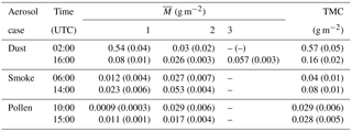

Figure 3Dust event on 5 July 2016. Evolution of the relative contribution (a) (%) and (b) (%) (the bar over the variable are removed in the figure for clarity) for each aerosol component throughout the day: Dc (red bars), Df (green bars) and ND (blue bars), which denote dust coarse, dust fine and non-dust aerosols. In (a) (right axis) AERONET hourly averaged AOD and AEx (white and black–white stars, respectively) and KF-derived Sa (lidar ratio, sr; square symbols) values are reported; in (b) (right axis) TMC (total mass loading, g m−2; open circles) is also included. Black arrows on the time axis indicate selected times for those vertical profiles shown in Fig. 4.
3.1 Dust case
A dust event occurred over BCN on 5 July 2016, which was mostly intense before 12:00 UTC as confirmed by AERONET data with moderate AOD and AEx < 0.5 values together with HYSPLIT back-trajectory analysis (Sect. 2.1). The separation into three components (Dc, Df and ND) of dust mixtures using the synergy of hourly averaged P-MPL measurements and POL-1/2 retrieval was performed throughout the day. Prior to using POL-1/2, vertical profiles of the total particle backscatter coefficient (βp), as derived from the KF algorithm (if the KF retrieval is feasible, estimated LR values are discussed later), and the linear particle depolarization ratio (δp) are obtained throughout the day. Then, the corresponding vertical profiles of the backscatter coefficients for each specific component (βi, i = Dc, Df, ND) were retrieved by using POL-1/2 (Sect. 2.3.2). The three specific depolarization ratios selected for each pure aerosol component (δi, i = Dc, Df, ND), required for the POL-1/2 retrieval, are shown in Table 2. As mentioned before, height-integrated values of all these backscatter coefficient profiles (, and the three for each component) are calculated over 24 h (if the KF retrieval is feasible) to obtain the daily temporal evolution of the optical contribution for each aerosol component in terms of their specific relative ratio (in %). Regarding the height-integrated mass concentration (, i = Dc, Df, ND; Sect. 2.4), the daily evolution of the specific mass contribution ratio (i.e. the relative ratio , in %) is also calculated for each aerosol component (note that height-integrated mass concentrations represent the mass loading, expressed in g m−2). For simplicity, the same notation is used for mass concentration and mass loading.
Figure 3 shows the daily evolution of the specific (a) optical and (b) mass relative contributions for each aerosol component throughout the day. A high loading of large particles with peaks of 78 % for βDc and 98 % for MDc was obtained in the time interval before 12:00 UTC. These peaks drop to minimums of 9 % and 43 % after that time. Here, the optical contribution of the total dust (Dc+Df) varies between 17 % and 46 %, while the mass contribution ratio varies between 56 % and 98 %. In terms of mean TMC (dust loading), values of 0.6±0.1 and 0.2±0.1 g m−2 are estimated at those time intervals before and after 12:00 UTC. The last one represents a TMC of 34 % with respect to that found in the previous period of the day. Specific and TMC at given times are shown in Table 4. Therefore, two differentiated dust scenarios with an intense and weak dust impact are clearly observed throughout the day.
These results are related to the mean MEE values found for dust particles, m2 g−1 and m2 g−1, as obtained for Dc and Df particles. These quantities are within and close to the range of values representative of coarse- and fine-dominated dust particles as reported by the OPAC database (Hess et al., 1998): 0.16–0.97 m2 g−1 (dust coarse) and 2.3–3.1 m2 g−1 (dust fine). Higher MEE values are obtained for the ND component ( m2 g−1, in daily average), indicating much smaller particles, and are close to the value of 2.87 m2 g−1 reported by OPAC (Hess et al., 1998) for urban aerosols (note that fine polluted aerosols with urban origin were assumed for the ND component). For comparison, the corresponding mean conversion factors cv obtained for Dc and Df particles are Mm and Mm, which are in good agreement with other reported values (i.e. Mamouri and Ansmann, 2017).
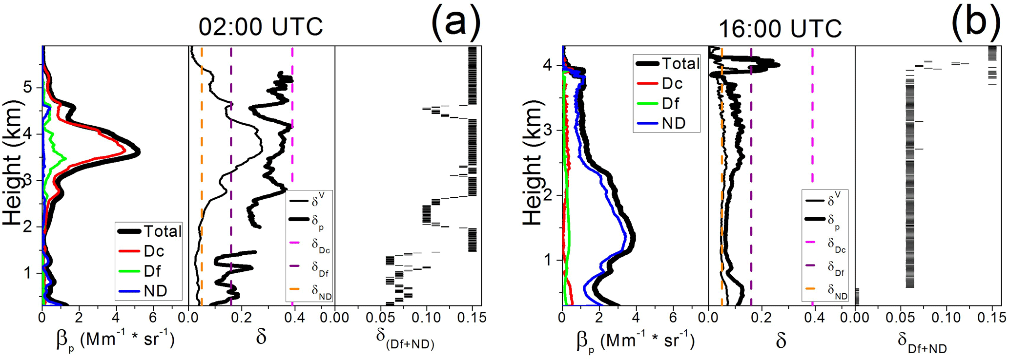
Figure 4Dust event on 5 July 2016. Vertical profiles of the particle backscatter coefficients (total and for each specific component; left panels), the linear depolarization ratios (volume δV and particle δp; centre panels) and the estimated depolarization ratio for the fine (Df + ND) mode (δDf+ND; right panels) at two time intervals, illustrating the different aerosol scenarios observed throughout the day: (a) at 02:00 UTC (high dust incidence) and (b) at 16:00 UTC (low dust incidence). Specific depolarization ratios selected for each pure aerosol component are also shown by vertical dashed lines (see legend) in the centre panels.
AERONET AOD and AEx values provided throughout the day also confirm these results (night-time data are assumed equal to the first and last daytime values in each case; see Fig. 3a). In particular, AEx is close to 0.5 (coarse particle predominance) and higher than 1.5 (fine particle prevalence) before and after 12:00 UTC. Regarding LR values as derived from the KF algorithm (Fig. 3a, right axis), a daily mean sr is obtained. No significant differences are found between LR values obtained for those intense and weak dust periods of the day and only a certain variability is observed throughout the day as modulated by the dust loading, as expected.
In order to illustrate the vertical distribution of dust particles, Fig. 4 shows an example in terms of the profiles of both the particle backscatter coefficients (total βp, and βDc, βDf and βND, left panels) and the linear depolarization ratios (volume δV and particle δp, right panels) of both aerosol scenarios: (1) when the dust event presents a high incidence, as occurred for instance at 02:00 UTC (Fig. 4a); and (2) after the dust particles have been almost completely removed (i.e. situation observed at 16:00 UTC; see Fig. 4b). These scenarios are also indicated in Fig. 3 by black arrows. An enhanced dust impact is observed in Fig. 4a (02:00 UTC) due to a high quantity of Dc particles confined in a layer located between 2 and 5 km in height (red line in Fig. 4a). Contrarily, Fig. 4b (16:00 UTC) shows a rather weaker dust incidence from the ground up to 4 km, mostly due to a low loading of both Dc and Df particles (red and green lines in Fig. 4b). Indeed, according to HYSPLIT back trajectories (Sect. 2.1), no Saharan origin of air masses is observed after 12:00 UTC (see Fig. 1d and e).
AERONET AOD and AEx and KF-derived LR values for those different dust scenarios are also included in Table 2. In particular, a sr is retrieved at 02:00 UTC that is within the typical LR range determined for dust. Meanwhile a lower value ( sr) is found at 16:00 UTC, when a rather weaker dust incidence occurs. Moreover, δp shows values close to the linear particle depolarization ratio for pure Dc particles (δDc=0.39) for the first aerosol scenario (Fig. 4a, centre panels) and values slightly lower than 0.16 (δDf for pure fine dust particles) for the second one (Fig. 4b, centre panels). In addition, the δDf+ND profiles for those times are also shown in Fig. 4 (right panels) in order to examine the corresponding variability of the Df contribution to the particle fine mode with height: δDf+ND is greater than 0.10, indicating that the Df fraction within the fine mode is larger than 45.5 % at altitudes higher than 1.5 and around 4.0 km for those two dust situations (Fig. 4a and b), in correspondence with the backscatter profiles; otherwise, the Df fraction is reduced (<40 %) at lower heights. In these two particular cases (Fig. 4), the derived MEE values are close to the typical ranges for Dc (kDc: 0.5–0.6) and Df (kDf: 1.5–2.0) aerosols (see Table 3).
3.2 Smoke case
Smoke plumes were observed over BCN station on 23 May 2016. The two principal areas from which air masses arrive are North America and the Arctic, as reported by HYSPLIT back-trajectory analysis (see Fig. 1g–l panels). The smoke origin is likely from forest fires in North America (as stated in Sect. 2.1). Hence, the smoke case is examined as a mixture of two components: fine biomass-burning particles (SM for smoke) from Canada and USA fires, and another particle type larger than smoke coming from the Arctic region (hereafter referred to as non-smoke aerosols, NS). Their vertical separation is achieved using a POL-1 retrieval (2-component separation), as described in Sect. 2.3 and 2.4. Both the particular backscatter coefficients and mass concentrations are retrieved for each component. In particular, the arrival of smoke plumes over BCN is mostly at altitudes above the boundary layer (BL); hence, this case is focused only on those tropospheric features above the BL, thus disregarding aerosols from other plausible local background BL sources.
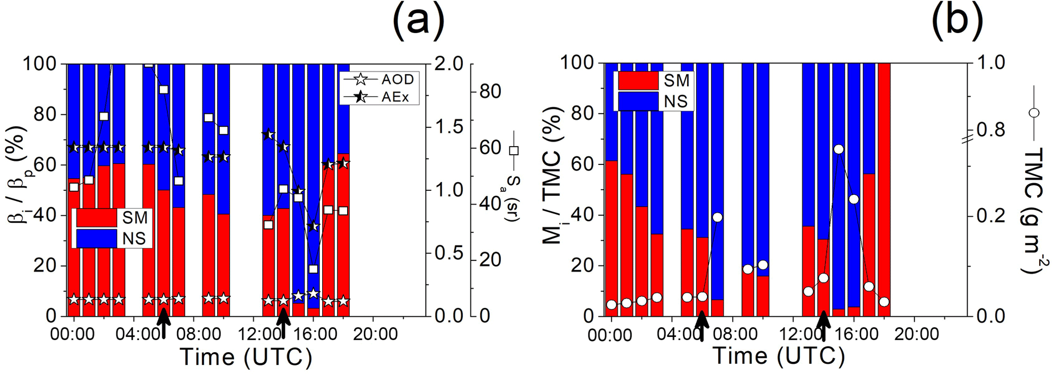
Figure 5The same as Fig. 3 but for the smoke case on 23 May 2016: SM (red bars) and NS (blue bars) denote smoke and non-smoke components. Black arrows on the time axis indicate selected times for vertical profiles shown in Fig. 6.
Like for the dust case, Fig. 5 shows the relative fractions of each SM and NS component in terms of the backscatter coefficient and the mass concentration throughout the day. Those k values, together with the cv factors at selected times, are shown in Table 3 along with the assumed Pd values: 1.30 g m−3 for SM and 2.0 g m−3 for NS aerosols (see Sect. 2.4). Since values of δp higher than 0.1 are found at given altitudes throughout the day, a high-limit value of the particle linear depolarization ratio for smoke, δSM of 0.15, is assumed. This rather high δSM value is typical for smoke particles mixed with dust (Tesche et al., 2011; Groß et al., 2013), as one would expect δSM<0.10 for pure biomass-burning particles (Müller et al., 2005; Groß et al., 2013). In addition, AERONET AEx varies between 1.25 and 1.55 before 12:00 UTC (see Fig. 5a), indicating rather moderate AEx values compared to higher fresh smoke values (∼2.00), as also measured by Sicard et al. (2011) in Barcelona. Hence, the value of δSM=0.15 reflects a mixing state of biomass-burning particles but not necessarily with dust. For the other, less depolarizing, NS component, a δNS=0.05 is applied. Those particle linear depolarization ratio values assumed for SM and NS are shown in Table 2.
In general, smoke particles are detected almost throughout the whole day, representing approximately 40 %–60 % of the total height-integrated aerosol backscatter. However, a sharp decrease from those values to around 4 % is observed at 15:00 and 16:00 UTC, which coincides with the 47 % decrease found for AEx (see Fig. 5a). Since lower AEx values are usually associated with the predominance of large particles and/or the decrease in the fine mode, these results are in agreement with the observed reduction of fine biomass-burning particles in the same time interval. At those same times, the TMC reaches high values (0.26±0.06 g m−2, in average) with respect to the daily mean TMC background of 0.05±0.03 g m−2. This is likely due to the major contribution of larger NS aerosols; meanwhile fine SM particles represent only a 3 %–7 % of TMC at the same times. In particular, the daily mean is 0.017±0.008 g m−2, representing 2.7 % of the mean TMC found for the dust case. Regarding KF-derived LR values (see Fig. 5a, right axis), a daily mean sr is obtained. That value is lower compared to typical LR of 70 sr for smoke (i.e. Groß et al., 2013, and references therein), which together with the large relative deviation (42 %) indicates a high aerosol variability throughout the day as expected due to the singular arrival of air masses in height and time, and hence the particular vertical aerosol mixing found with the smoke particles.
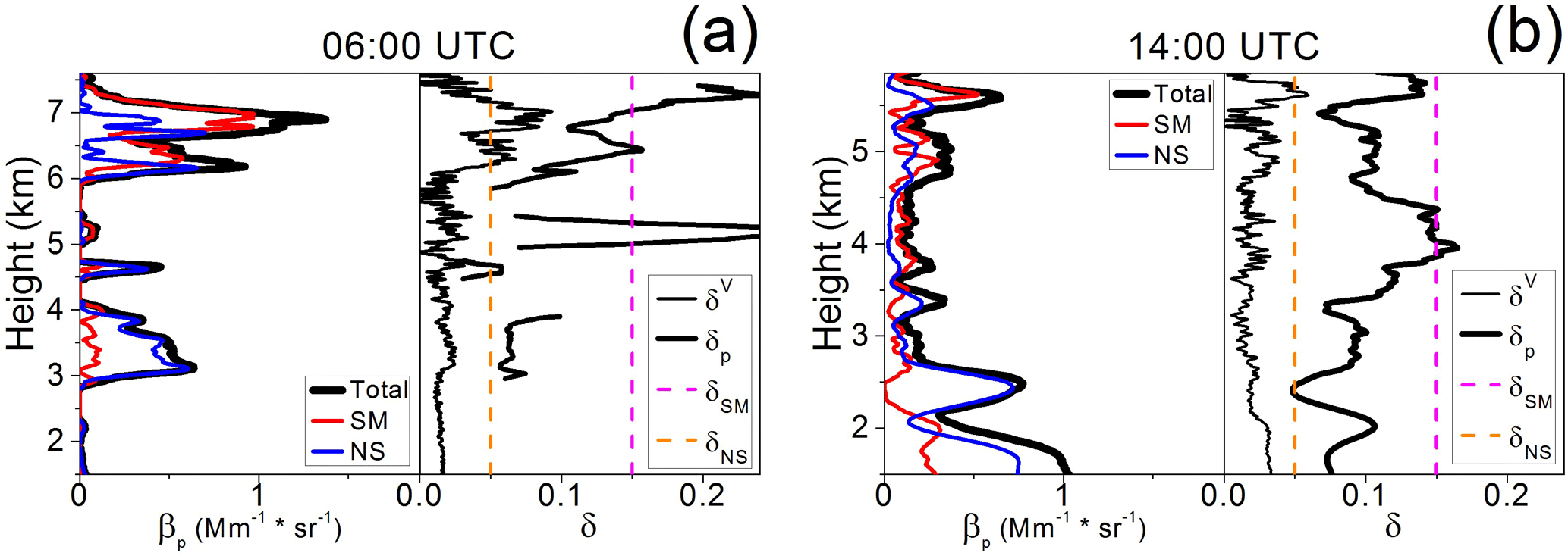
Figure 6The same as Fig. 4 but for the smoke event on 23 May 2016 at (a) 06:00 UTC, and (b) 14:00 UTC. Specific depolarization ratios selected for each smoke aerosol component are also shown by vertical dashed lines (see legend for details).
Regarding the vertical structure, Fig. 6 shows examples of two different aerosol scenarios observed on 23 May 2016 (smoke case): (1) a well-defined smoke layer is observed, for instance, between 6 and 7.5 km in height with a certain mixing with NS aerosols at 06:00 UTC (see Fig. 6a, red line); and (2) the smoke signature can be detected as highly mixed with NS aerosols along the atmospheric profile (i.e. situation observed at 14:00 UTC; see Fig. 6b). Both these scenarios are also indicated in Fig. 5 with black arrows. Indeed, the mean Sa values of 70±19 and 35±9 sr found before and after 12:00 UTC reflect that the smoke signature detected during the first of those time periods of the day presents a lower mixing with other aerosols than that observed later. Additionally, on average, the mean height-integrated mass concentration for smoke is also obtained in those two scenarios: and 0.022±0.009 g m−2 are found for those time intervals. Those values represent 2.2 % and 3.4 % of the TMC found for the intense dust period. Figure 6a clearly shows a smoke layer between 6 and 7.5 km in height, also mixed with a certain NS contribution, exhibiting δp values of 0.15 and higher. In addition, a smaller SM layer of about 300 m thickness is also found below, at around 5.2 km in height, with rather higher δp than 0.15, and another layer is observed between 3 and 4 km in height corresponding to the presence of NS aerosols with a δp slightly higher than 0.05. The fraction of smoke particles is around 50 % of total backscatter (see Fig. 5a) with a height-integrated mass concentration for smoke g m−2, representing 2 % of the mean TMC during the intense dust event (see Table 4).
Later in the day at 14:00 UTC, both SM and NS particles are found along all the profile, with δp values close to 0.15, mainly between 4.0 and 4.5 km in height. In addition, a single NS layer is also clearly observed, peaking at 2.5 km in height, with δp values decreasing to 0.05 (see Fig. 6b). These results agree with the δp value selected for NS aerosols (δNS=0.05; see Table 2). At this time, a g m−2 is obtained, being 4 % of the mean TMC for the intense dust episode. Particular LR values for those times shown in Fig. 6 are also included in Table 2: sr is retrieved at 06:00 UTC, which is within the typical LR range determined for smoke, while a lower LR ( sr) is found at 14:00 UTC, as expected. Particular MEE values derived for smoke particles, and 1.9±0.4 m2 g−1, are obtained at 06:00 and 14:00 UTC. These results would indicate that smoke plumes detected in the first scenario are predominantly composed of relatively pure fine biomass-burning particles, with similar MEE values to those reported for Canadian boreal forest fire aged smoke particles (Ichoku and Kaufman, 2005; Reid et al., 2005). However, those observed in the second one would represent a mixed state of smoke particles with an enhanced coarse mode, thus decreasing their MEE. All those values are shown in Tables 3 and 4.
These results are corroborated by a more detailed analysis of the back trajectories ending over BCN on 23 May 2016 (selected heights and times of their arrival are shown in Fig. 1). In particular, air masses arriving at 06:00 UTC carry smoke particles from Canada and USA fires at altitudes higher than around 4500 m a.s.l. (see Fig. 1h and i), while Arctic air masses arrive at lower heights (see Fig. 1g). Later on, a smoke signature observed at 14:00 UTC is distributed from altitudes higher than around 3000 m a.s.l. (Fig. 1k and l), and the NS layer identified at around 2500 m height (see Fig. 6b) actually corresponds to air masses from the Arctic (see Fig. 1j).
3.3 Pollen case
The pollination period (i.e. the enhanced formation/presence of pollen particles) in Barcelona is from local sources predominately occurring in March from more abundant species, such as the Pinus and Platanus trees (Sicard et al., 2016a). In this case, a pollen episode occurred on 23 March 2016, corresponding to a high pollination event observed over BCN (Belmonte, 2016). As for the smoke case, a POL-1 retrieval is used to separate pollen (PL) particles from background (BA) aerosols. These BA are supposed to be mostly composed of fine urban pollution particles, and their exact origin, whether they are local or not, is not relevant since they do not depolarize and cannot be mistaken for highly depolarizing pollen particles. This is also the reason that HYSPLIT back trajectories were not calculated. Particle linear depolarization ratios for pure PL, δPL=0.40, and BA, δBA=0.05, aerosols are shown in Table 2, and k (and cv) values are shown in Table 3. The relative fractions of each aerosol component in terms of the backscatter coefficient and the mass concentration are also calculated throughout the day.

Figure 7The same as Fig. 3 but for the pollen event that occurred on 23 March 2016: PL (red bars) and BA (blue bars) denote pollen and local background aerosol components. Black arrows on the time axis indicate selected times for those vertical profiles shown in Fig. 8.
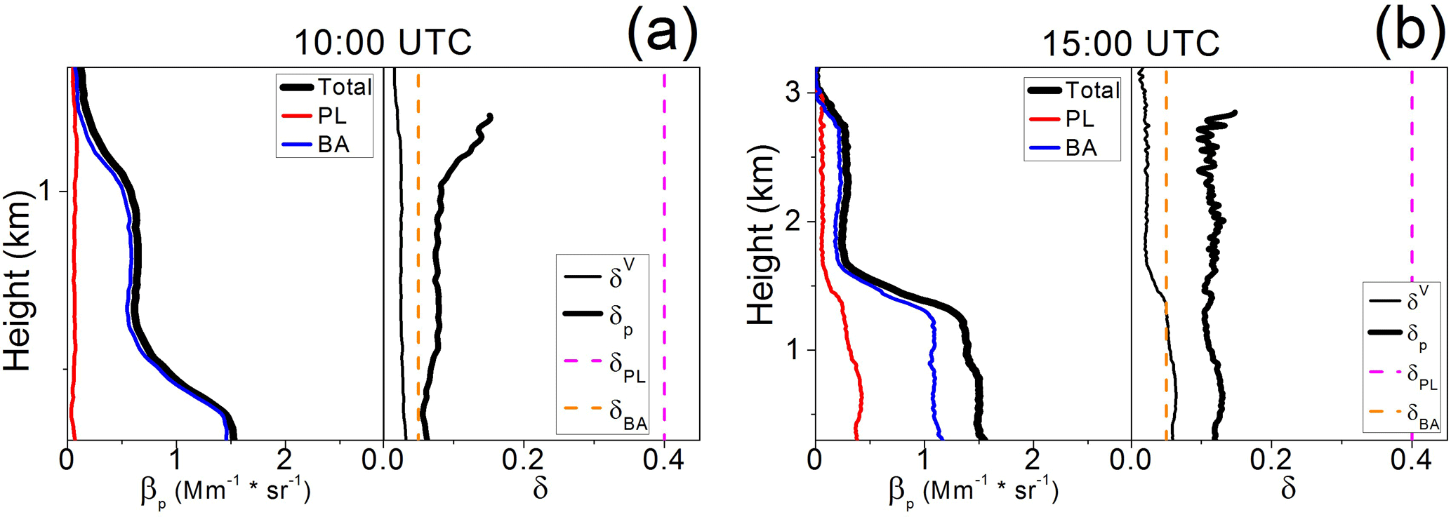
Figure 8The same as Fig. 4 but for the pollen event on 23 March 2016 at (a) 10:00 UTC (no PL detection) and (b) 15:00 UTC (enhanced PL occurrence). Specific depolarization ratios selected for each pure aerosol component are also shown by vertical dashed lines (see legend for details).
Pollen signature is clearly observed from 10:00 UTC, as shown in Fig. 7 by the increase in their relative fraction , with a maximum around 30 % between 12:00 and 16:00 UTC. The coincident increase in AEx (see Fig. 7a) is probably associated with the formation of local urban aerosols, which are much smaller than pollen grains. This hypothesis suggests that local urban aerosols dominate the columnar-averaged optical properties. A mean value of sr is obtained during the pollen occurrence, while sr is found for the no pollen detection period. The Sa value for pollen is close to that considered in other works (Sicard et al., 2016a). The fraction of the height-integrated mass concentration for pollen with respect to the TMC reaches a maximum of around 40 % at 15:00 UTC. In addition, the TMC evolution is fairly constant with a daily averaged TMC of 0.029±0.003 g m−2 and a mean of g m−2 (i.e. 25 % of TMC) in the 12:00–23:00 UTC interval. For comparison, these TMC levels represent only 1.1 % of the dust TMC during their higher dust incidence, as discussed in Sect. 3.1.
Regarding the MEE derived for pollen particles, a mean m2 g−1 is obtained. Sicard et al. (2016a) estimated a kPL=3.2 m2 g−1 considering an effective radius size of 24 µm for the pollen grains registered during a pollination episode in March 2015 (data not shown). Hence, the kPL value found in this work may be in agreement with the estimated value if pollen particles detected in our case are larger than those observed by Sicard et al. (2016a), as MEE decreases as particle size increases.
In order to display the vertical distribution for this case, profiles of the particle backscatter coefficients and both the volume and particle linear depolarization ratios are shown in Fig. 8 (see legend inside). For instance, the vertical distribution is shown at 10:00 UTC when no pollen particles are significantly detected (Fig. 8a), with low δp values close to 0.05 from the surface up to around 1 km and slightly increasing from that altitude up. This is likely due to uplifted particles. In comparison, the situation occurred later in the day (i.e. that observed at 15:00 UTC, Fig. 8b), the amount of pollen is clearly enhanced: δp increases, reaching higher values between 0.10 and 0.15, and pollen particles are mostly confined up to 1.5 km from the surface. These two scenarios are also indicated in Fig. 7 with black arrows. The corresponding mass loading for pollen at this time is 0.011±0.003 g m−2 (see Table 4).
The synergetic use of the POLIPHON (POlarization-LIdar PHOtometer Networking) retrieval with the MPLNET (Micro-Pulse Lidar NETwork)/P-MPL (polarized MPL) measurements is introduced for the first time in order to separate dust (both coarse Dc, and fine Df, modes) and biomass-burning smoke (SM) particles from their mixtures with other aerosols (namely, non-dust ND, and non-smoke NS aerosols). In addition, a case study of pollen (PL) mixed with local urban background aerosols (BA) is also examined. In all cases, the particle linear depolarization ratio for each pure aerosol component is a relevant constraint in POLIPHON retrievals. The separation of aerosol mixtures into their particle components is performed for different depolarizing particles. In particular, typical linear depolarization ratios found in the literature are assumed for each pure aerosol component: 0.39, 0.16 and 0.05 for Dc, Df and ND; 0.15 and 0.05 for SM and NS; and 0.40 and 0.05 for PL and BA.
In this work, a reasonable performance is achieved by obtaining the relative optical and mass contributions of each aerosol component throughout the day as based on P-MPL continuous 24/7 observations carried out in Barcelona (NE Spain). Three case studies observed on 5 July, 23 May and 23 March 2016 are examined respectively for dust, smoke and pollen occurrences. In particular, the POLIPHON 1-step version (POL-1: separation into two components) is applied for the smoke and pollen cases. In order to illustrate the 3-component separation for the dust case, a combined algorithm using both the POLIPHON 1-step (POL-1) and 2-step (POL-2) versions (namely POL-1/2) is described in more detail. In addition, both the vertical and columnar particle depolarization ratios for the total fine (Df + ND) mode, δDf+ND, and correspondingly both the vertical and columnar fraction of Df particles to the total fine (Df + ND) mode, are also estimated using the POL-1/2 retrieval (the a priori assumption of those variables is thus avoided). Minimal differences in the particle backscatter coefficient, β, for each dust and non-dust component are obtained from either POL-1 or POL-1/2 approaches, as long as a vertical depolarization ratio for the total fine (Df + ND) mode δDf+ND(z) is regarded. Otherwise, the use of a single columnar that is not height resolved, , is inadequate due to the plausible Df variability, with respect to the total fine mode with height.
The extinction-to-mass conversion procedure is described in terms of the mass extinction efficiency (MEE: k, m2 g−1), a parameter associated with the size of the particles. The MEE is estimated for each aerosol component by using the corresponding conversion factors as calculated from AERONET data (volume concentrations and extinctions for the coarse and fine modes), as reported simultaneously with P-MPL measurements, and the particles densities assumed for each type of aerosol. In addition, the effective MEE (keff, a measure of the predominant size of those aerosol mixtures) is also retrieved for each aerosol event. Hence, height-integrated mass concentrations (i.e. mass loadings, g m−2) are obtained throughout the day for each component. In general, the daily evolution of their relative optical and mass contributions, with respect to the height-integrated total backscatter coefficient and total mass concentration (total mass loading) for each aerosol case, is also derived. Due to the variation of the aerosol situation observed for each case study throughout the day, different aerosol scenarios can be present, and hence their vertical distributions are examined.
In the dust case on 5 July 2016, a Saharan dust intrusion arrives at BCN during the first part of the day (before 12:00 UTC). Meanwhile a weak dust incidence is observed later on, as also confirmed by AERONET data and a HYSPLIT back-trajectory analysis. This is due to the predominance of large particles (Dc component) during this intense dust period of the day. In terms of mean dust mass loading, values of TMC = 0.6±0.1 and 0.2±0.1 g m−2 are obtained at time intervals before and after 12:00 UTC. This last value just represents a mass loading of 34 % with respect to that found before. In addition, mean MEE values of m2 g−1 and m2 g−1 are obtained for Dc and Df particles. These quantities are within and close to the range of values representative of coarse- and fine-dominated dust particles. AERONET AOD and AEx values reported throughout the day confirm these results. In particular, AEx is close to 0.5 (predominance of coarse particles) and higher than 1.5 (fine particles prevalence) before and after 12:00 UTC. A mean KF-derived lidar ratio sr is obtained with no significant differences for those two time periods of the day.
Regarding particular aerosol scenarios, a sr is retrieved at 02:00 UTC (within the typical range of lidar ratios defined for dust); meanwhile a lower value ( sr) is found at 16:00 UTC when a rather weaker dust incidence occurs. Moreover, δp shows values close to the particle linear depolarization ratio for pure Dc particles (0.39) during the intense dust scenario, and lower than 0.16 (typical for pure fine dust particles) for the weak one, highlighting the prevalence of ND aerosols. In addition, the particle depolarization ratio for the total fine (Df + ND) mode is greater than 0.10; that is, the relative Df fraction within the total fine mode is larger than 45.5 %, at altitudes higher than 1.5 and around 4.0 km for those two particular dust situations. The derived MEE values are typical for Dc (kDc: 0.5–0.6) and Df (kDc: 1.5–2.0) aerosols in those two particular cases.
For a smoke case, air masses arriving over Barcelona (BCN) on 23 May 2016 come from two areas, North America and the Arctic, as reported by HYSPLIT back-trajectory analysis. Fine biomass-burning particles originated from fires in Canada and the USA, which were likely mixed with other aerosols larger than smoke from the Arctic region (non-smoke aerosols, NS). In general, both SM and NS particles were found along all the profile; δp values are higher than 0.10 and close to 0.15 when SM particles were mostly detected. Fine smoke particles are observed during almost all the day, representing approximately 40 %–60 % of the total height-integrated aerosol backscatter coefficient. The mean mass loading for smoke is g m−2, representing 2.7 % of the mean TMC found for the dust case. However, individual decreases in the relative smoke fractions of both the backscatter coefficient and mass concentration are also observed throughout the day, also coinciding in time with AEx decreases (as associated with a predominance of coarse particles or reduction of fine ones).
Regarding the vertical structure, two aerosol scenarios are observed throughout the day: the smoke signature is detected at defined layers in the morning, while a vertical SM distribution mixed with a layered NS structure is observed later on. Mean LR values of and 35±9 sr are found before and after 12:00 UTC that day, showing a lower smoke mixing for the first time interval. In addition, the mean mass loadings for smoke as obtained in those two different scenarios are and 0.022±0.009 g m−2 (i.e. 2.2 % and 3.4 % of the TMC found for the intense dust period). This is likely due to the singular arrival of air masses in height and time, and hence the particular vertical aerosol mixing found together with the smoke particles over BCN. Corresponding MEE values derived for smoke particles in those two scenarios are and 1.9±0.4 m2 g−1 indicating that smoke plumes detected in the first scenario are predominantly composed of pure fine biomass-burning particles, unlike the second one, which has a mixed state of smoke particles with an enhanced coarse mode.
In the pollen case on 23 March 2016, the PL signature is clearly observed from 10:00 UTC, when the relative fraction of the height-integrated backscatter coefficient for pollen enhances, reaching a maximum around 30 % between 12:00 and 16:00 UTC, and δp increases with values between 0.10 and 0.15 from the surface up to around 1.5 km. A mean LR of sr is obtained during the pollen occurrence period. This value is close to that considered by other authors. The relative fraction of mass loading for pollen reaches a maximum of around 40 % at 15:00 UTC and is g m−2 (i.e. 1.7 % of that for dust during their higher incidence). In addition, the mean MEE derived for pollen particles is m2 g−1, representing an intermediate value between those reported for Df particles ( m2 g−1) and for smaller local background urban polluted aerosols ( m2 g−1). However, the kPL can reach higher or lower values depending on prevalently smaller or larger pollen grain sizes.
In summary, the vertical separation of aerosol mixtures into their components is achieved using the POLIPHON retrieval in synergy with continuous 24/7 P-MPL measurements together with AERONET data. The methodology, including the extinction-to-mass conversion procedure, is described and applied to several aerosol mixture case studies. Therefore, vertical optical and mass features are obtained on a daily basis for different climate-relevant aerosols: dust, smoke and pollen particles. It should be noted that the method can be relatively easily applicable to other P-MPLs also within the worldwide NASA Micro-Pulse Lidar Network (MPLNET), since all those systems present the same instrumental and operating configuration. Hence, the aerosol discrimination can be extended on a global scale. In addition, it can also be adapted to space-borne lidars with an equivalent configuration (elastic with a depolarization-sensitive channel), such as the ongoing CALIOP/CALIPSO and the forthcoming ATLID/EarthCARE (future ESA mission to be launched in 2019).
Data sets and source codes underlying this work can be requested via email to the corresponding author. The Barcelona P-MPL data are available upon request via email (msicard@tsc.upc.edu). AERONET data are downloaded from the AERONET web page (AERONET, 2017). Backward trajectories analysis has been supported by air mass transport computation with the NOAA (National Oceanic and Atmospheric Administration) HYSPLIT (HYbrid Single-Particle Lagrangian Integrated Trajectory) model (HYSPLIT, 2017) using GDAS meteorological data (Stein et al., 2015; Rolph et al., 2017).
Table A1List of acronyms.
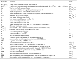
a i denotes the aerosol component: dust coarse (Dc), dust fine (Df), non-dust (ND), smoke (SM), non-smoke (NS), pollen (PL), background aerosols (BA); b x denotes the particle size mode: coarse (c), fine (f).
The authors declare that they have no conflict of interest.
This work is supported by the Spanish Ministerio de Economía y
Competitividad (MINECO) under grant CGL2014-55230-R (AVATAR project) and the
ACTRIS-2 (Aerosols, Clouds, and Trace Gases Research Infrastructure Network)
Research Infrastructure Project funded by the European Union's Horizon 2020
research and innovation programme (grant agreement no. 654109). Lidar
measurements in Barcelona were also supported by the Spanish MINECO (project
TEC2015-63832-P) and EFRD (European Fund for Regional Development); by the
Department of Economy and Knowledge of the Catalan autonomous government
(grant 2014 SGR 583); and the Unidad de Excelencia Maria de Maeztu
(project MDM-2016-0600) financed by the Spanish Agencia Estatal de Investigación.
The MPLNET project is funded by the NASA Radiation Sciences Program and
Earth Observing System. The authors gratefully acknowledge the NOAA Air
Resources Laboratory (ARL) for the provision of the HYSPLIT transport and
dispersion model and/or READY website (http://www.ready.noaa.gov, November 2017) used in
this publication. Carmen Córdoba-Jabonero thanks the Ministerio de Educación, Cultura y
Deporte (MECD) support under grant PRX15/00375 for the 3-month research stay
at TROPOS (Germany); and Ana del Águila thanks the MINECO support (Programa de
Ayudas a la Promoción del Empleo Joven e Implantación de la
Garantía Juvenil en i + D + i) under grant PEJ-2014-A-52129.
Edited by: Andrew Sayer
Reviewed by: four anonymous referees
AERONET: AERONET aerosol data base, available at: http://aeronet.gsfc.nasa.gov/, last access: 17 November 2017.
Ansmann, A., Tesche M., Seifert P., Groß, S., Freudenthaler, V., Apituley, A., Wilson, K. M., Serikov, I., Linné , H., Heinold, B., Hiebsch, A., Schnell, F., Schmidt, J., Mattis, I., Wandinger, U., and Wiegner, M.: Ash and fine mode particle mass profiles from EARLINET-AERONET observations over central Europe after the eruptions of the Eyjafjallajökull volcano in 2010, J. Geophys. Res., 116, D00U02, https://doi.org/10.1029/2010JD015567, 2011.
Ansmann, A., Seifert, P., Tesche, M., and Wandinger, U.: Profiling of fine and coarse particle mass: case studies of Saharan dust and Eyjafjallajökull/Grimsvötn volcanic plumes, Atmos. Chem. Phys., 12, 9399–9415, https://doi.org/10.5194/acp-12-9399-2012, 2012.
Behrendt, A. and Nakamura, T.: Calculation of the calibration constant of polarization lidar and its dependency on atmospheric temperature, Optics Express, 10, 805–817, 2002.
Belmonte, J.: Personal Communication, Institut de Ciència i Tecnologia Ambientals, Universitat Autònoma de Barcelona, Barcelona, Spain, 2016.
Böckmann, C., Mironova, I., Müller, D., Schneidenbach, L., and Nessler, R: Microphysical aerosol parameters from multiwavelength lidar, J. Opt. Soc. Am. A, 22, 518–528, 2005.
Boucher, O., Randall, D., Artaxo, P., Bretherton, C., Feingold, G., Forster, P., Kerminen, V.-M., Kondo, Y., Liao, H., Lohmann, U., Rasch, P., Satheesh, S. K., Sherwood, S., Stevens, B., and Zhang, X. Y.: Clouds and Aerosols, in: Climate Change 2013: The Physical Science Basis, Contribution of Working Group I to the Fifth Assessment Report of the Intergovernmental Panel on Climate Change, edited by: Stocker, T. F., Qin, D., Plattner, G.-K., Tignor, M., Allen, S. K., Boschung, J., Nauels, A., Xia, Y., Bex, V., and Midgley, P. M., Cambridge University Press, Cambridge, UK and New York, NY, USA, 2013.
Burton, S. P., Ferrare, R. A., Hostetler, C. A., Hair, J. W., Rogers, R. R., Obland, M. D., Butler, C. F., Cook, A. L., Harper, D. B., and Froyd, K. D.: Aerosol classification using airborne High Spectral Resolution Lidar measurements – methodology and examples, Atmos. Meas. Tech., 5, 73–98, https://doi.org/10.5194/amt-5-73-2012, 2012.
Burton, S. P., Vaughan, M. A., Ferrare, R. A., and Hostetler, C. A.: Separating mixtures of aerosol types in airborne High Spectral Resolution Lidar data, Atmos. Meas. Tech., 7, 419–436, https://doi.org/10.5194/amt-7-419-2014, 2014.
Cairo, F., Di Donfrancesco, G., Adriani, A., Pulvirenti, L., and Fierli, F.: Comparison of various depolarization parameters measured by lidar, Appl. Optics, 38, 4425–4432, 1999.
Campbell, J. R., Hlavka, D. L., Welton, E. J., Flynn, C. J., Turner, D. D., Spinhirne, J. D., Stanley Scott III, V., and Hwang, I. H.: Full-time, eye-safe cloud and aerosol Lidar observation at atmospheric radiation measurement program sites: Instruments and data processing, J. Atmos. Ocean. Tech., 19, 431–442, 2002.
Cecchi, L.: From pollen count to pollen potency: the molecular era of aerobiology, Eur. Respir. J., 42, 898–900, https://doi.org/10.1183/09031936.00096413, 2013.
Chaikovsky, A., Dubovik, O., Holben, B., Bril, A., Goloub, P., Tanré, D., Pappalardo, G., Wandinger, U., Chaikovskaya, L., Denisov, S., Grudo, J., Lopatin, A., Karol, Y., Lapyonok, T., Amiridis, V., Ansmann, A., Apituley, A., Allados-Arboledas, L., Binietoglou, I., Boselli, A., D'Amico, G., Freudenthaler, V., Giles, D., Granados-Muñoz, M. J., Kokkalis, P., Nicolae, D., Oshchepkov, S., Papayannis, A., Perrone, M. R., Pietruczuk, A., Rocadenbosch, F., Sicard, M., Slutsker, I., Talianu, C., De Tomasi, F., Tsekeri, A., Wagner, J., and Wang, X.: Lidar-Radiometer Inversion Code (LIRIC) for the retrieval of vertical aerosol properties from combined lidar/radiometer data: development and distribution in EARLINET, Atmos. Meas. Tech., 9, 1181–1205, https://doi.org/10.5194/amt-9-1181-2016, 2016.
Chen, Y., Quan, H., Dong, X., Sugimoto, N., Matsui, I., and Shimizu, A.: Continuous measurement of dust aerosols with a dual-polarization lidar in Beijing, in: Proceedings of Nagasaki Workshop on Aerosol-Cloud Radiation Interaction and Asian Lidar Network, Cent. for Environ. Remote Sens., Chiba Univ., Chiba, Japan, 28–31, 2001.
Córdoba-Jabonero, C., Adame, J. A., Grau, D., Cuevas, E., and Gil-Ojeda, M.: Lidar Ratio discrimination retrieval in a two-layer aerosol system from elastic lidar measurements in synergy with sun-photometry data, in: Proceedings of the International Conference in Atmospheric Dust, ProScience, 1, 243–248, 2014.
Córdoba-Jabonero, C., Andrey-Andrés, J., Gómez, L., Adame, J. A., Sorribas, M., Navarro-Comas, M., Puentedura, O., Cuevas, E., and Gil-Ojeda, M.: Vertical mass impact and features of Saharan dust intrusions derived from ground-based remote sensing in synergy with airborne in-situ measurements, Atmos. Environ., 142, 420–429, 2016.
Dockery D., Pope C., Xu, X., Spengler, J., Ware, J., Fay, M., Ferris, B., and Speizer, F.: An association between air pollution and mortality in six US cities, New Engl. J. Med., 329, 1753–1759, 1993.
Draxler, R. R. and Hess, G. D.: An overview of the HYSPLIT_4 modeling system of trajectories, dispersion, and deposition, Aust. Meteor. Mag., 47, 295–308, 1998.
Dubovik, O., Lapyonok, T., Litvinov, P., Herman, M., Fuertes, D., Ducos, F., Lopatin, A., Chaikovsky, A., Torres, B., Derimian, Y., Huang, X., Aspetsberger, M., and Federspiel, C.: GRASP: a versatile algorithm for characterizing the atmosphere, SPIE: Newsroom, https://doi.org/10.1117/2.1201408.005558, 2014.
Fernald, F. G.: Analysis of atmospheric lidar observations: some comments, Appl. Optics, 23, 652–653, 1984.
Flynn, C., Mendoza, A., Zheng, Y., and Mathur, S.: Novel polarization-sensitive micropulse lidar measurement technique, Optics Express, 15, 2785–2790, 2007.
Groß, S., Esselborn, M., Weinzierl, B., Wirth, M., Fix, A., and Petzold, A.: Aerosol classification by airborne high spectral resolution lidar observations, Atmos. Chem. Phys., 13, 2487–2505, https://doi.org/10.5194/acp-13-2487-2013, 2013.
Heintzenberg, J., Hermann, M., Weigelt, A., Clarke, A., Kapustin, V., Anderson, B., Thornhill, K., Van Velthoven, P., Zahn, A. and Brenninkmeijer, C.: Near-global aerosol mapping in the upper troposphere and lowermost stratosphere with data from the CARIBIC project, Tellus B, 63, 875–890, https://doi.org/10.1111/j.1600-0889.2011.00578.x, 2011.
Hess, M., Koepke, P., and Schult, I.: Optical properties of aerosols and clouds: the software package OPAC, B. Am. Meteorol. Soc., 79, 831–844, 1998.
HYSPLIT: HYbrid Single-Particle Lagrangian Integrated Trajectory model, backward trajectory calculation tool, available at: http://ready.arl.noaa.gov/HYSPLIT_traj.php; last access: 17 November 2017.
Holben, B. N., Eck, T. F., Slutsker, I., Tanre, D., Buis, J. P., Setzer, A., Vermote, E., Reagan, J. A., Kaufman, Y. J., Nakajima, T., Lavenu, F., Jankowiak, I., and Smirnov, A.: AERONET – A federated instrument network and data archive for aerosol characterization, Remote Sens. Environ., 66, 1–16, 1999.
Ichoku, C. and Kaufman, Y. J.: A method to derive smoke emission rates from MODIS fire radiative energy measurements, IEEE T. Geosci. Remote, 43, 2636–2649, 2005.
Jackson, S. T. and Lyford, M. E.: Pollen dispersal models in quaternary plant ecology: assumptions, parameters, and prescriptions, Bot. Rev., 65, 39–75, 1999.
Klett, J. D.: Lidar inversion with variable backscatter/extinction ratios, Appl. Optics, 24, 1638–1643, 1985.
Künzli, N., Kaiser, R., Medina, S., Studnicka, M., Chanel, O., Filliger, P., Herry, M., Horak Jr., F., Puybonnieux-Texier, V., Quénel, P., Schneider, J., Seethaler, R., Vergnaud, J.-C., and Sommer, H.: Public health impact of outdoor and traffic-related air pollution: a tri-national European assessment, Lancet, 356, 795–801, 2000.
Lopatin, A., Dubovik, O., Chaikovsky, A., Goloub, P., Lapyonok, T., Tanré, D., and Litvinov, P.: Enhancement of aerosol characterization using synergy of lidar and sun-photometer coincident observations: the GARRLiC algorithm, Atmos. Meas. Tech., 6, 2065–2088, https://doi.org/10.5194/amt-6-2065-2013, 2013.
Mamouri, R. E. and Ansmann, A.: Fine and coarse dust separation with polarization lidar, Atmos. Meas. Tech., 7, 3717–3735, https://doi.org/10.5194/amt-7-3717-2014, 2014.
Mamouri, R. E. and Ansmann, A.: Estimated desert-dust ice nuclei profiles from polarization lidar: methodology and case studies, Atmos. Chem. Phys., 15, 3463–3477, https://doi.org/10.5194/acp-15-3463-2015, 2015.
Mamouri, R.-E. and Ansmann, A.: Potential of polarization lidar to provide profiles of CCN- and INP-relevant aerosol parameters, Atmos. Chem. Phys., 16, 5905–5931, https://doi.org/10.5194/acp-16-5905-2016, 2016.
Mamouri R. E. and Ansmann, A.: Potential of polarization/Raman lidar to separate fine dust, coarse dust, maritime, and anthropogenic aerosol profiles, Atmos. Meas. Tech., 10, 3403–3427, https://doi.org/10.5194/amt-10-3403-2017, 2017.
Martiny, N. and Chiapello, I.: Assessments for the impact of mineral dust on the meningitis incidence in West Africa, Atmos. Environ., 70, 245–253, https://doi.org/10.1016/j.atmosenv.2013.01.016, 2013.
MPLNET: MPLNET lidar data base, available at: http://mplnet.gsfc.nasa.gov, last access: 10 August 2016.
Müller, D., Wandinger, U., and Ansmann, A.: Microphysical particle parameters from extinction and backscatter lidar data by inversion with regularization: Theory, Appl. Optics, 38, 2346–2357, 1999.
Müller, D., Mattis, I., Wandinger, U., Ansmann, A., and Althausen, D.: Raman lidar observations of aged Siberian and Canadian forest fire smoke in the free troposphere over Germany in 2003: Microphysical particle characterization, J. Geophys. Res., 110, D17201, https://doi.org/10.1029/2004JD005756, 2005.
Myhre, G., Shindell, D., Bréon, F.-M., Collins, W., Fuglestvedt, J., Huang, J., Koch, D., Lamarque, J.-F., Lee, D., Mendoza, B., Nakajima, T., Robock, A., Stephens, G., Takemura, T., and Zhang, H.: Anthropogenic and Natural Radiative Forcing, in: Climate Change 2013: The Physical Science Basis. Contribution of Working Group I to the Fifth Assessment Report of the Intergovernmental Panel on Climate Change, edited by: Stocker, T. F., Qin, D., Plattner, G.-K., Tignor, M., Allen, S. K., Boschung, J., Nauels, A., Xia, Y., Bex, V., and Midgley, P. M., Cambridge University Press, Cambridge, UK and New York, NY, USA, 2013.
Noh, Y. M., Lee, H., Mueller, D., Lee, K., Shin, D., Shin, S., Choi, T. J., Choi, Y. J., and Kim, K. R.: Investigation of the diurnal pattern of the vertical distribution of pollen in the lower troposphere using LIDAR, Atmos. Chem. Phys., 13, 7619–7629, https://doi.org/10.5194/acp-13-7619-2013, 2013.
Pappalardo, G., Mona, L., D'Amico, G.,Wandinger, U., Adam, M., Amodeo, A., Ansmann, A., Apituley, A., Alados Arboledas, L., Balis, D., Boselli, A., Bravo-Aranda, J. A., Chaikovsky, A., Comeron, A., Cuesta, J., De Tomasi, F., Freudenthaler, V., Gausa, M., Giannakaki, E., Giehl, H., Giunta, A., Grigorov, I., Groß, S., Haeffelin, M., Hiebsch, A., Iarlori, M., Lange, D., Linné, H., Madonna, F., Mattis, I., Mamouri, R.-E., McAuliffe, M. A. P., Mitev, V., Molero, F., Navas-Guzman, F., Nicolae, D., Papayannis, A., Perrone, M. R., Pietras, C., Pietruczuk, A., Pisani, G., Preißler, J., Pujadas, M., Rizi, V., Ruth, A. A., Schmidt, J., Schnell, F., Seifert, P., Serikov, I., Sicard, M., Simeonov, V., Spinelli, N., Stebel, K., Tesche, M., Trickl, T., Wang, X., Wagner, F., Wiegner, M., and Wilson, K. M.: Four-dimensional distribution of the 2010 Eyjafjallajökull volcanic cloud over Europe observed by EARLINET, Atmos. Chem. Phys., 13, 4429–4450, https://doi.org/10.5194/acp-13-4429-2013, 2013.
Pérez, C., Nickovic, S., Baldasano, J. M., Sicard, M., Rocadenbosch, F., and Cachorro, V. E.: A long Saharan dust event over the western Mediterranean: Lidar, sun photometer observations, and regional dust modeling, J. Geophys. Res., 111, D15214, https://doi.org/10.1029/2005JD006579, 2006.
Reid, J. S., Eck, T. F., Christopher, S. A., Koppmann, R., Dubovik, O., Eleuterio, D. P., Holben, B. N., Reid, E. A., and Zhang, J.: A review of biomass burning emissions part III: intensive optical properties of biomass burning particles, Atmos. Chem. Phys., 5, 827–849, https://doi.org/10.5194/acp-5-827-2005, 2005.
Rocadenbosch, F., Dhiraj, K., Lange, D., Gregorio, E., Frasier, S., and Sicard, M.: Backscatter error bounds for the elastic lidar two-component inversion algorithm, IEEE T. Geosci. Remote, 50, 4791–4803, https://doi.org/10.1109/TGRS.2012.2194501, 2012.
Rodríguez-Gómez, A., Sicard, M., Granados-Muñoz, M. J., Ben Chahed, E., Muñoz-Porcar, C., Barragan, R., Comerón, A., Rocadenbosch, F., and Vidal, E.: An Architecture Providing Depolarization Ratio Capability for a Multi-Wavelength Raman Lidar: Implementation and First Measurements, Sensors, 17, 2957, https://doi.org/10.3390/s17122957, 2017.
Rolph, G., Stein, A., and Stunder, B.: Real-time Environmental Applications and Display sYstem: READY, Environ. Modell. Softw., 95, 210–228, https://doi.org/10.1016/j.envsoft.2017.06.025, 2017.
Sassen, K.: The Polarization Lidar Technique for Cloud Research: A Review and Current Assessment, B. Am. Meteorol. Soc., 72, 1848–1866, https://doi.org/10.1175/1520-0477(1991)072<1848:TPLTFC>2.0.CO;2, 1991.
Shimizu, A., Sugimoto, N., Matsui, I., Arao, K., Uno, I., Murayama, T., Kagawa, N., Aoki, K., Uchiyama, A., and Yamazaki, A.: Continuous observations of Asian dust and other aerosols by polarization lidars in China and Japan during ACE-Asia, J. Geophys. Res., 109, D19S17, https://doi.org/10.1029/2002JD003253, 2004.
Sicard, M., Rocadenbosch, F., Reba, M. N. M., Comerón, A., Tomás, S., García-Vízcaino, D., Batet, O., Barrios, R., Kumar, D., and Baldasano, J. M.: Seasonal variability of aerosol optical properties observed by means of a Raman lidar at an EARLINET site over Northeastern Spain, Atmos. Chem. Phys., 11, 175–190, https://doi.org/10.5194/acp-11-175-2011, 2011.
Sicard, M., Guerrero-Rascado, J. L., Navas-Guzmán, F., Preißler, J., Molero, F., Tomás, S., Bravo-Aranda, J. A., Comerón, A., Rocadenbosch, F., Wagner, F., Pujadas, M., and Alados-Arboledas, L.: Monitoring of the Eyjafjallajökull volcanic aerosol plume over the Iberian Peninsula by means of four EARLINET lidar stations, Atmos. Chem. Phys., 12, 3115–3130, https://doi.org/10.5194/acp-12-3115-2012, 2012.
Sicard, M., D'Amico, G., Comerón, A., Mona, L., Alados-Arboledas, L., Amodeo, A., Baars, H., Baldasano, J. M., Belegante, L., Binietoglou, I., Bravo-Aranda, J. A., Fernández, A. J., Fréville, P., García-Vizcaíno, D., Giunta, A., Granados-Muñoz, M. J., Guerrero-Rascado, J. L., Hadjimitsis, D., Haefele, A., Hervo, M., Iarlori, M., Kokkalis, P., Lange, D., Mamouri, R. E., Mattis, I., Molero, F., Montoux, N., Muñoz, A., Muñoz Porcar, C., Navas-Guzmán, F., Nicolae, D., Nisantzi, A., Papagiannopoulos, N., Papayannis, A., Pereira, S., Preißler, J., Pujadas, M., Rizi, V., Rocadenbosch, F., Sellegri, K., Simeonov, V., Tsaknakis, G., Wagner, F., and Pappalardo, G.: EARLINET: potential operationality of a research network, Atmos. Meas. Tech., 8, 4587–4613, https://doi.org/10.5194/amt-8-4587-2015, 2015.
Sicard, M., Izquierdo, R., Alarcón, M., Belmonte, J., Comerón, A., and Baldasano, J. M.: Near-surface and columnar measurements with a micro pulse lidar of atmospheric pollen in Barcelona, Spain, Atmos. Chem. Phys., 16, 6805–6821, https://doi.org/10.5194/acp-16-6805-2016, 2016a.
Sicard, M., Izquierdo, R., Jorba, O., Alarcón, M., Belmonte, J., Comerón, A., Baldasano, J. M.; Atmospheric dispersion of airborne pollen evidenced by near-surface and columnar measurements in Barcelona, Spain, in: Proc. SPIE 10001, edited by: Comerón, L., Kassianov, E. I., Schäfer, K., Jack, J. W., Picard, R. H., and Weber, K., SPIE, Washington, 26–29 September 2016, Edinburgh, UK, https://doi.org/10.1117/12.2244517, 2016b.
Sigma Space Corporation: Micro Pulse Lidar System Instruction Manual, MPL-4B-IDS Series, Lanham, USA, 2012.
Stein, A. F., Draxler, R. R., Rolph, G. D., Stunder, B. J. B., Cohen, M. D., and Ngan, F.: NOAA's HYSPLIT atmospheric transport and dispersion modeling system, B. Am. Meteorol. Soc., 96, 2059–2077, https://doi.org/10.1175/BAMS-D-14-00110.1, 2015.
Tesche, M., Groß, S., Ansmann, A., Müller, D., Althausen, D., Freudenthaler, V., and Esselborn, M.: Profiling of Saharan dust and biomass-burning smoke with multiwavelength polarization Raman lidar at Cape Verde, Tellus B, 63, 649–676, https://doi.org/10.1111/j.1600-0889.2011.00548.x, 2011.
Veselovskii, I., Kolgotin, A., Griaznov, V., Müller, D., Wandinger, U., and Whitemann, D. N.: Inversion with regularization for the retrieval of tropospheric aerosol parameters from multiwavelength lidar sounding, Appl. Optics, 41, 3685–3699, 2002.
Welton, E. J. and Campbell, J. R.: Micropulse Lidar Signals: Uncertainty Analysis, J. Atmos. Ocean. Tech., 19, 2089–2094, 2002.
WHO: Health aspects of air pollution with particulate matter, ozone and nitrogen dioxide, World Health Organization, Report EUR/03/5042688, Bonn, Germany, 1–98, 2003.
Zhang, R., Duhl, T., Salam, M. T., House, J. M., Flagan, R. C., Avol, E. L., Gilliland, F. D., Guenther, A., Chung, S. H., Lamb, B. K., and Van Reken, T. M.: Development of a regional-scale pollen emission and transport modeling framework for investigating the impact of climate change on allergic airway disease, Biogeosciences, 11, 1461–1478, https://doi.org/10.5194/bg-11-1461-2014, 2014.