Unraveling hydrometeor mixtures in polarimetric radar measurements

Radar-based hydrometeor classification typically comes down to determining the dominant type of hydrometeor populating a given radar sampling volume. In this paper we address the subsequent problem of inferring the secondary hydrometeor types present in a volume – the issue of hydrometeor de-mixing. The present study relies on the semi-supervised hydrometeor classification proposed by Besic et al. (2016) but nevertheless results in solutions and conclusions of a more general character and applicability. In the first part, oriented towards synthesis, a bin-based de-mixing approach is proposed, inspired by the conventional coherent and linear decomposition methods widely employed across different remote-sensing disciplines. Intrinsically related to the concept of entropy, introduced in the context of the radar hydrometeor classification in Besic et al. (2016), the proposed method, based on the hypothesis of the reduced random interferences of backscattered signals, estimates the proportions of different hydrometeor types in a given radar sampling volume, without considering the neighboring spatial context. Plausibility and performances of the method are evaluated using C- and X-band radar measurements, compared with hydrometeor properties derived from a Multi-Angle Snowflake Camera instrument. In the second part, we examine the influence of the potential residual random interference contribution in the backscattering from different hydrometeors populating a radar sampling volume. This part consists in adapting and testing the techniques commonly used in conventional incoherent decomposition methods to the context of weather radar polarimetry. The impact of the residual incoherency is found to be limited, justifying the hypothesis of the reduced random interferences even in a case of mixed volumes and confirming the applicability of the proposed bin-based approach, which essentially relies on first-order statistics.

1 Introduction

Precipitation, and in particular snowfall, often occurs as a mixture of several different hydrometeor types (Bringi and Chandrasekar, 2001). In the context of radar meteorology, we define hydrometeor mixture as a radar sampling volume populated by hydrometeors of different types. As such, it is more frequent in the regions of the atmosphere experiencing marked transitions between different hydrometeor types, due to specific microphysical processes like onset of aggregation, riming and melting. The probability of its occurrence increases with the distance from the radar, given the increase of the radar sampling volume. This type of sub-grid heterogeneity is not taken into account by classical hydrometeor classification techniques, which assign a single label to the entire radar sampling volume. Therefore, a hydrometeor classification should ideally be complemented by a de-mixing step which gives insight into the radar sampling volume when that proves to be relevant. More precisely, the term de-mixing refers to the attempt to systematically identify and quantify the presence of mixtures of different hydrometeor types in the radar sampling volume, as has been specifically done for the mixed rain–hail precipitation (Balakrishnan and Zrnic, 1990), or for ice aggregates and pristine ice crystals (Keat and Westbrook, 2017).

Hydrometeor classification is a very popular topic in the weather radar community, particularly since dual-polarization radar became a widely used technology (Bringi et al., 2007). In its dominant, supervised form, the methods were initially based on Boolean logic decision trees (Straka and Zrnic, 1993), before being replaced by a strong tendency to rely on a fuzzy-logic routine, which was first employed by Straka (1996) and has become a standard tool in the community (e.g., Vivekanandan et al., 1999). The hypotheses about the microstructure and the microphysics of the precipitating particles are used to simulate the polarimetric signatures of different hydrometeor types. These are then employed in defining fuzzy-logic membership functions, either directly (Dolan and Rutledge, 2009) or reinforced by some empirical knowledge (Al-Sakka et al., 2013). Unlike this, the unsupervised method proposed by Grazioli et al. (2015b) has confidence in the acquired radar data and distinguishes between different hydrometeor types by clustering the polarimetric radar observations.

In an effort to find a combination of these two conceptually opposed ideas, a series of semi-supervised methods was proposed (Bechini and Chandrasekar, 2015; Besic et al., 2016; Wen et al., 2015, 2016). The one we rely upon in this work, presented by Besic et al. (2016), clusters the data by including the hypotheses about the microstructure and the microphysics as a constraint. The method provides a set of centroids in a space formed by four polarimetric variables and a precipitation phase indicator, reducing the classification problem to the simple computation of Euclidean distances. This simplicity made it possible for the method to be operationally implemented within the processing chain of the MeteoSwiss radar network (Germann et al., 2015), which allows one to monitor and in a way continuously verify and evaluate the performances of the classification.

Aside from assigning a label with the hydrometeor type to every volume, Besic et al. (2016) proposed a complementary measure of entropy, which gives an estimate of the classification uncertainty and is therefore a potential indicator of hydrometeor mixtures. In the present study, the entropy parameter is appropriately parameterized using a synthetic dataset and serves as the basis for a proposed bin-based de-mixing method (Fig. 1a). This approach does not consider the content of the surrounding volumes but only the polarimetric parameters integrated over the volume of interest. The method is inspired by conventional model-based decompositions of synthetic aperture radar (SAR) data (Massonnet and Souyris, 2008) and linear unmixing of hyperspectral data (Bioucas-Dias et al., 2013). Its efficiency is assessed throughout the article by means of appropriate performance analyses. The latter includes simultaneous employment of the mobile MXPol X-band radar and MeteoSwiss C-band radars, as well as the collocated Multi-Angle Snowflake Camera (MASC).

The article also investigates the potential impact of residual incoherency in weather radar measurements. This effect can be presumed to be likely in the case of radar sampling volumes with mixed hydrometeors, despite the conventional pulse averaging, which is supposed to filter out the contribution of interferences. Namely, stronger random interferences between the backscattered signals from the different hydrometeors populating a radar sampling volume can be expected in the case of a more pronounced heterogeneity among particles in a volume, potentially resulting in non-negligible residual interference contribution. The study is done through the neighborhood-based analysis, which is conducted by introducing the blind source separation (BSS) techniques, principal component analysis (PCA) and independent component analysis (ICA), into the weather radar data processing (Fig. 1b). That is to say, this part comes down to the employment of the BSS techniques over a region of hydrometeor mixtures with the aim of asserting the influence of the residual spatial incoherency on the weather radar measurements by checking for the spatial consistency and, by doing so, verifying the applicability of the proposed bin-based approach, intrinsically based on first-order statistics and therefore not capable of dealing with the potentially present incoherency.

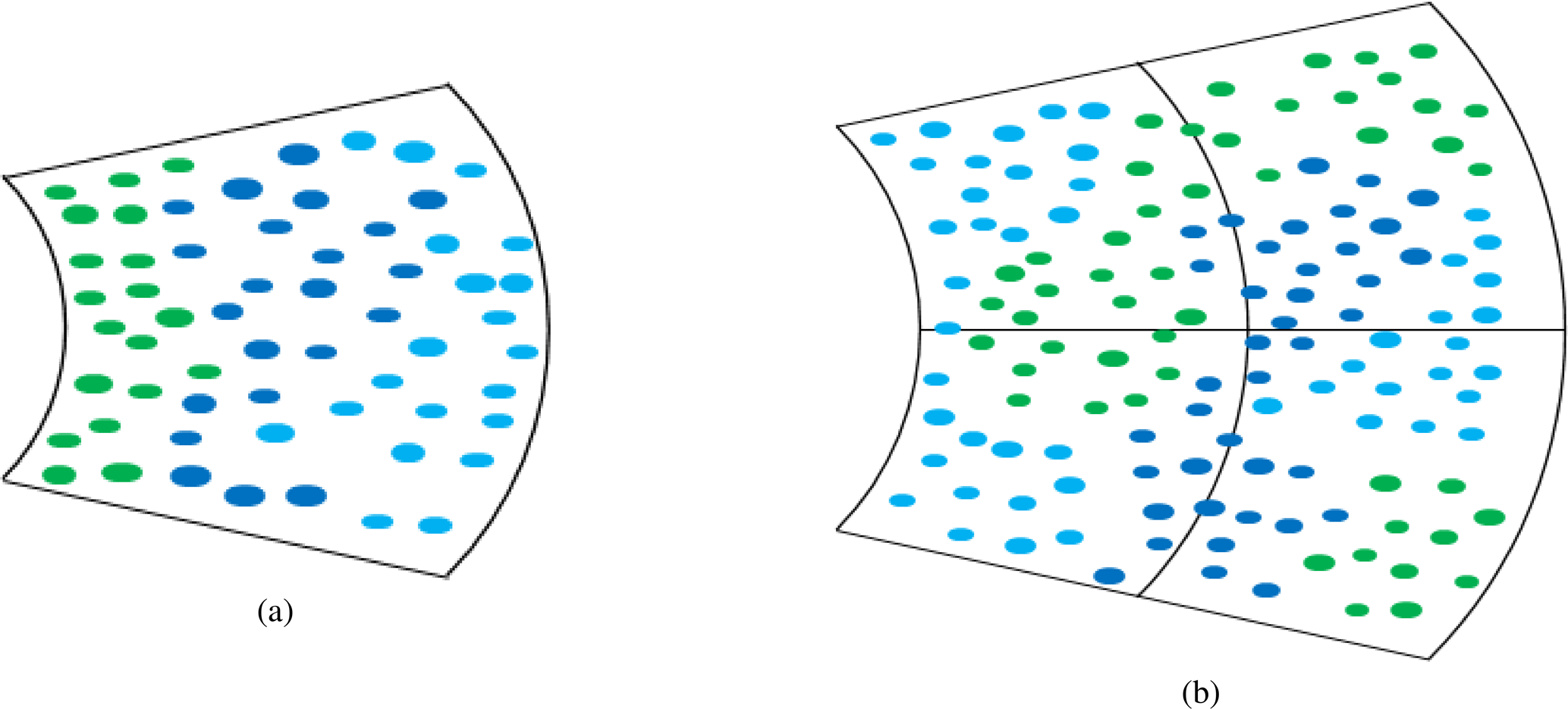
Figure 1 Simplified schematic representation of (a) bin-based de-mixing and (b) neighborhood-based analysis. In reality, the spatial organization of mixed hydrometeor types is presumed to be significantly more chaotic.

The article is organized as follows: in Sect. 2 we briefly introduce the polarimetric framework we rely upon in discriminating between different hydrometeor types as well as the more general concept of entropy in the context of radar remote sensing. In Sect. 3 we introduce and elaborate the bin-based approach, after describing the entropy parametrization. This section also contains the “Performance analyses” subsection, focused on the bin-based approach. In Sect. 4 we present the analysis, based on the conventional statistical techniques and dedicated to the incoherency in the mixed-radar sampling volumes. The subsequent evaluation subsection illustrates the impact of incoherency in the context of weather radar de-mixing. Section 5 concludes the article with a discussion and provides a series of perspectives for the presented work.

2 Polarimetric framework and the concept of entropy

The main objective of this paper could be summarized as drawing a parallel between the specific polarimetric framework of weather radar and the paradigm of decomposition/unmixing commonly used in SAR and hyperspectral remote sensing. The motivation for relying on the experience of SAR and hyperspectral communities comes from the demonstrated pertinence and utility of decomposition/unmixing in the data interpretation. This link we want to elaborate on, with the aim of de-mixing a weather radar sampling volume, is constructed around the common variable – entropy.

2.1 Polarimetric framework

The radar variables we rely upon to discriminate between different hydrometeor types are the reflectivity factor at horizontal polarization (Z_H), the differential reflectivity (Z_DR), the specific differential phase shift of propagation (K_dp) and the co-polar correlation (ρ_hv). The hydrometeor classification (Besic et al., 2016) and the bin-based de-mixing approach proposed in this article also consider a phase indicator (Ind), which can be derived from radar data in stratiform cases or from external information like ground observations or model simulations. This indicator takes the value $\text{Ind}\approx -\mathrm{1}$ for the liquid phase, Ind≈0 for the mixed phase and Ind≈1 for the solid phase (the approximative character is due to the employed sigmoid transformation of the relative altitude with respect to 0^∘ isotherm).

Due to the skewness and the leptokurticity (fatter distribution tails) of their distributions, K_dp and ρ_hv undergo the following logarithmic transformations: $K_{\mathrm{dp}}^{\prime }=\mathrm{10}\log (K_{\mathrm{dp}}+\mathrm{0.6})$ and ${\mathit{\rho }}_{\mathrm{hv}}^{\prime }=\mathrm{10}\log (\mathrm{1}-{\mathit{\rho }}_{\mathrm{hv}})$. Further on, all four radar variables are linearly scaled, i.e., min–max-transformed ([⋅]^scaled), to the $[-\mathrm{1},\mathrm{1}]$ range in the following limits: Z_H: −10 to 60 dBZ; Z_DR: −1.5 to 5 dB; $K_{\mathrm{dp}}^{\prime }$: −10 to 7; and ${\mathit{\rho }}_{\mathrm{hv}}^{\prime }$: −50 to −5.23.

Figure 2 The multi-dimensional (four out of five dimensions) space: (a) target vectors representing centroids (larger points with different classes depicted by different colors) and observations (smaller black points), (b) observations with assigned labels. Abbreviations: CRs – crystals; AGs – aggregates; LR – light rain; RN – rain; RPs – rimed ice particles; VI – vertically aligned ice; WS – wet snow; IH/HDG – ice hail/high-density graupel; MH – melting hail.

Therefore, each radar sampling volume is characterized by a five-element weather radar target vector,

$$\begin{array}{}\text{(1)}& \mathit{k}=\left[\begin{array}{c}{x}_{\mathrm{1}}\\ x_{\mathrm{2}}\\ x_{\mathrm{3}}\\ x_{\mathrm{4}}\\ x_{\mathrm{5}}\end{array}\right]=\left[\begin{array}{c}{Z}_{\mathrm{H}}^{\text{scaled}}\\ Z_{\mathrm{DR}}^{\text{scaled}}\\ K_{\mathrm{dp}}^{\text{'scaled}}\\ {\mathit{\rho }}_{\mathrm{hv}}^{\text{'scaled}}\\ \text{Ind}\end{array}\right],\end{array}$$

and can be represented as a point in a five-dimensional space formed by the five introduced parameters (Fig. 2a). The same space contains nine particular points, i.e., centroids (k_c), which represent the nine hydrometeor classes, and the classification itself comes down to the calculation of the Euclidean distance between the centroids and the observations (Fig. 2b):

$$\begin{array}{}\text{(2)}& d=\left|\right|{\mathit{k}}_{\mathrm{c}}-\mathit{k}|{|}_{\mathrm{2}},\end{array}$$

where $\left|\right|\cdot |{|}_{\mathrm{2}}$ is the ℓ₂ norm.

2.2 The concept of entropy

The concept of entropy (H) was introduced in radar polarimetry by Cloude and Pottier (1997) via the decomposition theory. It serves as an indicator of the usefulness of the polarimetry, demonstrating simultaneously important discriminating capabilities in the context of target classification. By equaling the proportion of n different components from the polarimetric decomposition to the probability of their occurrence (p_i), we obtain the entropy parameter, which converges towards 1 if we do not have a clearly dominant component (a “total” mixture) or towards 0 if we identify a clearly dominant component.

The min-entropy, being the minimum of Rényi's entropies (Rényi, 1960) and the originally proposed version of entropy estimator in Besic et al. (2016), is substituted here by the Shannon entropy estimator for the purpose of coherence with the conventional usage of the parameter in the remote-sensing community:

$$\begin{array}{}\text{(3)}& H=-\sum _{i=\mathrm{1}}^n{p}_i{\log }_n{p}_i,\end{array}$$

having values in the range [0,1].

The estimation of probabilities p_i, from now on occasionally referred to as proportions, is the focal point of the first part of this paper, i.e., the bin-based approach, proposed in the following section. A version of entropy, a bit closer to its original meaning in radar polarimetry (and therefore named H_CP – after Cloude and Pottier), with a slightly different nature of p_i, is used in the second part of the paper, studying the influence of potential spatial incoherency in backscattering in weather radar measurements.

3 Bin-based approach

The bin-based approach considers one volume at a time, without taking the neighboring spatial context into account. The proposed method is inspired by the SAR coherent polarimetric decomposition of elementary processes (e.g., Pauli and Krogager, Massonnet and Souyris, 2008) and the hyperspectral linear unmixing (Bioucas-Dias et al., 2012), and it is adapted to the context of the semi-supervised hydrometeor classification (Besic et al., 2016). Like its SAR role model, this method assumes the coherent summing of backscattering responses of different hydrometeors populating a radar sampling volume. This hypothesis is supported by the conventional averaging of backscattering information over a number of successive radar pulses, which aims to remove the influence of random spatial interferences.

Namely, the coherent decomposition of polarimetric SAR (PoLSAR) data relies on the first-order statistics and represents the scattering matrix of a target as a coherent sum of the scattering matrix of elementary interactions (odd bounce and double bounce with two different orientations). By comparing this to our polarimetric framework introduced in Sect. 2.1, we can deduce that our standard mechanisms, i.e., elementary interactions, would correspond to different hydrometeor classes. The important difference which prevents us from applying the equivalent formalism, even under the assumption of a total lack of interferences, is the orthogonality of the basis. That is to say, due to the different physical nature of the elements of the weather radar target vector (Eq. 1), which contains much less geometrical information than the scattering matrix, we cannot expect any orthogonality between the elementary hydrometeors or centroids. Therefore, the starting point of the bin-based de-mixing endeavor is to establish hydrometeor classes as elementary processes and to find a reliable, alternative way to sum them up, which somehow evades the lack of a real orthogonal basis.

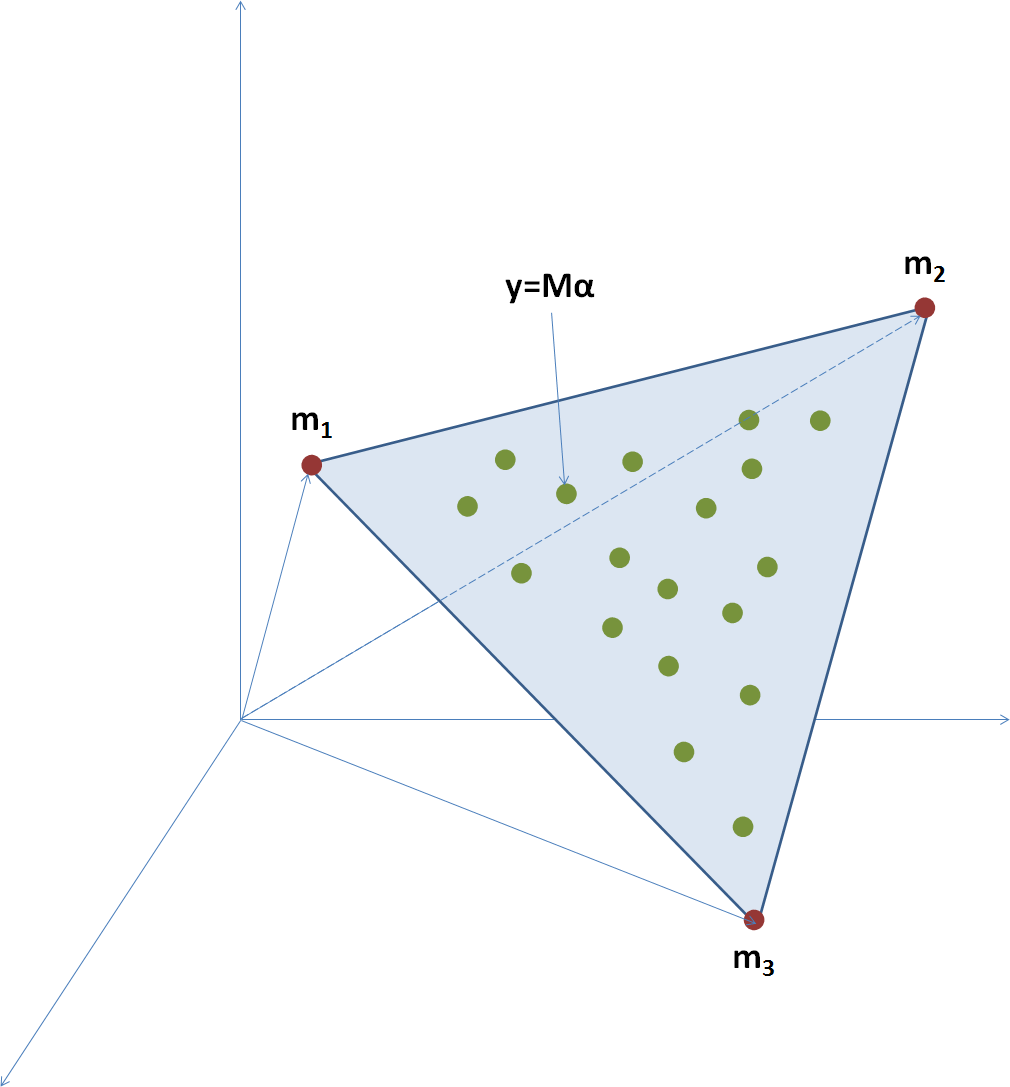
Figure 3 An example inspired by Bioucas-Dias et al. (2013) illustrating the problem of linear unmixing: blue simplex is defined by red m_i points depicting “pure” materials, whereas encompassed green points represent mixtures of these materials.

In terms of non-orthogonality, the hyperspectral linear unmixing problem appears more analogous to our polarimetric framework (Fig. 3). Namely, the target of the hyperspectral vector y contains the reflectance in n frequency bands and under the hypothesis of linearity can be represented as

$$\begin{array}{}\text{(4)}& \mathit{y}=\sum _{i=\mathrm{1}}^p{\mathit{\alpha }}_i{\mathit{m}}_i,\end{array}$$

where m_i is the vector of the ith “pure” material, i.e., end-member, while α_i would be its corresponding proportion. In the simplest of all cases, where we actually have the pure materials (e.g., types of ground or crop) among the observations, we are dealing with the so-called pure-pixel unmixing, where the method is reduced to the optimization problem:

$$\begin{array}{ll}{\displaystyle }& {\displaystyle }\underset{\mathbf{M},\mathbf{A}}{\text{min}}\left|\right|\mathbf{Y}-\mathbf{MA}|{|}_F\\ \text{(5)}& {\displaystyle }& {\displaystyle }\text{subject to }\mathbf{A}\ge \mathbf{0},{\mathit{I}}_p^T\mathbf{A}={\mathit{I}}_n,\end{array}$$

with Y being the matrix of observations, $\left|\right|\mathbf{X}|{|}_F=\sqrt{\mathrm{trace}\left({\mathbf{XX}}^T\right)}$; A the matrix containing the proportions of every end-member in every observation; and M the matrix containing end-members. Column vectors I_p and I_n are respectively p- and n-long vectors of ones. The problem can be represented geometrically as the estimation of a simplex around the observations, as illustrated in Fig. 3.

When comparing Figs. 2a and 3, one can notice the intuitive similarity of the problem: estimating proportions of pure components by considering their distances from the observations. However, the major obstacle in applying the very efficient paradigm of the spectral unmixing to the particular context of hydrometeor de-mixing is the fact that our centroids do not really represent the end-members in the five-dimensional space. Namely, the target vectors corresponding to centroids are supposed to be the representative examples of different classes, and they are thus not represented by the extreme values of our polarimetric parameters. Nevertheless, basing the estimates of proportions on the distance in the space populated by the standard mechanisms (centroids) and measurements is a reasonable way to sum up the standard mechanisms.

Now that we have identified our centroids as standard mechanisms (analogy with PolSAR) and have found a mode for their addition via the distances in the Euclidean space of the classification, we have to adapt the latter to the particular nature of the former. That is to say, our centroids do not form a regular structure (e.g., cube), where under the assumption of coherence and linearity the distance of a measurement with respect to the standard mechanism could be directly interpreted as the probability, i.e., as the proportion of the given standard mechanism. They are rather non-uniformly distributed in the five-dimensional space. In order to deal with this, we adopted the varying slope exponential transformation of the distance between the measurement and the ith centroid (d_i) to the probability (p_i), i.e., the proportion of the hydrometeor class i depicted by the centroid in the measurement. The exponential function is chosen in order to account for the uncertainty around the centroid (p has higher values in the vicinity of the centroid), while the varying slope (t_i) accounts for the irregular distribution of the centroids in the classification space:

$$\begin{array}{}\text{(6)}& p_i=e^{-t_i{d}_i},i=\mathrm{1},\mathrm{\dots }\mathrm{8}\left(\mathrm{9}\right).\end{array}$$

Namely, t_i depends on the assigned classification label, which is basically the nearest centroid to the measurement (c_i). The idea here is for a probability to drop to a threshold value p_t at the distance corresponding to the separation between c_i and c_closest – the closest centroid to the one determining the label (Fig. 4):

$$\begin{array}{}\text{(7)}& p_{\mathrm{t}}\approx e^{-t_{i}d({\mathit{c}}_i,{\mathit{c}}_{\mathrm{closest}})},\end{array}$$

which results in

$$\begin{array}{}\text{(8)}& t_i={\displaystyle \frac{\ln \frac{\mathrm{1}}{p_{\mathrm{t}}}}{d({\mathit{c}}_i,{\mathit{c}}_{\mathrm{closest}})}}.\end{array}$$

Figure 4 An example of the exponential transformation: the scaled distances to the probability (d→p).

The threshold value of probability (p_t) is determined using a synthetic dataset, created by linearly mixing different pairs of hydrometeor classes in equal proportions (an example is given in Fig. 5). Each pure hydrometeor box contains 900 synthetic realizations of hydrometeors varying uniformly in the very restricted interval around the values of the corresponding centroid (−1 % to 1 %, in order to emphasize the hypothesis of the “pureness”). Boxes of hydrometeor mixtures contain different versions of mostly plausible mixtures obtained by linearly combining in equal shares polarimetric parameters of two hydrometeor types involved, following assumptions of coherence and linearity. Linear combination here stands for the arithmetic mean (equal proportions) in each dimension of the five-dimensional classification space. Each of these boxes again contains 900 synthetic realizations, where each realization represents a presumingly equiprobable mixture. We opted for this “quadratic” organization of boxes, in order to indicate the limitations of the proposed approach as well, aside from obviously emphasizing the plausible mixtures.

It would be indeed even more precise to combine the mixing components at the level of the electromagnetic scattering, before the integration leading to the employed polarimetric parameters. However, not event this would help us overcome the unavoidable lack of methodological “transparency” in terms of physics, due to the absence of the orthogonal de-mixing basis. The proposed method is therefore rather defined in a more empirical fashion, in the data processing plane, with the physical trustworthiness being verified experimentally, mostly using the independent measurements.

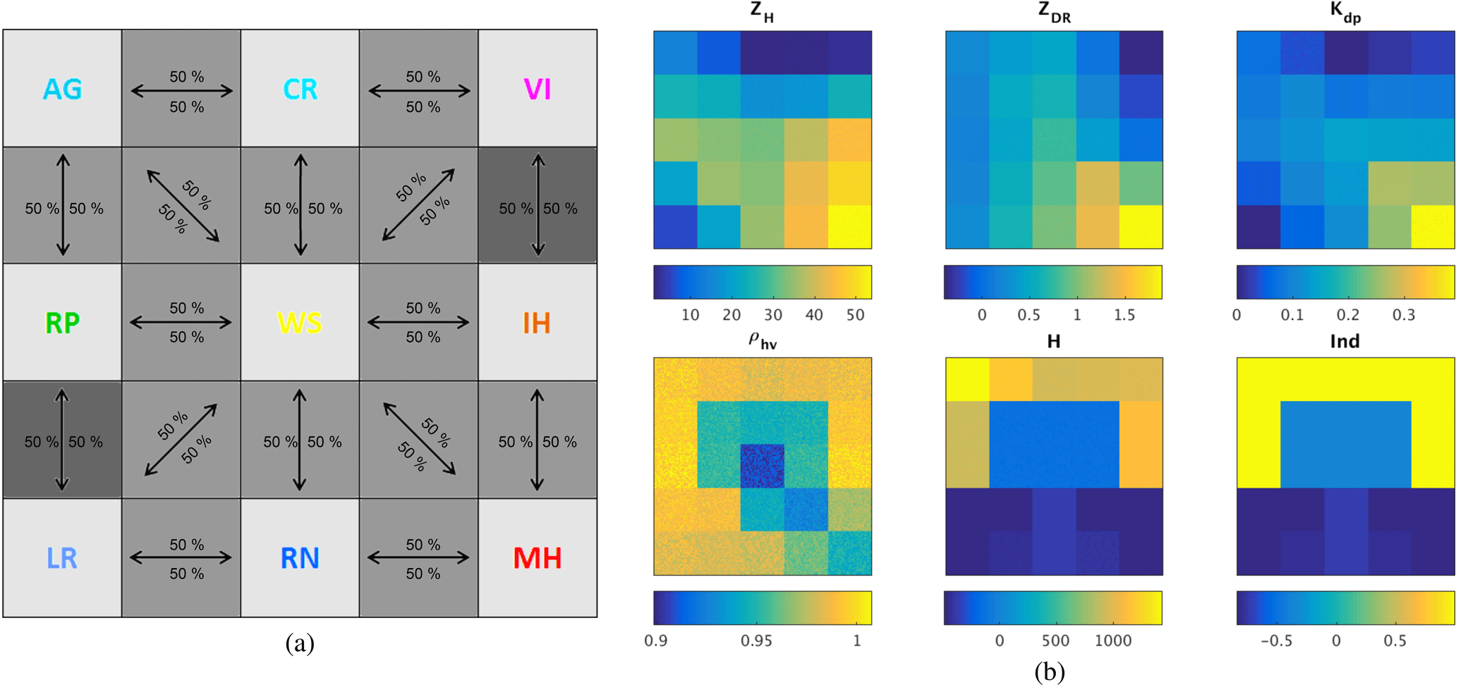
Figure 5 Quadratically organized synthetic dataset used in the entropy parametrization: (a) the plan with pure hydrometeors (light gray), mixtures (gray), and not very plausible mixtures (dark gray); (b) the value of elements of weather radar target vector (including the relative altitude with respect to the 0^∘ isotherm – H).

Applying the hydrometeor classification to the synthetic dataset results in an expectedly proper recognition of pure hydrometeor boxes (Fig. 6). The mixed hydrometeor boxes are identified as an ensemble of both hydrometeor classes involved in the mixing, as an ensemble of only one of the classes involved in the mixing or as an ensemble of the classes which are not presumed to be involved in the mixing. The latter case, which mostly relates to the less plausible mixtures, represents the sort of limitation of the method (primarily boxes marked with the darkest shade of gray in Fig. 5a), but the co-existence of two classes with very distinct polarimetric properties (particularly in terms of Z_H) is indeed physically not very probable. However, in these critical cases, the presence of the identified class which was not involved in the mixing process can still be justified, e.g., when the mixture of melting snow and melting hail contains some rain or the mixture of ice hail and vertical ice contains aggregates and rimed particles.

The parameterized entropy, obtained by substituting p_i in Eq. (3) with the one from Eq. (6), indeed shows very low values in the case of pure hydrometeors (Fig. 6). The synthetic hydrometeor mixtures are, on the other hand, characterized by higher entropy values. This is true even for the less plausible mixtures mentioned in the previous paragraph, where the bin-based mixing approach reaches its limitations.

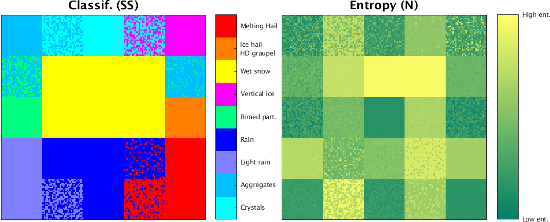
Figure 6 Classification and entropy applied to the synthetic dataset from Fig. 5. Low and high entropy values correspond to the limits of the range [0,1].

The utility of the proposed parameterization of entropy, which is based on the estimated proportions of different hydrometeors involved in a mixture, can be adequately illustrated using the exemplary data introduced in Fig. 2. In Fig. 7 we show the comparison between the original and the parameterized version of entropy values for the considered data samples. The increased values of entropy between the “mixable” neighbor centroids reflect clearly the results obtained with synthetic datasets. The limitation of the method can also be more clearly conceived here, because the mixtures of extreme points (e.g., vertical ice and ice hail) unavoidably finish close to the centroids in between.

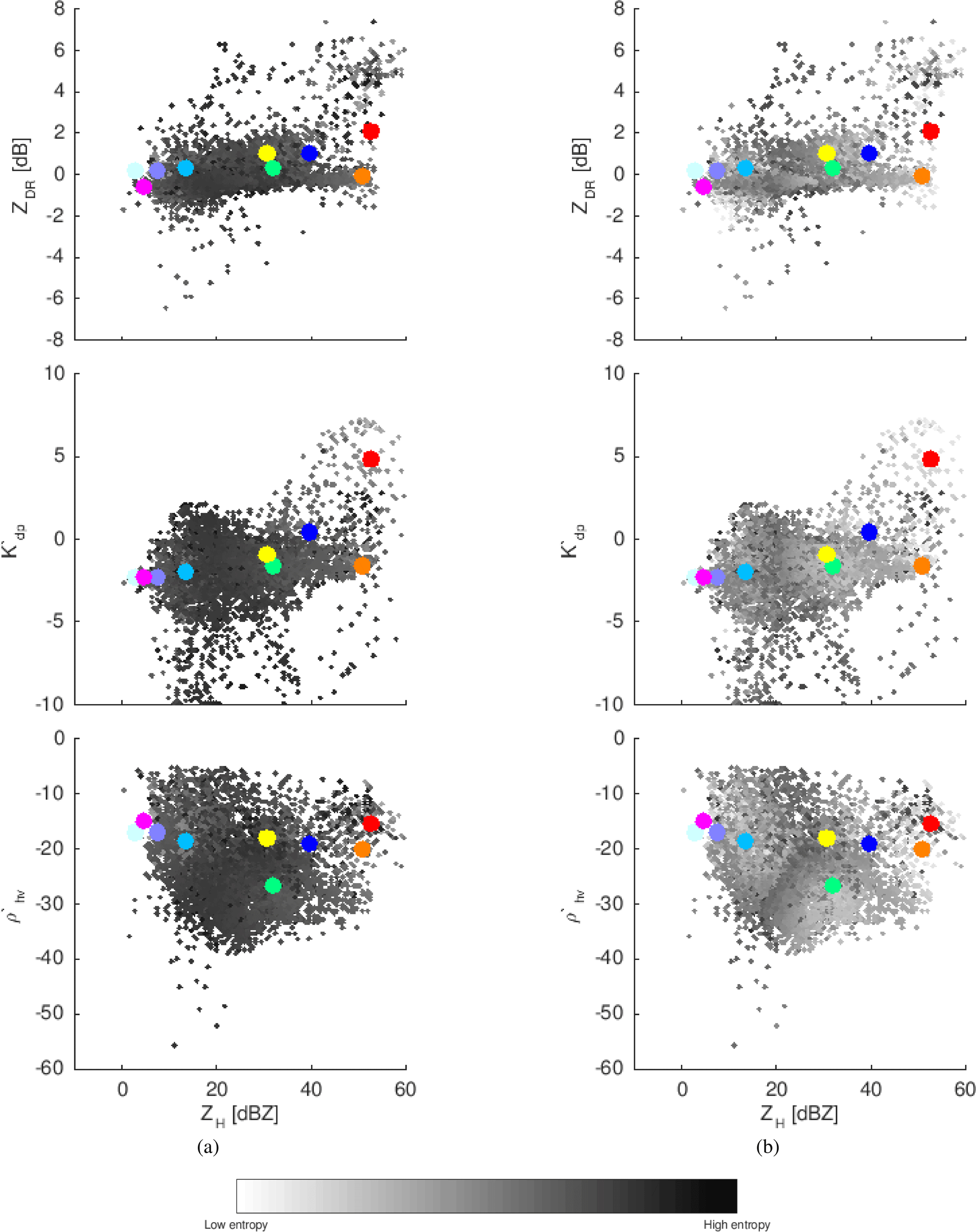
Figure 7 The multi-dimensional (four out of five dimensions) space, with target vectors representing centroids (larger points with different classes depicted by different colors) and observations with the level of gray depicting (a) Shannon version of the entropy from Besic et al. (2016) and (b) parametrized entropy.

Before proceeding to the performance analysis, in order to quantify the potential implicit biases of the introduced parameterization, we apply the de-mixing method to the particular combinations of hydrometeors mixed in both equal and non-equal proportions. Namely, as illustrated in Fig. 8 we consider the mixtures of AG–CR, AG–RP and RN–MH (see figure caption for abbreviation definitions) in the following proportions: 75 %–25 %, 60 %–40 %, 50 %–50 %, 40 %–60 % and 25 %–75 %.

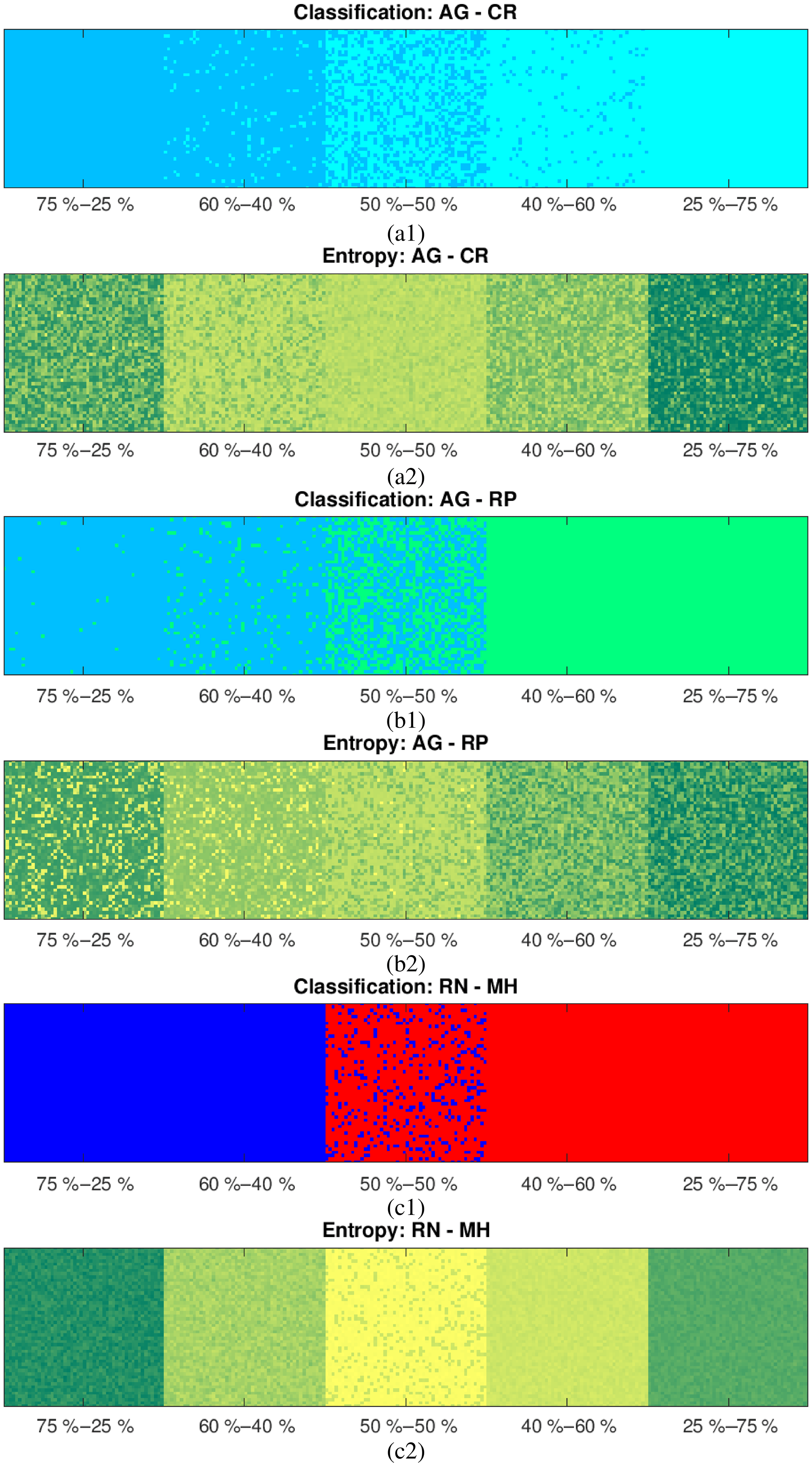
Figure 8 Classification (1) and entropy (2) for different combinations of synthetically produced mixtures: (a) aggregates–crystals, (b) aggregates–rimed ice particles and (c) rain–melting hail.

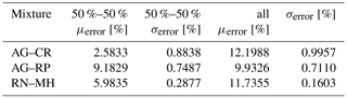
Quantification of the results presented in Fig. 8, provided in Table 1, shows that a mean error for the 50 %–50 % combination does not exceed 9.2 % with a very small standard deviation (<1 %), meaning that we definitely do much better than the classification without de-mixing, which in this case can cause a 50 % error. A mean error for all combinations does not exceed 12.2 % with a very small standard deviation (<1 %), showing again that we necessarily do far better than the classification without the de-mixing.

Table 1 Quantitative evaluation of de-mixing errors (biases) obtained using synthetic (simulated) dataset.

3.1 Performance analyses

The performance of the introduced bin-based method is analyzed hereby in three respective stages, very characteristic for the validation of techniques related to the hydrometeor classification: spatial plausibility, comparison between two radars and comparison between a radar and a ground level instrument.

3.1.1 Spatial plausibility

In Fig. 9a1 we show an example of the classification applied to the MXPol X-band radar data acquired at the Dumont-d'Urville base, on the coast of Antarctica, during the Antarctic Precipitation, Remote Sensing from Surface and Space (APRES3) campaign (Grazioli et al., 2017). Given the systematically low temperatures at the ground level, in the illustrated range height indicator (RHI), only solid-phase hydrometeors are identified. By analyzing the estimation of entropy, we can notice a rise in the entropy characterizing bordering regions between aggregation and riming. The high probability of mixing and misclassification of aggregates and rimed particles is due to the similarity in their polarimetric signatures and their spatial co-occurrence. Furthermore, in the context of meteorology, aggregates and rimed particles are not so distinct classes (a frequent phenomenon, riming of aggregates, is identified as rimed ice particles (RPs) by the employed classification). All this calls for particular attention to this challenging and relevant de-mixing problem in the performance analyses. This is also sustained by the special interest in the riming identification due to its role in better understanding the orographic precipitation mechanisms (Grazioli et al., 2015a; Houze and Medina, 2005).

The results of the bin-based de-mixing, illustrated in Fig. 9b, do not indicate the presence of hydrometeors other than the ones identified as dominant in Fig. 9a. However, they indicate the significant percentage of aggregates in the volumes labeled as rimed ice particles and vice versa, as could be intuitively expected from the entropy estimate. The first stage of the performance analyses would be exactly the spatial continuity of this observation, i.e., the fact that the percentage of rimed particles decreases progressively as we move away from the region labeled as rimed particles, the same being true for aggregates. No matter how simple this may seem, given that we are dealing with a bin-based method, which does not consider at all the spatial context, the observed spatial continuity can indeed be considered as the very first positive indicator of reliable performances.

Figure 10a depicts an example of the classification of a hail cell and its surrounding, observed by the MXPol X-band radar during the HYdrological cycle in the Mediterranean EXperiment (HyMeX) campaign (Bousquet et al., 2015; Ducrocq et al., 2014). The results of the bin-based de-mixing (Fig. 10b) again show the smooth and plausible transition between the lower part of the hail cell and the surrounding rain, with the borders of the cell (as defined by the classification) representing the intense mixing. The same situation is noted in the upper part of the cell, where hail mixes with the encircling rimed ice particles.

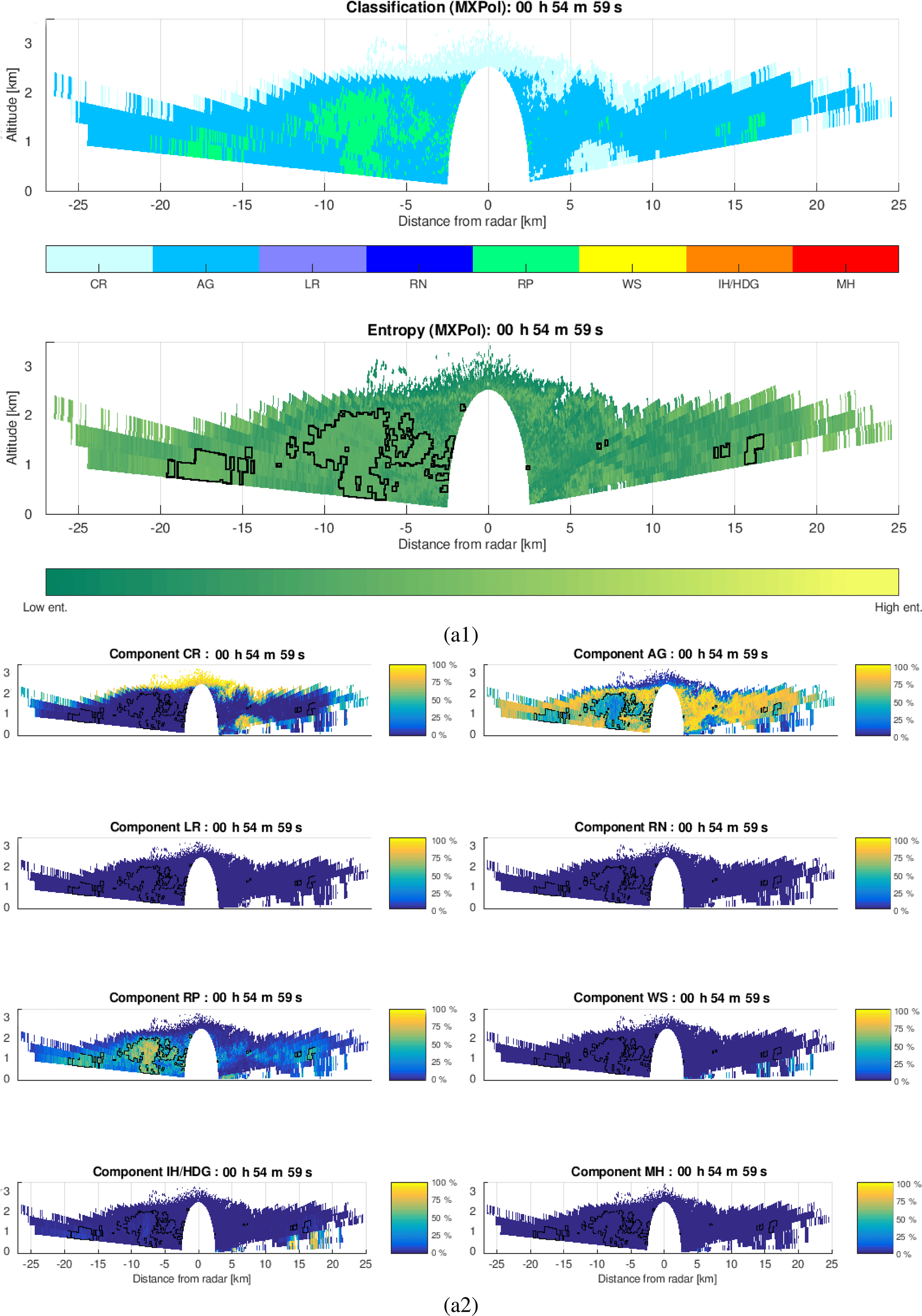
Figure 9 Bin-based de-mixing applied to an example MXPol dataset acquired during the APRES3 campaign at the Dumont-d'Urville base, Antarctica, on 28 January 2016: (a) classification followed by the entropy estimate, (b) proportion of eight hydrometeor classes in each of the radar sampling volumes.

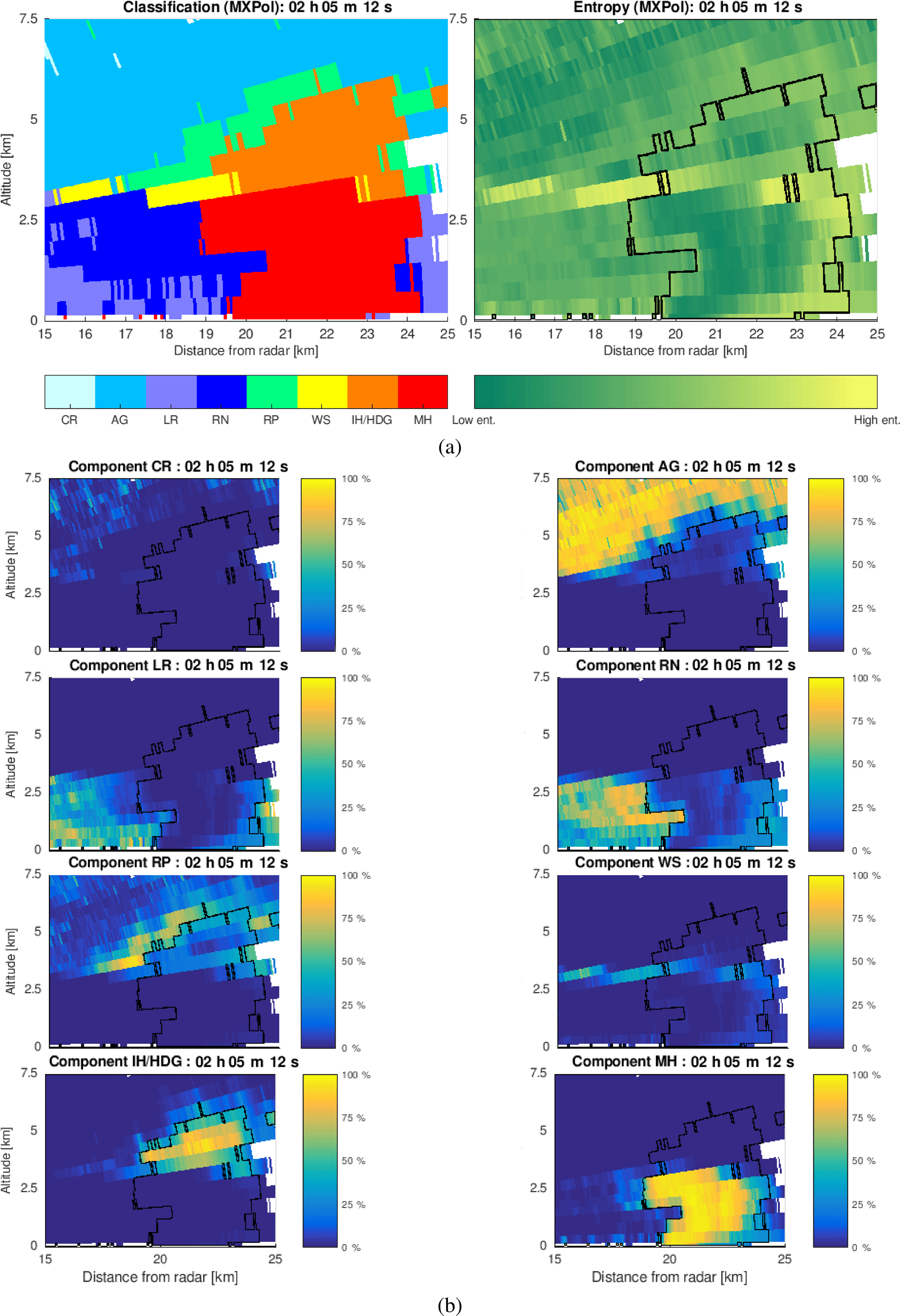
Figure 10 Bin-based de-mixing applied to an example MXPol dataset acquired during the HyMeX campaign in the region of Ardèche, France, on 24 September 2012: (a) classification followed by the entropy estimate, (b) proportion of eight hydrometeor classes in each of the radar sampling volumes.

3.1.2 Inter-radar comparison

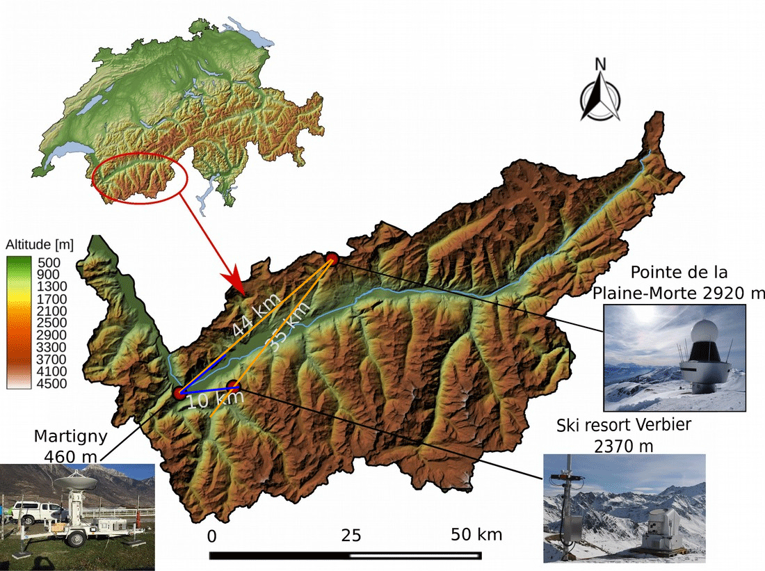
The following two stages of the performance verification are related to the measurement campaign organized in the Swiss canton of Valais, from November 2016 to April 2017. The campaign was based on the careful collocation of different instruments, depicted in Fig. 11: MeteoSwiss operational C-band radar at Pointe de la Plaine Morte (2920 m a.s.l.), MXPol X-band radar (460 m a.s.l.) and the MASC (2370 m a.s.l.; Garrett et al., 2012).

Not having the possibility to retroactively manipulate the scanning strategy, we decided to base the second step of the verification on analyzing the influence of the proposed de-mixing method on the classification matching between two radars covering a certain common volume. Namely, we defined the vertical cross section sized 7 km in range and 2 km in height, being common for the Plaine Morte radar 227^∘ and the MXPol radar 47^∘ azimuthal RHI (see blue and orange segments in Fig. 11). Further on, we selected a period of 50 min, corresponding to 10 acquisitions by the Plaine Morte radar (plan position indicators (PPIs) and therefore reconstructed RHIs) and 14 RHI acquisitions by the MXPol radar (5:05–5:55 UTC on 28 February 2017), where the stationarity in terms of proportions of dominant labeled hydrometeors could be assumed.

Figure 11 Configuration of instruments deployed during the Valais campaign.

One of the acquisitions, illustrated in Fig. 12a, shows a clear difference in the sampling volume size between two radars. Namely, although the range resolutions of the two radars are indeed comparable (75 m for the MXPol radar and 83 m for the Plaine Morte radar), the vertical cross section is significantly closer to the MXPol radar, which makes it have much better azimuthal resolution as well. Entropy estimations in Fig. 12b show an overall significant rise in the entropy values for the Plaine Morte radar, with respect to the ones of the MXPol radar. Due to the expected increase in hydrometeor mixing with the increase of the radar sampling volume, this observation, supported by other analyzed acquisitions, confirms the crucial role of the parameterized entropy in detecting hydrometeor mixtures. It therefore confirms the plausibility of the proposed bin-based approach, intrinsically related to the concept and the definition of the entropy parameter.

With the data being kept in polar coordinates, it was impossible to properly match the volumes. Thus, a more direct, quantitative way of proving the utility of the proposed de-mixing approach comes down to the comparison of the proportions of detected classes in the entire cross section, before and after the de-mixing (Fig. 12c–e). The quantitative mismatching criterion is the simple measure of distance between the normalized proportions of hydrometeors seen by the MXPol radar (PR_MX) and by the Plaine Morte (PR_PM):

$$\begin{array}{}\text{(9)}& D={\displaystyle \frac{{\sum }_{i=\mathrm{1}}^{\mathrm{4}}{\mathrm{PR}}_{\mathrm{MX}}^i-{\mathrm{PR}}_{\mathrm{PM}}^i}{{\sum }_{i=\mathrm{1}}^{\mathrm{4}}|{\mathrm{PR}}_{\mathrm{MX}}^i{|}^{\mathrm{0}}\bigvee |{\mathrm{PR}}_{\mathrm{PM}}^i{|}^{\mathrm{0}}}},\end{array}$$

normalized by the number of classes detected either by one or by both instruments (logical or operator, in the denominator). The value of D, averaged over all considered scans, is provided in the titles of Fig. 12c–e.

In Fig. 12d the de-mixing is limited to the proportions of the first three dominant components, which tend to occupy the majority of the radar sampling volume, and are not likely to account for only the residual presence of a hydrometeor class. This comparison shows not only the improved matching but also the presence of hydrometeors unidentified before the de-mixing. Extending the de-mixing to all eight components (VI being merged with CR) furthermore improves the matching, at the expense of the occurrence of residually present classes (WS in this case).

The share of the dominant class (Fig. 12f and g) would be the quantitative confirmation of the logical assertion made in the previous paragraph: in the case of a bigger radar sampling volume, with the proposed method we tend to infer more mixing.

We also benefited from this configuration checking for the potential correlation between the entropy parameter/mixture indicator H and polarimetric parameters constituting the weather radar target vector (Eq. 1). The weak but statistically significant linear correlation (at .05 significance level) of −0.4 for MXPol and −0.17 for the Plaine Morte radar is observed for the co-polar correlation (ρ_hv), which makes quite a bit of sense given that ρ_hv is often interpreted as a measure of heterogeneity.

Figure 12 Comparison example in terms of classification (a) and entropy (b) between Plaine Morte (1) and MXPol (2), followed by the quantitative matching analysis before de-mixing (c), after de-mixing with only three dominant components (d) and after de-mixing with all components(e), and quantitative measure of mixing ratio with only three components (f) and with all components (g).

3.1.3 Comparison with the ground level observations

The final stage of the verification is based on comparing the outcome of the de-mixing method with the classification of individual particles from the ground level instrument. The principle intuitively resembles the comparison with classification based on the 2-Dimensional Video Disdrometer (2DVD) (Grazioli et al., 2014) in the original classification paper (Besic et al., 2016). The classification of MASC images is described in Praz et al. (2017). Using a supervised machine learning approach, it distinguishes between small particles (SPs), columnar crystals (CCs), planar crystals (PCs), a combination of columnar and plate crystals (CPCs), aggregates (AGs) and graupel (GR), with the additional possibility of estimating a degree of riming and determining whether the particle is melting or not. In order to make the comparison possible, we formed the corresponding merged classes: CR ($\mathrm{CC}+\mathrm{PC}+\mathrm{CPC}$), AG (AG), RP (GR) and MS (any of the classes with the melting degree different from zero). Evidently, neither the MASC as the instrument nor the classification applied to its measurements can be considered as an ideal reference. The major limitations which ought to be considered when analyzing the results presented in this section are the possible occurrence of blowing snow, the limited sampling volume of the instrument, the quality of recorded images and the inevitable classification random errors.

The setup is again based on considering the vertical cross section of the reconstructed RHI of the Plaine Morte radar, though this time in a slightly more restricted area of 4 km in the range direction, around the MASC (Fig. 13a and b). The unavoidable difference in height between the MASC and the lowest (non-clutter-contaminated) considered radar sampling volume could hypothetically compromise the comparison given the microphysical processes which can occur in this non-observed region. However, given the relative nature of the comparison (before and after de-mixing), as well as the employed spatial and temporal averaging, this effect is fairly limited.

In order to fully satisfy the hypothesis of stationarity (in terms of proportions of dominant labeled hydrometeors), which allows us to properly average the de-mixing scores, we selected different periods across different events, summarized in Table 2. The quantitative matching criterion is identical to the D defined in Eq. (9), with Pr_MX being replaced by Pr_MASC.

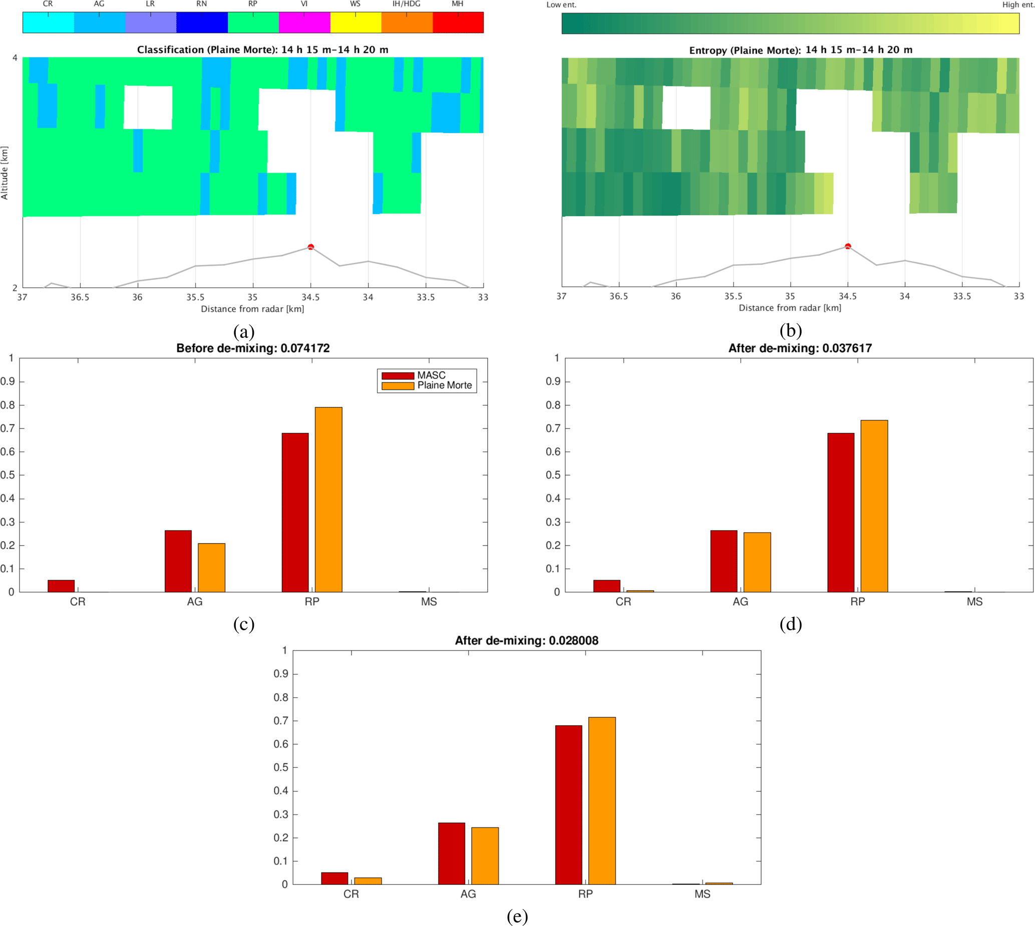
Figure 13 Comparison of classification applied to Plaine Morte data (a, b) with the MASC classification, before de-mixing (c) and after de-mixing: with the three dominant components (d) and with all components (e).

Table 2 Quantitative scores (D) of the Plaine Morte–MASC comparison before and after the bin-based de-mixing. Events 3 and 5 are illustrated respectively in Figs. 13 and 14.

Though the quantitative evaluation of mismatching shows pretty good results from the classification itself, similarly to the second stage of the verification, we can still notice that in all six analyzed events, regardless of their duration, the applied de-mixing method improves the distribution matching (smaller D). The matching also systematically appears to be better if we consider all components, rather than the three dominant ones. The improvement in matching is also correlated with the measure of entropy averaged over the event and the vertical cross section (μ(H)). Namely, lower μ(H) means smaller probability of mixing and therefore more limited potential in terms of distribution matching.

In Fig. 13c–e we illustrate how the distributions actually compare across four merged classes. The presented event (no. 3 in Table 2) highlights the improved agreement in terms of concentration of AGs and RPs. It also shows the risk of overestimating residually present particles (MS in this case) in the case of the extension to all eight de-mixing components (Fig. 13e).

In order to demonstrate the capability of the method of dealing with the hydrometeor classes other than the over-represented aggregated and rimed ice particles, we illustrate the comparison of distributions across four classes for event no. 5 in Fig. 14. Namely, it was the warmest day with a significant amount of precipitation during the campaign, and our hope was to perform some de-mixing around the melting layer. Unfortunately, though the MASC was effectively in the melting layer, the lowest radar beam was 400–500 m above the 0^∘ isotherm, and MXPol data happen to be compromised by ground clutter in the direction of interest. Nevertheless, the de-mixing shows very good performances in estimating the proper percentage of the third class involved – crystals (Fig. 14b and c).

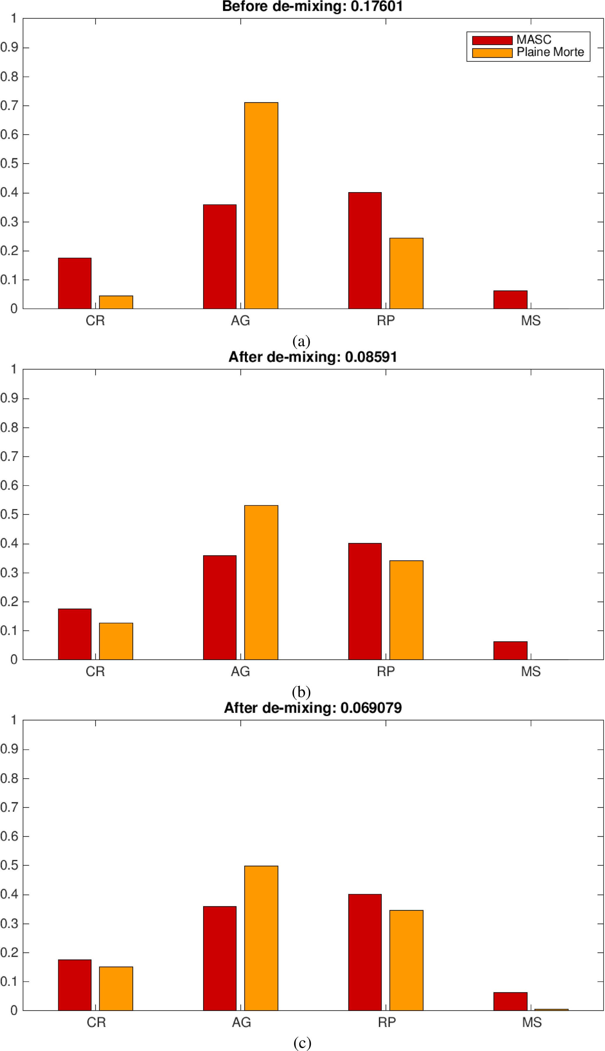
Figure 14 Comparison of classification applied to Plaine Morte data with the MASC classification, before de-mixing (a) and after de-mixing: with only three de-mixing components (b) and with all de-mixing components (c).

The agreement with the MASC is further reinforced by considering the additional parameter estimated from the MASC measurements – the continuous riming degree index (DoR) (Praz et al., 2017). Independent from the previously mentioned classification, DoR is defined in the range between 0 (no riming) and 1 (graupel). Relying on the previously introduced setup, we now only consider the proportion of rimed ice particles detected by the radar (before and after de-mixing) and the proportion of particles characterized as rimed with a different level of strictness with respect to the DoR (DoR≥N, with N being a riming threshold).

Figure 15 Radar vs. MASC, detection of rimed particles: (a) temporal evolution of event no. 2, with the shades of gray corresponding to different thresholds (≥) applied to DoR (dark corresponding to 0.5; light corresponding to 1), green dashed line being the proportion of RPs before the de-mixing and green solid line being the proportion of RPs after the de-mixing; (b) cross correlation for all events from Table 2; and (c) root mean square error (RMSE) for all events from Table 2.

In Fig. 15a we can see an example (event no. 2) of the temporal evolution of the proportion of the RPs as seen by the radar before and after the de-mixing, versus the proportion of rimed particles as seen by the MASC for different thresholds applied to DoR. The moderate temporal correlation which can be intuited from this example is quantified in Fig. 15b for the merged observations from all six events. By introducing the temporal dimension into the analysis, we can deduce that the correlation actually slightly decreases after the de-mixing, though not significantly. By checking for the time-lagged correlation, we see that the vertical trajectory between the lowest radar sampling volume and the MASC does not seem to compromise significantly the time matching of the samples. Finally, still considering the merged observations, by looking at the root mean square error between the estimated proportions for different DoR thresholds in Fig. 15c, one can notice a significant improvement introduced by the de-mixing method.

4 Neighborhood-based analysis

The neighborhood-based analysis is founded on simultaneously considering an ensemble of pixels, rather than one pixel at a time as was the case with the bin-based approach. This approach increases the potential issue of the spatial incoherency in weather radar measurements (Tso and Mather, 2009), a phenomenon which is conveniently neglected in the previously presented bin-based approach, even though it could potentially be considered relevant in the context of hydrometeor mixtures. Namely, given that the size of the hydrometeors populating the sampling volume is inferior to the size of the volume itself, the conventional radar measurements are affected by the random spatial interference of the scattered waves (otherwise known as the speckle effect), causing the incoherency in the measurements. It is important to state that the precipitation has also been characterized as a partly coherent scatterer (Jameson and Kostinski, 2010a, b), even though the former is more commonly associated with the clutter response (Zhang, 2016). Averaging the parameters over several pulse responses, i.e., obtaining the estimates from time averages of auto- and cross-correlations of received echoes (Balakrishnan and Zrnic, 1990; Sauvageot, 1982), conventionally serves as a sort of speckle filter, which should deal with the incoherency by canceling the random interferences. This technique is presumed to be efficient in the case of measurements corresponding to incoherent scattering, whereas in the case of non-random interferences (coherent scatterer) its usefulness remains questionable.

In the radar sampling volume populated by different hydrometeor types (characterized by significantly different shapes and fall velocities), it is logical to suspect that some residual interferences could “survive” the conventional averaging over several pulses. Embracing the hypothesis of originally incoherent measurements, one could consider this to be the residual incoherency, though this could equally be an intrinsically coherent backscattering as described by Jameson and Kostinski (2010a, b). However, in the context of de-mixing, only the residual incoherency really potentially compromises the proposed bin-based approach, which is fundamentally based on first-order statistics – the vectors representing centroids. That is to say, the presence of incoherency in backscattering would require relying on at least second-order statistics in evaluating a mixture.

This being said, we decided to proceed with the following analysis, inspired by SAR incoherent polarimetric decompositions (Cloude and Pottier, 1996) and adapted to our specific polarimetric framework introduced in Sect. 2.1. The actual idea behind it is that, by considering the spatial ensemble of integrated radar responses over radar sampling volumes, we can assess the level of the “surviving” random interference of individual hydrometeor responses inside a radar sampling volume. Therefore, the following analysis can be considered as a way of diagnosing, by means of assessing the spatial consistency, the presence of the hereby described residual spatial incoherency. It is important to keep in mind that this technique most probably cannot distinguish the very small scale coherency in backscattering from the residual incoherency.

It should be noted that the phase indicator, as external information, is not included (phase indicator, the fifth element of our weather radar target vector (Eq. 1), meaning that from now on k is a four-element vector).

4.1 PCA

Principal component analysis is a statistical method which transforms the data represented in a space formed by correlated variables to the space formed by orthogonal, linearly uncorrelated variables (Pearson, 1901). By assuming that our data samples represent points in the space formed by four transformed and linearly scaled polarimetric variables (${\left[x_{\mathrm{1}}{x}_{\mathrm{2}}{x}_{\mathrm{3}}{x}_{\mathrm{4}}\right]}^T$), the PCA comes down to the eigenvector decomposition of the sample estimated (〈⋅〉) covariance matrix of data samples. This allows us to describe the covariance matrix as a weighted sum of covariance matrices of the eigenvectors, i.e., the principal components k_i:

$$\begin{array}{ll}{\displaystyle }〈\mathit{k}{\mathit{k}}^T〉& {\displaystyle }=〈{\left[x_{\mathrm{1}}{x}_{\mathrm{2}}{x}_{\mathrm{3}}{x}_{\mathrm{4}}\right]}^T\left[x_{\mathrm{1}}{x}_{\mathrm{2}}{x}_{\mathrm{3}}{x}_{\mathrm{4}}\right]〉=\\ \text{(10)}& {\displaystyle }& {\displaystyle }={\mathit{\lambda }}_{\mathrm{1}}{\mathit{k}}_{\mathrm{1}}{\mathit{k}}_{\mathrm{1}}^T+{\mathit{\lambda }}_{\mathrm{2}}{\mathit{k}}_{\mathrm{2}}{\mathit{k}}_{\mathrm{2}}^T+{\mathit{\lambda }}_{\mathrm{3}}{\mathit{k}}_{\mathrm{3}}{\mathit{k}}_{\mathrm{3}}^T+{\mathit{\lambda }}_{\mathrm{4}}{\mathit{k}}_{\mathrm{4}}{\mathit{k}}_{\mathrm{4}}^T,\end{array}$$

with the weights λ_i being the corresponding eigenvalues. The obtained eigenvectors should represent scatterers, in our case types of hydrometeors, incoherently mixed in the considered data (X). By projecting the original incoherent dataset values X onto the set of eigenvectors, we obtain the dataset values in the new space – Y. These new values could be taken for the measurements as they presumingly should be if it were not for the incoherence in the measurements:

$$\begin{array}{ll}{\displaystyle }\mathbf{Y}& {\displaystyle }=\left[\begin{array}{cccc}{y}_{\mathrm{11}}& y_{\mathrm{12}}& y_{\mathrm{13}}& \mathrm{\cdots }\\ y_{\mathrm{21}}& y_{\mathrm{22}}& y_{\mathrm{23}}& \mathrm{\cdots }\\ y_{\mathrm{31}}& y_{\mathrm{32}}& y_{\mathrm{33}}& \mathrm{\cdots }\\ y_{\mathrm{41}}& y_{\mathrm{42}}& y_{\mathrm{43}}& \mathrm{\cdots }\end{array}\right]={\left[{\mathit{k}}_{\mathrm{1}}{\mathit{k}}_{\mathrm{2}}{\mathit{k}}_{\mathrm{3}}{\mathit{k}}_{\mathrm{4}}\right]}^T\mathbf{X}=\\ \text{(11)}& {\displaystyle }& {\displaystyle }={\left[{\mathit{k}}_{\mathrm{1}}{\mathit{k}}_{\mathrm{2}}{\mathit{k}}_{\mathrm{3}}{\mathit{k}}_{\mathrm{4}}\right]}^T\left[\begin{array}{cccc}{x}_{\mathrm{11}}& x_{\mathrm{12}}& x_{\mathrm{13}}& \mathrm{\cdots }\\ x_{\mathrm{21}}& x_{\mathrm{22}}& x_{\mathrm{23}}& \mathrm{\cdots }\\ x_{\mathrm{31}}& x_{\mathrm{32}}& x_{\mathrm{33}}& \mathrm{\cdots }\\ x_{\mathrm{41}}& x_{\mathrm{42}}& x_{\mathrm{43}}& \mathrm{\cdots }\end{array}\right].\end{array}$$

Going backwards, by applying the inverse PCA transform, we can estimate the proportions of the originally measured samples contributing to each of the pure uncorrelated components:

$$\begin{array}{}\text{(12)}& {\mathbf{X}}_i={\mathit{k}}_i\left[y_{i\mathrm{1}}{y}_{i\mathrm{2}}{y}_{i\mathrm{3}}\mathrm{\cdots }\right],i=\mathrm{1},\mathrm{\cdots }\mathrm{4}.\end{array}$$

4.2 ICA

Independent component analysis allows for a more rigorous separation of components with respect to PCA (Comon, 1994). Namely, in the case of having non-Gaussian data, the separation can be achieved at statistical moments higher than variance. That is to say, the principal components in this case are only uncorrelated, not actually independent. If we rely on the framework introduced in Eq. (11) and substitute the matrix of projected points Y with the matrix of independent sources S, the vectors k_i take up the role of independent components:

$$\begin{array}{ll}{\displaystyle }\mathbf{S}& {\displaystyle }=\left[\begin{array}{cccc}{s}_{\mathrm{11}}& s_{\mathrm{12}}& s_{\mathrm{13}}& \mathrm{\cdots }\\ s_{\mathrm{21}}& s_{\mathrm{22}}& s_{\mathrm{23}}& \mathrm{\cdots }\\ s_{\mathrm{31}}& s_{\mathrm{32}}& s_{\mathrm{33}}& \mathrm{\cdots }\\ s_{\mathrm{41}}& s_{\mathrm{42}}& s_{\mathrm{43}}& \mathrm{\cdots }\end{array}\right]={\left[{\mathit{k}}_{\mathrm{1}}{\mathit{k}}_{\mathrm{2}}{\mathit{k}}_{\mathrm{3}}{\mathit{k}}_{\mathrm{4}}\right]}^T\mathbf{X}=\\ \text{(13)}& {\displaystyle }& {\displaystyle }={\left[{\mathit{k}}_{\mathrm{1}}{\mathit{k}}_{\mathrm{2}}{\mathit{k}}_{\mathrm{3}}{\mathit{k}}_{\mathrm{4}}\right]}^T\left[\begin{array}{cccc}{x}_{\mathrm{11}}& x_{\mathrm{12}}& x_{\mathrm{13}}& \mathrm{\cdots }\\ x_{\mathrm{21}}& x_{\mathrm{22}}& x_{\mathrm{23}}& \mathrm{\cdots }\\ x_{\mathrm{31}}& x_{\mathrm{32}}& x_{\mathrm{33}}& \mathrm{\cdots }\\ x_{\mathrm{41}}& x_{\mathrm{42}}& x_{\mathrm{43}}& \mathrm{\cdots }\end{array}\right].\end{array}$$

Their independence is reached by relying on the paradigm used in PCA (eigenvalue decomposition) but applied to tensorial structures, which are higher-order generalizations of covariance matrices. Alternatively, it is done by means of an iterative process aiming to increase the non-Gaussianity of the sources. In the latter case, adopted in this analysis, the hypothesis is that, due to the central limit theorem, the increase in the non-Gaussianity of the sources will lead to the increase in their mutual independence (Hyvärinen and Oja, 2000). Therefore, an independent component is found as

$$\begin{array}{ll}{\displaystyle }{\mathit{k}}_i& {\displaystyle }=\text{arg max}\mathbb{E}\left(f_{\text{ng}}\left(\left[s_{i\mathrm{1}}{s}_{i\mathrm{2}}{s}_{i\mathrm{3}}\mathrm{\cdots }\right]\right)\right)=\\ \text{(14)}& {\displaystyle }& {\displaystyle }=\text{arg max}\mathbb{E}\left(f_{\text{ng}}\left({\mathit{k}}_i^T\mathbf{X}\right)\right),\end{array}$$

with f_ng(⋅) being the measure of non-Gaussianity (most commonly kurtosis or negentropy). Basically, the vector k should be such that its product with the data samples X results in a variable s with higher statistical moments (above the second) as pronounced as possible.

As was the case with PCA (Eq. 12), we can go backwards and estimate the contribution of the original samples to the each of pure independent components:

$$\begin{array}{}\text{(15)}& {\mathbf{X}}_i={\mathit{k}}_i\left[s_{i\mathrm{1}}{s}_{i\mathrm{2}}{s}_{i\mathrm{3}}\mathrm{\cdots }\right],i=\mathrm{1},\mathrm{\cdots }\mathrm{4}.\end{array}$$

4.3 Evaluation

After elaborating in the previous section the de-mixing of aggregates, rimed ice particles and crystals through the bin-based approach, now we approach the same problem by trying to evaluate the potential lack of coherency. As previously stated, the polarimetric parameters characterizing a radar volume (k) are already obtained through temporal averaging of subsequent radar pulses, and therefore the wider spatial context, determined by the values of entropy, is adopted here as a sort of polygon for the coherency study. Namely, the performance of PCA and ICA is studied on the example of MXPol and Plaine Morte datasets already used in Fig. 12, with a slightly more restricted surface but a less restricted temporal stationarity constraint (a longer event).

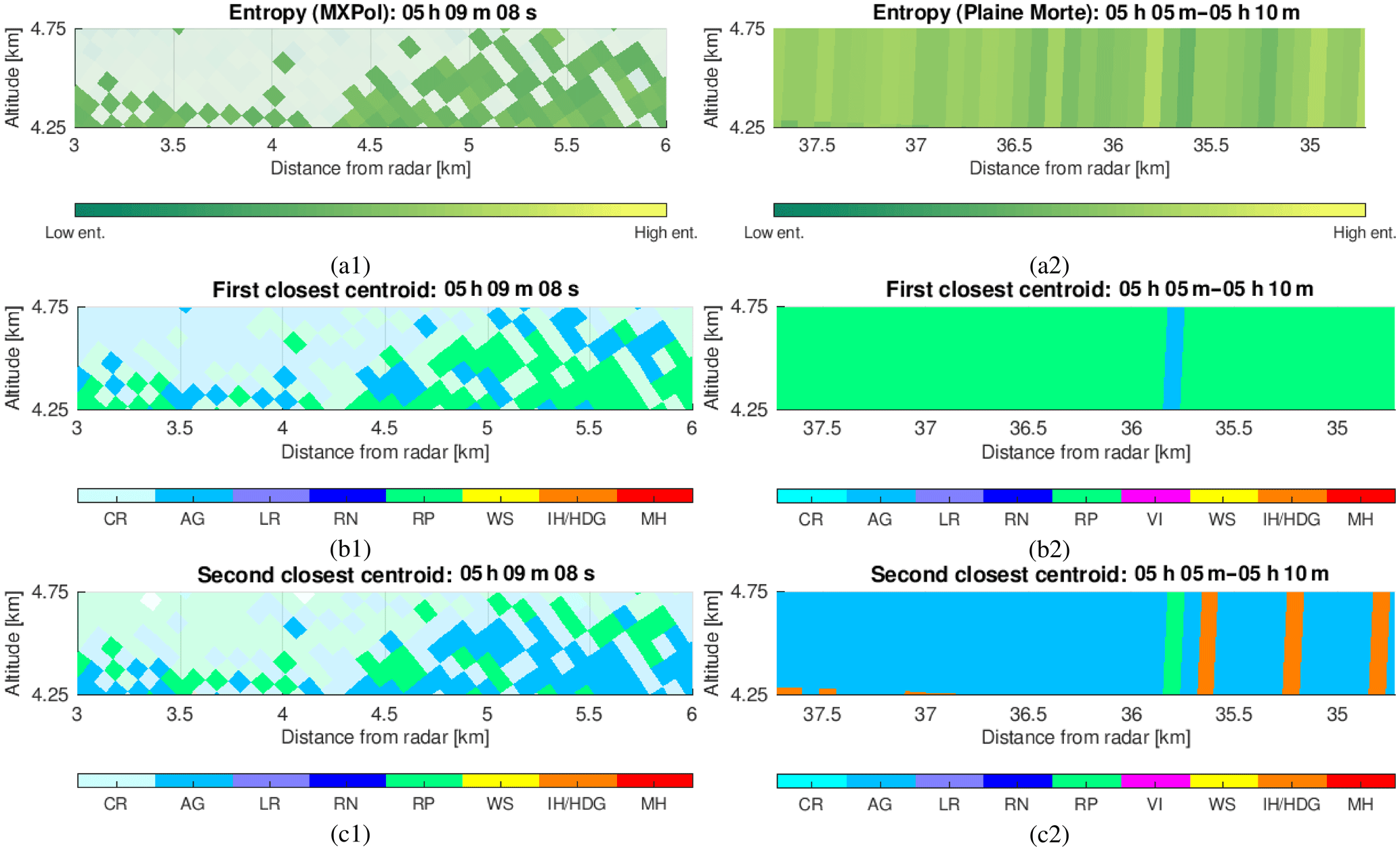
Figure 16 The example of (1) MXPol radar RHI and (2) Plaine Morte reconstructed RHI (from the dataset used in Sect. 3), with the accentuated volumes with entropy H>0.4: (a) the entropy of the region of interest, (b) the first-closest centroid, (c) the second-closest centroid .

In Fig. 16a we see the region of significant transitions between aggregates and rimed ice particles, seen simultaneously by the MXPol and the Plaine Morte radar, which is, due to the entropy estimation (thresholded at H>0.4), suspected to be dominated by mixtures. The subsequent Fig. 16b and c show the first (the closest centroid) and the second (the second closest centroid) dominant component as seen by the hydrometeor classification. Rather than analyzing separately each of the pixels and estimating the proportions of these components by applying the bin-based approach based on the assumption of coherence, here we analyze the potential of the PCA and ICA techniques to detect the potential residual incoherency. That is to say, we try to infer either the coherent component or the component cleaned of any interferences,involved in the overall mixing process, by considering the ensemble of the pixels, regardless of their position in space.

We start by taking all the pixels observed by the MXPol radar in one of the acquisitions during the extended event introduced in Sect. 3.1.2 (34 acquisitions between 4:00 and 6:00 UTC on 28 February 2017) and characterized by higher entropy values (H>0.4). By representing them in a space formed by our four transformed and stretched polarimetric variables, we obtain a not exactly informative cloud of points (black circles in Fig. 17). This cloud of points, which would be the matrix X introduced in Eq. (11) (each point is a matrix column), is characterized by relatively high entropy values, as this was the criterion for the selection of the region of interest. The following four columns in Fig. 17 represent the vectors k_i, which are the axes of the new space, i.e., the principal, uncorrelated components (in blue), or the independent components (in red).

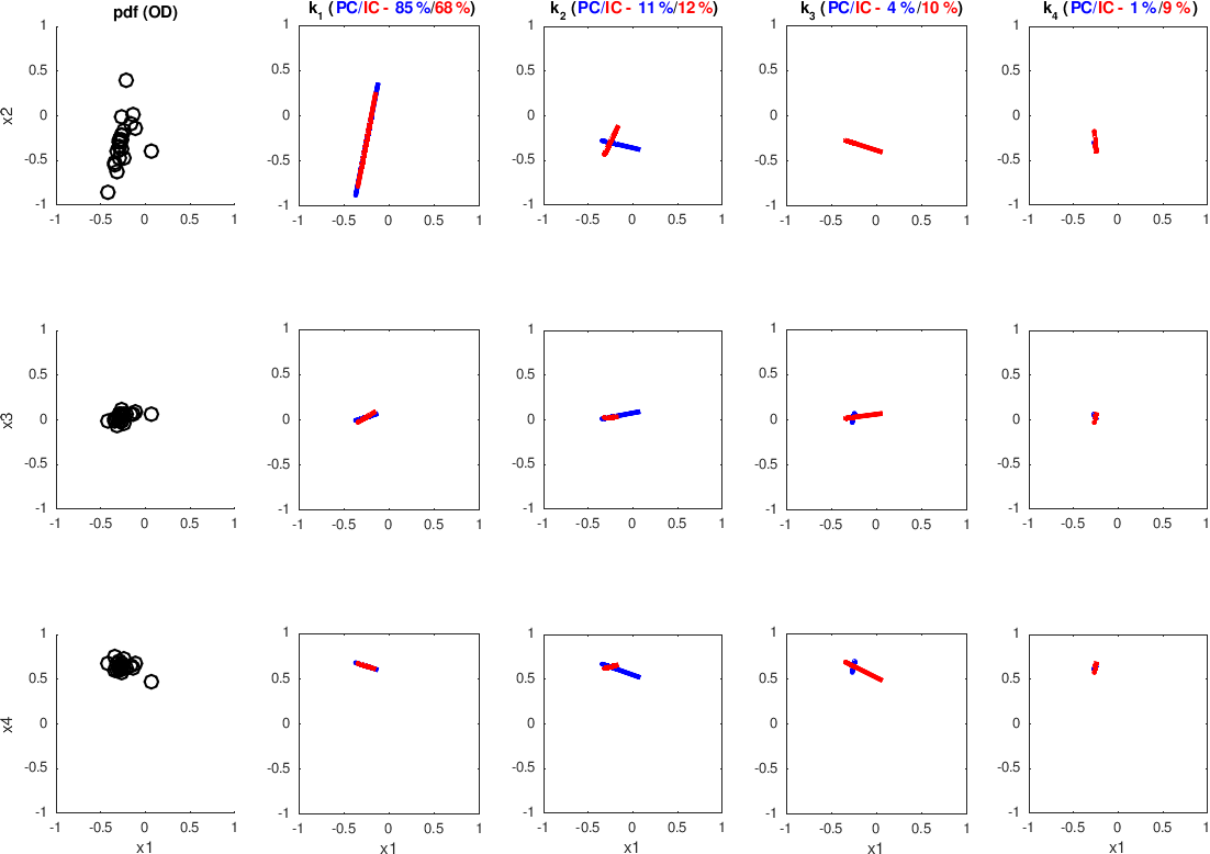
Figure 17 PCA (blue) and ICA (red) applied to the H>0.4 regions of an example of the RHI from the event considered in the inter-radar comparison in Sect. 3.1 (MXPol X-band data).

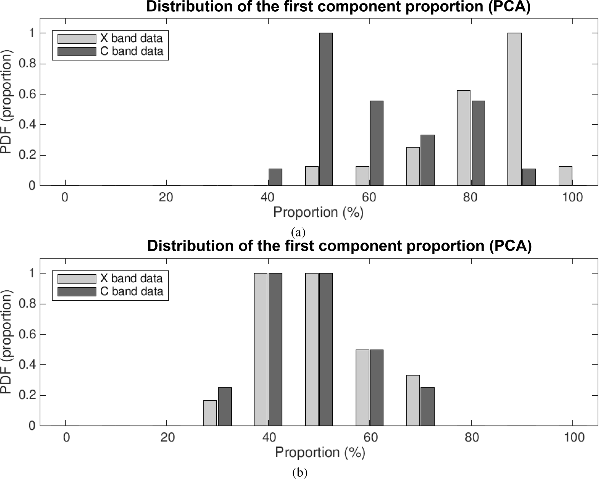
As suggested in Sect. 4.1, the first uncorrelated component is supposed to represent a pure component, freed up of the effect of incoherency in the data acquisition. And indeed, this first component does cover the majority of spatial variance (in Fig. 17, the proportion of the first component is about 85 % for the PCA and 68 % for the ICA), indicating that we should not be too concerned by the residual incoherency. It is even truer if we recall that our sample cannot be considered as completely homogeneous, meaning that the portion of variance unexplained by the first uncorrelated component does not exclusively refer to the incoherency. By repeating the analysis over the entire considered event, we confirm that the proportion of the first component is important enough to discard a significant influence of residual backscattering incoherency (Fig. 18a), its median value being 86 % and its median Cloude and Pottier entropy value (Eq. 3, with λ_i from Eq. 10 taking the role of p_i) being ${\stackrel{\mathrm{̃}}{H}}_{\mathrm{CP}}=\mathrm{0.38}$. The low value of H_CP emphasizes the non-uniform distribution among proportions of the four estimated principal components.

Figure 18 The distribution of the proportions of the most dominant component, calculated by generalizing the analysis illustrated in Figs. 16, 17 and 19 onto the entire (extended) event considered in the inter-radar comparison in Sect. 3.1: (a) PCA, (b) ICA.

Unfortunately, by evaluating the entropy estimate of the pure component in the space of the original centroids, we see that these vectors k_i do not correspond at all to the predefined centroids (not illustrated in Figs. 17 and 19). Hence, they cannot be considered at all as the pure components in the context of the hydrometeor classification. The conclusion is confirmed by checking the entropy distribution of the proportions of original data contributing to each of the components (Eq. 12). This implies that PCA cannot really be used as a de-mixing tool, because the coherent backscattering proportion corresponds not to the backscattering of a pure hydrometeor type but rather to the backscattering of the mixture.

Aside from uncorrelated components, in Fig. 17, we also show the results of employing the introduced FastICA method (with kurtosis value for the measure of non-Gaussianity), following its demonstrated benefits in the framework of the SAR decomposition theory (Besic et al., 2015; Pralon et al., 2016). The principal advantage of this tool with respect to PCA would be the lack of the orthogonality constraint. Basically, each successive component is not required to be orthogonal to the previous one but is the one which is genuinely independent, assuming the very plausible non-Gaussianity of the data. This effect, allowing for the subtle “splitting” of the first component, causes the proportion of the first estimated component, event though it obviously corresponds to the first uncorrelated component, to end up being far inferior with respect to the one estimated by PCA (over the entire event, median proportion of 46.4 % and ${\stackrel{\mathrm{̃}}{H}}_{\mathrm{CP}}=\mathrm{0.86}$, with p_i being $\left|\right|{\mathit{k}}_{\mathrm{1}}|{|}_{\mathrm{2}}^{\mathrm{2}}$). This kind of increased sensibility, which results in the subtle splitting of the first component, does not indicate higher incoherency than seen by PCA but rather confirms the previously stated assumption that the incoherence is not the dominant cause of the proportion unexplained by the first correlated component.

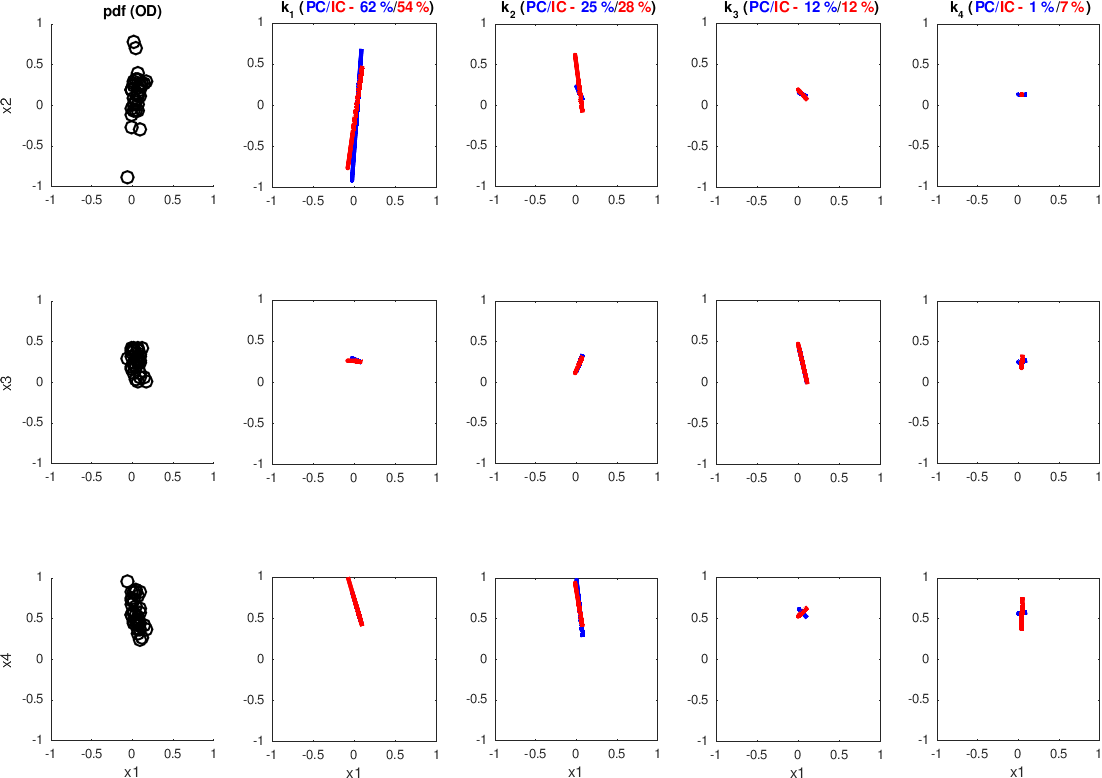
Figure 19 PCA (blue) and ICA (red) applied to the H>0.4 regions of an example of the RHI from the event considered in the inter-radar comparison in Sect. 3.1 (Plaine Morte C-band data).

The same analysis applied to the Plaine Morte data (24 acquisitions between 4:00 and 6:00 UTC on 28 February 2017) is illustrated in Fig. 19. The quantitative parameters estimated over the entire event (PCA: median proportion of the first component, 56 %, ${\stackrel{\mathrm{̃}}{H}}_{\mathrm{CP}}=\mathrm{0.73}$; ICA: 46.4 %, ${\stackrel{\mathrm{̃}}{H}}_{\mathrm{CP}}=\mathrm{0.88}$) show a drop in the first uncorrelated component proportion (Fig. 18), a drop which can be explained by the significantly increased volume size (which can be seen in Fig. 16) and a lower number of pulses averaged in estimating the polarimetric parameters. Both factors logically make the hypothesis of negligible random interference slightly weaker.

Aside from studying the potential effect of incoherency, this analysis is also useful in highlighting the limit of the concept of discrete hydrometeor classification. Namely, this concept prevents us from exploiting the conventional tools in dealing with the residual incoherency that could allow us to have an even more systematic and assumptions-free insight into the mixed-radar sampling volumes, with respect to the one presented in this article as the bin-based approach. A possible way forward would be to investigate the possibility of modeling the weather radar target vector. Following suggestions from the micro-physical modeling community (Morrison and Milbrandt, 2015) or practices from the SAR remote-sensing community (Touzi, 2007), one could develop a way to introduce some degrees of liberty in depicting hydrometeor classes, degrees of freedom which would reflect the physical properties of the hydrometeor itself. That would not guarantee that we would exploit all the statistical information from the measurements, because inferring total independence might not even be possible (the proportions summing up to unity could represent an obstacle to the concept of independence, as suggested by Nascimento and Dias, 2005). However, it could very probably allow us to account for the incoherency by exploiting the first two statistical moments (PCA).

5 Conclusions and future perspectives

In this paper, we address the issue of hydrometeor mixtures in polarimetric radar measurements by adapting the paradigm of decomposition/unmixing widely elaborated in other remote-sensing domains to the field of weather radar remote sensing.

In the first part of the paper we propose a bin-based de-mixing approach, which is largely based on the hypothesis of coherent backscattering of hydrometeors inside the radar sampling volume. The proposed approach is built upon the semi-supervised hydrometeor classification method which reduces the classification problem to the distances in the Euclidean space formed essentially by the polarimetric parameters (Besic et al., 2016) but could be adapted to any classification technique providing a distance to the various hydrometeor types. Inspired by the SAR polarimetric decomposition on standard mechanisms and hyperspectral linear unmixing, the method estimates proportions of different hydrometeor classes in each radar sampling volume, without considering the wider spatial context. The performance of such an approach is analyzed in three stages, based on C-band and X-band radar data, together with a ground-based Multi-Angle Snowflake Camera. The analysis, aside from demonstrating the potential of the method, also shows the improved matching between different radars and, most significantly, the improved matching between the radar and the independent ground-based instrument.

The second part of the paper is dedicated to the study of a potential influence of the residual spatial incoherency in the backscattering of hydrometeors inside the radar sampling volume. The study is based on adapting the conventional statistical methods, such as PCA and ICA, used to deal with the spatial incoherency in the SAR remote sensing to the specific framework of the weather radar polarimetry. The performance analysis points out the limited influence of the residual incoherency in the regions of hydrometeor mixtures. The introduced evaluation of the spatial consistency in the case of heterogeneousness radar sampling volumes is important given that potentially present incoherency is not only due to the intraclass variability but also due to the interclass hydrometeor variability. The conclusion, implying that after all there is not a significant rise in incoherency in the case of hydrometeor mixtures on the one hand strengthens the proposed bin-based approach and on the other hands makes the tools such as PCA and ICA less useful in the context of weather radar decomposition/de-mixing than they are in the context of SAR remote sensing.

The overall message of this paper is to focus some attention of the weather radar community on the importance of the decomposition/de-mixing methods, which make it possible to look into the radar sampling volume. The present work remains exploratory, and many avenues still need to be explored, including the potential benefits of a continuous hydrometeor classification approach. Finally, the proposed bin-based approach, allowing already plausible and fairly validated estimation of hydrometeor type at the sub-bin level, can be used to improve the quantitative estimation of precipitation using radar.