the Creative Commons Attribution 4.0 License.
the Creative Commons Attribution 4.0 License.
 | 24 Aug 2018
Comparison study of COSMIC RO dry-air climatologies based on average profile inversion
Marc Schwärz
Veronika Proschek
Ulrich Foelsche
Hans Gleisner
Global Navigation Satellite System (GNSS) radio occultation (RO) data enable the retrieval of near-vertical profiles of atmospheric parameters like bending angle, refractivity, pressure, and temperature. The retrieval step from bending angle to refractivity, however, involves an Abel integral with an upper limit of infinity. RO data are practically limited to altitudes below about 80 km and the observed bending angle profiles show decreasing signal-to-noise ratio with increasing altitude. Some kind of high-altitude background data are therefore needed in order to perform this retrieval step (this approach is known as high-altitude initialization). Any bias in the background data will affect all RO data products beyond bending angle. A reduction of the influence of the background is therefore desirable – in particular for climate applications.
Recently a new approach for the production of GNSS radio occultation climatologies has been proposed. The idea is to perform the averaging of individual profiles in bending angle space and then propagate the mean bending angle profiles through the Abel transform. Climatological products of refractivity, density, pressure, and temperature are directly retrieved from the mean bending angles.
The averaging of a large number of profiles suppresses noise in the data, enabling observed bending angle data to be used up to 80 km without the need for a priori information. Some background information for the Abel integral is still necessary above 80 km.
This work is a follow-up study, having the focus on the comparison of the average profile inversion climatologies (API) from the two processing centers WEGC and DMI, which study monthly COSMIC (Constellation Observing System for Meteorology, Ionosphere, and Climate) data from January to March 2011. The impact of different backgrounds above 80 km is tested, and different implementations of the Abel integral are investigated. Results are compared for the climatological products with ECMWF analyses, MIPAS, and SABER data.
It is shown that different implementations of the Abel integral have little impact on the API climatologies. On the other hand, different extrapolations of the bending angle profile above 80 km play a key role in the resulting monthly mean refractivities above 35 km in altitude. Below that respective altitude the API climatologies show a good agreement between the two processing centers WEGC and DMI. Due to the downward propagation within the retrieval, effects of the high-altitude initialization lead to differences in dry-temperature climatologies down to 20 km in altitude.
When applying an exponential extrapolation to the bending angles above 80 km at both centers, the dry-temperature climatologies agree among WEGC, DMI, ECMWF analysis, and MIPAS up to 35 km in altitude within ±0.5 K and up to 40 km in altitude within ±1 K. We conclude that the API retrieval is a valid approach up to the lower stratosphere. It is a computationally efficient alternative method for producing dry atmospheric RO climatologies.
- Article
(3607 KB) - Full-text XML
- BibTeX
- EndNote


The Global Navigation Satellite System (GNSS) radio occultation (RO) technique (Anthes, 2011; Kursinski et al., 1997; Steiner et al., 2001) is accepted as a valuable data source for numerical weather prediction (NWP) and climate monitoring, in particular in the upper troposphere and lower stratosphere (UTLS). The altitude range from 5 to 35 km is commonly known as the core region of the RO technique. Due to their high accuracy, RO data have significantly reduced systematic errors in global weather analyses (Cardinali, 2009; Healy and Thépaut, 2006) and their potential for climate monitoring has been demonstrated with simulation studies (Foelsche et al., 2008b; Leroy et al., 2006; Ringer and Healy, 2008) and analyses (Foelsche et al., 2008a, 2009; Ho et al., 2012; Steiner et al., 2013).
At most NWP centers, RO data are assimilated in the form of bending angles. Climate monitoring based on RO data, on the other hand, requires the full range of geophysical parameters, from refractivity via density and pressure to temperature, since the geophysical variables change differently in different parts of the atmosphere (Foelsche et al., 2008b), and temperature data are desired for comparison with data from other sources.
RO climatologies from different satellite missions like Challenging Minisatellite Payload (CHAMP) and Constellation Observing System for Meteorology, Ionosphere, and Climate (COSMIC) are very consistent (within 0.05 %) up to 30 km in altitude (temperature) and 35 km in altitude (refractivity) when the same retrieval scheme is used for all data (Foelsche et al., 2011). Data processed from different centers show differences due to structural uncertainty, which is still small at the bending angle level but increases through the retrieval chain (Ho et al., 2012; Steiner et al., 2013). The retrieval step from bending angle to refractivity is a major source for structural uncertainty, because it requires background information at high altitudes, where individual RO profiles are too noisy. When the observations and background are combined by statistical optimization, the observations are inversely weighted with the assumed measurement error. A bias in the background profile will result in a bias in the retrieved profile down to an altitude that depends on the noise of the data. The hydrostatic integral in the retrieval step from density to pressure will also lead to a further downward propagation of potential biases in background data. An unbiased high-altitude background – or data with low noise up to high altitudes – would therefore be highly beneficial.
Ao et al. (2012) and Gleisner and Healy (2013) suggested that the impact of high-altitude background information could be reduced in climate applications when averages over many RO profiles are used. In both studies average refractivity profiles have been obtained by averaging many COSMIC bending angle profiles in a domain and then inverting this average bending angle profile to a single refractivity profile (instead of averaging refractivity profiles, which have been obtained by inverting individual bending angle profiles). Danzer et al. (2014) successfully applied this average profile inversion approach (API) to CHAMP data, which are more challenging due to their higher noise level. Scherllin-Pirscher et al. (2015) introduced an alternative approach, wherein averaged COSMIC profiles are used to build a bending angle climatology up to high altitudes, which can then be used as the background for the retrieval of individual profiles.
The advantages of the API approach are the following: (a) the reduction of background in the data, (b) the circumvention of the complicated statistical optimization step (a known reason for differences between processing centers), and (c) the API approach is a much faster computation.
In this study, we test different implementations of the API approach at the Danish Meteorological Institute (DMI) and the Wegener Center for Climate and Global Change (WEGC) and validate them both against independent data. We analyze 3 COSMIC test months from January to March 2011, following the investigations of Gleisner and Healy (2013). A long-term API data set study has already been performed for the complete CHAMP period (Danzer et al., 2014), and it is not part of this investigation. The aim of the API approach is to produce high-quality climatologies with well-characterized errors, which might push current limits in altitude further upwards, enabling the study of stratospheric climatologies above 35 km.
The structure of this paper is as follows: Sect. 2 explains the method and the different implementations at WEGC and DMI. Section 3 describes the data set, and Sect. 4 shows results from the comparison climatologies obtained by API and (traditionally) by averaging individual profiles obtained by single-profile processing. In Sect. 5 we compare the different API implementations and validate them against data from MIPAS (Michelson Interferometer for Passive Atmospheric Sounding) and SABER (Sounding of the Atmosphere using Broadband Emission Radiometry), and against European Centre for Medium-Range Weather Forecasts (ECMWF) analyses, followed by a summary and conclusions in Sect. 6.
The retrieval step from bending angle profiles to refractivity profiles uses an Abel transform, which relates the refractive index n to the bending angle α:
where a is the impact parameter and x=nr, with r being the radius vector of a point on the ray path. The Abel integral to infinity raises a problem, since RO data are practically limited in altitude to about 80 km. Furthermore, the observed bending angle profiles suffer from a decreasing signal-to-noise ratio with increasing altitude. The need for an extrapolation step together with the handling of the noisy bending angles requires a high-altitude initialization. This is performed at most of the RO processing centers through a statistical optimization step (SO), where observations and background information are combined and are weighted inversely with the respective error statistics (for details of different implementations see Ho et al., 2009, 2012). Different processing centers use different kinds of background information (e.g., from climatological models such as Mass Spectrometer and Incoherent Scatter Radar (MSIS), or meteorological data such as ECMWF analysis) and different implementations of the statistical optimization step (Gobiet and Kirchengast, 2004; Gorbunov, 2002; Lohmann, 2005).
The basic idea of the API approach is that averaging of the data in bending angle space suppresses the noise in the data, so that the observed bending angle can be used up to 80 km and the SO step becomes largely obsolete. Above 80 km the bending angle still needs to be extended, because the Abel integral upper limit is infinity and the bending angle is not zero above 80 km. Different extrapolations of the bending angle are tested in this study, as described in Sect. 2.1 and 2.2
The main steps of the API retrieval can be summarized as (a) a generation of the average bending angle as a function of impact altitude, (b) change of height variable from impact altitude to impact parameter, a, using an average radius of curvature, , (c) extrapolation of the average bending angle profiles to infinity, which we introduce as high-altitude extrapolation, (d) retrieval of the average refractivity as a function of x=nr using the Abel transform (Eq. 1), and (e) change of height variable to mean sea level altitude using the same radius of curvature as in step (b). For details see Danzer et al. (2014); Gleisner and Healy (2013).
2.1 WEGC implementation
The latest implementation of the inversion of the individual profiles at WEGC is currently in an experimental state. It is based on the so-called base-band method (Kirchengast et al., 2016, 2017). Excess phase profiles provided by the COSMIC Data Analysis and Archiving Center (CDAAC) of the University Corporation for Atmospheric Research (UCAR), Boulder, Colorado were used as input data. From these data bending angle profiles are calculated by applying a combined geometric optics (see Appendix A in the study by Schwarz et al., 2018) and wave optics (Gorbunov and Kirchengast, 2018; Gorbunov and Lauritsen, 2004) bending angle retrieval. To obtain ionosphere-free bending angles, the method by Sokolovskiy et al. (2009) is applied on the calculated bending angles. Each bending angle profile is then statistically optimized using an ECMWF short-range bias-corrected forecast as background profile (Li et al., 2013, 2015). The refractivity is then calculated, applying the method described by Syndergaard and Kirchengast (2016) in Appendix B. Dry pressure and dry temperature are obtained by computing the hydrostatic integration (once more on the residual state, cf., Appendix A by Schwarz et al., 2017). The monthly climatologies are then obtained by averaging the individual profiles into latitude bins.
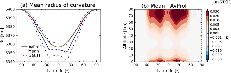
The API processing at WEGC follows the basic description given in Sect. 2. The mean, median, and so-called medmean bending angle climatologies are calculated. Medmean uses mean bending angle values below 50 km, median values above 60 km, and a linear combination in between (Gleisner and Healy, 2013). Together with the average bending angles, the average radii of curvature are built, where we test three different implementations of mean (see Eqs. 2–4, and Fig. 1). The first formulation of follows Gleisner and Healy (2013) and is determined as the sum of all single radii of curvature per bin (Rc,i with occultation i) divided by the number of occultations m in a bin:
As an alternative formulation we test the Earth's mean radius of curvature at latitude φ:
with ,
and N(φ)=
, a is the Earth's
equatorial radius of 6 378.1370 km, and b is the Earth's polar radius
of 6 356.7523 km (WGS84, World Geodetic System, 1984). Furthermore, we
study the formulation of Earth's Gaussian radius of curvature at latitude
φ (Torge, 2001):
The left panel of Fig. 1 compares the mean radius of curvature using the three different formulations of (Eq. 2 to Eq. 4), studying monthly 5∘ zonal COSMIC data from January 2011. Obviously, the mean (green line) and the Gaussian (red dashed line) show almost no differences (Eqs. 3 and 4, respectively). Compared to the average per bin (Eq. 2, AvProf shown by the blue line, its standard deviation shown by the blue dashed line) differences increase in the tropics between about 2 and 8 km. The reason is that the local radius of curvature in north–south (meridian) direction, i.e., M(φ), and the local radius of curvature in east–west (normal to meridian) direction, i.e., N(φ), show maximum differences at the equator, while at the poles they are equal. When building a mean , M(φ) and N(φ) were either averaged by using the mean or the Gaussian formula (Eqs. 3 and 4). In case of a single RO measurement, the radius of curvature is computed for the GNSS and low Earth orbit (LEO) satellite orbits at a given time. Using as a third formulation, a simple averaging of all radii of curvature in a bin, we therefore find the largest differences between ±30∘ latitude (see left panel of Fig. 1). However, the impact of the different formulations of on the dry temperature was found to be negligible in the stratosphere; see right panel of Fig. 1. The variations are between about 0.001 K to about a few 0.01 K up to 80 km in altitude, comparing the same monthly 5∘ zonal (5∘ latitude × 360∘ longitude) COSMIC climatology.
Different high-altitude extrapolations above 80 km have been tested. Initially we study monthly means of ECMWF analysis fields converted to refractivity, as values for the Abel integral from infinity to 80 km (Kirchengast et al., 2017). These data sets are labeled “fulltop”. As an alternative, an exponential extrapolation of the bending angles to infinity is tested (exptop), where scale height and fitting coefficient are calculated from a log-linear fit to each average bending angle profile. Furthermore, the case of setting the average bending angles to zero above 80 km is studied (notop). Additionally a sensitivity study from the fulltop value to notop in incremental steps of 1∕5 is performed (notop =0, top1 fulltop, top2 fulltop, top3 fulltop, top4 fulltop, fulltop). For an overview of all data sets, see Table 1.
Finally the average bending angles are propagated through the Abel integral using the base-band method, and they are then processed as described for the individual profile processing at WEGC.
2.2 DMI implementation
The DMI data based on the standard IPI processing were obtained from a reprocessed climate data record provided by the Radio Occultation Meteorology Satellite Application Facility (ROM SAF), which is a decentralized RO SAF under the European Organisation for the Exploitation of Meteorological Satellites (EUMETSAT). The ROM SAF COSMIC data are based on input data from the CDAAC/UCAR archive. The individual bending angle profiles are calculated using a combination of geometric optics and wave optics approaches, followed by smoothing and merging with a background profile taken from the BAROCLIM climatology (Scherllin-Pirscher, 2013; Scherllin-Pirscher et al., 2015). The statistical optimization step is followed by an Abel transform, to retrieve the refractivity profile, and a hydrostatic integration, to retrieve the dry-temperature profile (Lauritsen et al., 2011). The monthly climatologies are then obtained by averaging the individual profiles into latitude bins.
The API processing used by DMI in the present study is described in more detail by Gleisner and Healy (2013). The average bending-angle profiles are computed as a combination of mean (below 50 km), median (above 60 km), and a linear combination of the two (from 50 to 60 km). The statistical analysis is done on a common impact altitude grid, which is mapped to an impact parameter grid using an average radius of curvature, , according to Eq. (2). This is followed by an extrapolation of the average bending angle profile from the top of the profile up to infinity assuming a constant scale height of 7.5 km, in contrast to WEGC, which calculates the scale height individually for each mean bending angle. The exponential extrapolation of the bending angles is called “exptop” in the data sets. The Abel transform (Eq. 1) is then used to retrieve refractivity as a function of x=nr, which is mapped to mean-sea level altitude, H, using the mean radius of curvature, .
In the present study, DMI used an implementation of the Abel transform provided by the ROM SAF Radio Occultation Processing Package (ROPP) (Culverwell et al., 2015). This assumes that the bending angle, α, can be approximated as a linear function of impact parameter, a, between successive grid points. The sub-integrals between the grid points can then be solved analytically, and the refractivity at a certain height, x, is simply given by a sum of the contributions from the atmospheric layers from height x to the top of the atmosphere.
We analyze occultations from the six-satellite mission Formosa Satellite Mission 3/COSMIC (F3C) for the year 2011, from January to March. Excess phase profiles and precise orbit information were retrieved from the UCAR/CDAAC database and then further converted into bending angle profiles and dry-air profiles (referred to as level L2a processing) at the WEGC and also at the DMI, using the rOPS-ex (reference Occultation Processing System-experimental) and ROPP version 8, respectively. We call the processing chain of a single bending angle profile to dry temperature the individual profile inversion (IPI). In the next step, the profiles were binned into monthly 5∘ zonal climatologies (IPI climatologies) at both processing centers.
The WEGC and DMI API climatologies were produced using the same COSMIC data sets as described in Sect. 2. The API climatologies are available for bending angle, refractivity and dry temperature (L2a processing) on a monthly 5∘ zonal grid. At the WEGC, the API climatologies were produced using processing routines from rOPS-ex (Abel inversion, hydrostatic integral), and at the DMI, ROPP processing routines were used. We tested different high-altitude extrapolations in the API processing (see description in Sect. 2). An overview of the data sets and all data versions (fulltop, exptop, etc.) is given in Table 1. To aid clarity, we give two examples.
The label “WEGC (L1b DMI) – fulltop” refers to an input bending angle climatology generated at the DMI (Gleisner and Healy, 2013), hence “L1b DMI”, and then forwarded through processing routines from WEGC using the WEGC high-altitude extrapolation fulltop. On the other hand, “DMI (L1b DMI) – exptop” uses the same bending angle input climatology from the DMI but produces the climatology with the DMI processing routines, using the exptop high-altitude extrapolation. So, in summary, those two processing versions share the same input bending angle climatology but differ in processing (WEGC and DMI) and in their handling of the extrapolation (fulltop and exptop).
Table 1Data sets from the COSMIC mission, always for monthly 5∘ zonal climatologies of the dry atmosphere.
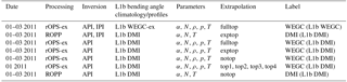
Table 2Reference data sets for Table 1 on monthly 5∘ zonal climatologies.
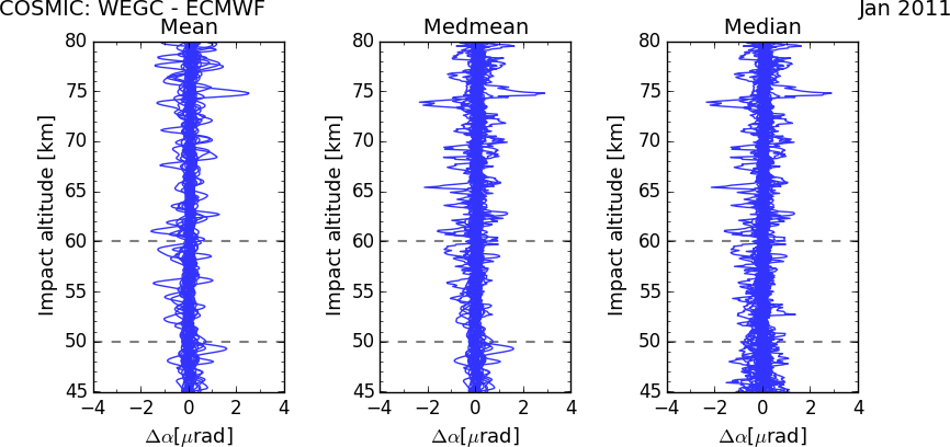
Figure 2L1b WEGC: bending angle difference of mean, medmean, and median relative to ECMWF analyses for January 2011.
As reference data sets, co-located profiles from ECMWF analysis data were studied on 5∘ latitudinal bins. The analysis data fields were used at a T42L91 resolution, since the T42 horizontal resolution matches the horizontal resolution of RO data (∼300 km). The ECMWF analysis climatologies were used as reference data sets from the bending angle down to temperature (i.e., Level L2a climatologies); see Table 2.
We also use data from the MIPAS and SABER instruments as reference data sets. The MIPAS instrument, on board Environmental Satellite (ENVISAT), operated from July 2002 to April 2012, providing global temperature, pressure, and trace gas observations in an altitude range from about 6 to 70 km. SABER, on board the Thermosphere Ionosphere Mesosphere Energetics and Dynamics (TIMED) satellite, measures data since 2001, providing temperature, pressure, density, geopotential height, and trace species. The coverage is nearly global, between 52∘ S–82∘ N and 82∘ S–52∘ N, respectively, alternating every 2 months and providing a continuous coverage from 52∘ S–52∘ N in an altitude range from about 10 to 180 km. A validation study of MIPAS temperature in the middle atmosphere showed good agreement with SABER temperature (<0.5 K) at midlatitude in the upper troposphere (García-Comas et al., 2012).
Innerkofler (2015) carried out a profile to profile intercomparison study between WEGC RO OPSv5.6 data and ECMWF, MIPAS, and SABER data. The study shows good agreement between ECMWF analyses and RO data up to 80 km, with temperature differences of about ±1 K. MIPAS data also show good agreement up to 40 km in altitude with differences of about ±1 K. Between 40 and 50 km height these differences increase to about ±2 K. In contrast to MIPAS, SABER data show a cold bias of 3 K between 20 and 35 km. From 35 to 45 km in altitude the differences decrease to ±2 K.
We start our analysis with the investigation of API climatologies from WEGC. API climatologies have already been thoroughly tested at the DMI (Danzer et al., 2014; Gleisner and Healy, 2013), showing very good agreement between API and IPI refractivity climatologies up to 35 km in altitude.
Initially, we investigate monthly 5∘ zonal rOPS-ex bending angle climatologies (WEGC L1b) for the COSMIC satellite mission for January 2011. Figure 2 shows the differences of the mean, medmean, and median bending angles relative to co-located ECMWF analyses. The dashed grey lines mark the transition region of the medmean bending angles. Obviously the bending angles show strong variations relative to ECMWF analyses. We emphasize that those bending angles are only recently generated experimental data, which is one reason why we later continue our analysis based on DMI bending angles.
As a next step we compare API to IPI climatologies using the rOPS-ex bending angles (WEGC L1b) as input for the API and IPI processing. All refractivity differences are studied as relative differences given as a percentage, while the temperature differences are given in Kelvin. Figure 3 shows the difference between API and IPI refractivity (left column) and dry-temperature (right column) climatologies, from January to March 2011 (top to bottom). In analyses of the refractivity differences, the API and IPI climatologies show almost identical results up to 40 km in altitude. The largest differences are around the tropopause, and in the height range between 40 and 50 km, and they vary between about 0.2 % and 0.6 %. This confirms the results from previous studies, that the API method is a valid alternative to the IPI approach, since no significant differences are introduced.
The API and IPI dry-temperature climatologies agree within the RO core region of 35 km in altitude (lower stratosphere) very well. Above 35 km, differences start to increase by about 1 K every 3 to 5 km in altitude.
Summarizing the main results from this analysis: first, it was possible to successfully implement the API approach at the WEGC, as has been done in previous studies at the DMI. Second, the API approach does not introduce major differences within the RO core region of 10–35 km. Hence, it is a valid alternative for climate analysis in the lower stratosphere.
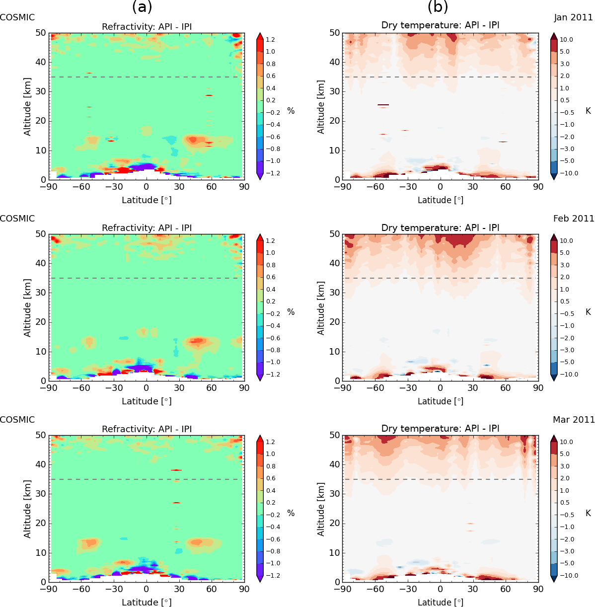
Figure 3WEGC: difference between API and IPI climatologies, analyzed for refractivity (a) and dry temperature (b), using L1b WEGC bending angles as input, studied from January to March 2011 (top to bottom).
The main focus of this study is a thorough comparison of API climatologies from the WEGC and DMI. Since we want to understand how differences enter the processing from API bending angle climatologies to refractivity climatologies, we decided to always use the same input bending angle climatology for both processing systems. For practical reasons we chose to study bending angle climatologies from the DMI, labeled DMI L1b, since WEGC rOPS-ex is still in development (see Fig. 2). Figure 4 shows the monthly 5∘ zonal mean, medmean, and median bending angle climatologies relative to ECMWF analyses for January 2011. The February and March 2011 results are very similar, so we only present results for 1 month here.
In the Abel integral we use medmean bending angles, because the mean value suffers from large-scale wiggles at high altitudes (see discussions given by Gleisner and Healy, 2013; Danzer et al., 2014).
5.1 API refractivity climatologies
In this section. we show comparisons of API refractivity climatologies from the WEGC and DMI. In Fig. 5, we show the difference of API refractivity climatologies relative to co-located ECMWF analyses, from January to March 2011. The left column corresponds to WEGC processing, while the right column corresponds to the DMI processing routines. A striking feature is that the WEGC differences above 35 km (left column) are always much larger relative to ECMWF than the DMI results (right column). Below 35 km the results are in general very consistent between WEGC and DMI. However, in the tropopause region the WEGC data show a slight increase relative to ECMWF and compared to the DMI. Since both processing centers use the same input bending angle climatologies (DMI L1b), these differences can only enter through alternative handling of the extrapolation (fulltop and exptop) and in the implementations of the Abel integral. Note that the main focus of this study is the stratosphere and that we therefore show “dry” parameters, which are not fully adequate to characterize moist regions in the lower troposphere. Specifically the refractivity bias structure in the low and midlatitude troposphere in the lowest few kilometers relative to ECMWF is not caused by the API retrieval. It can also be seen for the IPI method (see Figs. 5, 6, 7 shown by Gleisner and Healy, 2013). However, the error at the lowest m 2 km is probably due to the use of a mean radius of curvature.
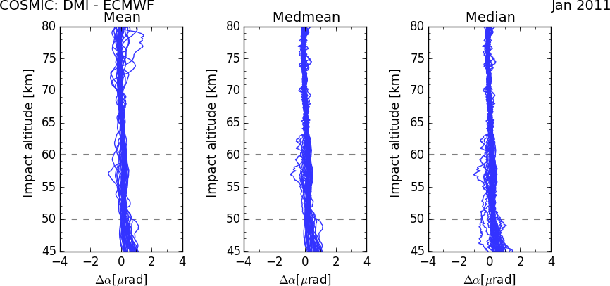
Figure 4DMI: bending angle difference of mean, medmean, and median relative to ECMWF analyses for January 2011.
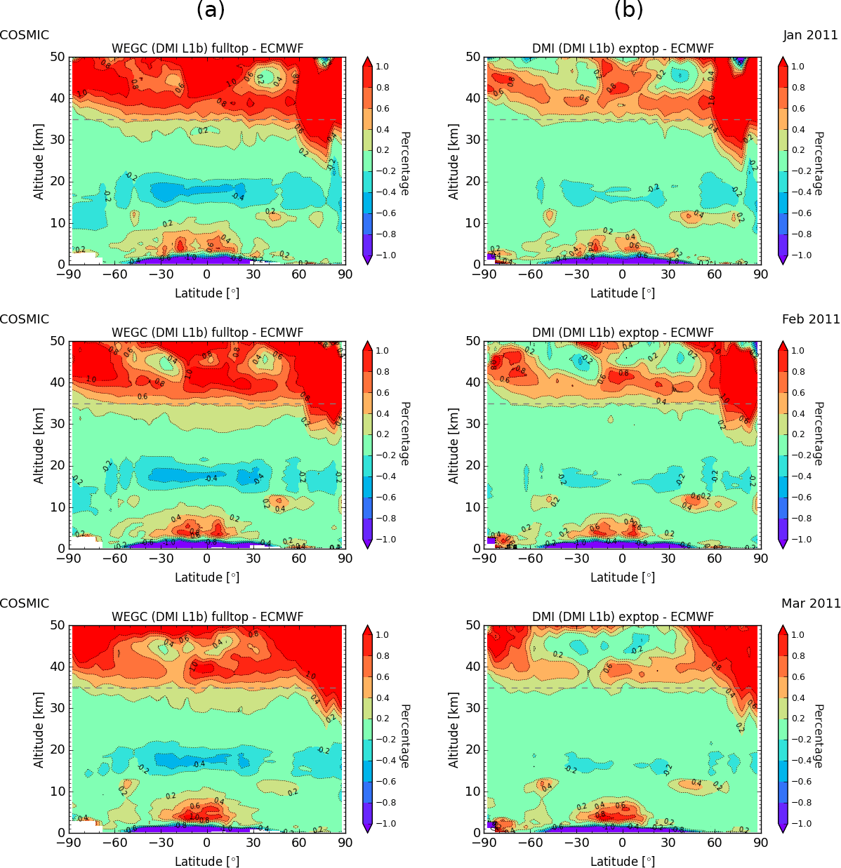
Figure 5API refractivity climatologies relative to ECMWF analyses, comparing WEGC processing (a) to DMI processing (b), from January to March 2011, using the same bending angle profiles as input (DMI L1b).
In order to illustrate the discrepancies between WEGC and DMI more clearly, Fig. 6 shows the differences between the two API climatologies. Clearly, the plot series confirms for all months that WEGC and DMI processing are almost identical up to 35 km, with the largest differences of 0.2 % in the tropopause region.
Nevertheless, we want to understand the occurring differences between WEGC and DMI, which is why we try to separate the underlying factors in the next two sections, i.e., the high-altitude extrapolation and the Abel integral.
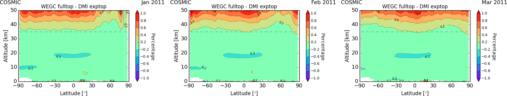
Figure 6Difference in API refractivity climatologies between WEGC and DMI processing from January to March 2011, using the same bending angle profiles as input (DMI L1b).
5.2 Testing the impact of the Abel integral
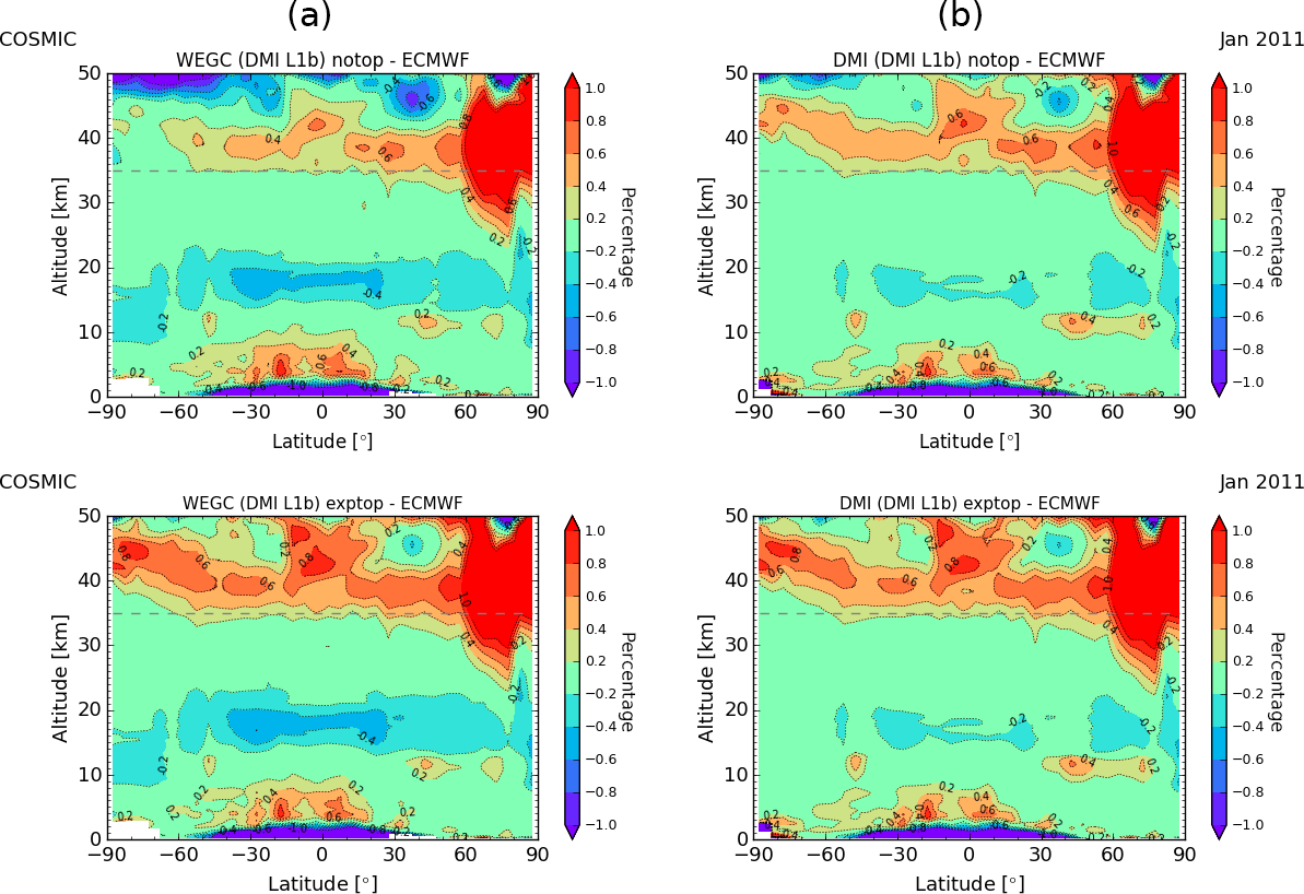
Figure 7API refractivity climatologies relative to ECMWF analyses, comparing WEGC processing (a) to DMI processing (b), for notop (first row) and exptop (second row), exemplary for January 2011.
Figure 7 shows the influence of different implementations of the Abel integral for January 2011. We also switch off the high-altitude extrapolation at both processing centers and set the bending angle climatologies to zero above 80 km (top row, notop), and initialize the bending angles at both centers with an exponential extrapolation (bottom row, exptop).
Clearly results show consistency between the two processing centers WEGC and DMI, once the high-altitude extrapolation is handled in the same way. Notop (first row) and exptop (second row) agree very well between WEGC and DMI, even above 35 km in altitude. However, there are small differences around the tropopause.
The discrepancies are more clearly illustrated by studying differences directly between WEGC and DMI (Fig. 8). The 0.2 % differences in the tropopause region are clear. Furthermore, we see that differences start to increase above 40 km with 0.2 % for the notop case (left plot). Almost identical results are found up to 50 km in altitude for the exptop case (right plot), with small exceptions in the high-altitude northern polar region. Since integration starts at 80 km in altitude only in the notop case, absolute values at 50 km are smaller than for the exptop case, and the same absolute difference corresponds to a higher relative difference. Hence differences begin to increase at 40 km in altitude for notop.
To sum up, these results suggest that the handling of the top has a significant influence on the API refractivity climatologies above 35 km. On the other hand, different implementations and discretizations of the Abel integral seem to lead to only small differences, mainly in the tropopause region. Hence we conclude that in the context of the API approach, a major focus should be on the handling of the bending angle profiles above 80 km.
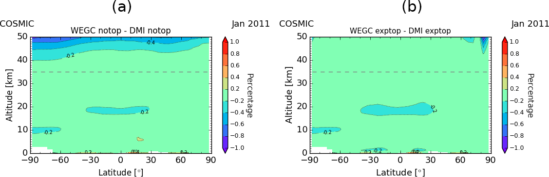
Figure 8Difference between WEGC and DMI API refractivity climatologies for notop (a) and exptop (b), exemplary for January 2011.
5.3 Testing the impact of different high-altitude extrapolations
This section presents a first attempt to address the high-altitude extrapolation. From the initial testing of the WEGC and DMI API processing, it is clear that the extrapolation approach has a substantial impact on the resulting refractivity climatologies above 35 km. The question of how to handle the extrapolation of the bending angles is of course a general question, and it also applies to individual profile processing. The rOPS-ex of WEGC is still in the development process, and this is an area of ongoing research.
In a first analysis we investigate the sensitivity of the API refractivity climatologies with respect to different top values for January 2011. We start in Fig. 9 from a top value of zero and increase the top value in incremental steps of 1∕5, until we reach the fulltop value of the rOPS-ex. Clearly, the results are insensitive to different top values below 35 km, while errors increase at 40 km already up to 1 % relative to ECMWF analyses for the fulltop value.
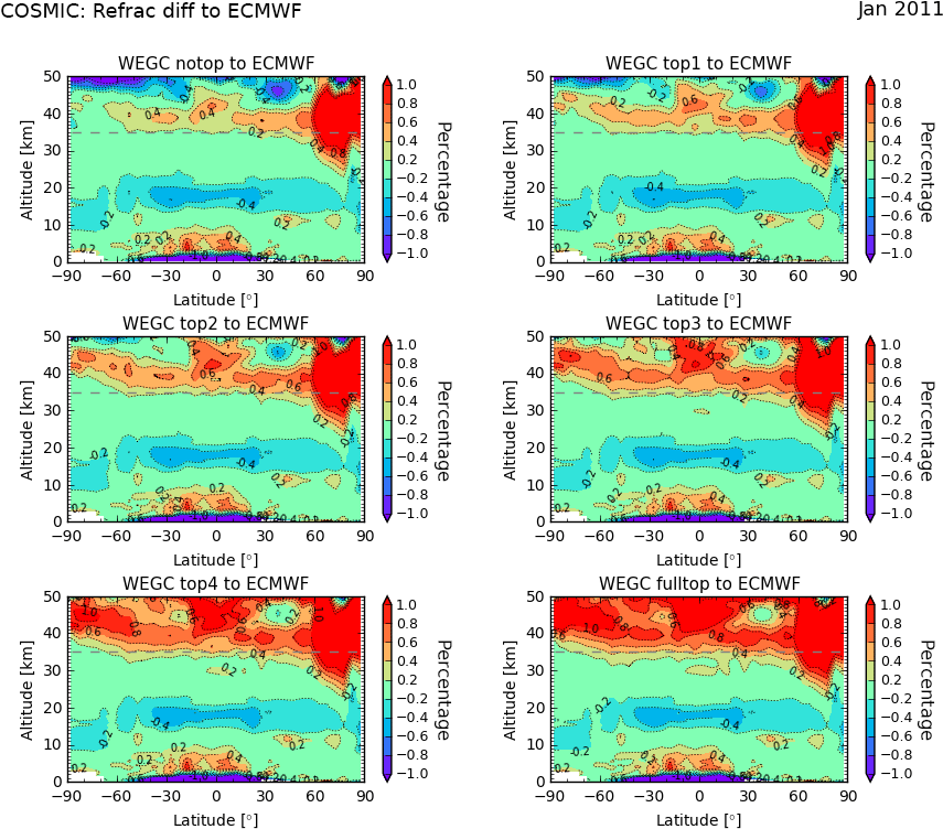
Figure 9Sensitivity of API refractivity climatologies relative to different handling of the high-altitude extrapolation, analyzed against ECMWF analyses. The plots start from a top value of zero (notop) and increase in incremental steps of 1∕5 (top1, top2, top3, top4) to the full value (fulltop).
Figure 10a shows the difference of single API refractivity climatologies compared to ECMWF analyses for six example zonal bins up to 50 km, showing the sensitivity to the extrapolation value. Clearly the notop choice usually agrees better with ECMWF, while the fulltop value shows the largest differences of around 1 % at 50 km. The sensitivity above 35 km is clear, with the largest differences between notop and fulltop of about 1 % at 50 km in altitude. Only in northern high latitudes differences are larger relative to ECMWF analyses, which could be related to different sampling of the upper stratosphere and lower mesosphere (USLM) disturbance in January 2011 (Greer et al., 2013). Related to that, the Arctic winter 2010–2011 has been noted to be one of the coldest stratospheric winters on record (Sinnhuber et al., 2011).
Figure 10b shows dry-temperature differences relative to ECMWF for the same mean API climatologies. The plot illustrates the downward propagation of the handling of the top value. The altitude differences start to increase above 20 km between the different choices of initialization, increasing to about a 2–3 K difference at 35 km in altitude relative to ECMWF analyses. Above 35 km the speed at which differences increase depends on the choice of the initialization. The choices of top3, top4, and fulltop seem to agree better relative to ECMWF analyses than notop and small initialization values, such as top1 and top2. This is not surprising, since it is clearly wrong to assume the bending angle is zero above 80 km. We also compared the different choices of top values to each other and also with the choice of exptop. It seems that the values of top3 and top4 are comparable with exptop, i.e., an exponential extrapolation.
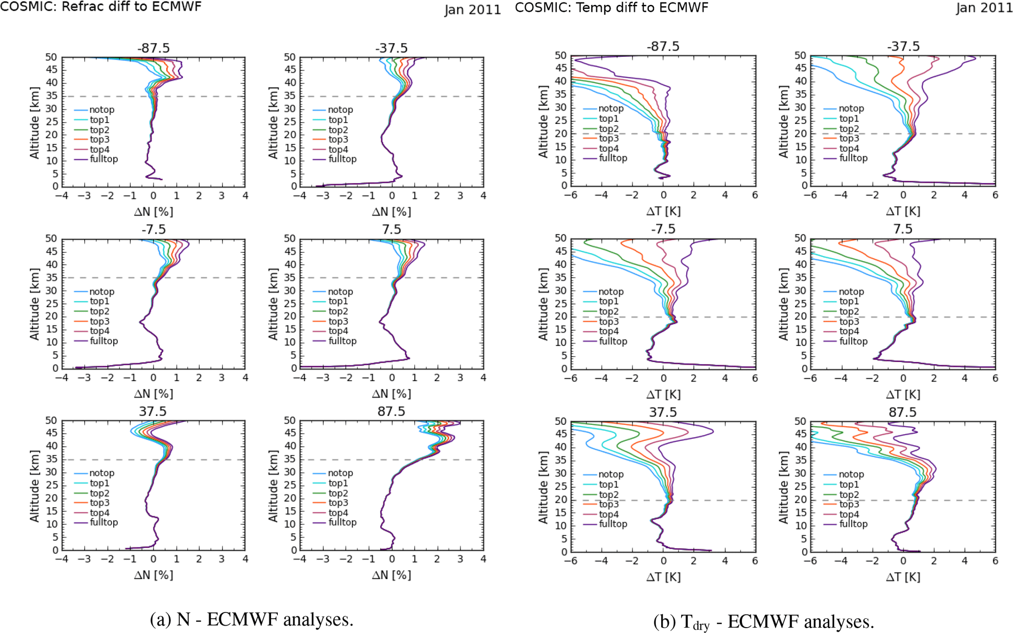
Figure 10Sensitivity of single climatological profiles relative to different handling of the altitude above 80 km, analyzed against ECMWF analyses.
5.4 API dry-temperature climatologies
In this section we analyze dry-temperature differences relative to the three reference climatologies ECMWF analyses, MIPAS, and SABER. In Fig. 11 we compare WEGC processing and DMI processing and include changes to the extrapolation. From top to bottom, we analyze WEGC fulltop, WEGC exptop, DMI exptop, and WEGC notop using the bending angle climatology DMI L1b data as input. Starting with the first column, obviously RO API climatologies are in good agreement with ECMWF analyses up to 35 km in altitude. Above 35 km, differences start to increase, depending on the choice of the high-altitude initialization. In principle notop makes no physical sense, which is why the differences are getting very large relative to ECMWF analyses. The choice exptop leads to very similar results between WEGC (second plot) and DMI (third plot) processing and agrees with ECMWF analyses up to 40 km. Temperature differences vary from 0 K to about −1 K. For the choice fulltop, differences are larger (first plot), starting at 20 km height with about 0.5 K, increasing to about 1 K at 40 km in altitude. In general, differences to ECMWF analyses tend to be larger at northern high latitudes (USLM disturbance).
Comparing the dry-temperature climatologies to MIPAS data, the general behavior seems to be relatively similar to ECMWF analyses. The WEGC and DMI exptop cases (second and third plot) agree well up to around 40 km in altitude. There are small differences in the tropics up to 35 km of −0.5 up to −1 K. The WEGC fulltop shows stronger differences around the poles compared to MIPAS than when compared to ECMWF analyses. On the other hand, SABER data (third column) also show much larger differences in the lower stratosphere, up to values of about −3 K. However, this is due to a cold bias in SABER data of about 3 K between 20 to 35 km in altitude (Innerkofler, 2015). Furthermore, SABER data show a reduced profile statistics between 90 and 55∘ S (about 400 profiles per bin, usually about 1500 profiles per latitude bin) for January 2011. The reduced statistics is clearly reflected in the SABER plots (third column, Fig. 11).
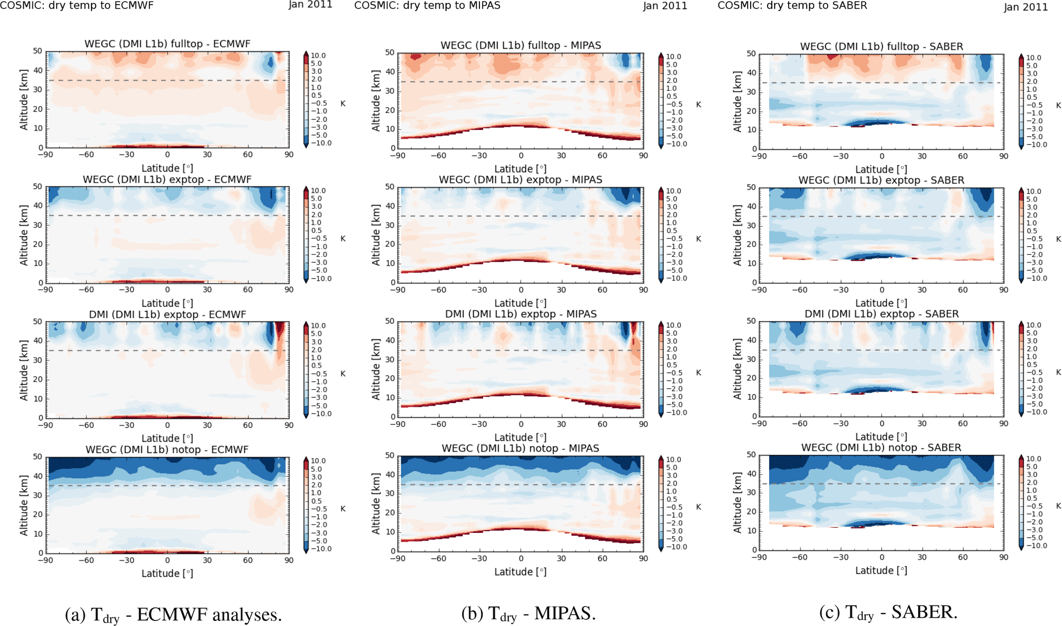
Figure 11API dry-temperature differences relative to different reference climatologies, comparing API processing between WEGC and DMI for different high-altitude extrapolations (fulltop, exptop, notop), for January 2011.
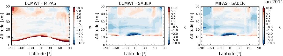
In Fig. 12 we show the differences between the three reference climatologies themselves. We want to understand up to which altitude they show good agreement between each other. Clearly, up to almost 40 km height ECMWF analyses and MIPAS (first plot) agree very well, although they still show differences of about ±0.5 K in the tropical lower stratosphere and the poles. In the polar region, temperature differences start to increase above 40 km in altitude. On the other hand, SABER clearly exhibits the cold bias in reference to ECMWF analyses (second plot) and MIPAS (third plot) between 20 and 35 km.
To summarize, since ECMWF analyses and MIPAS agree well up to altitudes of about 40 km, they appear to serve as suitable reference climatologies up to this height. Hence, we conclude from our analysis that the exponential extrapolation of WEGC exptop and DMI exptop (second and third row of Fig. 11) is a good choice for the high-altitude extrapolation of the API bending angle climatologies. Data sets between API RO climatologies (WEGC exptop and DMI exptop), ECMWF analyses, and MIPAS agree very well up to 35 km in altitude and within ±0.5 to ±1 K at 40 km.
This work is a follow-up investigation on the API retrieval method. The main idea of this method is to propagate average bending angles, instead of individual profiles through the Abel transform. The approach has already been successfully tested at DMI COSMIC data (Gleisner and Healy, 2013), as well as with CHAMP data (Danzer et al., 2014). The main focus of our work is a comparison of different implementations of the API approach at the WEGC and DMI.
We started our analysis with a first attempt at addressing the issue of calculating a single mean radius of curvature, , for a whole bin, although there can be strong variations of Rc from profile to profile. We tested different implementations of mean and found that the largest differences are in the tropical area. However, by studying the implications of the differences on the RO API dry climatologies, we find negligible impact, which supports the API approach.
Next we tested the API approach in the WEGC processing and compared it to WEGC IPI processing. Although the WEGC rOPS-ex processing system is still in development, we can conclude that differences between the two methods are very small, up to 40 km in altitude on refractivity level. Regarding dry-temperature climatologies, differences start to exceed ±1 K above 35 km. Hence we conclude that the API retrieval is a valid alternative to the standard inversion for dry-atmospheric climatologies up to about 35 km, confirming previous work at refractivity level at the DMI.
For the comparison study between WEGC and DMI we decided to use the same input bending angle climatologies from DMI using monthly 5∘ zonal COSMIC data from January to March 2011. This approach was adopted to understand differences which enter through the different processing systems and not through the input climatology. The bending angle climatologies are used up to 80 km; above that there is the need for some kind of high-altitude extrapolation due to the Abel integration to infinity. The WEGC used monthly ECMWF analysis refractivity fields to extrapolate, while DMI performed an exponential extrapolation with a fixed-scale height. While studying the resulting refractivity climatologies, we found that differences between the processing centers start to emerge at altitudes above 35 km; see Figs. 5 and 6. The observed RO–ECMWF biases above 35 km are not related to the API retrieval. They are generally seen in all RO–ECMWF comparisons when applying the standard processing (see comparison of API and IPI relative to ECMWF analyses in Figs. 5, 6, and 7 shown by Gleisner and Healy, 2013). In that context, it is interesting to see how the extrapolation above 80 km also propagates down to 35 km. This initial analysis showed that the extrapolation is a substantial issue for the API retrieval.
In a second step we decided to solely test the influence of the different implementations of the Abel integral on our resulting refractivity climatologies. To simplify the system, we switched off the high-altitude extrapolation of the average bending angles at both processing centers (notop). Furthermore, we tested an exponential extrapolation (exptop) at the WEGC and DMI. This led to good agreement between the WEGC and DMI. For notop, the mean refractivities were now almost identical up to 40 km, while for exptop they even agreed up to 50 km. It was only in the tropopause region that differences of 0.2 % remained (Figs. 7 and 8). We conclude that the different implementations of the Abel integral only play a minor role, and that the handling of the extrapolation has a much larger influence.
Next we analyzed the sensitivity of the mean climatologies to the choice of the top value. In that respect, Fig. 10 is of interest, since it shows the impact of the extrapolation on single mean refractivity climatologies as well as on the mean dry-temperature climatologies. Differences in refractivity start to increase above 35 km in altitude and for dry temperature above 20 km. Steiner et al. (2013) showed, in a comparison study of climate data products from six international processing centers, that different high-altitude initialization approaches affect uncertainties in CHAMP RO data from about 25 km upwards. The largest differences between the processing centers are found towards increasing altitudes and at high latitudes. This has also been demonstrated for the API approach in a prior study analyzing CHAMP data (Danzer et al., 2014), where differences relative to ECMWF analyses also increased towards high altitudes and latitudes. Also the API approach shows an increasing sensitivity above 35 km in altitude when comparing different high-altitude extrapolations for the bending angle and comparing WEGC and DMI processing centers. The propagation of errors downwards through the API retrieval chain to about 20 km in dry temperature shown here has also been observed in prior studies for standard retrievals from different processing centers (Foelsche et al., 2011; Ho et al., 2012; Steiner et al., 2013).
Finally, we investigated dry-temperature climatologies with respect to ECMWF analyses, MIPAS, and SABER. We also compared different choices of the high-altitude extrapolation (fulltop, exptop, notop) in the WEGC and DMI processing (see Fig. 11). In general RO API data sets agree well with the reference data sets up to 35 km in altitude. In the case of an exponential extrapolation (exptop) they even have good agreement up to 40 km in altitude for both the processing system at WEGC and at DMI. Only the fulltop leads to enhanced differences starting at about 20 km in altitude with 0.5 K, increasing to about 1 K at 40 km in altitude. The temperature comparison study of RO API data sets relative to ECMWF analyses, MIPAS, and SABER data sets shows similar temperature biases for both the WEGC and the DMI exptop case, as Innerkofler (2015) found by analyzing global RO IPI temperature data sets. RO API, ECMWF analysis data, and MIPAS data agree within ±1 K, up to 40 km. Above 40 km they begin to show larger differences than when analyzing global RO IPI data. Furthermore, the 3 K temperature bias of SABER data could also clearly be illustrated relative to RO API data.
In further work we plan to investigate the issue of ionospheric residuals in the bending angle data. For that, we will apply the higher-order ionospheric correction method (Angling et al., 2018; Danzer et al., 2015; Healy and Culverwell, 2015). This correction method is based on the difference of the L1/L2 bending angles squared and a scaling term κ, which depends on solar zenith angle, solar flux, and altitude. It will be interesting to see whether residual ionospheric noise in the data is reduced and the data quality of the climatologies can be raised to higher altitudes.
In summary we conclude that the API retrieval is a valid alternative and, with respect to computation time, even much faster for the production of dry-atmospheric RO climatologies. It shows a robustness between the processing centers WEGC and DMI up to about 35 km in altitude if different high-altitude extrapolations are used. Applying an exponential extrapolation at both centers produces dry-temperature climatologies that agree with each other, ECMWF analyses, and MIPAS climatologies up to 40 km in altitude within ±1 K. The latter result might suggests that API dry-temperature climatologies can be used up to 40 km, pushing current limits of the utility of RO data into the stratosphere.
The rOPS-ex and ROPP RO data sets are available from the corresponding author upon reasonable request.
JD performed the computational implementation and the analysis, created the figures, and wrote the paper, except for the introduction. MS provided computational advice and support. VP computed the rOPS-ex bending angle data. UF wrote the introduction, provided general guidance, and looked over a previous version of the paper. HG computed all DMI climatologies and also looked over a previous version of the paper.
The authors declare that they have no conflict of interest.
We thank UCAR/CDAAC for providing COSMIC excess phase data, and the ECMWF for
providing analysis data. Furthermore, we thank Gottfried Kirchengast for his support
and for discussions, and Sean Healy for final proofreading. Our work was funded
by the Austrian Science Fund (FWF) as a Hertha Firnberg-Project under grant T
757-N29 (NEWCLIM project). Hans Gleisner was supported by the ROM SAF, which is
a decentralized operational RO processing center under EUMETSAT. We thank the
ROM SAF for providing reprocessed GPS-RO data.
Edited by: Lars Hoffmann
Reviewed by: two anonymous referees
Angling, M. J., Elvidge, S., and Healy, S. B.: Improved model for correcting the ionospheric impact on bending angle in radio occultation measurements, Atmos. Meas. Tech., 11, 2213–2224, https://doi.org/10.5194/amt-11-2213-2018, 2018. a
Anthes, R. A.: Exploring Earth's atmosphere with radio occultation: contributions to weather, climate and space weather, Atmos. Meas. Tech., 4, 1077–1103, https://doi.org/10.5194/amt-4-1077-2011, 2011. a
Ao, C. O., Mannucci, A. J., and Kursinski, E. R.: Improving GPS Radio Occultation Stratospheric Refractivity Retrievals for Climate Benchmarking, Geophys. Res. Lett., 39, 12, https://doi.org/10.1029/2012GL051720, 2012. a
Cardinali, C.: Monitoring the observation impact on the short-range forecast, Q. J. Roy. Meteor. Soc., 135, 239–250, 2009. a
Culverwell, I. D., Lewis, H. W., Offiler, D., Marquardt, C., and Burrows, C. P.: The Radio Occultation Processing Package, ROPP, Atmos. Meas. Tech., 8, 1887–1899, https://doi.org/10.5194/amt-8-1887-2015, 2015. a
Danzer, J., Gleisner, H., and Healy, S. B.: CHAMP climate data based on the inversion of monthly average bending angles, Atmos. Meas. Tech., 7, 4071–4079, https://doi.org/10.5194/amt-7-4071-2014, 2014. a, b, c, d, e, f, g
Danzer, J., Healy, S. B., and Culverwell, I. D.: A simulation study with a new residual ionospheric error model for GPS radio occultation climatologies, Atmos. Meas. Tech., 8, 3395–3404, https://doi.org/10.5194/amt-8-3395-2015, 2015. a
Foelsche, U., Borsche, M., Steiner, A. K., Gobiet, A., Pirscher, B., Kirchengast, G., Wickert, J., and Schmidt, T.: Observing upper troposphere-lower stratosphere climate with radio occultation data from the CHAMP satellite, Clim. Dynam., 31, 49–65, https://doi.org/10.1007/s00382-007-0337-7, 2008a. a
Foelsche, U., Kirchengast, G., Steiner, A. K., Kornblueh, L., Manzini, E., and Bengtsson, L.: An observing system simulation experiment for climate monitoring with GNSS radio occultation data: Setup and test bed study, J. Geophys. Res., 113, D11108, https://doi.org/10.1029/2007JD009231, 2008b. a, b
Foelsche, U., Pirscher, B., Borsche, M., Kirchengast, G., and Wickert, J.: Assessing the climate monitoring utility of radio occultation data: From CHAMP to FORMOSAT-3/COSMIC, Terr. Atmos. Ocean. Sci., 20, 155–170, https://doi.org/10.3319/TAO.2008.01.14.01(F3C), 2009. a
Foelsche, U., Scherllin-Pirscher, B., Ladstädter, F., Steiner, A. K., and Kirchengast, G.: Refractivity and temperature climate records from multiple radio occultation satellites consistent within 0.05 %, Atmos. Meas. Tech., 4, 2007–2018, https://doi.org/10.5194/amt-4-2007-2011, 2011. a, b
García-Comas, M., Funke, B., López-Puertas, M., Bermejo-Pantaleón, D., Glatthor, N., von Clarmann, T., Stiller, G., Grabowski, U., Boone, C. D., French, W. J. R., Leblanc, T., López-González, M. J., and Schwartz, M. J.: On the quality of MIPAS kinetic temperature in the middle atmosphere, Atmos. Chem. Phys., 12, 6009–6039, https://doi.org/10.5194/acp-12-6009-2012, 2012. a
Gleisner, H. and Healy, S. B.: A simplified approach for generating GNSS radio occultation refractivity climatologies, Atmos. Meas. Tech., 6, 121–129, https://doi.org/10.5194/amt-6-121-2013, 2013. a, b, c, d, e, f, g, h, i, j, k, l
Gobiet, A. and Kirchengast, G.: Advancements of Global Navigation Satellite System radio occultation retrieval in the upper stratosphere for optimal climate monitoring utility, J. Geophys. Res., 109, D24110, https://doi.org/10.1029/2004JD005117, 2004. a
Gorbunov, M. E.: Canonical transform method for processing radio occultation data in the lower troposphere, Radio Sci., 37, 5, https://doi.org/10.1029/2000RS002592, 2002. a
Gorbunov, M. E. and Kirchengast, G.: Wave-optics uncertainty propagation and regression-based bias model in GNSS radio occultation bending angle retrievals, Atmos. Meas. Tech., 11, 111–125, https://doi.org/10.5194/amt-11-111-2018, 2018. a
Gorbunov, M. E. and Lauritsen, K. B.: Analysis of wave fields by Fourier integral operators and their application for radio occultations, Radio Sci., 39, RS4010, https://doi.org/10.1029/2003RS002971, 2004. a
Greer, K., Thayer, J., and Harvey, V.: A climatology of polar winter stratopause warmings and associated planetary wave breaking, J. Geophys. Res.-Atmos., 118, 4168–4180, 2013. a
Healy, S. B. and Culverwell, I. D.: A modification to the standard ionospheric correction method used in GPS radio occultation, Atmos. Meas. Tech., 8, 3385–3393, https://doi.org/10.5194/amt-8-3385-2015, 2015. a
Healy, S. B. and Thépaut, J. N.: Assimilation experiments with CHAMP GPS radio occultation measurements, Q. J. Roy. Meteor. Soc., 132, 605–623, https://doi.org/10.1256/qj.04.182, 2006. a
Ho, S.-P., Kirchengast, G., Leroy, S., Wickert, J., Mannucci, A. J., Steiner, A. K., Hunt, D., Schreiner, W., Sokolovskiy, S., Ao, C., Borsche, M., von Engeln, A., Foelsche, U., Heise, S., Iijima, B., Kuo, Y.-H., Kursinski, E. R., Pirscher, B., Ringer, M., Rocken, C., and Schmidt, T.: Estimating the uncertainty of using GPS radio occultation data for climate monitoring: Intercomparison of CHAMP refractivity climate records from 2002 to 2006 from different data centers, J. Geophys. Res., 114, D23107, https://doi.org/10.1029/2009JD011969, 2009. a
Ho, S.-P., , Hunt, D., Steiner, A. K., Mannucci, A. J., Kirchengast, G., Gleisner, H., Heise, S., von Engeln, A., Marquardt, C., Sokolovskiy, S., Schreiner, W., Scherllin-Pirscher, B., Ao, C., Wickert, J., Syndergaard, S., Lauritsen, K. B., Leroy, S., Kursinski, E. R., Kuo, Y.-H., Foelsche, U., Schmidt, T., and Gorbunov, M.: Reproducibility of GPS radio occultation data for climate monitoring: Profile-to-profile inter-comparison of CHAMP climate records 2002 to 2008 from six data centers, J. Geophys. Res., 117, D18111, https://doi.org/10.1029/2012JD017665, 2012. a, b, c, d
Innerkofler, J.: Evaluation of the climate utility of radio occultation data in the upper stratosphere and mesosphere (MSc thesis), Sci. Rep. 65-2015, 154 pp., Wegener Center Verlag, Graz, Austria, 2015. a, b, c
Kirchengast, G., Schwärz, M., Scherllin-Pirscher, B., Pock, C., Innerkofler, J., Proschek, V., Steiner, A., Danzer, J., Ladstädter, F., and Foelsche, U.: The reference occultation processing system approach to interpret GNSS radio occultation as SI-traceable planetary system refractometer, OPAC-IROWG 2016 International Workshop, 8–14 September, Seggau Castle, Austria, 2016. a
Kirchengast, G., Schwärz, M., Schwarz, J., Ramsauer, J., Fritzer, J., Scherllin-Pirscher, B., Innerkofler, J., Proschek, V., Rieckh, T., and Danzer, J.: Reference OPS DAD – Reference Occultation Processing System (rOPS) Detailed Algorithm Description, Tech. Rep. for ESA and FFG No. 1/2017, Doc-Id: WEGC–rOPS–2017–TR01, Issue 1.7, Wegener Center, University of Graz, 2017. a, b
Kursinski, E. R., Hajj, G. A., Schofield, J. T., Linfield, R. P., and Hardy, K. R.: Observing Earth's atmosphere with radio occultation measurements using the Global Positioning System, J. Geophys. Res., 102, 23429–23465, 1997. a
Lauritsen, K. B., Syndergaard, S., Gleisner, H., Gorbunov, M. E., Rubek, F., Sørensen, M. B., and Wilhelmsen, H.: Processing and validation of refractivity from GRAS radio occultation data, Atmos. Meas. Tech., 4, 2065–2071, https://doi.org/10.5194/amt-4-2065-2011, 2011. a
Leroy, S. S., Anderson, J. G., and Dykema, J. A.: Testing climate models using GPS radio occultation: A sensitivity analysis, J. Geophys. Res., 11, D17105, https://doi.org/10.1029/2005JD006145, 2006. a
Li, Y., Kirchengast, G., Scherllin-Pirscher, B., Wu, S., Schwaerz, M., Fritzer, J., Zhang, S., Carter, B. A., and Zhang, K.: A new dynamic approach for statistical optimization of GNSS radio occultation bending angles for optimal climate monitoring utility, J. Geophys. Res.-Atmos., 118, 13022–13040, https://doi.org/10.1002/2013JD020763, 2013. a
Li, Y., Kirchengast, G., Scherllin-Pirscher, B., Norman, R., Yuan, Y. B., Fritzer, J., Schwaerz, M., and Zhang, K.: Dynamic statistical optimization of GNSS radio occultation bending angles: advanced algorithm and performance analysis, Atmos. Meas. Tech., 8, 3447–3465, https://doi.org/10.5194/amt-8-3447-2015, 2015. a
Lohmann, M. S.: Application of dynamical error estimation for statistical optimization of radio occultation bending angles, Radio Sci., 40, 2005. a
Ringer, M. A. and Healy, S. B.: Monitoring twenty-first century climate using GPS radio occultation bending angles, Geophys. Res. Lett., 35, L05708, https://doi.org/10.1029/2007GL032462, 2008. a
Scherllin-Pirscher, B.: Further development of BAROCLIM and implementation in ROPP, Tech. rep., GRAS-SAF, cDOP-2 Visiting Scientist Report 19. Ref: SAF/GRAS/DMI/REP/VS19/001, 56 pp., 2013. a
Scherllin-Pirscher, B., Syndergaard, S., Foelsche, U., and Lauritsen, K. B.: Generation of a bending angle radio occultation climatology (BAROCLIM) and its use in radio occultation retrievals, Atmos. Meas. Tech., 8, 109–124, https://doi.org/10.5194/amt-8-109-2015, 2015. a, b
Schwarz, J., Kirchengast, G., and Schwaerz, M.: Integrating uncertainty propagation in GNSS radio occultation retrieval: from excess phase to atmospheric bending angle profiles, Atmos. Meas. Tech., 11, 2601–2631, https://doi.org/10.5194/amt-11-2601-2018, 2018. a
Schwarz, J. C., Kirchengast, G., and Schwaerz, M.: Integrating uncertainty propagation in GNSS radio occultation retrieval: from bending angle to dry-air atmospheric profiles, Earth Space Sci., 4, 200–228, https://doi.org/10.1002/2016EA000234, 2017. a
Sinnhuber, B.-M., Stiller, G., Ruhnke, R., Clarmann, T., Kellmann, S., and Aschmann, J.: Arctic winter 2010/2011 at the brink of an ozone hole, Geophys. Res. Lett., 38, 24, 2011. a
Sokolovskiy, S. V., Schreiner, W. S., Rocken, C., and Hunt, D.: Optimal noise filtering for the ionospheric correction of GPS radio occultation signals, J. Atmos. Ocean. Tech., 26, 1398–1403, https://doi.org/10.1175/2009JTECHA1192.1, 2009. a
Steiner, A. K., Kirchengast, G., Foelsche, U., Kornblueh, L., Manzini, E., and Bengtsson, L.: GNSS occultation sounding for climate monitoring, Phys. Chem. Earth A, 26, D09102, https://doi.org/10.1016/S1464-1895(01)00034-5, 2001. a
Steiner, A. K., Hunt, D., Ho, S.-P., Kirchengast, G., Mannucci, A. J., Scherllin-Pirscher, B., Gleisner, H., von Engeln, A., Schmidt, T., Ao, C., Leroy, S. S., Kursinski, E. R., Foelsche, U., Gorbunov, M., Heise, S., Kuo, Y.-H., Lauritsen, K. B., Marquardt, C., Rocken, C., Schreiner, W., Sokolovskiy, S., Syndergaard, S., and Wickert, J.: Quantification of structural uncertainty in climate data records from GPS radio occultation, Atmos. Chem. Phys., 13, 1469–1484, https://doi.org/10.5194/acp-13-1469-2013, 2013. a, b, c, d
Syndergaard, S. and Kirchengast, G.: An Abel transform for deriving line-of-sight wind profiles from LEO-LEO infrared laser occultation measurements, J. Geophys. Res., 121, 2525–2541, https://doi.org/10.1002/2015JD023535, 2016. a
Torge, W.: Geodesy, Third completely revised and extended edition, Walter de Gruyter, Berlin, New York, 2001. a