the Creative Commons Attribution 4.0 License.
the Creative Commons Attribution 4.0 License.
 | 15 Feb 2018
Assessment of surface solar irradiance derived from real-time modelling techniques and verification with ground-based measurements
Panagiotis G. Kosmopoulos
Stelios Kazadzis
Michael Taylor
Panagiotis I. Raptis
Iphigenia Keramitsoglou
Chris Kiranoudis
Alkiviadis F. Bais
This study focuses on the assessment of surface solar radiation (SSR) based on operational neural network (NN) and multi-regression function (MRF) modelling techniques that produce instantaneous (in less than 1 min) outputs. Using real-time cloud and aerosol optical properties inputs from the Spinning Enhanced Visible and Infrared Imager (SEVIRI) on board the Meteosat Second Generation (MSG) satellite and the Copernicus Atmosphere Monitoring Service (CAMS), respectively, these models are capable of calculating SSR in high resolution (1 nm, 0.05∘, 15 min) that can be used for spectrally integrated irradiance maps, databases and various applications related to energy exploitation. The real-time models are validated against ground-based measurements of the Baseline Surface Radiation Network (BSRN) in a temporal range varying from 15 min to monthly means, while a sensitivity analysis of the cloud and aerosol effects on SSR is performed to ensure reliability under different sky and climatological conditions. The simulated outputs, compared to their common training dataset created by the radiative transfer model (RTM) libRadtran, showed median error values in the range −15 to 15 % for the NN that produces spectral irradiances (NNS), 5–6 % underestimation for the integrated NN and close to zero errors for the MRF technique. The verification against BSRN revealed that the real-time calculation uncertainty ranges from −100 to 40 and −20 to 20 W m−2, for the 15 min and monthly mean global horizontal irradiance (GHI) averages, respectively, while the accuracy of the input parameters, in terms of aerosol and cloud optical thickness (AOD and COT), and their impact on GHI, was of the order of 10 % as compared to the ground-based measurements. The proposed system aims to be utilized through studies and real-time applications which are related to solar energy production planning and use.
- Article
(7935 KB) - Full-text XML
- BibTeX
- EndNote


Solar energy exploitation is a cornerstone for sustainable development, through efficient energy planning, towards the goal of gradual independence from fossil fuels. In this direction, the European Union (EU), the Middle East and North Africa (MENA) and numerous neighbouring regions and countries have laid out specific technology roadmaps aiming at the integration of low carbon energy technologies linked with the deployment of photovoltaic (PV) installations in the energy market (IPCC, 2012; NREL, 2016; IRENA, 2016; Jager-Waldau, 2016; REN21, 2017; UN, 2017). In addition, the United Nations (2017) has set as its main sustainable development goal by 2030 to ensure universal access to affordable, reliable, and modern energy services. The International Energy Agency (2007) has estimated that the global primary energy demand will increase by 40–50 % from 2003 to 2030. Since energy production, transportation and consumption put considerable pressure on the environment, there is serious concern regarding the sustainability of energy consumption.
Earth observation (EO)-based systems and relevant services already play an important role in the solar energy industry, as well as in human-health-related emerging technologies, but there is still significant potential in increasing their efficiency and exploitation (Schroedter-Homscheidt et al., 2006; Wald et al., 2011; Lefevre et al., 2014). EO from space is already triggering services and applications that can deliver benefits throughout all the phases of energy production and supply. Their contribution ranges from identifying reservoirs and locations with solar energy potential to controlling and monitoring of the distribution networks across Europe, Africa and the Middle East, while providing support to energy policy formulation and enforcement (EU, 2011; IEA, 2010).
The need for improved EO-based surface solar irradiance assessment is increasing as more solar farms are included in national electricity grids worldwide (EC, 2013). Solar-energy-related installations have been increasing their share on the total energy demand as defined by the distribution and transmission system operators (DSOs and TSOs, respectively). As a result, accurate, real-time and short-term forecasting estimations of surface solar radiation (SSR) and, more specifically, global horizontal irradiance (GHI) related to the operation principles of PV installations are vital. The real-time GHI estimations are required at local and regional scales, as well as high temporal frequency (every 5–15 min), in order to be used for near-real-time decisions, linked with the PV-related contribution to the electricity grid.
Since the launch of EO satellites, such as Meteosat Second Generation (MSG), and Sentinel satellite series, real-time image processing techniques have been developed (Suárez and Nesmachnow, 2012). The main advantage of these techniques is the possibility to monitor numerous meteorological variables in almost real time (Derrien et al., 2005; MeteoFrance, 2013). A comprehensive intercomparison of radiation products, codes, algorithms, models and independent databases has been performed by many researchers (Oreopoulos and Mlawer, 2010; Oreopoulos et al., 2012; Ellingson et al., 1991; Ineichen, 2006; Beyer et al., 2009; Cahalan, et al., 2005). Solid steps in estimating the surface GHI were taken by Deneke and Feijt (2008), Schulz et al. (2009), Mueller et al. (2009), Huang et al. (2011) and Qu et al. (2017), who developed GHI retrieval methodologies based on the use of discrete pre-calculated look-up tables (LUTs), while Dorvlo et al. (2002), Zarzalejo et al. (2005), Lopez et al. (2001) and Takenaka et al. (2011) developed solutions based on neural network (NN) models. The validation of most of the above mentioned methodologies was performed against radiative transfer model (RTM) simulations and ground-based measurements, from various networks around the globe. However, from the validation results it was shown that accuracy was inversely proportional to calculation speed under all-sky and terrain conditions. The magnitude of the GHI uncertainty due to the effect of aerosols and clouds is significant and has motivated numerous related studies (Federico et al., 2017; Kosmopoulos et al., 2015; Lara-Fanego et al., 2012; Tegen et al., 1996; Lindfors et al., 2013). Under high aerosol loads the SSR can be reduced by 20–50 % (Eck et al., 1998; Gleeson et al., 2016; Kosmopoulos et al., 2017), while under cloudy conditions the impact was up to 60–90 % for overcast conditions and cloud coverage of 8 octas (Aebi, et al., 2017; Kosmopoulos et al., 2015; Zygmuntowska et al., 2012), highlighting the significant effect of these atmospheric parameters (clouds and aerosols) on the GHI calculations and in the performance of PV installations and energy production.
In the present study, we report on (i) the assessment of the surface solar irradiance calculated in real time, which is defined as the product with a time delay of 1 min or less from an actual atmospheric situation, by developing and using two NN-based techniques and a multi-regression-function-based technique and (ii) the validation of these techniques against ground-based measurements from the Baseline Surface Radiation Network (BSRN). Section 2 presents data, methods and techniques used. Section 3 describes the validation results including a sensitivity analysis of related atmospheric parameters and in Sect. 4 we present our conclusions on the proposed techniques.
Table 1Coordinates (degrees) and height (metres above sea level) of the BSRN stations used for the validation.
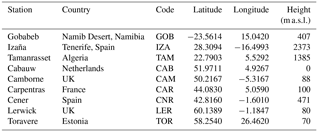
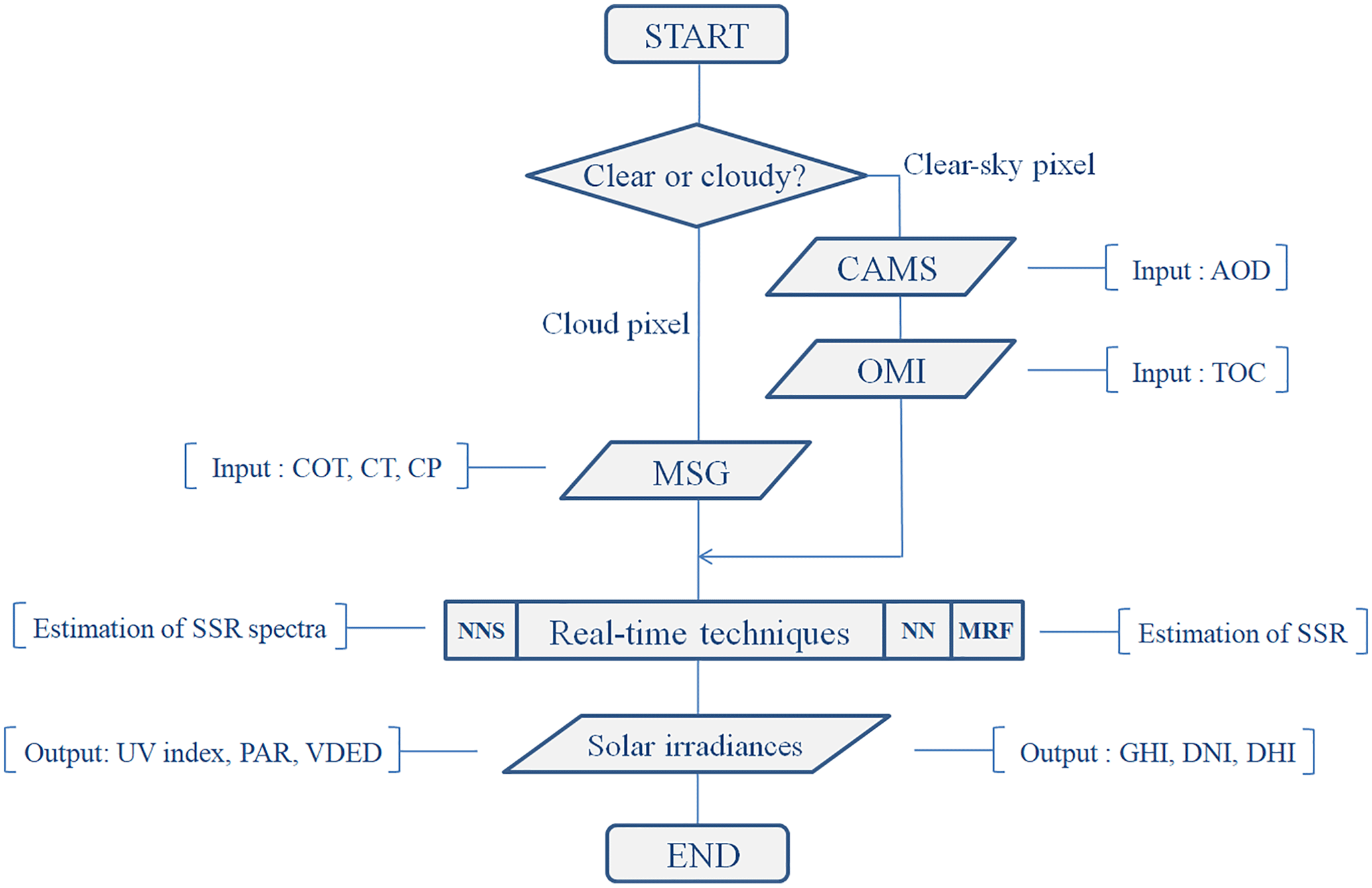
Figure 1Flowchart of the modelling technique scheme. The initial pixel classification followed by the clear- or cloudy-sky inputs to the real-time solver result the spectral (NNS) and integrated (MRF and NN) SSR-related outputs.
2.1 Data
2.1.1 Ground-based measurements
The verification of the applied SSR real-time modelling techniques was performed against ground-based measurements from nine stations (Table 1) of the Baseline Surface Radiation Network (BSRN; Hegner et al., 1998) equipped with Kipp and Zonen pyranometers (GHI measurements) and a precision filter radiometer (PFR) at Izaña, Spain. BSRN consists of high-quality ground-based measurements of SSR and for the purposes of the comparison we used the dataset from July 2014 to June 2015. Table 1 presents the location and description of the nine BSRN stations used for the validation of the SSR estimations calculated with the modelling techniques. The temporal resolution of the ground-based measurements is 1 min, so in order to match the 15 min resolution of the MSG cloud data (and hence the SSR outputs) we used 15 min averages of all the BSRN and PFR measurements used. The selected BSRN stations represent a variety of different climates, altitudes and aerosol sources in the field of view of MSG and thus provide an opportunity to study the models' performance under various atmospheric conditions.
2.1.2 Real-time cloud observations
The most important inputs to our real-time modelling techniques were the satellite cloud data products from the Spinning Enhanced Visible and Infrared Imager (SEVIRI) on board the Meteosat Second Generation (MSG) satellite. We obtained the cloud type (CT), the cloud phase (CP) and the cloud optical thickness (COT) products so as to efficiently quantify the effect of clouds on SSR. COT depends on the moisture density as well as the vertical thickness of the cloud. The cloud reflectance at channel at 0.6 µm in the visible part of the electromagnetic spectrum is directly related to COT (Roebeling et al., 2006). The MSG geostationary satellite, because of its orbit height (36 000 km above the Equator), allows the continuous monitoring over Europe, Africa and parts of South America at high temporal and spatial resolution (15 min and 0.05∘, respectively). The operational MSG-SEVIRI data were acquired by the EUMETCast station operated by the Institute for Astronomy, Astrophysics, Space Applications and Remote Sensing of the National Observatory of Athens. The cloud properties are extracted operationally and in real time using the Satellite Application Facility for Nowcasting Weather Conditions software (SAFNWC) installed in-house. CT and CP are standard output products of the SAFNWC computational procedure, while COT is a tailor-made product and as a result its extraction required an additional intervention in the process chain. The cloud product identification is described in Derrien and Gléau (2005) and the MétéoFrance (2013) technical report. In the current implementation, cloud products are provided operationally for the entire Earth disc view area of MSG. We extracted products at specific pixels corresponding to locations of the BSRN stations, which were used as inputs to the SSR modelling techniques.
2.1.3 Aerosol forecasts
For the real-time assessment of the SSR we additionally incorporated the aerosol 1-day forecast data from the Copernicus Atmospheric Monitoring Service (CAMS) as the basic input parameter. These forecasts are based on the Monitoring Atmospheric Composition and Climate (MACC) reanalysis tools, and include validated modelling of aerosol and satellite data assimilation (Eskes et al., 2015). They are able to provide operationally accurate data of aerosol optical depth (AOD) at 550 nm, at 1 h time steps and 0.4∘ spatial resolution. The estimation of the aerosol sources is extracted from the Emission Database for Global Atmospheric Research (EDGAR) and the Speciated Particulate Emission Wizard (SPEW), while the reliability of the product is supported by continuous assimilation into the model of the MODIS AOD data, applying a bias correction from multiple data sources (Dee and Uppala, 2009). For the purposes of our SSR estimations, the CAMS AOD forecasts with the MSG COT data described above constitute the most important input parameters, together with solar elevation, for the SSR retrieval modelling tools.
2.2 Methodology
In this section we present the SSR real-time modelling techniques, the methodology used for developing operational products and the validation statistics against ground-based measurements. The techniques are the multi-regression function (MRF), the neural network that produces spectral irradiances (NNS) and which is presented in detail in Taylor et al. (2015), and a variant version of the NN that produces integrated irradiances. All three techniques have been optimized based on LUTs that are described in the Sect. 2.2.1 and produce instantaneous (with less than 1 min delay from the time that the MSG image is produced) SSR. The number of outputs depends on the region under study and can be of the order of 106 simulations simultaneously. In this study we used the CAMS AOD and the MSG COT as operational inputs, in conjunction with the solar elevation angle, as they are the major attenuators of the GHI. Since the comparison of real-time modelling techniques with ground-based measurements are performed from southern Africa to northern Europe, the verification will be focused on GHI. Utilization of the direct normal irradiance (DNI) by concentrated solar power (CSP) plants is limited at places with high amounts of DNI (Green et al., 2015), and hence CSPs are de facto outside of energy planning for the majority of the countries represented by the nine BSRN stations and the MSG view. Large-scale, high temporal and spatial resolution EO-based assessment of the SSR seems to be an emerging market prospect (ITA, 2016). The potential application fields of the methodology proposed in this study include the production planning support on large-scale solar farm projects and the efficient control of the electricity balancing and distribution (in support of the TSOs and DSOs) by incorporating the produced energy of the solar farms into the electricity grid. At the same time, SSR in different spectral regions highlight spectrally weighted outputs like the UV index (linked with skin cancer, eye cataracts, DNA damage etc.), vitamin D efficiency (related to pregnancy) and a number of agricultural and oceanographical related processes (plant photosynthesis, crop production, phytoplankton growth etc.). As a result, the developed real-time modelling techniques are able to assist public authorities in energy-planning policies; support the work of various scientific communities dealing with health protection, energy production and consumption and solar energy exploitation; and finally enable the solar industry to better plan clean energies, its transmission and distribution, which in turn will boost the relative contribution to national portfolios. Figure 1 illustrates the procedural flows of the three developed real-time modelling techniques for operational use. Starting with the MSG cloud flags (0 = clear sky and 1, 2, 3 = cloudy sky in terms of water, ice and mixed clouds, respectively), we identify the clear-sky and cloudy-sky pixels. For the cloudy pixels we incorporate the optical properties (COT) and types of clouds (CT), while for clear-sky pixels we take into account the aerosol effect (AOD) and the total ozone column (TOC), which was derived using Ozone Monitoring Instrument (OMI) retrievals (Wandji-Nyamsi et al., 2015). Then, for all-sky conditions we generate the input files to the real-time techniques and, depending on their special characteristics, we produce spectral or spectrally weighted products (see following subsections) at high spectral, spatial and temporal resolution (1 nm, 0.05∘, 15 min). The actual outputs can be SSR time series, local and regional maps or Earth disc view maps (Fig. 2).
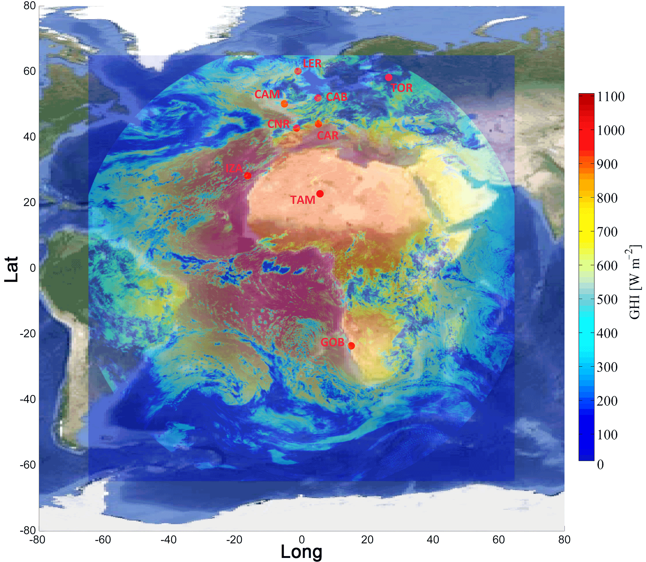
Figure 2An example of the output maps based on the real-time SSR techniques. Here is the GHI for 15 April 2015 at 12:00 UTC together with the BSRN station locations.
The performance of the real-time techniques was evaluated by comparing the GHI outputs with (i) the initial RTM simulation LUTs and (ii) the BSRN ground-based measurements and with respect to the aerosol and cloud effects. The evaluation was based on the bias and mean bias error (MBE), the root mean square error (RMSE) and their relative components (rMBE and rRMSE, respectively):
The residuals (estimation errors), , are calculated as the difference between the estimated values by the real-time techniques (xe) and the measured values (x0) by BSRN, where N is the total number of data. MBE measures the overall bias and detects the model's overestimation (MBE > 0) or underestimation (MBE < 0). RMSE quantifies the spread in the distribution of errors. Concerning the rMBE and rRMSE error measures, the normalization is done with respect to the mean ground measurement irradiance in the considered station and period. In addition, for the various tests performed in this study we calculated the slope, the correlation coefficient (r), the coefficient of determination (r2), the percentage difference (%), the mean absolute difference and the standard deviation.
Table 2RTM-simulated GHI at 15 min time intervals as compared to the BSRN ground-based measurements in terms of correlation coefficient (r) and slope.
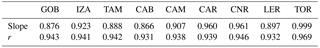
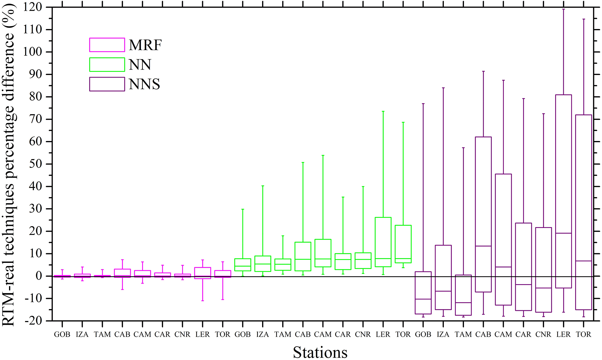
Figure 3Percentage difference (%) of the real-time modelling techniques as compared to the RTM simulations for all ground stations. The box charts highlight the more precise estimation approach of the MRF technique as compared to the NN-based techniques.
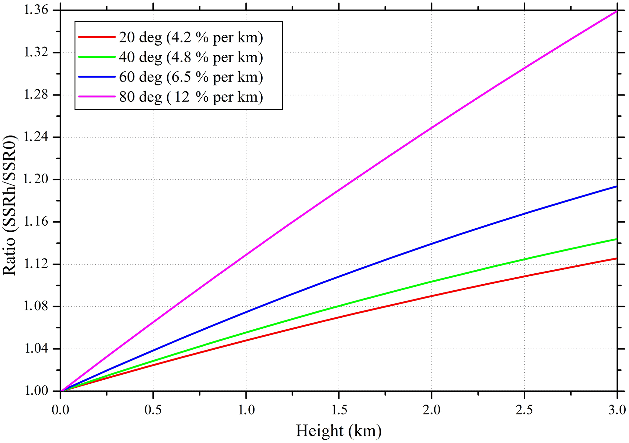
Figure 4The altitude correction of GHI for various SZAs as a function of the SSR ratio (SSR at height h compared to SSR at sea level).
2.2.1 Radiative transfer model
All modelling techniques presented in this paper for the real-time assessment of the SSR are based on LUTs, calculated with the radiative transfer model (RTM) libRadtran (Mayer and Kylling, 2005; Emde et al., 2016). These LUTs are described in detail in Taylor et al. (2015) and consist of more than 2.5 million RTM simulations with atmospheric inputs and 1 nm spectral resolution GHI outputs. The interoperable exchange of similar GHI databases is studied by Ménard et al. (2015), highlighting the usefulness and necessity of such LUT-based approaches (Lefevre et al., 2014). Under clear-sky conditions the simulated by libRadtran input parameters were the solar zenith angle (SZA), the AOD, the Ångström exponent (AE), the single-scattering albedo (SSA), TOC and the columnar water vapour (WV), while under cloudy conditions except from SZA and TOC, we also used the optical thicknesses of water and ice clouds (WCOT and ICOT, respectively) as inputs. The AOD is not used for cloudy conditions when COT > 1, as the effects of aerosols are much weaker compared to thick clouds. For the model versus BSRN station comparison, in order to take into account the station altitude, an altitude correction on the solar energy output of the different model simulations has been applied based on RTM (Libradtran) calculations. The outputs are high-resolution spectral irradiances (1 nm) covering the wavelength region between 285 and 2700 nm. In brief, we used the SDISORT radiative transfer solver (Dahlback and Stamnes, 1991) with pseudospherical approximation to produce valid outputs from 0 to 90∘ SZA; the simulations were calculated using a band parameterization method based on the correlated-K approximation (Kato et al., 1999), while the aerosol and cloud determination was performed based on the default aerosol model described by Shettle (1989) and typical cases for the height of water and ice clouds, the effective radius (Reff) and the liquid water path (Hess et al., 1998). All the technical and structural information about the RTM simulations, the input parameters and the construction of the LUTs is presented in Taylor et al. (2015). Table 2 presents the slope and the correlation coefficient between the RTM simulations of GHI and the BSRN ground-based measurements for the whole datasets and period. The overall accuracy in terms of slope ranges from 0.866 (CAB) to almost 1 (0.999 at TOR), while the r values range between 0.93 and 0.97.
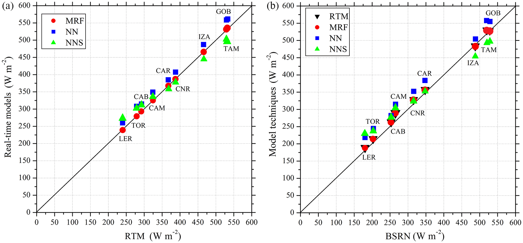
Figure 5The mean GHI in W m−2 of the real-time modelling techniques as compared to the RTM simulations for all ground stations (a), and the mean GHI of all models as compared to the BSRN measurements (b).
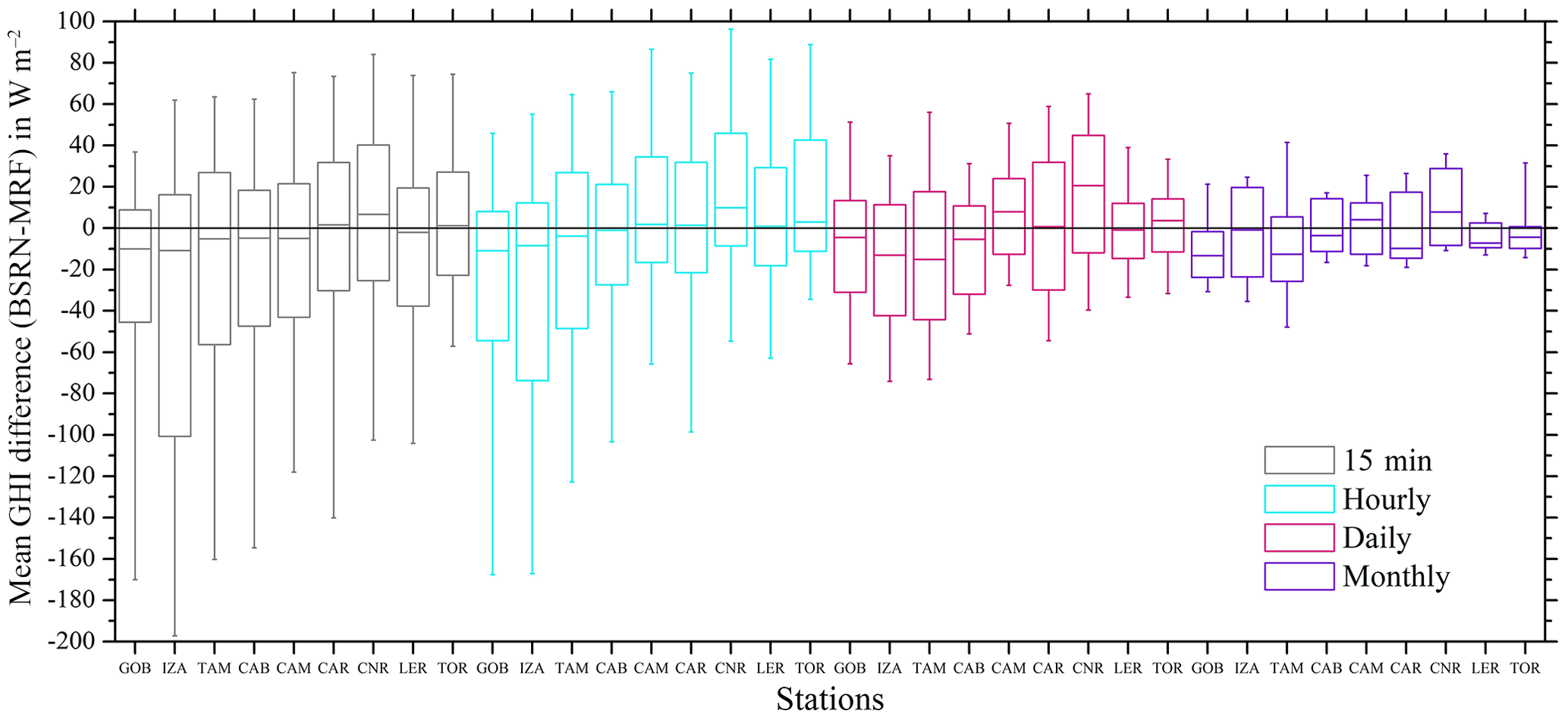
Figure 6Mean GHI differences in W m−2 derived by MRF as compared to the BSRN stations for each time horizon. The boxes represent the 25th and 75th percentiles, while the in-box lines represent the median of the difference of each station. The upper and lower whiskers represent the minimum and maximum error values.
2.2.2 Multi-regression function
The multi-regression function (MRF) technique was developed as an analytical methodology using the RTM outputs, with the aim to provide results as close as possible to the initial (training set) RTM outputs. The advantage in the use of these functions is that they can be executed very rapidly and can be used for real-time SSR determination. In order to achieve that, analytical functions for the SSR should be constructed. In general, SSR is a function of SZA, COT, AOD, AE, SSA, WV and TOC (Appendix A presents the complete list of nomenclature and abbreviations). For the AE and SSA we used monthly climatological values in order to bridge the gap between the operational input availability and the SSR accuracy. However, a preliminary investigation has been performed for the sensitivity of GHI to WV column and TOC. We compared integrated spectral GHI over the entire spectrum for different TOC values and we found a mean difference of only 0.5 % for TOC ranging between 300 and 400 DU. For WV columns ranging between 0.5 and 2 cm we found a mean difference of 3.2 %, although for SZA < 15∘ this difference was higher, up to 5 %. Therefore, we chose to neglect these variables in the first place and use TOC = 350 DU and WV = 0.5 cm for further calculations, considering the differences mentioned above as a scale of error introduced by this approach.
Table 3Values of parameters used for the polynomial function Eq. (3) of the MRF technique for GHI calculations under clear-sky and cloudy-sky conditions.
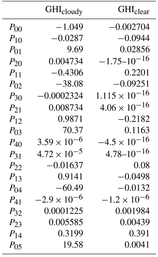
Then, we constructed different polynomial functions according to Gasca and Sauer (2000) for cloudy and clear-sky conditions, to be applied into the scheme presented in Fig. 1. For cloudy cases the irradiance is expressed as f_cloud(SZA, COT) and for clear-sky cases as f_clear(SZA, AOD). We tested different orders of two-variable polynomials to conclude on the best regression (multi-regression analysis) and we found that the estimates closest to the RTM results were achieved using fifth- and fourth-degree polynomials (Sauer and Xu, 1995), as follows:
where x is SZA and y is AOD and COT accordingly (clear- or cloudy-sky pixels). Table 3 presents the analytical values of pxx for the purposes of this study (GHI) under clear- and cloudy-sky conditions. By this approach RTM simulations of SSR are derived in computational times that can be applied in any real-time application.
2.2.3 Neural network
As presented in Taylor et al. (2015), the LUT approach, despite its large size, still provides estimates at discrete input values. The interpolation techniques to correct the input-output parameter intervals are computationally more costly than a continuous function-approximating model, or a NN model, which is more preferable for producing real-time outputs (Hornik et al., 1989). Indicatively, using a test set of 1000 RTM simulations from the developed LUT, we applied an interpolating function to adjacent/nearest value and found that each interpolation calculation required a time in excess (in total ≈ 21 h) of each single run of RTM used to generate the LUT in the first place (≈ 12 h for 1000 RTM simulation outputs with spectral resolution of 1 nm in the range 285–2700 nm), while for the same test set the NN needed almost 0.144 s to generate the 1000 output spectra. Takenaka et al. (2011) have pointed out that the inclusion of many parameters (we incorporated six for the clear-sky and four for the cloudy-sky simulations) and small step sizes (we produced more than 2.5 million RTM simulations in total) can dramatically increase the LUT volume, while Sauer and Xu (1995) and Gasca and Sauer (2000) noted that the multidimensional nature of the dataset requires interpolation/extrapolation procedures that impact strongly on calculation speed. Hence, based on the developed LUT, we trained two sets of NNs, each one consisting of a clear-sky- and a cloudy-sky-specific NN. For multivariate input–output data, feed-forward NNs with a minimum of one layer of “hidden” neurons whose activation functions are nonlinear hyperbolic tangent functions or other general nonlinear sigmoidal functions have been shown in the literature to be a universal function approximator (Cybenko, 1989; Hornik et al., 1989). The input–output vectors used in this study were connected via two network layers – the first containing hidden neurons with tanh activation functions and the second containing output neurons with linear activation functions. The exact mathematical equation relating the NN outputs to the NN inputs for this type of NN is given in the following matrix equation described analytically in Taylor et al. (2014):
The multiplication of the matrix IW1,1 and the vector X is a dot product equivalent to the summation of all input connections to each neuron in the hidden layer. This equation is the continuous and nonlinear functional approximation that relates the output vector to the input vector. This NN approach, its training procedure and all the technical details are described analytically in Taylor et al. (2015).
In the first NN set, we produced instantaneous SSR spectra of the order of 1 million in less than 1 min, using as operational inputs the CAMS AOD 1-day forecasts, the MSG COT and real-time calculations of SZA. The output resolution is high in terms of spectral (1 nm), spatial (0.05∘) and temporal (15 min) components (Taylor et al., 2015), and, operationally speaking, this spectrally based NN (NNS) can incorporate additional inputs as described in Sect. 2.2.1. Similar studies on the temporal variability of SSR by means of spectral representations and the wavelengths absorption parameterization applied to satellite channels and spectral bands were performed by Gasteiger et al. (2014) and Belgulescu et al. (2016). For the purposes of this study we used monthly climatological values for the rest of the input parameters, more specifically TOC from OMI (2007–2016), WV from the Medium Resolution Imaging Spectrometer (MERIS) on board ESA's Environmental Satellite (ENVISAT), and AE and SSA from the AeroCom database (Kinne et al., 2006). The second NN set was trained using integrated SSR over the whole wavelength range using the LUT's spectral data. The SSR results of this technique (called hereafter NN) are more accurate in terms of GHI, DNI and diffuse horizontal irradiance (DHI), as will be discussed in the following section. On the other hand, spectrally weighted products like the UV index, photosynthetically active radiation (PAR) or the vitamin D effective dose (VDED) cannot be produced with this approach, as only the NNS is able to produce the spectral irradiance needed for such applications.
Since the proposed modelling techniques (MRF, NN and NNS) operate in real time, the potential applicability for short-term forecasting purposes for the next few hours is feasible. In this direction, the CAMS AOD is already an operational forecast input (Benedetti et al., 2009), with accurate predictions every 1 h even under high aerosol load conditions (Kosmopoulos et al., 2017). On the other hand, the MSG COT short-term forecasting requires the employment of a cloud motion vector analysis (e.g. Hammer et al., 1999) in high spatial and temporal resolution (5 km × 5 km and 15 min, which is the MSG/SEVIRI resolution) in order to predict the impact of clouds on SSR for the next 2–3 h, while under cloudless conditions the SZA and AOD are the main solar irradiance attenuators and hence are available as input information to the models.
3.1 Performance of real-time techniques
3.1.1 Comparison with RTM
This section initially summarizes the performance of all the real-time modelling techniques against the RTM simulations for all BSRN stations. Figure 3 presents the percentage difference between the RTM simulations and the MRF, NN and NNS techniques. All data presented here are GHI model outputs with a 15 min temporal resolution. The box plots represent the interquartile range between the 25th and 75th percentiles with the in-box line to show the median and the upper and lower whiskers to represent the maximum and minimum error values that are within 1.5× the interquartile range of the box edges. The largest differences for all techniques occur for LER and TOR stations followed by CAB, indicating higher introduced uncertainties over highest latitudes, as observed on the MSG Earth view edges. However, differences for MRF are much smaller for these three stations. For all stations MRF shows differences around zero, showing quite efficient representation of the LUT-based RTM simulations. For the altitude correction (described in Sect. 2.2.1) we included corrections of 4.2 % per kilometre at 20∘ SZA up to 12 % per kilometre at 80∘ (Fig. 4), based on libRadtran model sensitivity analysis.
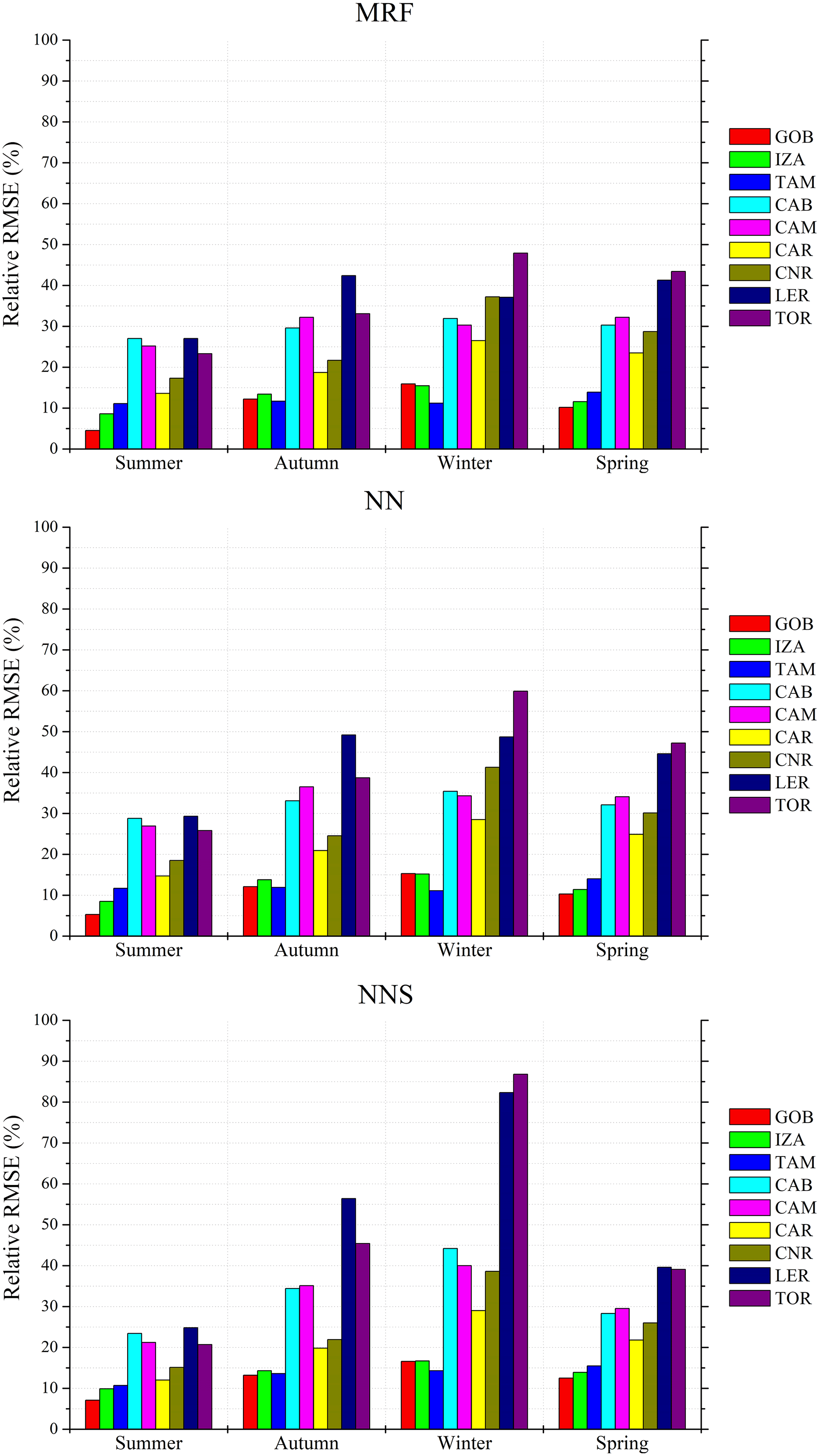
Figure 7Seasonal relative RMSE values of the GHI estimations produced by the real-time techniques as compared to the BSRN measurements.
The NN and NNS approaches showed a systematic underestimation for the NN of ∼ 8 %, while NNS had comparatively the worst performance, with differences in the range of −15 to 80 % (LER station – for the interquartile ranges). The median differences range from −15 to 15 % for NNS and ∼ 5 to 6 % for NN, while they are less than 1 % for MRF. It is clear that spectral output methods (NNS) provide more detailed information (e.g. for specialized studies on spectral impacts on the yield of different PV technologies; Dirnberger et al., 2015; Ishii et al., 2013), but they are more uncertain than the NN and MRF that produce integrated SSR.
3.1.2 Verification with BSRN
The model accuracy was verified against nine BSRN stations. We calculated the regression of the mean GHI between the ground measurements and the model outputs, shown in Fig. 5. We also show the intra-model regression compared to the initial RTM simulations (Fig. 5a) in order to assess the NN and NNS included interpolations of the LUT outputs and the MRF performance. We found that the MRF technique presents identical values to the RTM, for all ground stations and under all climatological conditions. The NN and NNS show quite good agreement too in terms of absolute values, as under all conditions mean GHIs are less than 5 % different from the BSRN measurements. In Fig. 5b we confirmed the similarity of MRF with RTM and in some cases with the NN models, indicating the overall efficiency of all interpolation and multi-function techniques used. A slightly better performance was observed for higher mean GHIs, proving the usefulness under high solar energy potential conditions.
Table 4GHI evaluation results as a function of season and real-time techniques for all stations. The model MBE and RMSE statistical scores are shown in absolute units (W m−2) and as relative magnitude (percentages in brackets).
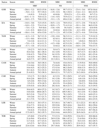
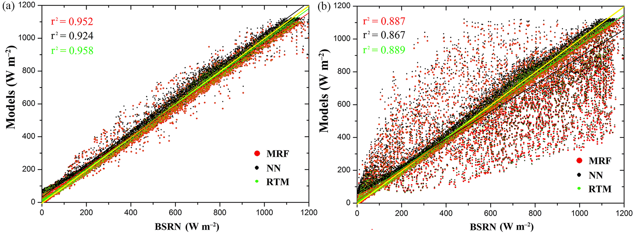
Figure 8Scatterplots of real-time (MRF and NN) and RTM-simulated GHI in W m−2 as compared to the BSRN measurements for all stations under clear-sky (a) and all-sky (clear-sky and cloudy) conditions (b).
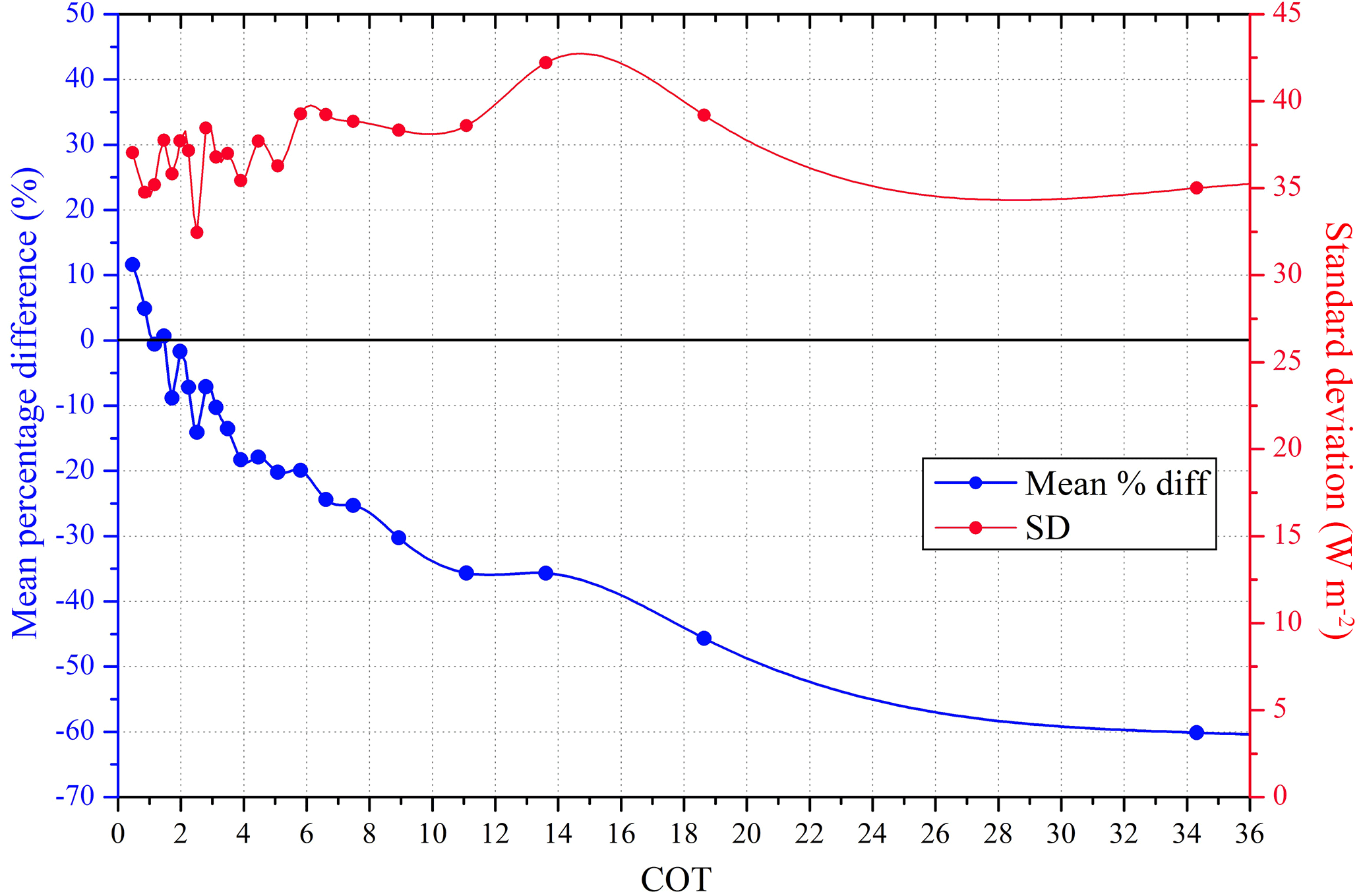
Figure 9Mean percentage difference (blue) and standard deviation (red) of the 15 min GHI produced from the MRF technique as compared to ground-based measurements from all stations as a function of the COT.
Figure 6 shows the accuracy of MRF, being the most reliable technique as presented in Fig. 3, with respect to the ground-based measurements for various temporal integrations, starting from the (actual derived) 15 min to hourly, daily and monthly averages. The uncertainty range of the MRF simulations given as mean interquartile GHI differences is highest (from −100 to 40 W m−2, depending on the station) for the 15 min resolution. It is reduced for hourly and daily averages (−70 to 40 and −40 to 30 W m−2, respectively) and is minimized for the monthly averages (−20 to 20 W m−2). In particular, IZA and TAM showed the highest differences for all temporal retrievals, while LER and TOR presented minimum differences down to ±20 W m−2 for the interquartile range of the 15 min averages. The median values are within 10 W m−2 for the 15 min and hourly resolutions, while the corresponding minimum and maximum error values (represented in Fig. 6 as the upper and lower whiskers) extend from −200 to 100 W m−2 for the aforementioned resolutions and are reduced to ±60 and ±40 W m−2 for the daily and monthly averages, respectively. These results are comparable with similar model verification approaches and studies (Riihela et al., 2015; Muller et al., 2015; Thomas et al., 2016; Eissa et al., 2015a, b). Indicatively, Muller et al. (2015) and Riihela et al. (2015) discussed the CM-SAF SARAH (Solar surfAce RAdiation Heliosat) data record, which consists of post-processed data. They calculated a mean monthly error for GHI of 5.5 W m−2 and a mean daily error of 12.1 W m−2, with additional uncertainties in terms of spatial representativeness and measurement quality of about ±12 W m−2, while they did not provide relevant information about the hourly or even higher time resolution. The overall accuracy of all models was also evaluated with respect to seasonality. In Fig. 7 we present the seasonal rRMSE values of the GHI estimations produced by the MRF, NN and NNS models as compared to the BSRN 15 min interval measurements. The rRMSE for MRF ranges from 5 to 48 % for GOB and TOR stations, respectively; for NN the range increases to 6–60 %; and for NNS the corresponding range is 7–87 %. We need to note that the aforementioned large differences correspond to significantly low absolute GHI values, indicating the impact under cloudy conditions mainly in the winter season, at stations with high mean cloudiness (LER, TOR, CAM and CAB). In the summer, results are better for all stations and for all models (5–29 %), while GOB, IZA and TAM stations showed the lowest rRMSE values (5–12 % in summer and 12–17 % in winter), linked with their lower cloudiness. Eissa et al. (2015a, b) validated the HelioClim-3 database and the McClear model in Egypt and in the United Arab Emirates, and they found RMSE of 68.4–151.7 and 22–47 W m−2, respectively (we found a range of 58.2–70.8 W m−2). Thomas et al. (2016) validated the latest version of HelioClim-3 (v5) against BSRN and found rRMSE of 14.1–37.2 % for the 15 min averages, which is directly comparable to our 15 min results (12–35.7 %). In particular, for the LER, TOR, CAB, CAM, CAR and TAM stations they found rRMSE of 37.2, 33, 29.4, 25.9, 16.3 and 15.8 %, while from our MRF performance evaluation results we observe 35.7, 35.6, 29.9, 30.3, 20.2 and 12.2 % for the same stations. This indicates that the use of the suggested real-time modelling techniques enables the production of instantaneous, high-resolution and quite accurate (as compared to the post-processed databases) GHI outputs that can be used for solar-energy-related applications and studies. A detailed presentation of results for all metrics and stations can be found in Table 4.
3.2 Sensitivity analysis
3.2.1 Cloud effect
The cloud effect via the radiative transfer of solar radiation in the atmosphere represents the greatest source of uncertainty in the simulation of SSR, while several models do not have the capability to deal with clouds coexisting with a radiatively active atmosphere (Cahalan et al., 2005). Small changes in cloudiness and its optical properties can impact on GHI. The magnitude of the cloud effects on the model to BSRN comparison can be seen in Fig. 8. Under clear-sky conditions (Fig. 8a), the regression of the 15 min modelled GHI values, in terms of coefficient of determination (r2), shows very good agreement when compared with the BSRN measurements for both MRF (0.952) and NN-based (0.924) techniques. We plotted the RTM simulations as well in order to depict the corresponding regression (0.958). The distinct scatter shown under all-sky conditions (Fig. 8b) with the cloud cases linked with an underestimation of the modelled GHI in comparison to the BSRN values, while the corresponding r2 decreased to 0.887 and 0.867 for the MRF and NN techniques, respectively (the RTM was almost identical to the MRF, i.e. r2= 0.889). This effect has to do with the MSG COT uncertainties and hence introduces errors into the outputs of the SSR techniques (Derrien and Le Gléau, 2005; Pfeifroth et al., 2016). In addition, comparison principles of (point) station GHI measurements with a 0.05∘ MSG cloud “picture” are responsible for part of the observed deviations. As an example, for instants in which the MSG 0.05∘ grid is partly cloudy, the BSRN GHI measurements could fluctuate more than 100 %, depending on whether the sun is visible or whether clouds attenuate the direct component of the solar irradiance. As a result, in the case of a partly covered 0.05∘ pixel and in the absence of clouds between the BSRN instrument and the sun, BSRN-measured GHI would be much higher than the modelled one. Of course, the opposite situation is feasible as well, consequently causing an overestimation of the modelled GHI (Koren et al., 2007).
Figure 9 illustrates the mean percentage difference and standard deviation of the 15 min GHI produced by the MRF and the measured values by the BSRN stations (only instances with cloudy conditions were used for all stations) as a function of COT. For COT < 2, the MRF technique results in higher GHI values than those actually measured, 1–12 %, while as the COT values increase the MRF underestimates the measurements by up to −60 % for COT around 35. We note that under such high COT values the mean radiation values are much lower than 50 W m−2. The standard deviation reaches its highest value of 43 W m−2 for COT 14–16, while its lowest value of 32 W m−2 is found for COT 2.6.
3.2.2 Aerosol effect
In addition to the clouds, aerosols play an important role in the solar radiation transfer in the atmosphere. Especially in places with high solar energy potential, where cloud-free conditions prevail during the greater part of the year, significant aerosol sources could exist (Gkikas et al., 2012). The aerosols effect is closely related to the aerosol optical properties and mostly AOD, and as a consequence the uncertainty in the model AOD input could result in significant errors in the assessment of SSR (Oumbe et al., 2015; Kosmopoulos et al., 2017). For the purposes of this study we used the Global Atmosphere Watch (GAW-PFR) station of IZA, which is an internationally recognized test bed for aerosol remote sensing instruments (Cuevas et al., 2016), to quantify the AOD difference between the operational input from CAMS and a PFR instrument, under high-altitude conditions (Garcia et al., 2013). In Fig. 10 we present the yearly frequency distribution of the differences between CAMS and PFR values for cloudless sky conditions. The majority of the AOD differences are lower than 0.2, with the maximum frequency encountered at zero AOD differences, indicating the overall good accuracy of CAMS-derived 1-day forecasts of AOD. The mean absolute difference was found equal to 0.1075 ± 0.1038 (1σ). This shows an overestimation of 0.1 for CAMS that could lead to a small MRF GHI underestimation of 2 % compared with BSRN measured GHI. Finally, in Fig. 11 a scatterplot of the CAMS-PFR differences in AOD is shown as a function of absolute differences in GHI derived between the MRF technique and the IZA measurements. The GHI differences are spread around zero independently of the AOD difference, showing the negligible dependence of such small AOD differences on the GHI model calculations.
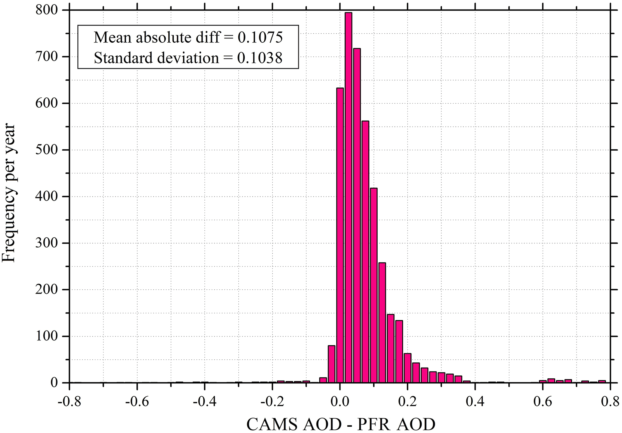
Figure 10Frequency histogram of differences between the CAMS and the PFR AOD at the Izaña station together with the mean absolute difference and standard deviation metrics.
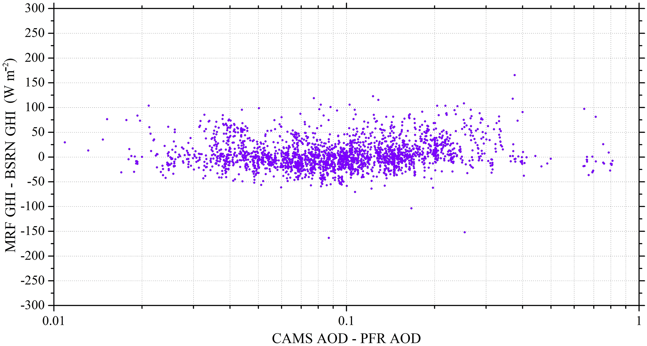
Figure 11Absolute differences in GHI (in W m−2) derived by the MRF technique from the ground-based measurements at Izaña (BSRN pyranometer), as a function of differences in AOD from CAMS and PFR.
This study proposed state-of-the-art modelling techniques (NNS, NN, MRF) for the real-time estimation of SSR, which have been validated against ground-based BSRN measurements. The determination and understanding of the input parameter effects on radiative transfer revealed that the accuracy of simulations depends on the quality and resolution of the atmospheric inputs to the models (mostly COT and AOD), while increasing the calculation speed and including spectral GHI information decreases the model accuracy.
We firstly described the developed modelling techniques, which are based on large LUTs for clear-sky and cloudy conditions. Verification of these models was performed for the GHI against ground measurements at nine stations, with variable geographical, atmospheric and altitudinal conditions. The comparison showed a dependence on seasonal variability, with summer rRMSE values below 30 % for all models and under all conditions, and revealed largest errors for the NNS technique because of the spectral special characteristics, as well as for LER and TOR stations. The NN presented a slight underestimation of 8 % against its training RTM simulations, while against BSRN stations it achieved MBE and RMSE values less than 30 and 80 W m−2, respectively, for the annual period, indicating relatively good agreement under various conditions. The technique with the most accurate results, which was almost identical to the RTM simulations, was MRF. Under different temporal scales the mean GHI differences in terms of 25th to 75th interquartiles, compared to the nine stations, were found to range from −100 to 40 W m−2 for the 15 min intervals, −70 to 40 W m−2 for the hourly means, and −40 to 30 and −20 to 20 W m−2 for the daily and monthly averages, and they were almost 10 W m−2 for the median of difference of each station.
The results presented here show the potential use of such techniques for solar-energy-related applications and electricity grid support services (IRENA, 2015). Comparison of the proposed real-time models with existing databases (e.g. SARAH), which in most cases are post-processed data using past data series, showed similar results. Finally, we tested the impact of cloud and aerosol inputs to the models in order to reveal the AOD forecast accuracy of CAMS, which turned out to be ∼ 0.1 in absolute terms as compared to ground-based sun-photometric measurements in Izaña. The CAMS AOD performance has also been tested under high aerosol loads (Kosmopoulos et al., 2017) in different regions (e.g. the eastern Mediterranean), showing similar results compared with MODIS. However, its accuracy should be checked in the case of application of the methodology to different regions (e.g. Middle East). The MSG COT is related to MRF underestimation of the order of 60 % under highly cloudy conditions (COT > 30) and negligible GHI levels (< 50 W m−2). As a result, the presented real-time models based on the synergy of satellite products, RTM and NN or MRF techniques, are a promising tool to be used within the solar-energy-related community. Improvements on satellite-based model inputs from latest and future satellite missions (e.g. Sentinel missions) could be implemented in the future in the existing system in order to improve spatial and temporal resolution and GHI accuracy.
All data sets used and produced for the purposes of this paper are freely available and can be requested from the corresponding author. The model codes developed (NN, NNS and MRF) can be used for various applications after consultation with the corresponding author.
| AE | Ångström exponent |
| AOD | Aerosol optical depth |
| BSRN | Baseline Surface Radiation Network |
| CAMS | Copernicus Atmosphere Monitoring Service |
| CM SAF | Satellite Application Facility on Climate Monitoring |
| COT | Cloud optical thickness |
| CP | Cloud phase |
| CSP | Concentrated solar power |
| CT | Cloud type |
| DHI | Diffuse horizontal irradiance |
| DNI | Direct normal irradiance |
| DU | Dobson unit |
| EDGAR | Emission Database for Global Atmospheric Research |
| ENVISAT | Environmental Satellite |
| EO | Earth observation |
| ESA | European Space Agency |
| EU | European Union |
| GAW | Global Atmosphere Watch |
| GHI | Global horizontal irradiance |
| ICOT | Ice cloud optical thickness |
| libRadtran | Library for Radiative transfer |
| LUT | Look-up table |
| MACC | Monitoring Atmospheric Composition and Climate |
| MBE | Mean bias error |
| MENA | Middle East and North African countries |
| MERIS | Medium Resolution Imaging Spectrometer |
| MODIS | Moderate Resolution Imaging Spectroradiometer |
| MRF | Multi-regression function |
| MSG | Meteosat Second Generation |
| NN | Neural network |
| NNS | Neural network spectral |
| OMI | Ozone Monitoring Instrument |
| PAR | Photosynthetically active radiation |
| PFR | Precision filter radiometer |
| PV | Photovoltaic |
| rMBE | Relative mean bias error |
| RMSE | Root mean square error |
| rRMSE | Relative root mean square error |
| RTM | Radiative transfer model |
| SAFNWC | Satellite Application Facilities for NoWCasting |
| SARAH | Solar surfAce RAdiation Heliosat |
| SEVIRI | Spinning Enhanced Visible and InfRared Imager |
| SPEW | Speciated Particulate Emission Wizard |
| SSA | Single-scattering albedo |
| SSR | Surface solar radiation |
| SZA | Solar zenith angle |
| TOC | Total ozone column |
| UV | Ultraviolet |
| VDED | Vitamin D effective dose |
| WCOT | Water cloud optical thickness |
| WV | Water vapour |
The authors declare that they have no conflict of interest.
This article is part of the special issue “SKYNET – the international network for aerosol, clouds, and solar radiation studies and their applications”. It is not associated with a conference.
This research was partly funded by the H2020 GEO-CRADLE project under
grant agreement no. 690133, the IERSD/NOA's action THESPIA with grant number
PDE2013SE01380031 under the call KRIPIS, and the project
Aristotelis-SOLAR.
Edited by: M. Campanelli
Reviewed by: three anonymous referees
Aebi, C., Gröbner, J., Kämpfer, N., and Vuilleumier, L.: Cloud radiative effect, cloud fraction and cloud type at two stations in Switzerland using hemispherical sky cameras, Atmos. Meas. Tech., 10, 4587–4600, https://doi.org/10.5194/amt-10-4587-2017, 2017.
Benedetti, A., Moncrette, J. J., Boucher, O., Dethof, A., and the GEMS-AER team: Aerosol analysis and forecast in the ECMWF Integrated Forecast System. Part II: Data assimilation, J. Geophys. Res., 114, D13205, https://doi.org/10.1029/2008JD011115, 2009.
Bengulescu, M., Blanc, P., and Wald, L.: On the temporal variability of the surface solar radiation by means of spectral representations, Adv. Sci. Res., 13, 121–127, https://doi.org/10.5194/asr-13-121-2016, 2016.
Beyer, H. G., Polo Martinez, J., Suri, M., Torees, J. L., Lorenz, E., Muller, S. C., Hoyer-Klick, C., and Ineichen, P.: Report on benchmarking of radiation products, Report under no 038665 of MESoR, available at: http://www.mesor.net/deliverables.html (last access: 27 July 2017), 2009.
Cahalan, R., Oreopoulos, L., Marshak, A., Evans, F., Davis, A., Pincus, R., Yetzen, K. H., Mayer, B., Yetzer, K. H., Mayer, B., Davies, R., Ackerman, T. P., Barker, H. W., Clothiaux, E. E., Ellingson, R. G., Garay, M. J., Kassianov, E., Kinne, S., Macke, A., O'Hirok, W., Partain, P. T., Prigarin, S. M., Rublev, A. N., Stephens, G. L., Szczap, F., Takara, E. E., Varnai, T., Wen, G., and Zhuravleva, T.: The I3RC: Bringing Together the Most Advanced Radiative Transfer Tools for Cloudy Atmospheres, B. Am. Meteorol. Soc., 86, 1275–1293, 2005.
Cuevas, E., Guirado, C., Barreto, A., Garcia, R., Garcia, O., Schneider, M., Romero-Campos, P. M., Almansa, F., Lopez-Solano, J., Rodondas, A., and Ramos, R.: WMO-CIMO Testbed for Aerosols and Water Vapor Remote Sensing Instruments (Izana, Spain), World Meteorological Organisation, CIMO TECO 2016, Madrid, Spain, 27–30 September 2016.
Cybenko, G.: Approximation by super-positions of a sigmoidal function, Math. Control Signal., 2, 303–314, 1989.
Dahlback, A. and Stamnes, K.: A new spherical model for computing the radiation field available for photolysis and heating at twilight, Planet. Space Sci., 39, 671–83, 1991.
Dee, D. P. and Uppala, S.: Variational bias correction of satellite radiance data in the ERA-Interim reanalysis, Q. J. Roy. Meteor. Soc., 135, 1830–1841, https://doi.org/10.1002/qj.493, 2009.
Deneke, H. and Feijt, A.: Estimation surface solar irradiance from METEOSAT SEVIRI-derived cloud properties, Remote Sens. Environ., 112, 3131–3141, 2008.
Derrien, M. and Le Gleau, H.: MSG/SEVIRI cloud mask and type from SAFNWC, Int. J. Remote Sens., 26, 4707–4732, 2005.
Dirnberger, D., Blackburn, G., Müller, B., and Reise, C.: On the impact of solar spectral irradiance on the yield of different PV technologies, Sol. Energ. Mat. Sol. C., 132, 431–442, 2015.
Dorvlo, A. S. S., Jervase, J. A., and Lawati, A. A.: Solar radiation estimation using artificial neural networks, Appl. Energ., 71, 307–319, 2002.
EC: Science Comminucation Unit, University of the West of England, Bristol (2012), Science for Environment Policy Future Brief: Earth Observation's Potential for the European Commission DG Environment, available at: http://ec.europa.eu/science-environment-policy (last access: 25 March 2017), 2013.
Eck, T. F., Holben, B. N., Slutsker, I., and Setzer, A.: Measurements of irradiance attenuation and estimation of aerosol single scattering albedo for biomass burning aerosols in Amazonia, J. Geophys. Res., 103, 31865–31878, 1998.
Eissa, Y., Munawwar, S., Oumbe, A., Blanc, P., Ghedira, H., Wald, L., Bru, H., and Goffe, D.: Validation surface downwelling solar irradiances estimated by the McClear model under cloud-free skies in the United Arab Emirates, Sol. Energy, 114, 17–31, 2015a.
Eissa, Y., Korany, M., Aoun, Y., Boraiy, M., Abdel-Wahab, M. M., Alfaro, S. C., Blanc, P., El-Metwally, M., Ghedira, H., Hungershoefer, K., and Wald, L.: Validation of the surface downwelling solar irradiance estimates of the HelioClim-3 database in Egypt, Remote Sens., 7, 9269–9291, https://doi.org/10.3390/rs70709269, 2015b.
Ellingson, R. G., Ellis, J., and Fels, S.: The intercomparison of radiation codes used in climate models: Longwave results, J. Geophys. Res., 96, 8929–8953, 1991.
Emde, C., Buras-Schnell, R., Kylling, A., Mayer, B., Gasteiger, J., Hamann, U., Kylling, J., Richter, B., Pause, C., Dowling, T., and Bugliaro, L.: The libRadtran software package for radiative transfer calculations (version 2.0.1), Geosci. Model Dev., 9, 1647–1672, https://doi.org/10.5194/gmd-9-1647-2016, 2016.
EU Energy Policy to 2050: achieving 80–95 % emmissions reductions, EWEA, The European Wind Energy Association: March, 2011.
Eskes, H., Huijnen, V., Arola, A., Benedictow, A., Blechschmidt, A.-M., Botek, E., Boucher, O., Bouarar, I., Chabrillat, S., Cuevas, E., Engelen, R., Flentje, H., Gaudel, A., Griesfeller, J., Jones, L., Kapsomenakis, J., Katragkou, E., Kinne, S., Langerock, B., Razinger, M., Richter, A., Schultz, M., Schulz, M., Sudarchikova, N., Thouret, V., Vrekoussis, M., Wagner, A., and Zerefos, C.: Validation of reactive gases and aerosols in the MACC global analysis and forecast system, Geosci. Model Dev., 8, 3523–3543, https://doi.org/10.5194/gmd-8-3523-2015, 2015.
Federico, S., Torcasio, R. C., Sanò, P., Casella, D., Campanelli, M., Meirink, J. F., Wang, P., Vergari, S., Diémoz, H., and Dietrich, S.: Comparison of hourly surface downwelling solar radiation estimated from MSG-SEVIRI and forecast by the RAMS model with pyranometers over Italy, Atmos. Meas. Tech., 10, 2337–2352, https://doi.org/10.5194/amt-10-2337-2017, 2017.
Garcia, R. D., Cuevas, E., Cachorro, V. E., Ramos, R., and de Frutos, A. M.: Comparison between Measurements and Model Simulations of Solar Radiation at a High Altitude Site: Case Studies for the Izana BSRN Station, AIP Conf. Proc., 1531, 864, https://doi.org/10.1063/1.4804907, 2013.
Gasca, M. and Sauer, T.: Polynomial interpolation in several variables, Adv. Comput. Math., 12, 377–410, 2000.
Gasteiger, J., Emde, C., Mayer, B., Buras, R., Buehler, S. A., and Lemke, O.: Representative wavelengths absorption parameterization applied to satellite channels and spectral bands, J. Quant. Spectrosc. Ra., 148, 99–115, 2014.
Gleeson, E., Toll, V., Nielsen, K. P., Rontu, L., and Mašek, J.: Effects of aerosols on clear-sky solar radiation in the ALADIN-HIRLAM NWP system, Atmos. Chem. Phys., 16, 5933–5948, https://doi.org/10.5194/acp-16-5933-2016, 2016.
Gkikas, A., Houssos, E. E., Hatzianastassiou, N., Papadimas, C. D., and Bartzokas, A.: Synoptic conditions favouring the occurrence of aerosol episodes over the broader Mediterranean basin, Q. J. Roy. Meteor. Soc., 138, 932–949, 2012.
Green, A., Diep, C., Dunn, R., and Dent, J.: High capacity factor CSP-PV hybrid systems, Energy Proced., 69, 2049–2059, 2015.
Hammer, A., Heinemann, D., Lorenz, E., and Luckehe, B.: Short-term forecasting of solar radiation: a statistical approach using satellite data, Sol. Energy, 67, 139–150, 1999.
Hegner, H., Muller, G., Nespor, V., Ohmura, A., Steigrad, R., and Gilgen, H.: Technical plan for BSRN data management – 1998 update, WMO/TD 882, WCRP/WMO, 38, 1998.
Hess, K., Koepke, P., and Schult, I.: Optical properties of aerosols and clouds: the software package OPAC, B. Am. Meteorol. Soc., 79, 831–844, 1998.
Hornik, K., Stinchcombe, M., and White, H.: Multilayer Feedforward Networks Are Universal Approximators, Neural Networks, 2, 359–366, 1989.
Huang, G., Ma, M., Liang, S., Liu, S., and Li, X.: A LUT-based approach to estimate surface solar irradiance by combining MODIS and MTSAT data, J. Geophys. Res., 116, D22201, https://doi.org/10.1029/2011JD016120, 2011.
IEA: Findings of Recent International Energy Agency Work 2007, http://www.iea.org/publications/freepublications/publication/findings.pdf (last access: 27 May 2016), OECD/IEA, Paris, 2007.
IEA: Electricity information, Published by the International Energy Agency, 762, 2010.
Ineichen, P.: Comparison of eight clear sky broadband models against 16 independent data banks, Sol. Energy, 80, 468–478, 2006.
IPCC: Renewable energy sources and climate change mitigation, Special Report of the IPCC, Cambridge University Press, New York, USA, 2012.
IRENA: Renewable energy integration in power grids, IEA-ETSAP and IRENA Technology brief E15, available at: http://www.irena.org/DocumentDownloads/Publications/IRENA-ETSAP_Tech_Brief_Power_Grid_Integration_2015.pdf (last access: 7 August 2017), 2015.
IRENA: Solar PV in Africa: Costs and markets, available at: https://www.irena.org/DocumentDownloads/Publications/IRENA_Solar_PV_Costs_Africa_2016.pdf (last access: 7 August 2017) 2016.
Ishii, T., Otani, K., Takashima, T., and Xue, Y.: Solar spectral influence on the performance of photovoltaic (PV) modules under fine weather and cloudy weather conditions, Prog. Photovoltaics, 21, 481–489, 2013.
ITA: Renewable Energy Top Markets Report 2016, International Trade Administration of U.S. Department of Commerce (Industry & Analysis), April 2016.
Jager-Waldau, A.: PV status report 2016, JRC Science for Policy Report, 2016.
Kato, S., Ackerman, T., Mather, J., and Clothiaux, E.: The k-distribution method and correlated-k approxiamation for shortwave radiative transfer model, J. Quant. Spectrosc. Ra., 62, 109–121, 1999.
Kinne, S., Schulz, M., Textor, C., Guibert, S., Balkanski, Y., Bauer, S. E., Berntsen, T., Berglen, T. F., Boucher, O., Chin, M., Collins, W., Dentener, F., Diehl, T., Easter, R., Feichter, J., Fillmore, D., Ghan, S., Ginoux, P., Gong, S., Grini, A., Hendricks, J., Herzog, M., Horowitz, L., Isaksen, I., Iversen, T., Kirkevåg, A., Kloster, S., Koch, D., Kristjansson, J. E., Krol, M., Lauer, A., Lamarque, J. F., Lesins, G., Liu, X., Lohmann, U., Montanaro, V., Myhre, G., Penner, J., Pitari, G., Reddy, S., Seland, O., Stier, P., Takemura, T., and Tie, X.: An AeroCom initial assessment – optical properties in aerosol component modules of global models, Atmos. Chem. Phys., 6, 1815–1834, https://doi.org/10.5194/acp-6-1815-2006, 2006.
Koren, I., Remer, L. A., Kaufman, Y. J., Rudich, Y., and Martins, J. V.: On the twilight zone between clouds and aerosols, Geophys. Res. Lett. 34, L08805, https://doi.org/10.1029/2007GL029253, 2007.
Kosmopoulos, P. G., Kazadzis, S., Lagouvardos, K., Kotroni, V., and Bais, A.: Solar energy prediction and verification using operational model forecasts and ground-based solar measurements, Energy, 93, 1918–1930, 2015.
Kosmopoulos, P. G., Kazadzis, S., Taylor, M., Athanasopoulou, E., Speyer, O., Raptis, P. I., Marinou, E., Proestakis, E., Solomos, S., Gerasopoulos, E., Amiridis, V., Bais, A., and Kontoes, C.: Dust impact on surface solar irradiance assessed with model simulations, satellite observations and ground-based measurements, Atmos. Meas. Tech., 10, 2435–2453, https://doi.org/10.5194/amt-10-2435-2017, 2017.
Lara-Fanego, V., Ruiz-Arias, J. A., Pozo-Vazquez, D., Santos-Alamillos, F. J., and Tovar-Pescador, J.: Evaluation of the WRF model solar irradiance forecasts in Andalusia (southern Spain), Sol. Energy, 86, 2200–2217, 2012.
Lefevre, M., Blanc, P., Espinar, B., Gschwind, B., Ménard, L., Ranchin, T., Wald, L., Sabonet, L., Thomas, C., and Wey, E.: The HelioClim-1 database of daily solar radiation at Earth surface: an example of the benefits of GEOSS Data-CORE, IEEE J. Sel. Top. Appl., 7, 1745–1753, 2014.
Lindfors, A. V., Kouremeti, N., Arola, A., Kazadzis, S., Bais, A. F., and Laaksonen, A.: Effective aerosol optical depth from pyranometer measurements of surface solar radiation (global radiation) at Thessaloniki, Greece, Atmos. Chem. Phys., 13, 3733–3741, https://doi.org/10.5194/acp-13-3733-2013, 2013.
Lopez, G., Rubio, M. A., Martinez, M., and Batlles, F. J.: Estimation of hourly global photosynthetically active radiation using artficial neural network models, Agr. Forest Meteorol., 107, 279–291, 2001.
Mayer, B. and Kylling, A.: Technical note: The libRadtran software package for radiative transfer calculations – description and examples of use, Atmos. Chem. Phys., 5, 1855–1877, https://doi.org/10.5194/acp-5-1855-2005, 2005.
Menard, L., Nust, D., Ngo, K. M., Blanc, P., Jirka, S., Maso, J., Ranchin, T., and Wald, L.: Interoperable Exchange Of Surface Solar Irradiance Observations: A Challenge, Energy Proced., 76, 113–120, 2015.
MétéoFrance: Algorithm theoretical basis document for cloud products (CMa-PGE01 v3.2, CT-PGE02 v2.2 & CTTH-PGE03 v2.2), Technical Report SAF/NWC/CDOP/MFL/SCI/ATBD/01, Paris: MétéoFrance, 2013.
Mueller, R. W., Matsoukas, C., Gratzki, C., Behr, H. D., and Hollmann, R.: The CM SAF operational scheme for the satellite based retrieval of solar surface irradiance – A LUT based eigenvector hybrid approach, Remote Sens. Environ., 13, 1012–1024, 2009.
Muller, R., Pfeifroth, U., Trager-Chatterjee, C., Trentmann, J., and Cremer, R.: Digging the METEOSAT Treasure – 3 Decades of Solar Surface Radiation, Remote Sensing 7, 8067–8101, https://doi.org/10.3390/rs70608067, 2015.
NREL: On the path to sunshot, On the Path to SunShot: Emerging Opportunities and Challenges in U.S. Solar Manufacturing, NREL/TP-7A40-65788, available at: https://www.nrel.gov/docs/fy16osti/65788.pdf (last access 14 February 2017), 2016.
Oreopoulos, L. and Mlawer, E.: Nowcast Modeling: the continual Intercomparison of radiation codes (CIRC) assessing anew the quality of GCM radiation algorithms, B. Am. Meteorol. Soc., 91, 3, 305–310, 2010.
Oreopoulos, L., Mlawer, E., Delamere, J., Shippert, T., Cole, J., Formin, B., and Rossow, W. B.: The continual intercomparison of radiation codes: results from phase I, J. Geophys. Res.-Atmos., 117, https://doi.org/10.1029/2011JD016821, 2012.
Oumbe, A., Bru, H., Li, C., Blanc, P., Wald, L., Ghedira, H., and Goffe, D.: Improving the solar resource estimation in the United Arab Emirates using aerosol and irradiance measurements. Proceedings of the ISES Solar World Conference 2015, 200–208, Daegu, South Korea, 2015.
Pfeifroth, U., Kothe, S., and Trentmann, J.: Validation report: Meteosat solar surface radiation and effective cloud albedo climate data record (Sarah 2), EUMETSAT SAF CM Validation report with reference number SAF/CM/DWD/VAL/ METEOSAT/HEL, 2.1, https://doi.org/10.5676/EUM_SAF_CM/SARAH/V002, 2016.
Qu, Z., Oumbe, A., Blanc, P., Espinar, B., Gesell, G., Gschwind, B., Gschwind, B., Kluser, L., Lenevre, M., Sabonet, L., Schroedter-Homscheidt, M., and Wald, L.: Fast radiative transfer parameterisation for assessing the surface solar irradiance: The Heliosat-4 method, Energy Meteorology, 26, 33–57, 2017.
REN21: Renewables global futures report: Great debates towards 100 % renewable energy, available at: http://www.ren21.net/wp-content/uploads/2017/10/GFR-Full-Report-2017_webversion_3.pdf (last access: 21 June 2017), 2017.
Riihela, A., Carlund, T., Trentmann, J., Muller, R., and Lindfors, A.V.: Validation of CM SAF Surface Solar Radiatiin Datasets over Finland and Sweden, Remote Sens. 7, 6663–6682, https://doi.org/10.3390/rs70606663, 2015.
Roebeling, R. A., Feijt, A. J., and Stamnes, P.: Cloud property retrievals for climate monitoring: implications of differences between SEVIRI on METEOSAT-8 and AVHRR on NOAA-17, J. Geophys. Res., 111, 20210, https://doi.org/10.1029/2005JD006990, 2006.
Sauer, T. and Xu, Y.: On multivariate lagrange interpolation, Math Comput., 64, 1147–1170, 1995.
Schroedter-Homscheidt, M., Delamare, C., Heilscher, G., Heinemann, D., Hoyer, C., Meyer, R., Toggweiler, P., Wald, L., and Zelenka, A.: The ESA-ENVISOLAR project: experience on the commercial use of Earth observation based solar surface irradiance measurements for energy business purposes, Sol. Energy Recources Management for Electricity Generation, edited by: Dunlop, E. D., Wald, L., and Suri, M., Nova Science Publishers, 111–124, available at: http://tinyurl.com/hpf8d5g (last access: 12 June 2017), 2006.
Schulz, J., Albert, P., Behr, H.-D., Caprion, D., Deneke, H., Dewitte, S., Dürr, B., Fuchs, P., Gratzki, A., Hechler, P., Hollmann, R., Johnston, S., Karlsson, K.-G., Manninen, T., Müller, R., Reuter, M., Riihelä, A., Roebeling, R., Selbach, N., Tetzlaff, A., Thomas, W., Werscheck, M., Wolters, E., and Zelenka, A.: Operational climate monitoring from space: the EUMETSAT Satellite Application Facility on Climate Monitoring (CM-SAF), Atmos. Chem. Phys., 9, 1687–1709, https://doi.org/10.5194/acp-9-1687-2009, 2009.
Shettle, E. P.: Models of aerosols, clouds and precipitation for atmospheric propagation studies, in: Proceedings of AGARD conference 454 on atmospheric propagation in the UV, visible, IR and MM-region and related system aspects, 1989.
Suárez, R. A. and Nesmachnow, S.: Parallel Computing Applied to Satellite Images Processing for Solar Resource Estimates, CLEI Electronic journal, 15, 4, http://www.scielo.edu.uy/scielo.php?script=sci_arttext&pid=S0717-50002012000300005&lng=es&tlng=en (last access 11 September 2017), 2012.
Takenaka, H., Nakajima, T. Y., Higurashi, A., Higuchi, A., Takemura, T., Pinker, R. T., and Nakajima, T.: Estimation of solar radiation using a neural network based on radiative transfer, J. Geophys. Res., 116, D08215, https://doi.org/10.1029/2009JD013337, 2011.
Taylor, M., Kazadzis, S., Tsekeri, A., Gkikas, A., and Amiridis, V.: Satellite retrieval of aerosol microphysical and optical parameters using neural networks: a new methodology applied to the Sahara desert dust peak, Atmos. Meas. Tech., 7, 3151–3175, https://doi.org/10.5194/amt-7-3151-2014, 2014.
Taylor, M., Kosmopoulos, P. G., Kazadzis, S., Keramitsoglou, I., and Kiranoudis, C. T.: Neural network radiative transfer solvers for the generation of high resolution solar irradiance spectra parameterized by cloud and aerosol parameters, J. Quant. Spectrosc. Ra. 168, 176–192, 2015.
Tegen, I., Lacis, A. A., and Fung, I.: The influence of climate forcing of mineral aerosols from disturbed soils, Nature, 4, 419–422, 1996.
Thomas, C., Wey, E., Blanc, P., Wald, L., and Lefevre, M.: Validation of HelioClim-3 version 4, HelioClim-3 version 5 and MACC-RAD using 14 BSRN stations, Energy Proced., 91, 1059–1069, 2016.
UN: Progress towards the Sustainable Development Goals, Report of the Secretary-General, available at: http://www.un.org/ga/search/view_doc.asp?symbol=E/2017/66&Lang=E (last access: 14 September 2017), 2017.
Wald, L., Tomas, C., Cousin, S., Blanc, P., Merard, L., Homscheidt, M.S., Gaboardi, E., Simeone, E., Heilscher G., Jacques, S., Serpico, S. B., Huld, T., and Dumortier, D.: The project ENDORSE: exploiting EO data to develop pre-market services in renewable energy, edited by: Pillman W., Schade S., and Smits, P., 25th EnviroInfo Conference “Environmental Informatics”, October 2011, Ispra (VA), Italy, Shaker Verlag, Aachen, Germany, 1, 549–556, 2011.
Wandji Nyamsi, W., Arola, A., Blanc, P., Lindfors, A. V., Cesnulyte, V., Pitkänen, M. R. A., and Wald, L.: Technical Note: A novel parameterization of the transmissivity due to ozone absorption in the k-distribution method and correlated-k approximation of Kato et al. (1999) over the UV band, Atmos. Chem. Phys., 15, 7449–7456, https://doi.org/10.5194/acp-15-7449-2015, 2015.
Zarzalejo, L. F., Raminez, L., and Polo, J.: Artificial intelligence techniques applied to hourly global irradiance estimation from satellite derived cloud index, Energy, 30, 1685–1697, 2005.
Zygmuntowska, M., Mauritsen, T., Quaas, J., and Kaleschke, L.: Arctic Clouds and Surface Radiation – a critical comparison of satellite retrievals and the ERA–Interim reanalysis, Atmos. Chem. Phys., 12, 6667–6677, https://doi.org/10.5194/acp-12-6667-2012, 2012.