The Macquarie Island (LoFlo2G) high-precision continuous atmospheric carbon dioxide record

The Southern Ocean (south of 30^∘ S) is a key global-scale sink of carbon dioxide (CO₂). However, the isolated and inhospitable nature of this environment has restricted the number of oceanic and atmospheric CO₂ measurements in this region. This has limited the scientific community's ability to investigate trends and seasonal variability of the sink. Compared to regions further north, the near-absence of terrestrial CO₂ exchange and strong large-scale zonal mixing demands unusual inter-site measurement precision to help distinguish the presence of midlatitude to high latitude ocean exchange from large CO₂ fluxes transported southwards in the atmosphere. Here we describe a continuous, in situ, ultra-high-precision Southern Ocean region CO₂ record, which ran at Macquarie Island (54^∘37^′ S, 158^∘52^′ E) from 2005 to 2016 using a LoFlo2 instrument, along with its calibration strategy, uncertainty analysis and baseline filtering procedures. Uncertainty estimates calculated for minute and hourly frequency data range from 0.01 to 0.05 µmol mol⁻¹ depending on the averaging period and application. Higher precisions are applicable when comparing Macquarie Island LoFlo measurements to those of similar instruments on the same internal laboratory calibration scale and more uncertain values are applicable when comparing to other networks. Baseline selection is designed to remove measurements that are influenced by local Macquarie Island CO₂ sources, with effective removal achieved using a within-minute CO₂ standard deviation metric. Additionally, measurements that are influenced by CO₂ fluxes from Australia or other Southern Hemisphere land masses are effectively removed using model-simulated radon concentration. A comparison with flask records of atmospheric CO₂ at Macquarie Island highlights the limitation of the flask record (due to corrections for storage time and limited temporal coverage) when compared to the new high-precision, continuous record: the new record shows much less noisy seasonal variations than the flask record. As such, this new record is ideal for improving our understanding of the spatial and temporal variability of the Southern Ocean CO₂ flux, particularly when combined with data from similar instruments at other Southern Hemispheric locations.

1 Introduction

Greenhouse gases, such as CO₂ released by human activity, are primarily responsible for global warming over the last century. Hence, understanding the sources, sinks and feedback mechanisms of these gases is essential for managing the anthropogenic impact on the earth's ecosystems. The Southern Ocean and Antarctic regions, remote from significant industrial and terrestrial biosphere activity, are ideally located to measure global-scale changes and long-term trends in the concentrations of these gases. Australia's Commonwealth Scientific and Industrial Research Organisation (CSIRO) focuses its greenhouse gas sampling programme on the Southern Hemisphere, with long-running flask measurements (Francey et al., 1999), currently at eight sites and in situ CO₂ measurements originally using non-dispersive infrared (NDIR) instruments and now mostly using laser-based spectroscopic instruments (four current long-term sites, one shipboard and various campaigns). With continuing innovation in measurement technology and interpretive models, atmospheric measurements can make a significant contribution to detecting possible climate-induced regional changes in carbon uptake, particularly in the crucial Southern Ocean CO₂ sink, as well as to monitor global changes.

The annual basin-scale Southern Ocean carbon flux is generally well constrained (Lenton et al., 2013). However, the seasonality, long-term trend, interannual and regional variability of this flux is still poorly understood, with divergence between the ocean biogeochemical models, oceanic inversions, atmospheric inversions and (sparse) observations. Considering that up to a third of the global anthropogenic CO₂ uptake by oceans occurs in the Southern Ocean (the region south of 44^∘ S) (Lenton et al., 2013), accurate quantification of this sink is key. However, better quantification is limited by the temporal and spatial availability of observations (both ocean pCO₂ and atmospheric CO₂) across the Southern Ocean region.

For ocean pCO₂, techniques exist to extrapolate and map temporally and spatially sparse measurements, but these approaches are limited. Recent work (Ritter et al., 2017) found that, while often agreeing on the sign of broad-scale decadal trends, these methods fail to agree on the magnitude, mean values, interannual variability and regional distribution. Atmospheric CO₂ measurements can be used to estimate ocean fluxes through an inversion methodology, with the potential advantage that they sample the impact of fluxes over a wider region than would be achieved with oceanic pCO₂ measurements. However, most atmospheric measurements from this region are flask samples, and previous work (Law et al., 2008) has shown that the Southern Ocean flux trends calculated by inversions are sensitive to atmospheric CO₂ data quality. Lenton et al. (2013) also noted that, when observational data were sparse, CO₂ inversion results were highly sensitive to data quality and the number of regions used in the inversion. As such, the addition of a new in situ data record, like that outlined in this paper, should significantly improve future attempts to quantify the Southern Ocean CO₂ sink.

With few representative locations suitable for measuring atmospheric CO₂ in the Southern Ocean, Macquarie Island (54^∘37^′ S, 158^∘52^′ E) was recognised as a potential monitoring location in the 1970s. The island is ideally situated in the middle of the Southern Ocean near the subantarctic front, the boundary between the subantarctic zone and polar frontal zone. This is a highly active oceanic region, known to be a CO₂ sink in the summer months due to biological production, and a CO₂ source in some areas during winter as a result of deepwater mixing (Lenton et al., 2013).

A key challenge when measuring atmospheric CO₂ at Macquarie Island is the limited access. In situ monitoring of atmospheric CO₂ was attempted in 1979 but the restricted access to the island limited the supply of calibration and reference gases. This, along with the intermittent operation of the NDIR, contributed to observations of insufficient quality to be scientifically useful. Macquarie Island was included in CSIRO's flask-sampling network in 1986, with data regularly submitted to international archives from 1990. However, long delays between collection and measurement for flask samples at locations resupplied only once per year along with instrument performance at the time limited their accuracy (Cooper et al., 1999; Sturm et al., 2004). Consequently a new LoFlo in situ CO₂ instrument was installed at Macquarie Island in 2005 (LoFlo2G), taking advantage of technological advances to significantly improve instrument performance, cylinder stability and calibration strategies. While the performance of the instrument has been outstanding (see below), uncertainty about future logistical and staffing constraints at Macquarie Island necessitated decommissioning of the LoFlo instrument in late 2016. It has been replaced with a more linear spectroscopic instrument, which provides comparable precision, needs less frequent calibration and requires lower maintenance. While the LoFlo operated the Macquarie Island, LoFlo was part of a Southern Hemisphere LoFlo network comprising instruments at Cape Grim, Tasmania (144.7^∘ E, 40.7^∘ S), Amsterdam Island (77.5^∘ E, 38.0^∘ S) and Baring Head, New Zealand (174.9^∘ E, 41.4^∘ S). A further LoFlo instrument (LoFlo2B) based at CSIRO (Aspendale, Australia) is used for calibration and related tasks, as well as occasional monitoring of local air.

This paper focuses on the technical aspects of the Macquarie Island in situ CO₂ measurement programme, including site details, instrumentation and calibration (Sects. 2 and 3), data characteristics and comparison with the flask record (Sect. 4). Data selection for baseline conditions is considered in Sect. 5, while Sect. 6 gives a general climatology of the CO₂ data set.

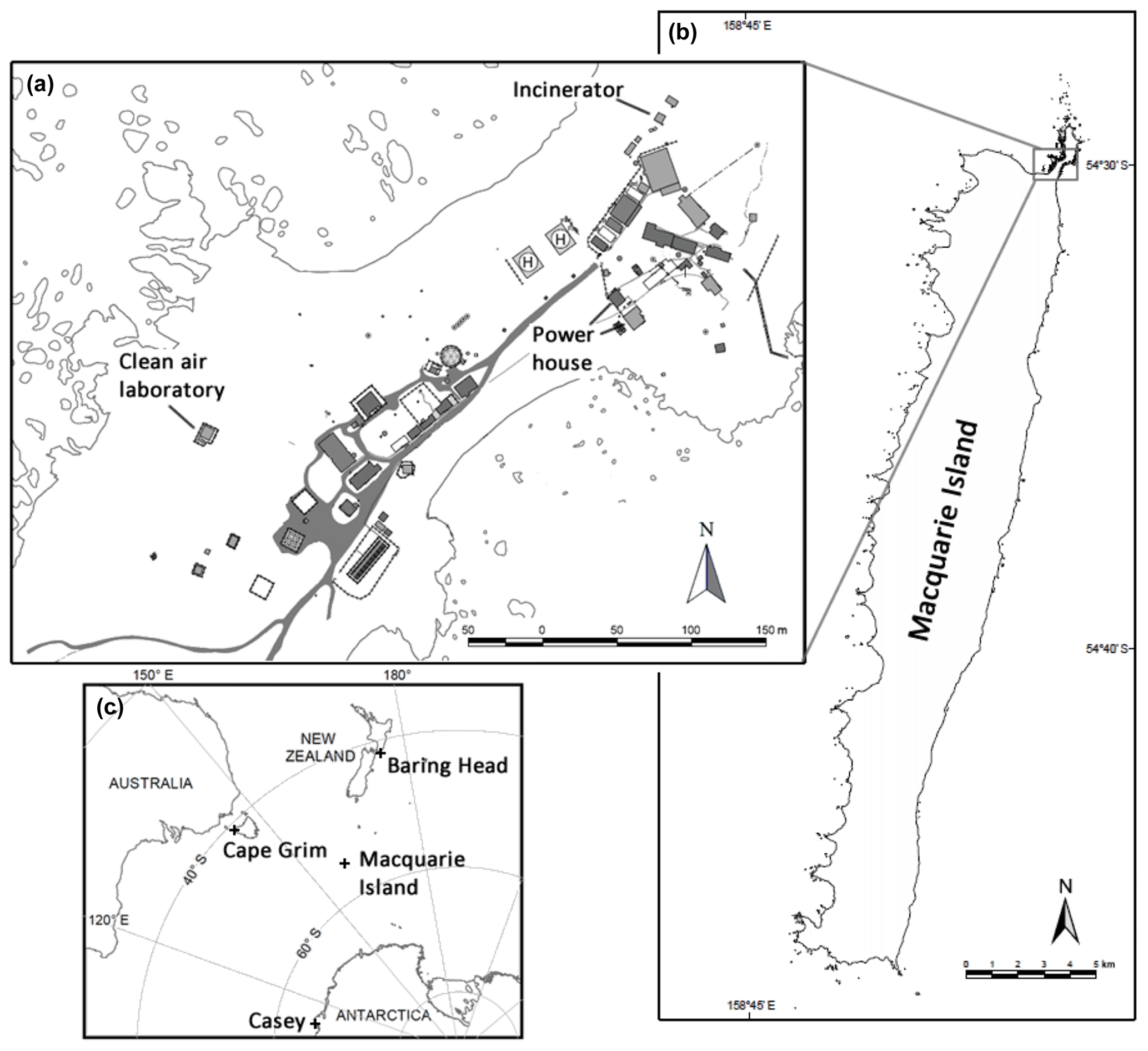
Figure 1 Macquarie Island isthmus map (a) showing the position of the clean-air laboratory, power houses, incinerator and other station buildings; map of the whole of Macquarie Island (b) and Southern Ocean in situ CO₂ measurement stations (c).

2 Site description

Macquarie Island is 34 km long and 5 km wide at its widest point (Russ and Terauds, 2009) (Fig. 1b). It lies on a north–south axis and has an area of 12 788 hectares. Located approximately 1500 km south-east of Australia and 1600 km north of the Antarctic continent, it is ideally situated for Southern-Ocean-based studies (Fig. 1c). Macquarie Island has mean minimum and maximum temperatures of 3.1 and 6.6 ^∘C and an average annual rainfall of 981.6 mm (http://poama.bom.gov.au/climate/dwo/IDCJDW9204.latest.shtml, last access: 5 February 2019). Winds are predominantly from the west (35 %), north-west (35 %) and north (15 %), with an average wind speed greater than 9 m s⁻¹. The island is extremely windy with the winds classed as calm less than 1 % of the time. Macquarie Island is a Global Atmosphere Watch regional site with station identification code MQA.

The clean-air laboratory is located on a low-lying (6 m a.s.l.) isthmus between the main body of the island (a plateau 200–400 m a.s.l.) and a small hill at the northern end of the island (Fig. 1a). It is ∼ 150 m from the residential section of the station, west (upwind) of local anthropogenic point sources of CO₂ (the incinerator and powerhouses, Fig. 1a). The area surrounding the laboratory is highly biologically active and rich in both aquatic and terrestrial flora and fauna, which, considering the relatively low intake height (13 m a.s.l.), may impact CO₂ measurements under low wind speed conditions. A heated concrete floor helps to maintain the laboratory at 19 ^∘C, but on warm sunny days this may drift slowly by 1 to 2^∘.

Maintaining an in situ instrument on Macquarie Island is logistically challenging. Since there is no airport, access has been restricted to an annual resupply voyage in March or April. All instrument servicing must be completed in the “resupply window”, which is generally less than a week. As the resupply ship cannot dock on the island, all equipment and personnel must be transported from the ship to the shore by either helicopter or small boat. These restrictions make Macquarie Island less accessible than many Antarctic sites, possibly the most inaccessible of all sites in the current CO₂ monitoring network. Between resupply visits, Bureau of Meteorology observational and technical staff were responsible for flask sampling and general maintenance of the in situ instrument and drying system. Instrument diagnostics and calibration runs were performed remotely. All communication with the island is via a restricted satellite link.

The clean-air laboratory also houses an atmospheric radon monitor, the output of which can be useful for interpreting the CO₂ record. A 700 L dual-flow-loop two-filter radon detector (Whittlestone and Zahorowski, 1998; Chambers et al., 2014) was installed during the 2011 resupply visit. The detector samples ambient air from an inlet approximately 5 m a.g.l. at a flow rate of ∼ 45 L min⁻¹. A 400 L delay volume was incorporated within the inlet line to allow for the decay of the short-lived radon isotope thoron (²²⁰Rn, $T_{\mathrm{1}/\mathrm{2}}=\mathrm{56}$ s). The detector has a response time of around 45 min and a lower limit of determination (defined here as the radon concentration at which the detector's counting error is 30 %) of ∼ 40 mBq m⁻³. During routine operation the detector is calibrated monthly by being injected with radon from a well-characterised Pylon Radium-222 source (²²⁶Ra, 19.58 kBq ± 4 %) for 6 h at a low rate of ∼ 170 cc min⁻¹, and instrumental background checks are performed quarterly. Problems that arose with the calibration unit and sampling stack blower, which were not able to be addressed until subsequent resupply visits, have limited the data availability and accuracy of the absolute calibration until April 2013.

3 Experimental design and instrumentation

3.1 Continuous CO₂ Instrumentation

Carbon dioxide mole fractions have been measured from April 2005 to October 2016 using a CSIRO LoFlo Mark2 CO₂ analyser. This analyser is an integrated system constructed around a Li-COR (LI-6262, Li-COR Inc., Nebraska, USA) NDIR optical bench. The early design of this system is described in Da Costa and Steele (1999), while details of subsequent calibration strategy and software control development are documented in Francey et al. (2004). The internal Li-COR analyser is operated in differential mode where the raw measurement signal is reported twice a second as the difference in CO₂ mole fraction between the sample and reference cells rather than an absolute measurement of CO₂. This has the great advantage that the effect of any environmental variable affecting both cells (e.g. temperature) is cancelled out. Using a reference gas of a similar mole fraction to the sample also limits the influence of surface memory effects which occur when switching between reference and sample measurements. The inclusion of tight control on the differential pressure, temperature and flow rate (requiring additional unconventional feedback circuitry to avoid polymer surfaces contacting with the measured airstream) underpin improved precision over conventional NDIR.

Dual-stage regulators (high purity, stainless steel, 64-3400 series, Tescom Corporation, Elk River, Minnesota, USA) are used on all reference and calibration cylinders, and all fittings and tubing used throughout the system are stainless steel. Each hour the instrument alternates between 10 min of reference measurement (when reference gas is passed through both cells of the Li-COR) and 50 min of sample measurement (reference in one cell and sample gas in the other). While temperature, pressure and flow rates are tightly controlled within the system, small variations in flow and pressure occur following the switch between sample and reference modes. Consequently, the first 6 min after a switch are excluded to ensure that the flow and pressure have stabilised. The performance of the instrument over the remaining 44 min is explored further in Sect. 3.4.2. Short-term (between hour) instrumental drift is removed by deducting the mean raw value of the bracketing reference gas measurements from the sample measurement. Cylinders of dry Southern Ocean air, collected during baseline periods (winds S to SW, wind speed >5 ms⁻¹) at Cape Schanck, Australia (38^∘29^′ S, 144^∘53^′ E), are used as a reference gas, to reduce matrix-matching effects between the reference gas and sample air (LI-COR Inc., 1996). The reference gas is stored in 29.5 L high-pressure aluminium cylinders (Luxfer Gas Cylinders, Riverside, California, USA), with each cylinder being used for approximately 6 months.

Despite the remote location of the instrument, instrument performance has been remarkable, with only 3.4 % of collected data points rejected due to poor instrumental performance (software failures and sporadic flow rate and temperature issues). Many of these were in the first year, with the annual average data lost for 2006 onwards being only 2.3 %.

3.2 Continuous CO₂ intake, drying system and servicing

Ambient air is sampled from 7 m a.g.l. (13 m a.s.l.) through an inverted stainless steel cup with a 4 mm mesh covering the inlet. Quarter inch polymer-coated aluminium tubing (Dekoron^® “1300”) is used between the inlet and pump manifold with the intake line positioned so a continuous descent towards the pump is maintained. A simple manifold system is used, consisting of 2 and 7 µm filters (SWAGELOK, FW series), pressure gauge (Swagelok PGI-63C-PG15-LAOX 15 psig), back-pressure regulator (0–15 psi ITT Conoflow GH30XTHMXXXB) and flow meter (Dwyer VFA-24-SS 10 L min⁻¹). Air is drawn through this manifold using a KNF pump (KNF PM 17835-86 with a stainless steel head, PTFE-coated viton diaphragm and PTFE valve plate) at a rate of 5 to 7 L min⁻¹. A small volume of air (∼ 30 mL min⁻¹) is split from the main flow before the back-pressure regulator and enters the drying system. The back-pressure regulator, set to between 6 and 7 psig, is used to control this flow.

Air entering the drying system is immediately split into two: half is dried using two 200 mL drying towers filled with magnesium perchlorate, the other half, the air entering the LoFlo, is dried using a Nafion drier. To minimise CO₂ exchange across the Nafion membrane, the chemically dried air is used as the “dry” airstream of the Nafion drier. This prevents a (CO₂) gradient forming between the dry and wet airstreams of the Nafion.

Internal drying reagent and CO₂-absorbing reagent in the Li-COR system along with the 2 and 7 µm filters and pump diaphragm and valve plate are replaced annually. The 1/4 inch tubing between the cup and the pump manifold was replaced in April 2010 and the intake cup was cleaned.

3.3 Continuous CO₂ calibration

MQA LoFlo measurements are made relative to an assigned concentration of the reference cylinder consisting of Southern Ocean ambient air (see Sect. 3.1), minimising the impact of the instrument's non-linear response. The concentration of this reference cylinder is assigned during calibration runs, conducted every 4–6 weeks, as previously described by Steele et al. (2003) with a repeatability of 0.004 µmol mol⁻¹ over the average lifetime of the reference cylinder (see Sect. 3.4.1 for further details). These runs are made using a suite of cylinders with mole fractions spanning the range of concentrations typically observed at MQA. These cylinders remain permanently attached to the LoFlo, via stainless steel tubing, minimising delays due to surface equilibrium and any risk of contamination. At current calibration gas consumption rates, a calibration suite is expected to have a lifetime (around 40 years) significantly greater than that of the instrument.

Calibration runs consist of alternating 10 min reference (reference in both cells) and calibration (reference in one cell and calibration gas in the other) measurements. As for the normal sampling measurement procedure, the bracketing reference measurements are deducted from the calibration gas measurement to remove short-term instrumental drift. During a calibration run the cylinders are measured first in ascending and then in descending order of CO₂ mole fraction. Eighteen such “calibration pyramids” are collected during each calibration run. A full calibration run with seven cylinders takes 5040 min (3.5 days). For each calibration run, the response function of the LoFlo system (a shallow quadratic) and the CO₂ mole fraction of the reference gas are determined.

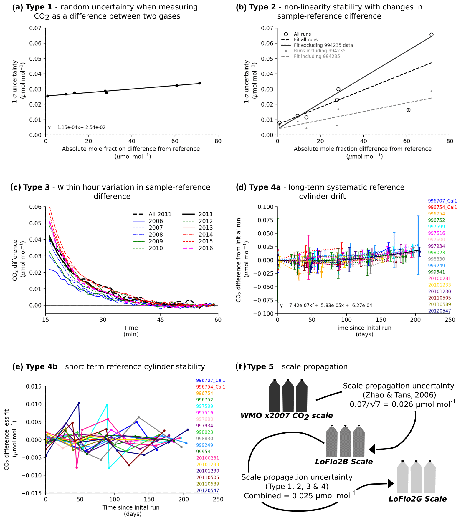
Figure 2 Error components of the Macquarie Island data site. (a) Mean of the mean SD of the 1 min mole fractions calculated for each run of each calibration cylinder as determined using the non-linearity correction of the previous run (filled circles) and a linear fit to these data (solid line). (b) Mean SD of the difference between calibration cylinder mole fractions determined for each individual run and the mean cylinder mole fraction of all runs (open circles) and of runs that included cylinder 994 235 (closed circles). A linear fit to all runs (dashed black line), a linear fit to runs that included cylinder 994 235 (dashed grey line) and a linear fit to the all runs data excluding the 994 235 data point (solid black line) are also shown. (c) Mean minute CO₂ mole fraction difference from the mixing ratio averaged over minutes 55–59, for 6337 available hours in 2011 with 44 min of sampling (black, dashed) and for hours with CO₂ SD less than 0.15 µmol mol⁻¹ for all 44 min in the hour for each year as listed in the key. (d) Long-term drift in reference cylinder mole fraction over time for each reference cylinder as referenced in the key. (e) Short-term variability in reference cylinder mole fraction over time determined as the difference between the individual drift values of each cylinder and a quadratic fit to these values for each reference cylinder as listed in the key. (f) Scale propagation chain and an estimate of the associated scale propagation error for each step.

Like the reference gas cylinders, calibration cylinders are made using dry Southern Ocean air collected at Cape Schanck, which is then modified to achieve targeted mole fractions higher or lower than ambient using aliquots of pure CO₂ or CO₂-free air (air which has had the CO₂ chemically stripped during collection). The concentrations of these MQA calibration cylinders are made using the Aspendale LoFlo (LoFlo 2B) following an identical procedure to that described above. The concentrations of the LoFlo 2B suite have been provided by the World Meteorological Organisation (WMO) Central Calibration Laboratory (CCL) made using conventional NDIR relative to the WMO X2007 scale (Zhao and Tans, 2006). This calibration propagation pathway is shown in Fig. 2f. Mole fraction assignment through the LoFlo instrument (typical uncertainty < 0.01 µmol mol⁻¹, Francey et al., 2010, Supplement) has been shown to be more precise than that of conventional NDIR (0.07 µmol mol⁻¹, Zhao and Tans, 2006).

The LoFlo2B calibration suite was calibrated directly against the WMO X2007 scale by the CCL on two occasions, 8 years apart. Differences for individual cylinders varied, averaging 0.01 µmol mol⁻¹ over the 8-year period. As these differences do not vary consistently with time or concentration it is likely that these differences reflect random uncertainty in the CCL's measurement method rather than actual changes in CO₂ mole fraction. As such, CO₂ assignments used here are the mean values of the two CCL calibrations. A detailed uncertainty analysis of this calibration approach is given in Sect. 3.4.

Table 1 Calibration cylinder concentrations on the WMO X2007 scale as measured by LoFlo2B or GASLAB. Suite 2G-a was used from 2005 to April 2006 and Suite 2G-b from April 2006 to the present.

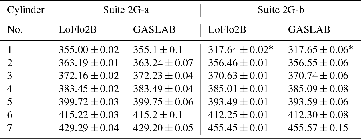
^* Only used April 2006 to March 2009.

Two CO₂ calibration suites, each containing seven 29.5 L high-pressure aluminium cylinders, have been used at Macquarie Island. The first suite, Suite 2G-a (Table 1), was installed with the system in 2005. However, this suite was accidentally partly vented and was replaced in April 2006 with a second calibration suite, Suite 2G-b (Table 1). In March 2009 use of the lowest CO₂ cylinder of Suite 2G-b was stopped, as its mole fraction (317.64 µmol mol⁻¹) was far lower than mole fractions observed at MQA. For comparison the two LoFlo2G suites (2G-a and 2G-b) and reference cylinders were also measured using gas chromatography (Francey et al., 2003), giving very similar mole fraction to those determined using LoFlo2B (Table 1).

3.4 Uncertainty analysis

Measurement uncertainty is typically composed of multiple elements and evaluated using a statistical analysis of replicate measurements (Type A) or based on an alternate source of information (Type B) (Klausen et al., 2016). The individual Type A and Type B components are then combined, usually in quadrature, to determine the overall measurement uncertainty. An example of this model can be found in Andrews et al. (2014), who evaluate, in detail, the uncertainty associated with tall-tower GHG measurements.

It is particularly important to characterise the measurement uncertainty of the MQA record given the small atmospheric signals at midlatitudes to high latitudes in the Southern Hemisphere. An earlier study documents the significant impact of measurement errors and biases of LoFlo, conventional NDIR and flask measurements on CO₂ growth rate estimation at Cape Grim, another key Southern Hemisphere site (Francey et al., 2010).

Here, following the approach discussed earlier, we aim to quantify the measurement uncertainty of the MQA CO₂ observations by examining each of five possible sources of error. We will examine how these errors contribute to the uncertainty of hourly and minutely mean values and combine them to determine estimates of the overall measurement uncertainty.

MQA measurements were calibrated following a multi-stage protocol (Fig. 2f), which uses a shallow quadratic non-linearity correction, based on the difference between the reference and sample raw instrumental response and the fixed mole fractions of the calibration standards (Sect. 3.3). Key sources of uncertainty in this approach are as follows:

1. The random uncertainty in measuring the CO₂ difference between two gases (Type 1),

2. the accuracy of the non-linearity correction with changes in the absolute mole fraction difference between the reference and sample at both the minutely and weekly timescale (Type 2),

3. systematic within-hour variation in the sample-reference CO₂ difference during the 50 min sample measurement period (Type 3),

4. the mole fraction stability of the reference standard over time (Type 4),

5. the propagation of mole fractions to the 2G calibration suites from the WMO X2007 scale via the LoFlo2B instrument (Type 5).

Here we quantify each of these five contributions to measurement uncertainty, thus providing a framework for defining uncertainties specific to data applications, e.g. involving different averaging periods or comparison with other data sets. Combining uncertainties of all five types in quadrature defines the overall measurement uncertainty when comparing measurements, including those of other laboratories, that are independently calibrated against the WMO X2007 scale. Comparisons of measurements made within the CSIRO network on similar instruments relative to LoFlo2B will have a significantly smaller Type 5 component. The uncertainty analysis uses only data with stable instrumental temperature and pressure and also excludes measurements made shortly after valve switches to minimise line conditioning effects. Uncertainties inherent in the sample handling or intake system, involving potential modification of sample air before being admitted to the LoFlo instrument, have not been examined.

3.4.1 Type 1 and Type 2 uncertainty: the random uncertainty in measuring the CO₂ difference between two gases and the accuracy of the non-linearity correction with changes in the absolute mole fraction difference between reference and sample

These two uncertainty types were assessed using regular measurements of the second suite of calibration standards (2G-b) as a proxy for in situ air data. This analysis was based on 80 calibration runs between 2006 and 2013. Each calibration run included between 16 and 144 (mean = 84) min of retained raw data for each individual calibration standard.

Minute-mean mole fractions of the calibration standard data (i.e. the proxy air samples) were calculated for each run using the non-linearity correction determined in the previous calibration run. This represents a worst-case scenario, as in situ mole fractions will generally be calculated using a non-linearity correction determined much closer in time and will not be affected by any regulator or gas handling or switching effects.

First we examined uncertainty in the non-linearity correction characteristic of the 1 min timescale. The minute-mean 1σ uncertainties of these proxy air samples were determined, for each calibration standard, as the mean 1 min standard deviation (SD) for each run averaged over the 80 calibration runs. These 1σ uncertainties were compared to the absolute mole fraction difference between calibration and reference standards (Fig. 2a). This shows a clear mole fraction dependence, with the 1σ uncertainty for a minute-mean increasing from 0.025 µmol mol⁻¹, at close to the reference mixing ratio (this is the Type 1 random uncertainty component inherent in measuring the CO₂ difference between two cases due to instrument precision and counting time), to 0.034 µmol mol⁻¹ when the absolute sample reference mole fraction difference was 70 µmol mol⁻¹.

The slope of the line is 0.0001, indicating an uncertainty of 0.01 % of the sample-reference mole fraction difference at a 1 min timescale. This Type 2 mole fraction dependent component of uncertainty is negligible for the vast majority of in situ measurements since at MQA, 99.9 % of minute measurements are within 10 µmol mol⁻¹ of the reference standard.

The same data set was used to evaluate uncertainty in the non-linearity correction over timescales of a few weeks, which relates to the time period between calibration runs. For this case we calculated the mean CO₂ mole fraction per calibration standard per run, still using the non-linearity corrections defined by the previous calibration runs made typically 4 to 6 weeks prior. Variability in the mean from run to run (as expressed by the SD of residuals of these means from the mean of all runs) was plotted against the absolute difference from the reference standard mole fraction (Fig. 2b open circles, a linear fit to the data is shown as the dashed black line). Retained data included 18 runs for standard 994 235 and 37 runs for the other six standards. As such, 18 of the non-linearity corrections included in this analysis were based on 7 calibration cylinders while the remaining 37 used only 6 cylinders. In this analysis it was assumed that the calibration standard mole fractions were stable, and hence any mole fraction variability was due to changes in the instrumental response.

Standard 994 235 was a clear outlier in this analysis (low open circle Fig. 2b). This was the standard dropped from analysis in March 2009 (Sect. 3.3) and is possibly attributable to a shorter analysis period: less than three years compared to greater than six years for the other six standards. To investigate this further the analysis was repeated using only runs that included 994 235 (18 runs of all seven cylinders, Fig. 2b small closed circles) and a linear fit to those data (panel a). A linear fit (panel b) to the data from all runs but excluding the standard 994 235 data point was also calculated (Fig. 2b black solid line). The slope for panel (a) is shallower than that for panel (b), 0.0003 compared with 0.0008, indicating less uncertainty in mole fractions assigned using calibration runs which included cylinder 994 235. This may be due to the tighter constraint on the quadratic fit (i.e. using seven rather than six calibration cylinders) or possibly a deterioration in instrumental stability over time. There is also evidence of higher variability in instrument non-linearity over longer timescales (weeks vs. minutes), with an 8-fold larger uncertainty found for the ∼ monthly (Fig. 2b slope 0.0008) compared to the minutely (Fig. 2a slope 0.0001) time frame.

Interestingly the y intercept shows the run-to-run random uncertainty for repeat cylinder measurements as 0.004 µmol mol⁻¹. This is independent of the inclusion of cylinder 994 235 but is slightly larger than the random uncertainty determined when scaling the minute-mean Type 1 uncertainty using the root mean square to a matching run length (i.e. $\mathrm{0.025}/\sqrt{\mathrm{84}}=\mathrm{0.0027}$ µmol mol⁻¹ where 84 is the average number of minutes in a calibration run). This is probably driven by drifts in the calibration cylinder mole fractions over time.

As for the Type 2 uncertainty in minute means, this component is again typically very small, less than 0.008 µmol mol⁻¹ for sample-reference differences of less than 10 µmol mol⁻¹.

3.4.2 Type 3 uncertainty: within-hour variation in the sample-reference CO₂ difference

Between calibration runs, which are performed several weeks apart, the instrument operates in routine in situ monitoring mode. This involves an hourly cycle of alternating measurements of reference and ambient MQA air. The first 10 min of each hour are used for reference measurements (reference in both cells) to determine the difference in output between cells. This difference is used by the data-processing algorithm to define a background signal, interpolated between successive reference measurements made every hour, against which ambient CO₂ measurements are subsequently quantified. Ambient air is then admitted to the sample side cell and measured relative to the reference (in the reference side cell) for the remaining 50 min of the hour.

The first 6 min of data from both the reference and ambient air measurement periods are excluded from further processing due to stabilisation of flow rate and pressure in the sample side cell after the valve switch. For ambient air, CO₂ measurements are obtained for the remaining 44 min of the hour. However, further investigation into the stability of these data has revealed subtle, systematic drifts in minute-mean CO₂ over the 44 min period.

In order to resolve these small instrumental artefacts in ambient CO₂ data, we consider only hours with small atmospheric CO₂ variability. Figure 2c shows minute-mean mole fraction deviations from the average of the last 5 min in each hour, averaged by calendar year and over hours that (i) contain the complete 44 min of retained data and (ii) have a minute-mean SD of CO₂ < 0.15 µmol mol⁻¹. For comparison purposes, data are also presented for a single year (2011) with no selection for low CO₂ variability. This curve is slightly noisier, however the magnitude and time dependence of CO₂ deviations is similar to the case with data selection.

The curves for different years are very similar in shape, with deviations being largest in the early minutes and then decaying to zero at around minute 45. There is a suggestion that the magnitude of deviation has increased over time, with 2006 showing the smallest deviation at minute 16 of 0.02 µmol mol⁻¹ and 2014 the largest of 0.06 µmol mol⁻¹. The cause of this within-hour drift has not been confirmed, but is suspected to result from re-equilibration of the internal surfaces of the Nafion drier (Naudy et al., 2014) to disruption of sample air flow during the 10 min reference measurement period.

We assume here that the latter, more stable part of the ambient measurement period provides the most reliable CO₂ measurements and thus we construct our hourly data set using the mean of 30 min of data collected between minutes 30–59 of each hour, with a timestamp of 45 min past the hour. This is a compromise between maximising the number of minutes contributing to hourly means and limiting any systematic bias associated with the time-dependent drift. The bias in hourly means calculated this way, relative to the last 5 min of the hour, is within 0.003 µmol mol⁻¹. We take this figure to represent the uncertainty characteristic of the within-hour (Type 3) drift that is applicable to the comparison of hourly means.

Definition of the Type 3 uncertainty applicable to minute means is more complex, as it comprises both random and systematic components, varies with minute number within the hour, and in some respects, increases with time (i.e. increasing maximum deviation between 2006 and 2014 as displayed in Fig. 2c). For the purpose of quantifying the random component in a way that can be simply integrated with the overall uncertainty analysis presented here, we conducted a second analysis calculating the variability in minute-mean deviation from the mean of minutes 55–59 across all low CO₂ variability hours in 2011. This indicates that variability is largest at minute 16 and diminishes to zero by the latter part of the hour, which is consistent with the earlier description of the magnitude of the artefact. We use the minute 16 figure of 0.02 µmol mol⁻¹ as a representative estimate of the random uncertainty component. We do not include the systematic uncertainty in subsequent calculations but note that (i) this should be considered in any comparisons of minute-mean data and (ii) there is potential to correct for this artefact, for example using the averaged annual behaviour from Fig. 2c.

3.4.3 Type 4 uncertainty: stability of the reference cylinders over time

The uncertainty inherent in assuming that the CO₂ mole fraction of the reference standard (reference mole fraction) is constant over time was investigated by calculating the change in assigned reference mixing ratio. This was determined as the difference between the first and subsequent calibration runs for each of the 18 reference standards. Although the number of calibration runs varied for each standard, all were analysed at least 3 times (average of 5.7) over a period of 40 to 202 (average of 158) days (Fig. 2d). The mean systematic drift was determined from a quadratic fit to the difference data (black line Fig. 2d), indicating a drift of 0.0017 µmol mol⁻¹ averaged over a month (the average time between calibration runs).

The short-term variability of each cylinder (Fig. 2e) was separated from the systematic drift by fitting and then subtracting a quadratic (representing long-term drift) from each standard's set of differences. The SD of short-term variability values for each standard was determined and the average of all cylinders was calculated to give a mean 1σ uncertainty of 0.0021 µmol mol⁻¹. Combining the short-term variability and systematic drift results in an overall Type 4 uncertainty of 0.0038 µmol mol⁻¹ in the stability of the reference standard mole fraction.

3.4.4 Type 5 uncertainty: propagation of the WMO X2007 scale to the 2G calibration suite

The mole fractions of the 2G calibration suite were linked to the WMO X2007 scale using measurements made on LoFlo2B against the 2B calibration suite, which is, in turn, linked to the WMO X2007 scale (Fig. 2f). Hence the propagation uncertainty for the 2G calibration suite will consist of both the propagation uncertainty between it and the primary WMO X2007 scale (via the 2B calibration suite) and the uncertainty inherent in 2B measurements. Zhao and Tans (2006) give the random uncertainty associated with propagation of the NOAA primary scale to individual standards as 0.07 µmol mol⁻¹. As such, the propagation uncertainty for the 7-cylinder LoFlo2B suite will be 0.026 (i.e. $\mathrm{0.07}/\sqrt{\mathrm{7}}$) µmol mol⁻¹.

Similarly to the earlier discussion for LoFlo2G, the remaining LoFlo2B uncertainties can be separated into Types 1, 2, 3 and 4. Combining in quadrature the 2B propagation uncertainty with Type 1, 2, 3 and 4 uncertainties estimated based on the worst-case 2G uncertainties, the 2G WMO X2007 propagation error was estimated as 0.024 µmol mol⁻¹. This estimate is based on an average run length of 84 min of raw data and mean reference-to-sample mole fraction difference of 30 µmol mol⁻¹. This is expected to be an overestimate of the instrumental uncertainties in the 2B data due to the vastly differing laboratory environments and hence conditions of the two instruments. LoFlo2G was developed in the same laboratory as LoFlo2B but has since been transported by sea to Macquarie Island, had only limited maintenance (Sect. 2) and measured predominantly wet, salty ambient air.

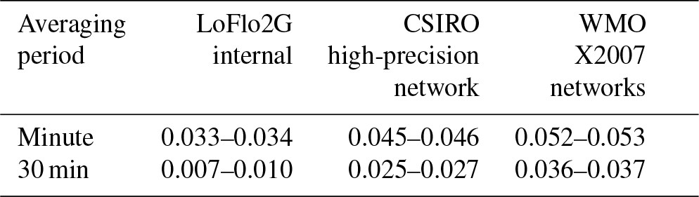
Table 2 Combined uncertainty estimates in µmol mol⁻¹ applicable to comparisons with different data sets for minute-mean data and hourly data based on averaging the final 30 min of each hour. The uncertainty estimates are given as a range spanning sample to reference differences of 0–10 µmol mol⁻¹.

3.4.5 Overall uncertainty

By geometrically combining appropriate uncertainty types and selecting key factors, it is possible to give a series of examples of the expected minute-mean and hourly uncertainties for different situations (Table 2). These examples all use the worst-case Type 3 and 4 uncertainty estimates.

Typically the uncertainty is dominated by the Type 5 uncertainty component, which in turn is comprised mainly of the propagation uncertainty to the WMO X2007 scale. As such, the applicable uncertainty is highly dependent on the network choice, decreasing by up to 40 % when considering within-network CO₂ comparisons for CSIRO high-precision instruments referenced to the LoFlo2B calibration suite (e.g. the Cape Grim and MQA LoFlos) compared to between-network comparisons calibrated to the WMO X2007 scale. For a 30 min mean observation with a mole fraction near the reference cylinder mole fraction (>99.9 % of MQA observations), these uncertainties would be 0.025 and 0.036 µmol mol⁻¹ for within- and between-network comparisons respectively. In comparison, the increase with sample to reference difference is typically much smaller, for example a 0.003 µmol mol⁻¹ increase in uncertainty for a 20 µmol mol⁻¹ increase in the sample to reference difference of a 30 min mean.

Figure 3 Minute mean (black dot, left axis) and SD (blue dot, right axis) of CO₂ mole fraction for days 230–260 (18 August to 17 September) in 2011. Red dots and bars on day 230 and day 249 are CO₂ mole fraction and 1σ uncertainty from flask samples.

4 Data characteristics and comparison with flask measurements

4.1 Typical features of the CO₂ record

MQA CO₂ data display a number of characteristics which we illustrate here by showing a 30-day subset (18 August–17 September 2011) of minute-mean and SD of CO₂ mole fractions (Fig. 3). The minute means and SDs are calculated from the raw 2 Hz data. The period was chosen because it has good data coverage of both CO₂ and wind data and radon was being measured through this period, although with poor data quality as noted in Sect. 2.

The minute-mean CO₂ mole fractions, shown in Fig. 3, are around 389 µmol mol⁻¹, increasing slightly over the 30 days. For most of the period, mole fractions within an hour vary by 0.1–0.3 µmol mol⁻¹, while variations over a day are typically 0.5–1.0 µmol mol⁻¹. There are also larger positive and negative deviations of 2–3 µmol mol⁻¹. The positive deviations (e.g. day 238, day 242 and day 256) are characterised by elevated SD, while the negative deviations are not (e.g. day 235, day 247). During this period, flask samples were filled on 18 August (day 230) and 6 September (day 249). The flask mole fractions on day 230 agree reasonably well with the in situ measurements. By contrast, the flasks filled on day 249 do not have good flask pair agreement, with the higher mole fraction flask being around 1.7 µmol mol⁻¹ above the coincident in situ measurement. It is worth noting that this flask had already been flagged as an outlier by the standard flask-fitting and quality checks applied to the flask record. Flask and in situ measurements are compared across the full in situ record in Sect. 4.3.

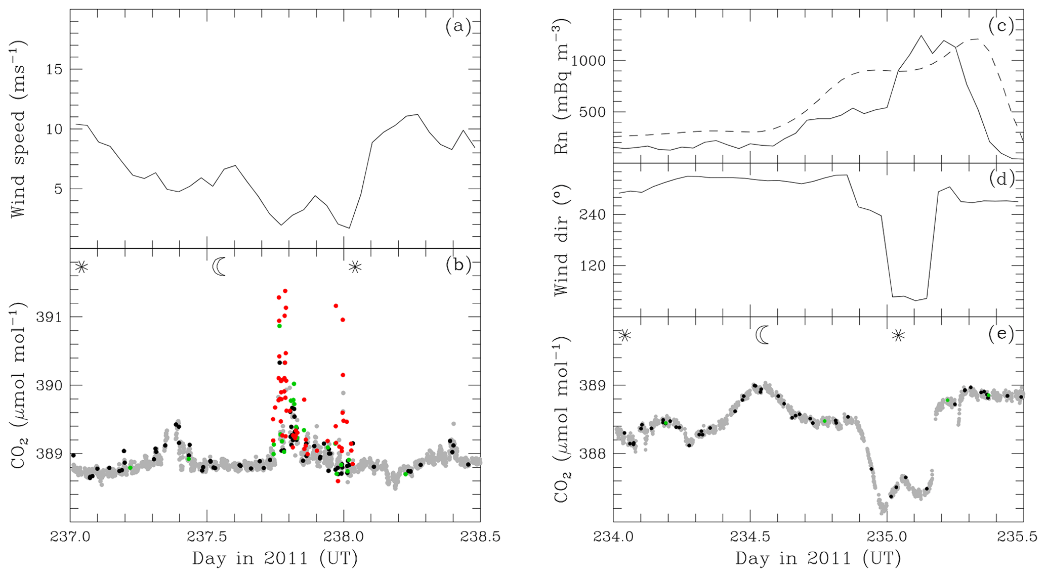
Figure 4 Hourly wind speed (a) and minute-mean CO₂ mixing ratio (b) for days 237–238.5 (25 August 00:00 UT to 26 August 12:00 UT) in 2011. Hourly observed (solid) and modelled (dashed) radon concentration in mBq m⁻³ (c), wind direction (d) and minute-mean CO₂ mole fraction (e) for days 234–235.5 (22 August 00:00 UT to 23 August 12:00 UT) in 2011. CO₂ mixing ratio is coloured according to CO₂ SD: less than 0.10 µmol mol⁻¹ (grey), 0.10–0.12 µmol mol⁻¹ (black), 0.12–0.15 µmol mol⁻¹ (green) and greater than 0.15 µmol mol⁻¹ (red).

Figure 4 provides a closer look at one positive deviation and one negative deviation. The increased mole fractions around day 237.8 to 238.0 (Fig. 4b) are at times of lower wind speed (Fig. 4a), indicative of a local influence on observed CO₂ mole fractions. In general, as with this example, deviations associated with low wind speed are more often positive than negative, suggesting a contribution from anthropogenic sources as well as biospheric sources and sinks. The categorisation of the minute means by SD (indicated by the dot colour in Fig. 4) shows that large deviations are mostly, but not always, associated with high SD. This is important to note when considering whether CO₂ SD is helpful for data selection (Sect. 5).

Figure 4e focuses on a negative CO₂ deviation around day 235. This deviation is coincident with a change in wind direction from westerly to north-easterly (Fig. 4d) and increased radon concentrations (Fig. 4c), both modelled (see Sect. 5.2) and observed. The modelled radon shows a somewhat broader peak than observed but captures the main features of the event. The wind speed through this period (not shown) was greater than 10 m s⁻¹. Elevated radon is a good marker of air that has had significant contact with land surfaces over the previous week or so. Consequently, the negative deviation in CO₂ mole fraction is likely due to biospheric uptake of CO₂. Back trajectories (not shown) suggest the uptake occurred over Tasmania and southern Australia, before the air mass was transported to Macquarie Island. CO₂ SDs are low throughout this period, with only occasional minutes in the 0.10–0.15 µmol mol⁻¹ range and most of those less than 0.12 µmol mol⁻¹.

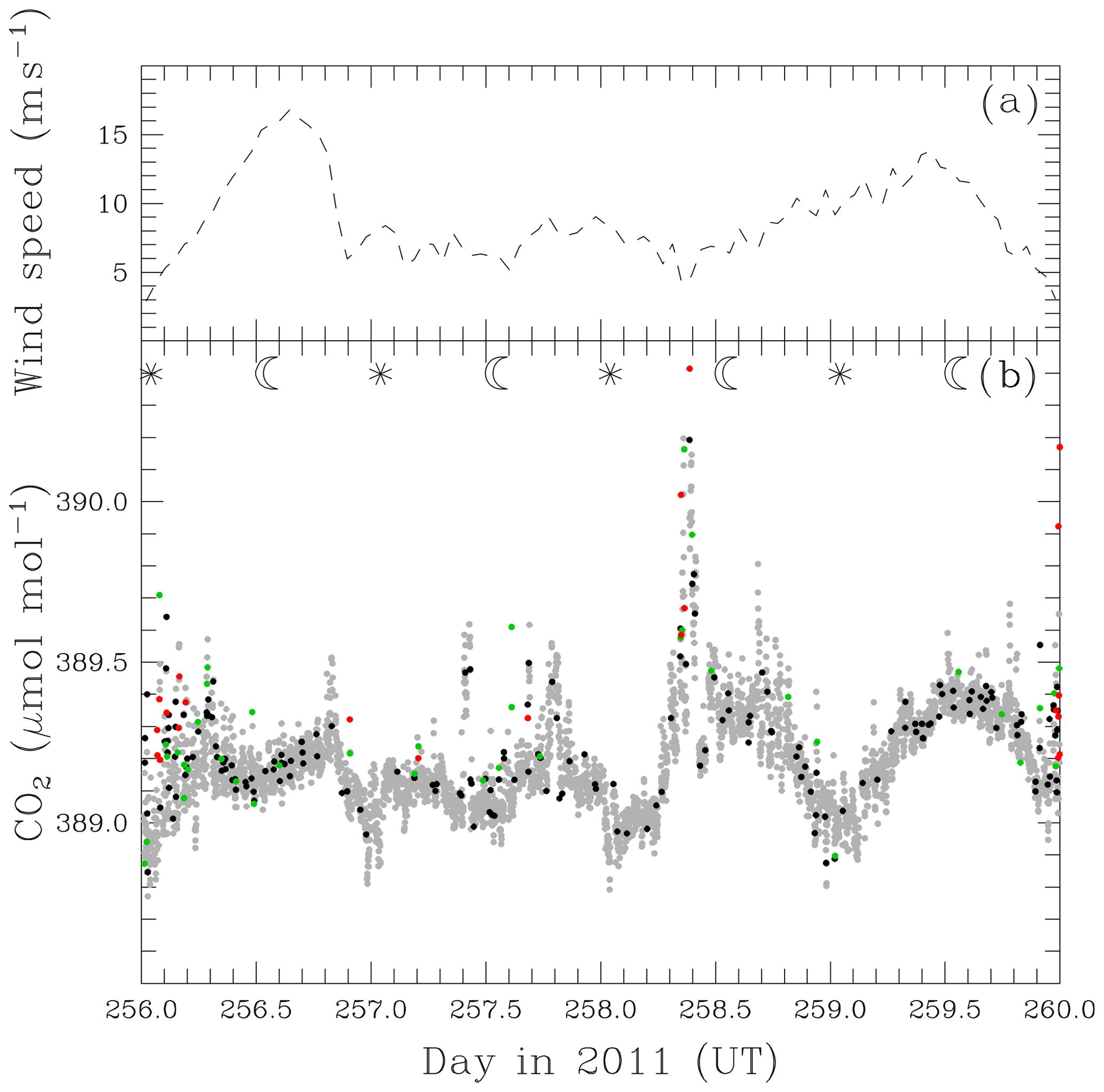
Figure 5 Hourly wind speed (a) and minute-mean CO₂ mixing ratio (b) for days 256–260 (13 September 00:00 UT to 17 September 00:00 UT) in 2011. CO₂ mole fraction is coloured according to CO₂ SD: less than 0.10 µmol mol⁻¹ (grey), 0.10–0.12 µmol mol⁻¹ (black), 0.12–0.15 µmol mol⁻¹ (green), greater than 0.15 µmol mol⁻¹ (red).

Finally we examine a period without large deviations (Fig. 5). This period shows some sensitivity to wind speed, with higher CO₂ SD and more scatter in the minute-mean CO₂ when the wind speeds are lower (e.g. around the start of day 256). Also apparent here is a diurnal cycle, with lower CO₂ values around 00:00–02:00 UT (11:00–13:00 LT). This is more evident in the last 2 days shown (peak-to-trough amplitude of ∼ 0.5 µmol mol⁻¹), than the first 2 days.

In the remainder of this section and in Sect. 5, we further explore each of the features identified here, examining how widespread they are across the whole record and the implications for selection of the data record for different purposes.

Figure 6 Frequency histograms of (a) the SD of CO₂ mole fraction within a minute for all available minutes in 2011 for Macquarie Island (solid) and Cape Grim (dashed) and (b) the nearest hourly wind speed to all available minutes in 2011 with CO₂ SD less than 0.10 µmol mol⁻¹ (solid), 0.10–0.12 µmol mol⁻¹ (long dash), 0.12–0.15 µmol mol⁻¹ (short dash) and greater than 0.15 µmol mol⁻¹ (dotted).

4.2 CO₂ standard deviation and wind speed

The distribution of minute SDs of CO₂ mole fraction for all available data in 2011 is shown in Fig. 6a; other years were similar. The distribution has a mean of 0.076 µmol mol⁻¹ with a slightly smaller mode (peak), 0.060–0.065 µmol mol⁻¹. The distribution has a long upper tail, with 1.26 % of values between 0.20 and 0.40 µmol mol⁻¹, and 0.38 % above 0.40 µmol mol⁻¹ (up to the maximum SD of 2.20 µmol mol⁻¹). The MQA distribution is compared with the corresponding distribution for 2011 measurements at Cape Grim, Tasmania (144.7^∘ E, 40.7^∘ S), made using a similar instrument. Cape Grim SDs were generally smaller than for MQA, with a mean of 0.063 µmol mol⁻¹ and mode of 0.040–0.045 µmol mol⁻¹. The difference is most likely due to the sampling height and inlet length at the two sites. Cape Grim air is sampled at 70 m from a tower that is on the top of an approximately 100 m high cliff. By contrast, Macquarie Island air is sampled from 7 m (13 m a.s.l.).

Figures 4 and 5 suggested a relationship between CO₂ SD and wind speed. This can be seen more clearly in Fig. 6b, which shows the distribution of the nearest hourly wind speed to each available minute in 2011 for different CO₂ SD ranges. For SDs less than 0.10 µmol mol⁻¹ (almost 90 % of all data), the distribution is broad with a peak around 13 m s⁻¹. The distribution for the 0.10–0.12 µmol mol⁻¹ SD range is similar, with a small increase in the proportion of minutes with wind speeds less than 7 m s⁻¹. By contrast the distributions for larger SDs are shifted to lower wind speeds, with the peaks of the distribution around 5 and 3 m s⁻¹, respectively, for SDs between 0.12–0.15 µmol mol⁻¹ and greater than 0.15 µmol mol⁻¹. For the largest SD category, 87 % of the distribution is below 8 m s⁻¹. This confirms the hypothesis from the example case above, that CO₂ measurements are noisier at lower wind speeds, indicative of an influence from local CO₂ fluxes and likely exacerbated by the relatively low sampling height. Figure 6b also provides evidence that CO₂ minute SDs may provide a good alternative to wind speed as a criterion for removing local influences from the CO₂ record.

4.3 Comparison of flask and in situ measurements

Since 1992, pairs of air samples have been collected fortnightly at MQA, in 0.5 L glass flasks using flask sampling techniques described by Francey et al. (1996). From 1992 to 1995 these flasks were sealed with polytetrafluoroethylene (PTFE) O-rings, but since 1996 perfluoroalkoxy (PFA) O-rings were used. Flask sampling is performed when wind speeds are > 7 m s⁻¹ and the wind direction is from the north-west (290–360^∘) or south-east (110–180^∘) quadrants, to avoid local biogenic and anthropogenic sources and sinks (Fig. 1). Although mounted on the same mast as the LoFlo intake line, the flask sampling intake line, along with its drying and pump systems, are entirely separate to that of the LoFlo.

Filled flasks are stored and then shipped back annually to CSIRO GASLAB (Aspendale, Australia), where they are analysed for CO₂ and its isotopes δ¹³C and δ¹⁸O, CH₄, H₂, CO and N₂O (Francey et al., 2003). Data are flagged if the sampled air mass was not representative of baseline conditions, if they were affected by sampling or analytical artefacts, or if they lie more than three SDs from the smoothed-curve fit to the atmospheric record using the methods of Thoning et al. (1989). Flagged data were not used for this analysis.

All measurements derived from CSIRO flask samples require a correction for the loss of CO₂ with storage time due to permeation of gases through the O-rings (Langenfelds et al., 2002; Sturm et al., 2004).

Figure 7 Storage time (a) in days, storage correction (b) in µmol mol⁻¹ for flasks filled at Macquarie and the mole fraction difference (c) between the flask mole fraction and the mean Loflo2 mole fraction for the two 30 min averages that span the flask (or if both not available, the single 30 min average within 1 h of the flask fill time). Mole fraction differences are shown for all flasks that had a flask pair difference less than 0.4 µmol mol⁻¹ (+), for all flasks that had a flask pair difference greater than 0.4 µmol mol⁻¹ (o) and for flasks without a pair (x). Flagged flasks are not used.

These corrections are especially significant for CSIRO's low-volume (0.5 L) flasks and at sites such as MQA, where storage times can exceed a year. Loss rates have been determined by comparing data from CSIRO's southern high-latitude sites, where flasks can be stored for a year or so before analysis, with smoothed baseline concentrations at Cape Grim, Tasmania, derived from flask sample data with relatively short storage times. Using data from 1992 to 2007, a correction of 0.002 $\mathrm{\mu }\mathrm{mol}{\mathrm{mol}}^{-\mathrm{1}}{\mathrm{day}}^{-\mathrm{1}}$ was estimated for flasks fitted with PFA O-rings and filled to 85 kPa above ambient pressure (Langenfelds et al., 2011), leading to storage corrections of up to 1 µmol mol⁻¹ for MQA flask samples (Fig. 7a, b).

LoFlo observations were compared to individual flask sample data by taking the mean of the hours before and after the flask filling time or either hour if only one was available. This identified 361 matching records after flagged flasks had been excluded. Flask-LoFlo concentration differences are shown in Fig. 7c, with differences ranging from −1.3 to 0.9 µmol mol⁻¹. Flasks are filled in pairs to help assess measurement quality with the expectation that the two flasks will give similar CO₂ measurements, ideally within 0.1 µmol mol⁻¹. Figure 7c shows that when flask pair differences are larger (greater than 0.4 µmol mol⁻¹), one of the pair often has an outlying flask-LoFlo difference, suggesting a less reliable flask measurement. The mean flask-LoFlo mole fraction difference is −0.13 µmol mol⁻¹, with an SD of 0.27 µmol mol⁻¹. The limitations of the flask record compared to that of the LoFlo instrument are further explored in Sect. 6 when defining a CO₂ climatology for Macquarie Island.

5 Defining a baseline record

The aim of most long-term atmospheric CO₂ measuring sites is to provide regional baseline CO₂ observations. Thus, most sites employ some site-specific criteria to select those observations that are considered to be independent of local and point sources and sinks. For coastal sites, it is usual to try to select oceanic air with no recent land contact. For flask samples, this selection is largely independent of measurement and often based on some specified meteorological conditions such as wind speed and direction. For in situ measurements, selection is a post-measurement process, opening a range of possibilities for different data selection for different purposes. Methods of data selection include meteorological (usually wind) criteria, the concentration of other key atmospheric components (e.g. Rn, Chambers et al., 2016), back trajectories, air mass origin maps, various statistical methods (e.g. El Yazidi et al., 2018) and, due to the high temporal frequency of the measurements, removal of outliers using a statistical fitting procedure (e.g. Thoning et al., 1989). The remoteness of Macquarie Island makes defining the baseline record simpler than for many other sites. The aim is, firstly, to remove measurements that are influenced by any local fluxes from the island itself (likely to be small as the land fetch from the predominant wind directions is <100 m) and, secondly, depending on the application, to remove air samples that have had relatively recent contact with other Southern Hemisphere land (for example Fig. 4e). The selection is applied to the hourly measurement record, noting that hourly reported mole fractions are actually 30 min averages, as described in Sect. 3.4.2.

5.1 Removing local flux influences

Local flux influences on the CO₂ record are often removed using a wind speed criterion. Given the relationship described in Sect. 4.2 between CO₂ SD and wind speed, we explore the effectiveness of CO₂ SD as a baseline selection method. An obvious advantage of this approach is that it is not dependent on a separate meteorological data set that may have measurement gaps. A number of CO₂ SD measures could be used for this purpose. Based on the behaviour seen in Fig. 4b, we reject a 30 min average measurement based on the magnitude of the noisiest minute contributing to that average. Figure 4b showed that most but not all outlier minute CO₂ mole fractions have high minute CO₂ SD. Using the maximum minute SD (MMSD) across the averaging period helps to ensure that any outliers with low CO₂ SD are also excluded. We also exclude any 30 min average which had missing minutes within the averaging period.

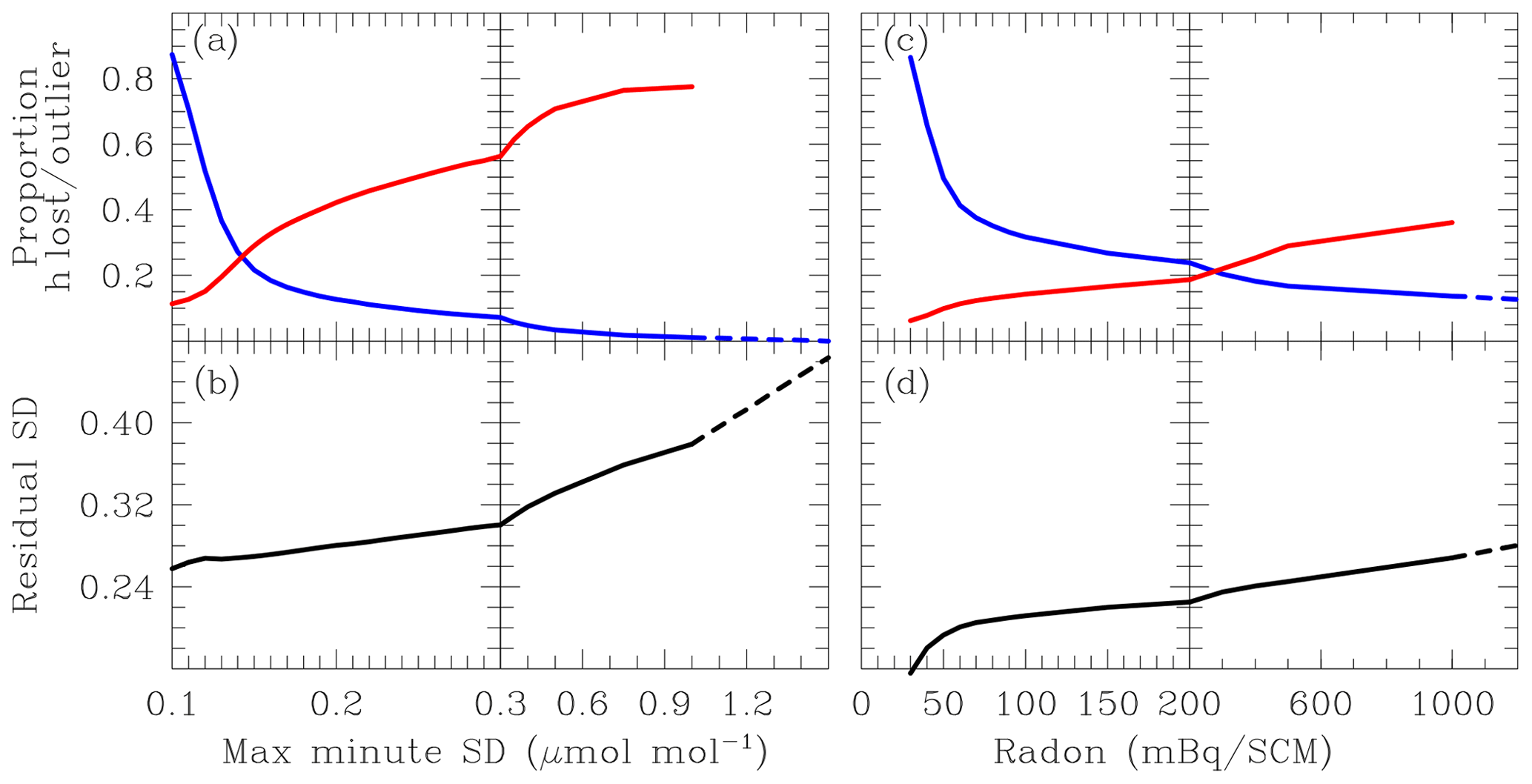
Figure 8 Proportion of hours lost (blue) and proportion of rejected hours that are outliers (red) for a given minute CO₂ SD rejection criteria (a) and for a given radon rejection criteria in addition to maximum minute CO₂ SD selection of 0.2 µmol mol⁻¹ (c). Outliers are defined as hours with a mole fraction residual from a smooth curve fit greater than 0.5 µmol mol⁻¹. Standard deviation of residuals from a smooth curve fitted to data selected by the maximum minute CO₂ SD (b) and selected by radon concentration in addition to maximum minute CO₂ SD of 0.2 µmol mol⁻¹ (d).

We test this selection technique by rejecting data for a range of MMSD values. Effective selection is demonstrated by a reduction in short-term variability in the data through removal of outliers without excessive data rejection. The short-term variability is determined by fitting a smooth curve to the hourly data (Sect. 5.3), subtracting this from the hourly data to give a time series of residuals and then calculating the SD of the residuals. Figure 8 shows that, as the MMSD rejection value is reduced, the residual SD initially decreases rapidly (Fig. 8b), while the proportion of hourly data rejected increases relatively slowly (blue curve, Fig. 8a). At 0.3 µmol mol⁻¹ only about 7 % of hours are rejected but the residual SD has been reduced by 35 % (from 0.46 to 0.30 µmol mol⁻¹). As the rejection value is reduced further, the residual SD continues to decrease, but below about 0.15 µmol mol⁻¹ the data loss starts to increase more rapidly.

Figure 9 CO₂ mole fraction (µmol mol⁻¹) at hourly frequency (a, b) and fitted with a smooth curve (c). Hourly frequency data are 30 min means where the 30 min means have been selected only for no missing minutes (black, a), additionally for maximum minute CO₂ SD less than 0.2 µmol mol⁻¹ (red, a, b) and additionally for model-simulated radon concentration less than 60 mBq SCM⁻¹ (blue, b). (c) shows the curve fits for each of the three plotted data sets (solid, colours as a, b) and the difference in the curve fit (right axis) from the radon-selected fit for missing data-only selection (dotted, black) and for maximum minute CO₂ SD selection (dotted, red).

Figure 8a also shows the proportion of rejected data that are outliers (defined as the magnitude of a residual being greater than 0.5 µmol mol⁻¹). As the MMSD rejection value is reduced the proportion of outliers rejected becomes smaller; by 0.25 µmol mol⁻¹ the selection is removing as many low residual data points as outliers (red curve, Fig. 8a). The analysis suggests that a MMSD rejection value between 0.15 and 0.20 µmol mol⁻¹ provides the best compromise between minimising residual spread and maximising data retention. Figure 9a shows average hourly mole fraction from 2006 to 2017 selected using a MMSD rejection value of 0.20 µmol mol⁻¹ compared to all hourly values (selected only for no missing minutes). The selection tends to remove positive outliers throughout the year and some negative outliers in summer. This would be consistent with the removal being mostly of measurements influenced by local anthropogenic fluxes with a smaller influence from the biosphere on Macquarie Island.

5.2 Removing Southern Hemisphere land flux influences

Figure 4c, e demonstrates that elevated radon concentrations are a good indicator of air samples that have been influenced by long-range transport from Southern Hemisphere continents. Radon observations are not available for the whole period of MQA LoFlo CO₂ measurements. Consequently, to ensure that the CO₂ record (2005–2016) is treated consistently, we test the feasibility of using model-simulated radon concentrations for data selection. Where the observed and modelled records overlap, the modelled radon is broadly consistent with the observations but with generally lower baseline concentrations. This means that the analysis presented here, to choose an appropriate radon selection threshold, is applicable to this modelled radon data set only and would need to be repeated if using the available observations or an alternative modelled radon data set.

Atmospheric radon concentrations are simulated as in Loh et al. (2015), except that the CSIRO Conformal-Cubic Atmospheric Model (McGregor, 2005; McGregor and Dix, 2008) is nudged to ECMWF winds (Dee et al., 2011) rather than the NCEP forcing used previously. Radon is input to the lowest model level at a constant rate of 21.0 $\mathrm{mBq}{\mathrm{m}}^{-\mathrm{2}}{\mathrm{s}}^{-\mathrm{1}}$ for land surfaces between 60^∘ S and 60^∘ N. Radon input is much lower for ocean surfaces and in polar regions. We use a flux of 0.11 $\mathrm{mBq}{\mathrm{m}}^{-\mathrm{2}}{\mathrm{s}}^{-\mathrm{1}}$ for all ocean surfaces between 70^∘ S and 70^∘ N and for land between 60 and 70^∘ in both hemispheres. We use zero flux poleward of 70^∘. Following injection, radon decays with a half-life of 3.8 days. Here we report hourly radon concentrations output from the model at the nearest grid cell to Macquarie Island (159.229^∘ E, 54.854^∘ S).

Figure 8c, d illustrates the effectiveness of different radon thresholds for removing data that may have been influenced by Southern Hemisphere land fluxes. The evaluation starts from the case shown in Fig. 9a, where local impacts have been removed using the MMSD criteria of 0.2 µmol mol⁻¹. Radon selection clearly reduces the residual SD (Fig. 8d) below that obtained from local selection alone. For example, the residual SD is reduced to 0.20 µmol mol⁻¹ for a radon threshold of 60 mBq SCM⁻¹. As with the local selection, there is a compromise between reducing residual SD and maintaining data quantity. The proportion of rejected data reaches 0.41 for a radon rejection value of 60 mBq SCM⁻¹ and increases rapidly as the radon rejection value is further reduced (Fig. 8c). Using the same outlier measure as in Sect. 5.1, only around a third or less of the additional data points rejected by radon selection are outliers. This may be because the model-simulated radon is likely to give a more diffuse signal than observations and hence would reject more data. It is also possible that air with a radon signal has traversed a continental region with little or no CO₂ flux and consequently is not seen as an outlier at Macquarie Island.

Figure 9b shows the impact of radon selection at 60 mBq SCM⁻¹ relative to MMSD selection at 0.2 µmol mol⁻¹. Both positive and negative outliers are removed, with negative outliers more prominent in spring.

5.3 Curve fitting

A smooth curve was fit to the hourly CO₂ data following the methods described in Thoning et al. (1989). The method allows us to decompose the time series into trend, seasonal cycle and residual components. The first step is to fit the data (using least squares) with a second-degree polynomial and four harmonics to represent the long-term increase in CO₂ and a mean seasonal cycle. While many applications of the Thoning et al. (1989) method iterate this fit, removing outliers after each iteration, this was not required for the MQA data set. Residuals from the polynomial plus harmonic fit were then filtered in the frequency domain, with transformation to the frequency domain using a sampling interval of 1 h. Two filters were applied to capture short- and long-term variations. An 80-day low-pass filter captures interannual variations in seasonality by retaining variability on weekly to monthly timescales. A 667 day low-pass filter captures interannual variations in CO₂ growth that are not represented by the second-degree polynomial. Either set of filtered residuals are combined with all or part of the polynomial plus harmonic fit to represent different features of the CO₂ time series.

Figure 9c shows the smooth curve fit to the hourly MQA CO₂ observations from combining the polynomial plus harmonic with the 80-day filtered residuals for the three data sets shown in Fig. 9a, b. The three cases are difficult to distinguish, confirming the relatively small number of outliers observed at Macquarie Island and their small influence on the fitted curve. Figure 9c also shows the difference in the fitted curves (right-hand axis) from the fit to the data set selected for both minute CO₂ SD and radon. Differences are mostly positive and up to 0.18 µmol mol⁻¹ for the fit to the data set selected only for no missing minutes, consistent with this data set having mostly positive outliers. Differences are smaller and more centred on zero for the fit to the data set with minute CO₂ SD selection. Although the differences between the curve fits are small, data selection remains important because CO₂ gradients across the Southern Ocean are also small.

6 Macquarie Island baseline CO₂ climatology

Using the maximum minute CO₂ SD (0.2 µmol mol⁻¹) and radon (60 mBq SCM⁻¹) selected data set as the baseline MQA LoFlo record, we briefly present the main features of the baseline climatology compared to that derived previously from flask measurements.

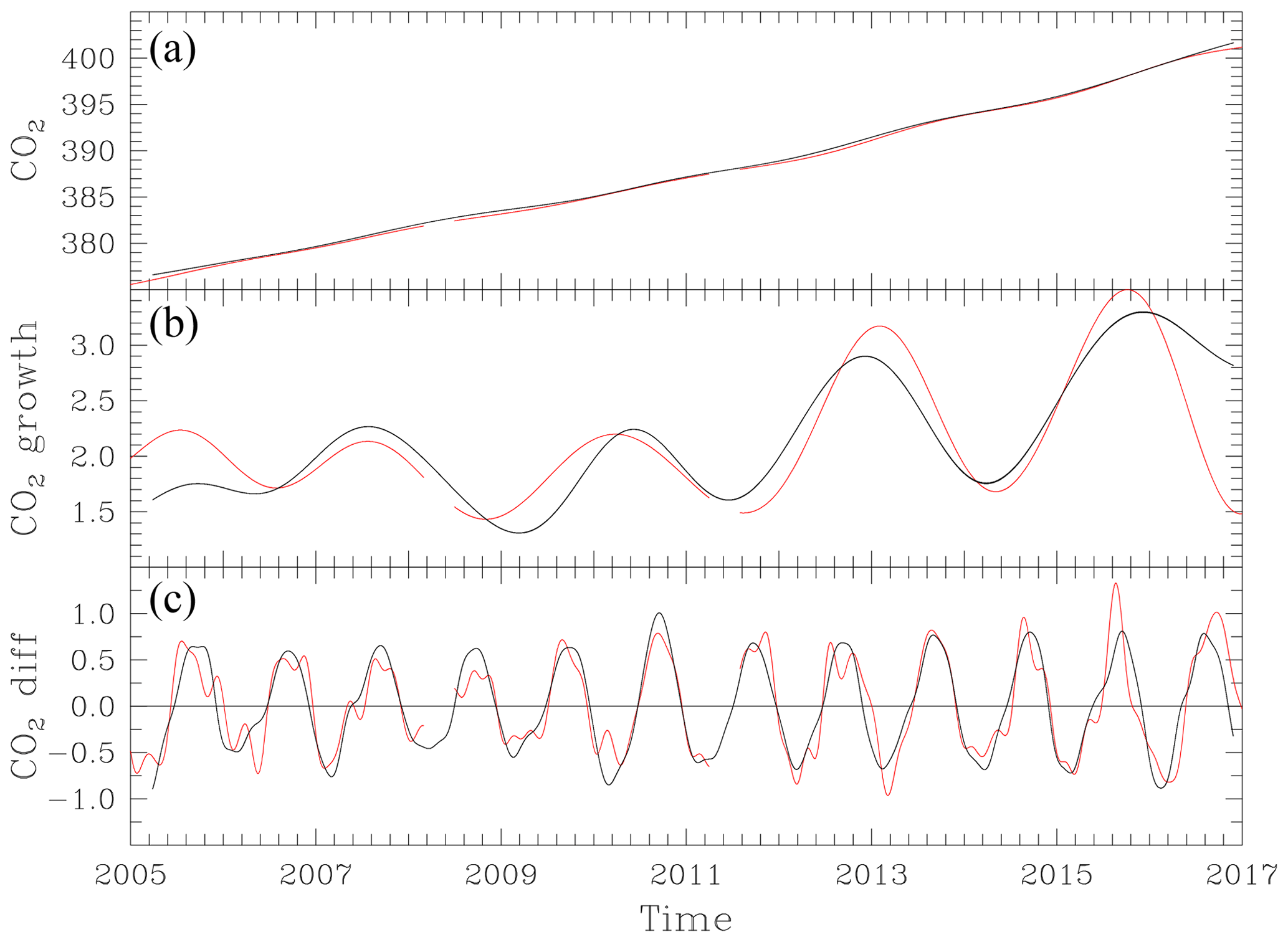
Figure 10 Macquarie Island CO₂ long-term trend in µmol mol⁻¹ (a) and growth rate in $\mathrm{\mu }\mathrm{mol}{\mathrm{mol}}^{-\mathrm{1}}{\mathrm{yr}}^{-\mathrm{1}}$ (b) and difference between the smoothed curve data set and the long term trend in $\mathrm{\mu }\mathrm{mol}{\mathrm{mol}}^{-\mathrm{1}}{\mathrm{yr}}^{-\mathrm{1}}$ (c) using fits to hourly frequency LoFlo data (black) and flask data (red).

6.1 Long-term trend and growth rate

The long-term trend in MQA LoFlo CO₂ is represented by the sum of the second-degree polynomial fit and the 667-day filtered residuals. This is shown in Fig. 10a along with an equivalent fit to the MQA flask measurements. The long-term trends are very similar, with a gradual increase in baseline CO₂ concentrations over the 8-year period from 377 to 392 µmol mol⁻¹. The derivative of the long-term trend, the CO₂ growth rate, is shown in Fig. 10b and here the subtle differences in the long-term trend between the LoFlo and flask records become more evident. From 2006 to 2010 the growth rate from the flask record is less variable than from the LoFlo record, while there is much better agreement for the 2010–2013 period. Figure 7 showed that around 2008 the differences between flask and LoFlo measurements were more negative than for other periods, which is coincident with generally longer storage times and hence larger storage corrections. It is possible that a small bias in flask measurements until 2008 is sufficient to influence the derivative of the long-term trend during 2007–2009. This highlights the sensitivity of the growth-rate calculation to small, systematic biases in observed mole fraction, to which the flask record is much more susceptible than the in situ LoFlo record.

6.2 Seasonal cycle

The seasonal variation in CO₂ at Macquarie Island (Fig. 10c) is conventionally revealed by removing the long-term trend curve from the curve fit that combines the fitted polynomial plus harmonics with the 80-day filtered residuals. The seasonal cycle has a peak to trough amplitude of around 1.5 µmol mol⁻¹ with a minimum around February–March and a maximum around October. There are interannual variations in the seasonality, perhaps more in amplitude than phase, which are mostly picked up in both the LoFlo and flask records. The LoFlo produces a much smoother and more reliable representation of the seasonal cycle over the Southern Ocean than the flask record. This is due both to the higher precision of the data and their much higher temporal frequency. The comparison between seasonal fits clearly shows the limitations of the MQA flask data, despite the very clean Southern Ocean environment. The combination of small but unresolved synoptic variability in CO₂ mole fraction and the necessity of making large storage corrections to the flask data, means that the smooth curve fit, generated with standard fitting parameters, contains unrealistic features. An increase in the short-term filter length may be appropriate to provide a smoother fit. The shortcomings in the flask record have implications for how these data are used in CO₂ inversions, either as individual flask measurements or as averaged or smoothed values. It is also likely that a larger uncertainty should be applied to these data than has typically been used.

It is important to note that the interpretation of the interannual variations in the MQA LoFlo seasonality cannot only consider interannual variations in Southern Ocean fluxes. Tropical and Northern Hemisphere fluxes also make a significant contribution to seasonality across the Southern Ocean (e.g. Law et al., 2006) and that contribution will be influenced by interannual variability in interhemispheric transport (e.g. Francey and Frederiksen, 2016). While this remote contribution complicates the interpretation of the seasonality at a single Southern Ocean site, such as Macquarie Island, comparisons between the seasonality of different Southern Ocean sites may be more revealing. The high precision of the MQA LoFlo record, the equivalent LoFlo record at Cape Grim and the cavity ring-down spectroscopic records at Casey Station, Antarctica now make these across-Southern-Ocean comparisons possible and this is a focus of ongoing research.

7 Conclusions

The Southern Ocean plays a key role in the global CO₂ cycle but studies investigating the variability and seasonality of the sink have been limited by the paucity of both atmospheric and oceanic CO₂ data in the region with sufficient precision to resolve the small but large-scale atmospheric variation. The observations presented here are a new data stream from a key location within the Southern Ocean region that can contribute to the investigation of Southern Ocean CO₂ flux variability and atmospheric transport. Estimates of the uncertainty associated with this record are typically small and dependent on the intended end application of the data set. They vary with the temporal averaging period, the network choice and the magnitude of the sample-reference difference. For applications that compare LoFlo data sets within the CSIRO network, the uncertainty in 30 min mean samples with mole fractions near the reference standard (>99.9 % of all observations) is 0.025 µmol mol⁻¹, allowing reliable measurement of spatial gradients across the Southern Ocean.

The in situ nature of this record (unlike the traditional flask measurements) results in an increase in the temporal frequency of the data and hence a far richer data stream. The in situ record and its statistically derived products (baseline, growth rate, long-term trend and seasonality) are consequently more robust than those of the co-located flask record, which is also impeded by long sample storage times. The increased temporal frequency has revealed diurnal and synoptic variations in atmospheric CO₂ at Macquarie Island which will be explored further in future work. In particular, the combination of this record with other high-precision in situ sites will allow the quantification of small but significant spatial gradients across the Southern Ocean.