the Creative Commons Attribution 4.0 License.
the Creative Commons Attribution 4.0 License.
 | 28 Feb 2019
An improved low-power measurement of ambient NO2 and O3 combining electrochemical sensor clusters and machine learning
Kate R. Smith
Peter D. Ivatt
James D. Lee
Freya Squires
Chengliang Dai
Richard E. Peltier
Mat J. Evans
Alastair C. Lewis
Low-cost sensors (LCSs) are an appealing solution to the problem of spatial resolution in air quality measurement, but they currently do not have the same analytical performance as regulatory reference methods. Individual sensors can be susceptible to analytical cross-interferences; have random signal variability; and experience drift over short, medium and long timescales. To overcome some of the performance limitations of individual sensors we use a clustering approach using the instantaneous median signal from six identical electrochemical sensors to minimize the randomized drifts and inter-sensor differences. We report here on a low-power analytical device (< 200 W) that is comprised of clusters of sensors for NO2, Ox, CO and total volatile organic compounds (VOCs) and that measures supporting parameters such as water vapour and temperature. This was tested in the field against reference monitors, collecting ambient air pollution data in Beijing, China. Comparisons were made of NO2 and Ox clustered sensor data against reference methods for calibrations derived from factory settings, in-field simple linear regression (SLR) and then against three machine learning (ML) algorithms. The parametric supervised ML algorithms, boosted regression trees (BRTs) and boosted linear regression (BLR), and the non-parametric technique, Gaussian process (GP), used all available sensor data to improve the measurement estimate of NO2 and Ox. In all cases ML produced an observational value that was closer to reference measurements than SLR alone. In combination, sensor clustering and ML generated sensor data of a quality that was close to that of regulatory measurements (using the RMSE metric) yet retained a very substantial cost and power advantage.
- Article
(2520 KB) - Full-text XML
- BibTeX
- EndNote


Low-cost sensors (LCSs) are an attractive prospect for use in complex urban environments where more atmospheric measurements are required to build up a better-resolved map of highly heterogeneous pollution patterns. There are numerous reports of low-cost, low-powered sensors commercially available for most of the criteria pollutants. Air pollution measurement has been historically a heavily regulated analytical environment. Many countries have extensive programmes of air quality measurement, and measurements are often situated within a legal framework with prescribed methods of measurement. Air quality monitoring stations use relatively power-intensive equipment, have a high start-up cost and require skilled personnel for calibration and maintenance. A consequence is that, even in wealthy countries, observations are sparse with sites often located 1–10 km2 apart (McKercher et al., 2017). Pollutants often exhibit steep spatial concentration gradients over short distances (Broday et al., 2017), and limited measurement locations mean hotspots are often missed (Mead et al., 2013).
LCSs provide an opportunity to increase the density of atmospheric measurements and reduce the uncertainty that arises when interpolating between current reference monitors. This has many uses, most notably allowing better validation of atmospheric models (Broday et al., 2017). The lower-power and size associated with LCSs, along with high-frequency measurements, makes them an attractive prospect for mobile use and for personal exposure assessment (Williams et al., 2013). Many low-cost sensors are commercially available, either as stand-alone sensors or as multisensory platforms (Caron et al., 2016; Jiao et al., 2016) (for example, AQMesh; Broday et al., 2017). There has been a rapid expansion in the number of publications evaluating such devices recently. Single devices containing sensors for the measurement of criteria pollutants such as CO, NO2, total volatile organic compound (VOC) and O3 cost a fraction of the price (approximate sensor box cost is GBP 5000) of establishing an equivalent measurement site with reference instruments (Mead et al., 2013) (GBP 200 000). Perhaps more importantly sensors can be placed in locations where power is limited or can only be generated through solar resources. The operating costs of low-power devices are also a very attractive feature.
However, the literature contains many examples of where LCS approaches can suffer from relatively poor analytical performance when compared against the reference instruments. Whilst such a comparison is perhaps not always appropriate to make in such a highly regulated field of measurement, the benchmark test of any new analytical device will be against the regulatory reference. Significant uncertainty in measurements is introduced because individual sensors each have a unique response to simple environmental conditions such as humidity and temperature (Smith et al., 2017; Moltchanov et al., 2015). This can lead to a relatively high degree of inter-sensor variability and response drift (Lewis et al., 2016; Spinelle et al., 2017) over durations as short as a few hours (Jiao et al., 2016; Masson et al., 2015), rendering in-laboratory calibrations (where the interfering variables are controlled or non-existent) ineffective (Smith et al., 2017). Electrochemical (EC) sensors can display some chemical cross-interferences with other pollutants that are likely to be present (Mead et al., 2013; Lewis et al., 2016; Masson et al., 2015), and accounting for these can be difficult when the relative concentration ratios of the target measurand and interferences change. Metal oxide sensors (MOSs) often lack selectivity and provide only a rough bulk measure of a particular pollutant class such as VOCs, and the responses generated can depend on the chemical content of the mixture presented to the sensor.
Although some LCS vendors supply a factory calibration with their sensors, these are not always applicable in the real world, where ambient conditions are substantially different to the calibration conditions in the factory. Previous studies have shown that sensors co-located with reference instruments can be used to reproduce typical pollution patterns (Jiao et al., 2016; Mead et al., 2013), but there is a significant challenge when attempting to calculate absolute pollutant concentrations with a single deployed sensor device. Recent efforts using multivariate regression models (Zampolli et al., 2004) and pattern recognition analysis (Jiao et al., 2016) have characterized these responses to the environmental conditions and provided insight into processes that generate the sensor signal (Zampolli et al., 2004; Hong et al., 1996). Thus far, there is no agreed standard calibration or correction procedures for sensor data, or indeed what data standards low-cost sensor data should work towards. For reference monitors in the UK, NOx, CO and O3 instruments must produce reproducible measurements for 3 months that are within 5 % of the average for a certain concentration in the field and results that are linear over a set range (EU, 2008). For NOx this is 0–2000 ppb, for O3 this is 0–500 ppb and CO this is 0–50 ppm to ensure that both rural and urban concentration ranges are taken into account. Although the target performance of low-cost sensors is highly application dependent, these standards do provide a guide for comparison and highlight the need not only for high-accuracy measurements but also reproducibility over long (months) timescales. In order for low-cost sensors to be used in atmospheric monitoring or research applications the uncertainty and reproducibility must be quantified across a range of likely environmental conditions.
If regulatory reference methods are taken as the benchmark, the implication with current single sensors would be very frequent calibration, possibly hourly or daily. Previous work shows that clustering sensors and using the median sensor signal of the cluster can help minimize some of the effect of medium-term noise and limit the effects of inter-sensor variability (Smith et al., 2017). This practice was adopted here during the building and development of a multi-sensor instrument deployed alongside reference instruments.
2.1 Analytical description of the instrument
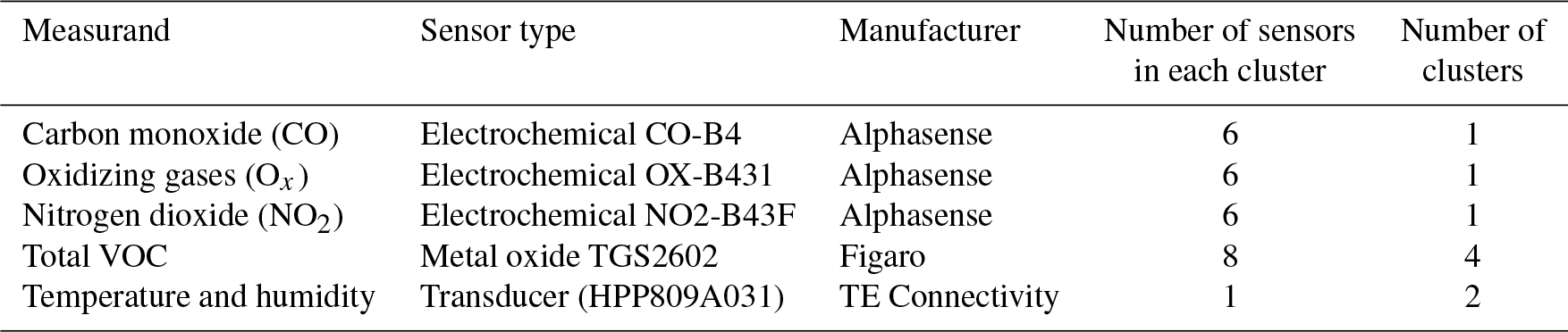
A range of different sensors were mounted into sealed flow cells such that the sensing element of each was exposed to a continually flowing sample of air. The flow cells were in turn installed inside in a 4U aluminium box (177 mm H × 460 mm D ×483 mm W), which had a metal partition to keep the sensors shielded from electrical interference from the pumps and power supplies (Fig. 1). The number of sensors and their type are shown in Table 1.
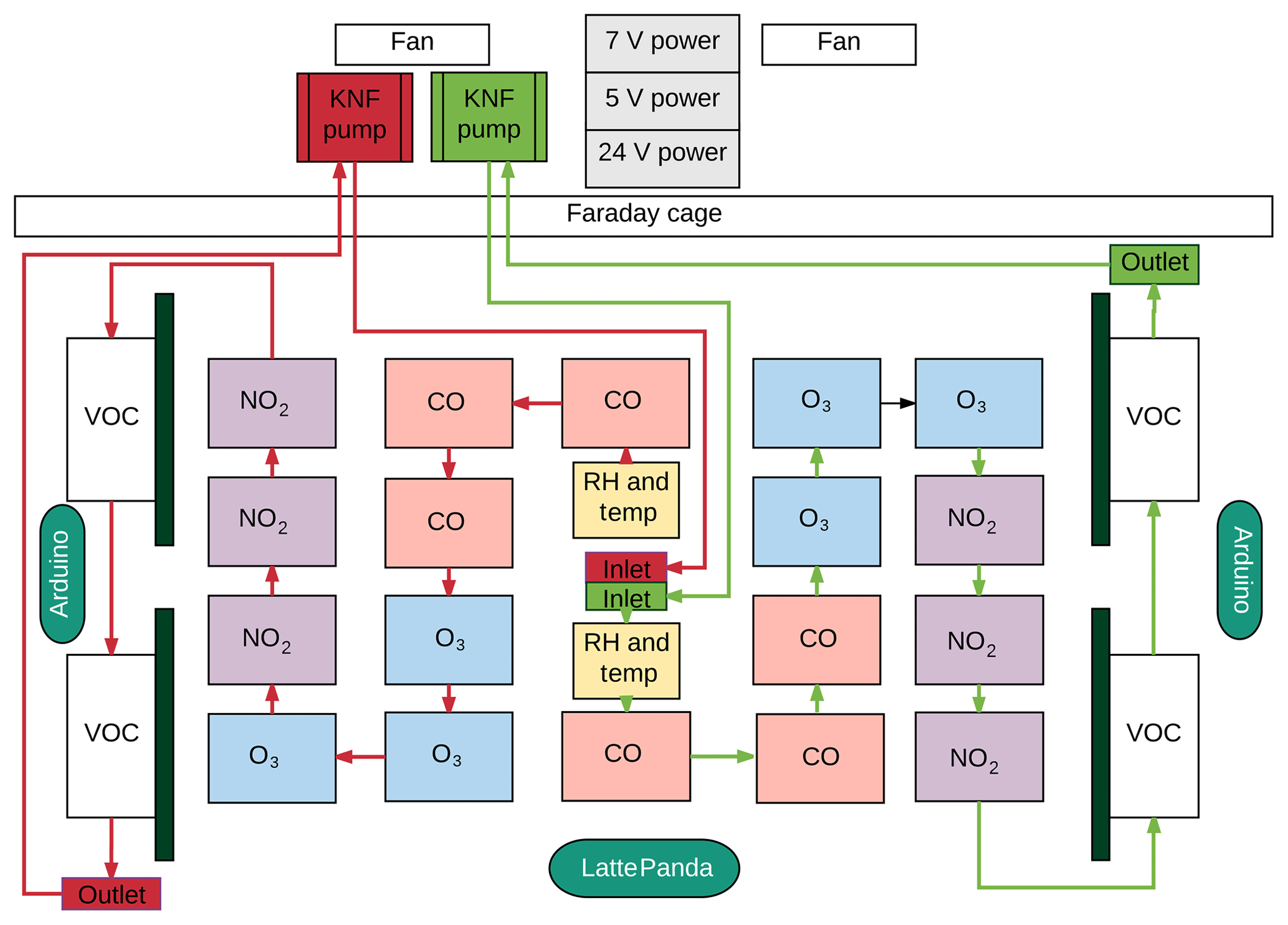
Figure 1Schematic representation of the gas flow paths and basic layout of the sensors and components within the device.
Two microcontrollers (Arduino Uno) were used to collect the data from the sensors. Each Arduino recorded 3 Hz data from 25 sensors, and this was then averaged to 2 s and sent to a LattePanda mini-computer for formatting and storage. Two KNF pumps drew ambient air through a sample line at atmospheric pressure over the sensors at a constant rate (ca. 4 L min−1). Two fans were installed on the box panels to pull air through the box in an attempt to reduce instrument overheating. The power supplies were selected for their low electrical noise, and Adafruit ADS1115 16-bit ADC (analogue-to-digital converter) boards further minimized this issue. A schematic of the instrument is shown in Fig. 1. The overall power budget of the device when operating was approximately 52 W, with a breakdown of components as follows: 18 EC sensors, 9 W; 32 MOSs and internal heaters, 9.4 W; two relative humidity and temperature sensors, 0.01 W; two diaphragm pumps, 16.8 W; two fans, 2.8 W; two Arduino Uno microcontroller boards, 0.58 W; LattePanda micro-computer, 10 W; three power supplies, 3 W.
We note that this type of approach differs from the majority of LCS air quality instruments described in the literature and that are commercially available. In most cases the emphasis in LCS design has been minimizing cost and size. Clearly an instrument that contains > 40 individual sensors is not optimized with cost or size as its main design goals. Instead, we have focused on data reliability as well as the advantages associated with electrical power consumption compared against a suite of traditional reference instruments.
Figure 2 summarizes in simple terms how device costs and power consumption compare between a single sensor device, a six-sensor clustered approach and a reference instrument, using the example of ozone. The clustered approach, whilst more expensive than a single sensor, retains a very substantial power advantage over the reference, creating potential for deployment in remote or off-grid locations, or in developing countries where electrical supplies can be both costly and unreliable. The next key question therefore is whether a more complex and expensive clustered sensor instrument can meet similar data quality as reference instruments and therefore offer a direct alternative but with lower power and operational costs.
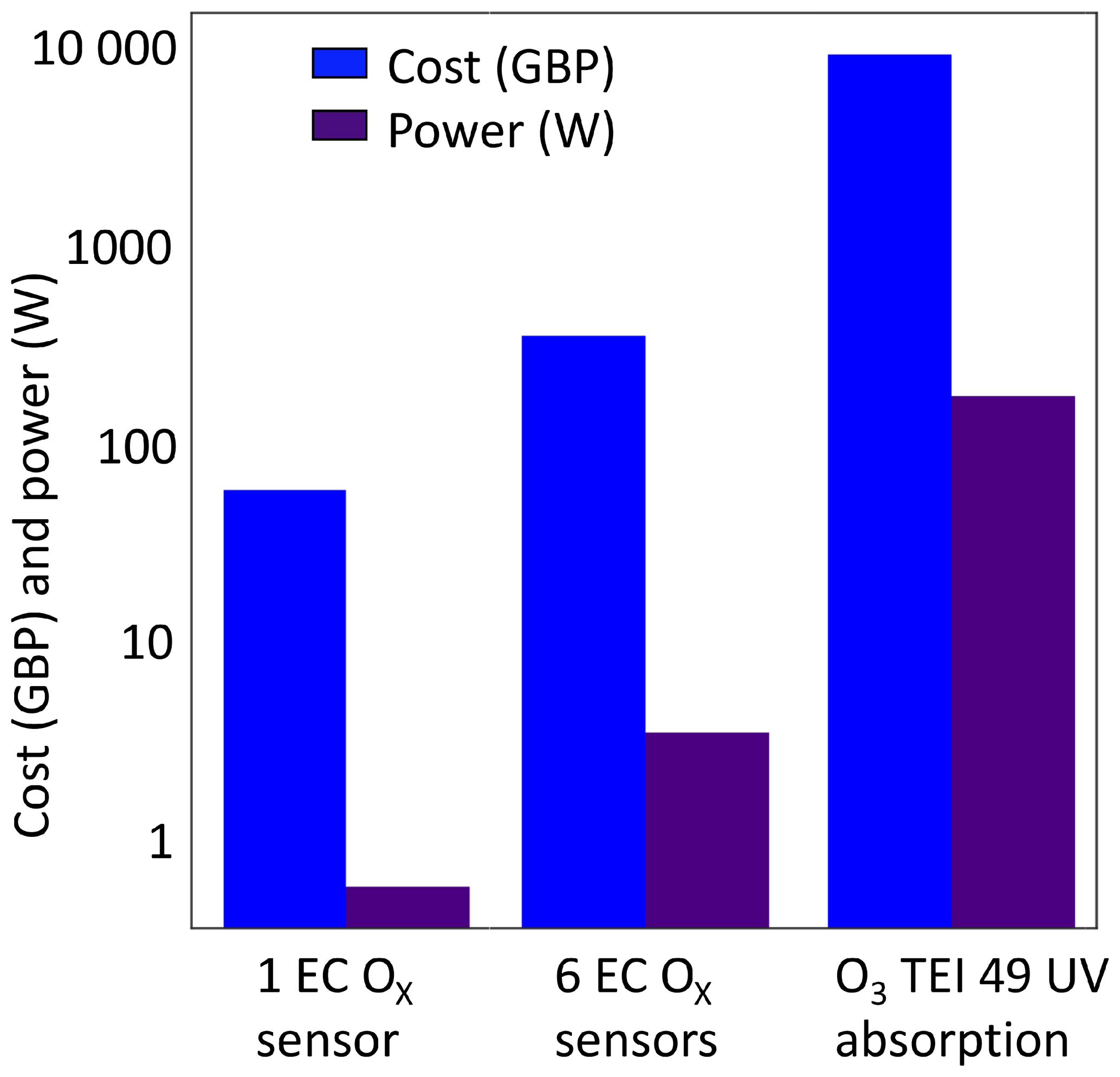
Figure 2Cost (blue) and power (purple) competitiveness for a single Ox EC sensor device, a clustered six-sensor device and a reference UV ozone monitor.
2.2 Sensor test deployment in Beijing
The multi-sensor instrument described in Sect. 2.1 was deployed alongside research-grade reference instruments in Beijing, China, during a large air quality experiment between 29 May and 26 June 2017. Beijing has well documented issues with air quality (Zhang et al., 2016) meaning concentrations of pollutants were anticipated to be elevated and to show a large dynamic range. Beijing also experiences warm, humid summers (Chan and Yao, 2008); during the deployment reported here, air temperature fluctuated between 15.6 and 41.2 ∘C and absolute humidity ranged between 3.82 and 17.83 g m−3. In combination these conditions provide a robust and wide-ranging test of instrument performance.
Both sensors and reference instruments were located at the Institute of Atmospheric Physics (IAP) site (latitude 39.978, longitude 116.387), which is situated to the north of central Beijing. All instruments were housed in converted sea container laboratories for this study. Reference instruments for NO2 and Ox were co-located and sampled from the same 3 m high inlet, with sample bypass flow provided by a common diaphragm pump. The NO2 reference measurement was by cavity-attenuated phase shift (CAPS) spectroscopy (Teledyne T500U, Teledyne, California), with a 100 ppb NO2 in N2 calibration source. The NO2 reference measurements had 5 % uncertainty and 0.1 ppbv precision. O3 reference was measured at 1 min averages by a Thermo Scientific UV absorption photometer (Model 49i), traceable for calibration to the UK National Physical Laboratory primary ozone standard with an uncertainty of 2 %, and a precision of 1 ppb. The sensor instrument collected continuous data as part of the Beijing campaign (Edwards et al., 2017).
2.3 Data analysis approaches
The approach of clustering low-cost sensors was used to improve sensor reproducibility as previously discussed in (Smith et al., 2017), whereas the simple linear regression (SLR) and machine learning (ML) techniques were applied to improve sensor accuracy by correcting for cross-sensitivities.
The median voltage signal from of each of the sensor clusters was calculated automatically by the built-in computing device and software, and then that value converted to concentration units using four different numerical techniques: (i) SLR, (ii) boosted regression trees (BRTs), (iii) boosted linear regression (BLR) and (iv) Gaussian process (GP).
ML techniques (methods ii–iv) are powerful tools for identifying relationships between variables and have been shown to support improved concentration estimates that correct interferences in low-cost sensors (Geron, 2017; Zimmerman et al., 2018; Lin et al., 2018; Esposito et al., 2016; Hagan et al., 2018).
The full dataset from all sensors (chemical and environmental) was used in the ML algorithms with a subset of the time series (2–8 June 2017) treated as training data. Following training, the ML algorithms were then applied to the testing dataset (8–26 June 2017), outputting a corrected concentration value. The median of each sensor cluster of CO, NO2, O3, VOC, plus humidity and temperature, were used by the three different ML algorithms to determine the viability and relative performance of supervised, self-optimization techniques as a method for correcting for cross-interferences. Examples of both parametric (BLR and BRT) and non-parametric (GP) techniques were assessed. BRT was chosen as a numerical method since it provides diagnostics about how the decision trees are constructed, essentially identifying which sensor signals are used in the calculation (Chen and Guestrin, 2016; Geron, 2017). The results can then be compared to known relationships from previous laboratory studies, ensuring that the prediction is in large part a measurement rather than a model value. GP was used because of its proven ability to handle noisy data and it ability to provide the estimations of uncertainty for each data point in the testing data (Geron, 2017; Rasmussen and Williams, 2006).
3.1 How clustering improves performance
Previous laboratory studies (Smith et al., 2017) have shown that clustering sensors was one potential technical approach to reduce the effects of hour to day drift in individual sensor response and limit the effects of inter-sensor manufacturing variability. The median sensor signal was shown to be a more reliable predictor of the true pollutant value (vs. the mean), and the effect of deteriorating or highly variable sensors was minimized. This approach has been extended here to field observations and to a wider range of different chemical species. The EC sensors output two voltages: one from the working electrode (WE) and one from the auxiliary electrode (AE). The standard calibration procedure subtracts the effect of the auxiliary electrode from the working electrode (the electrode exposed to the ambient air and oxidizing compounds) effectively helping to correct for some of the temperature and humidity effects. The manufacturer supplies individual conversion factors and equations for each sensor and these were applied to each sensor prior to use within the cluster. Each sensor within a cluster was initially normalized to give a common voltage output.
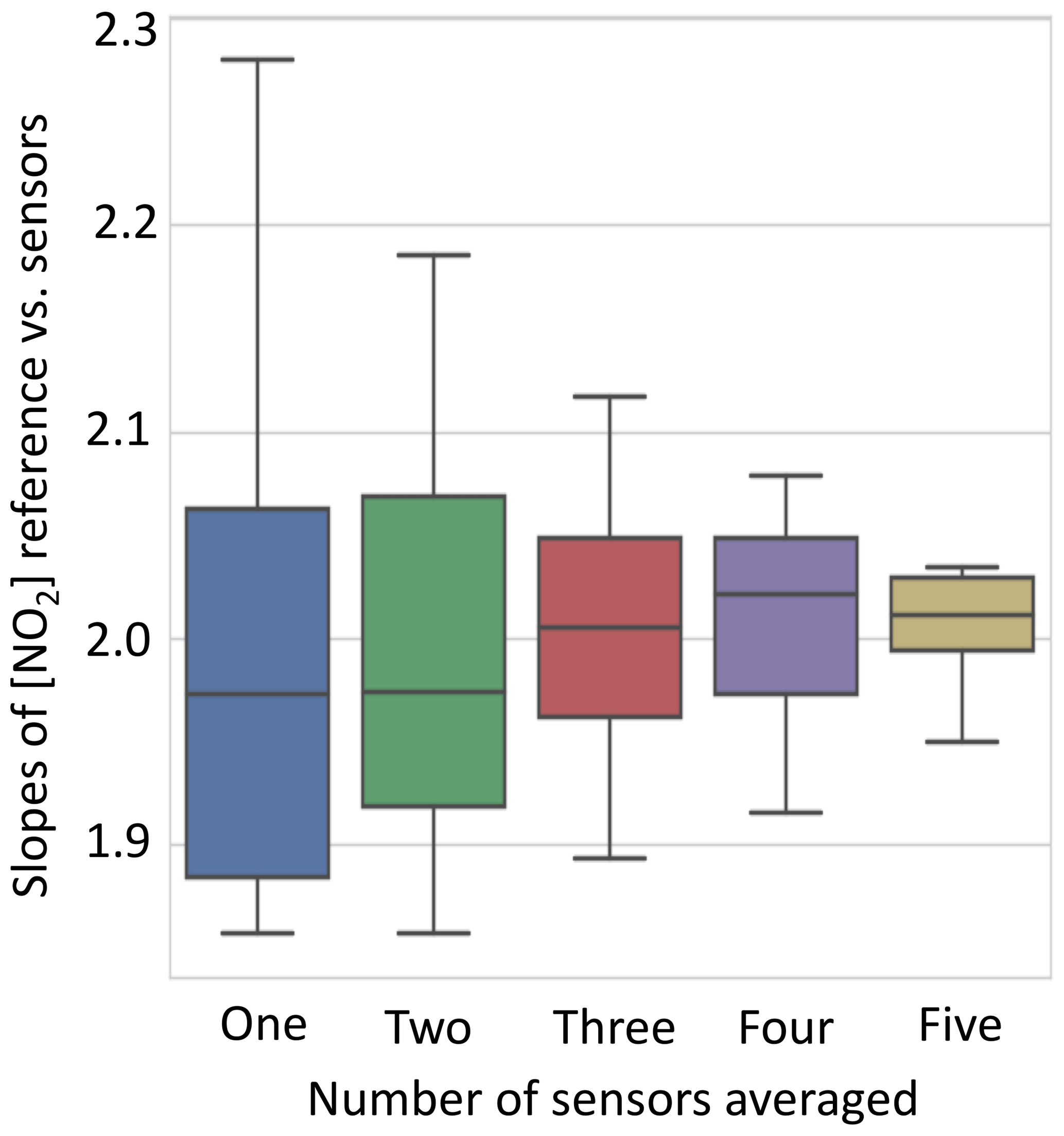
Figure 3Comparison of slopes of concentrations derived from clusters of NO2 EC sensors against a reference instrument for ambient Beijing air. As the number of sensors used increases, the spread in data narrows, as seen through the difference in slope. If data from three out of six sensors are used there are 20 possible permutations of sensors. The average signal of each was calculated, then plotted against the reference NO2 CAPS measurements, and the gradient was extracted. The 20 gradients of these correlation plots (sensitivities) are then plotted in the box plots above, with the median, 25th percentile, and 75th percentile in the box and the 5th and 95th percentile on the whiskers.
We use the raw sensor voltages and the manufacturer's calibration values to gain an initial concentration. One method of determining the improvement in the concentration estimated by the sensors is to compare the range of slopes obtained against reference instrument for a range of different numbers of sensors. This is shown for the first time for an electrochemical NO2 sensor in Fig. 3. As the number of sensors in a cluster is increased, the observed range of values for the unique permutations of the groups narrows considerably, greatly improving measurement precision. The slope does not, however, converge on 1:1 since there is a difference in the factory calibration of the sensors compared to the reference instrument. The cluster vs. reference comparison using simple factory calibration can be seen in Fig. 4a.
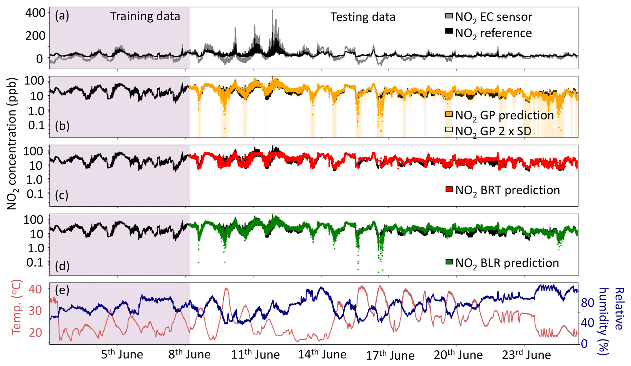
Figure 4(a) Comparison of the median NO2 sensor using individual factory calibrations, (b) the NO2 GP prediction ±2σ, (c) NO2 BRT prediction and (d) NO2 BLR prediction ML techniques. The purple shaded area shows the data used to train the ML algorithms. The black line in all subplots is the York NO2 CAPS measurement, which was used as a reference. Panel (e) shows the relative humidity (%) and temperature (∘C) during the sensor instrument deployment. Note that panels (b), (c) and (d) are plotted with a logarithmic y axis.
3.2 Simple linear regression (SLR)
The first data calibration approach used was SLR, applied to calibrate the median sensor signal using the reference instrument concentration from the first 5 days of the experiment (the training period). The sensor concentrations were corrected using linear parameters from training period calibration, and subsequent sensor performance was assessed by comparing against the co-located reference instrument. Using the NO2 EC sensor cluster as an example, linear parameters in the form of were determined using a linear least-squares fit between the NO2 CAPS reference instrument and the median NO2 EC sensor for the first 5 days of the sensor instrument deployment. Once trained in this manner, these linear calibration factors based on SLR were used to calibrate the median NO2 sensor and were unchanged for the remainder of the experiment.
The different pollutant clusters showed variable performance against their respective reference over the 21 days. We use root-mean-square error (RMSE) here as a metric to evaluate the performance of various clusters and different data calibration approaches. We also calculate the RMSE between two approximately co-located NO2 reference-grade instruments (4.3 ppb) during the same field deployment to quantify what might be considered the “optimum comparison” that could be expected between the sensors and the reference approach. During the campaign a localized source of NO and NO2 was emitted into the vicinity downwind of the second NO2 CAPS instrument and hence not observed by it. For a fair comparison of the two NO2 reference measurements the data between 10 and 14 June, when the localized emissions of NO and NO2 occurred, were removed. Unfortunately, there was not a co-located CO reference instrument or multiple co-located reference observations of O3 available for this study. The CO sensor median was still included with the total VOC median, relative humidity and temperature in the sensor variables for training and testing the ML algorithms, but we were unable to make a comparison.
Applying SLR, the NO2 sensor cluster gave a RMSE of 10.42 ppb and RMSE of 10.44 ppb for the Ox cluster median signal with the sum of the NO2+O3 reference measurements. The ambient NO2 concentrations varied over a wide range from below 2 ppb to in excess of 200 ppb, and the clustered NO2 package performed well at capturing this range of observed concentrations but with substantial discrepancies between the median NO2 EC sensor and the NO2 CAPS reference instrument when the reference NO2 concentrations were below 10 ppb. This finding fits well with previous work that shows the impact of cross-sensitivities on EC sensors is most important at low target compound concentrations (Lewis et al., 2016). The Alphasense OX-B431 sensors detected both O3 and NO2. They respond proportionately but independently to concentrations of O3 and NO2; hence, the Ox EC sensors were calibrated with and compared to the sum of the O3 and NO2 reference measurements. The median value from the Ox cluster showed the best correlation with the respective reference measurements (Ox R2=0.95, NO2 R2=0.86).
3.3 Using machine learning (ML) algorithms to calibrate the median sensor cluster
Each ML algorithm was trained and then tested using the same 1 min average sensor data as the SLR in Sect. 3.2, split into the same training and testing sets each time. The training data were the first 8490 data points of the measurement period, and the testing set was the remaining 25 956 data points. For BRT and BLR the Python XGBoost implementation was used to train, cross-validate and test the models. This scalable learning system is open source, computationally efficient and has performed well on other platforms (Rasmussen and Williams, 2006). Both BRT and BLR have different hyperparameters that allow the ML algorithm to be tuned so that the algorithm can detect trends within the data, without overfitting. Hyperparameters, such as the learning step, can be increased or decreased to allow a good fit to the training data and to optimize the performance of the algorithm (Geron, 2017). To tune the ML algorithm hyperparameters a 5-fold cross-validation of the training set was used to build the classification models, with a randomization seed of 42 each time. The seed randomizes the data, so the value of the seed does not matter, just that it is consistent for the cross-validation. During the cross-validation process, the algorithm trained on one of the five subsets of the training dataset and made a prediction based on these learnt relationships over the other four subsets of data to test out the associated rules it has found. The hyperparameters were decided by minimizing the mean absolute error (MAE) between the predicted subsets of data and the training label (Shi et al., 2017). Once decided, these hyperparameters were fixed and the algorithm then tested on data that it has not yet seen, i.e. the testing dataset.
BRT uses gradient-boosted regression trees to integrate large numbers of decision trees, and this improves the overall performance of the trees (Rasmussen and Williams, 2006; Friedman, 2001). Through a process where many decision trees are working on the training dataset, the algorithm generates a set of rules by which the training data are linked to the training label (Shi et al., 2017). By discarding trees that do not have much impact on the MAE, the algorithm is more efficient at determining the relationships between variables. The nature of decision trees means BRT is not limited to identifying linear functions, unlike BLR. During the same cross-validation process as described for BRT, BLR identifies the linear relationships between the sensor variables and uses these correlations to predict the compound response during the testing period. BLR is simpler than BRT but works well when there are multiple linear trends between variables. GP uses the Gaussian distribution over functions and can be a powerful tool for regression and prediction purposes (Rasmussen and Williams, 2006). It is a flexible model which generalizes the Gaussian distribution of the functions that make up the properties of each variables function (Rasmussen and Williams, 2006). GP can be used as a supervised learning technique once suitable properties for the covariance functions (kernels) are found; then a GP model can be created and interpreted (Roberts et al., 2013). For this study there were two kernels used to train and predict the sensor data. These were matern32 (k1) and linear (k2) functions. They were added together (k1+k2) to enable both linear (k2) and non-linear (k1) relationships between the variables to be detected, as it was observed in the laboratory that the relationships between the variables could be either (Lewis et al., 2016; Smith et al., 2017). The hyperparameters were then self-optimized using the training data by the open-source Python package running the algorithm, GPy. The GP-, BRT- and BLR-predicted responses were then compared to the reference data over the testing period, and a RMSE was calculated to investigate how well the ML algorithm performed.
3.4 Sensor cluster data with ML processing – NO2 cluster
Figure 4 shows the predicted NO2 time series using the median cluster value and the three ML calibrations compared with the reference measurement. The median sensor with individual factory corrections (Fig. 4a) clearly detects the major trend in NO2 concentration but often under-predicts at times when the NO2 concentration is low. At higher concentrations the median sensor over-predicts the NO2 signal, leading to a RMSE of 86.7 ppb.
3.4.1 Gaussian process (GP)
The GP ML algorithm predicted the NO2 concentration with a RMSE of 5.2 ppb compared to the reference measurement, the lowest for all the different ML techniques. The Matern32 kernel is adept at capturing the more typical (sub 50 ppb) NO2 concentrations, due to its ability to model cross-sensitivities on the sensor signals but struggled to extrapolate to highest concentrations. One advantage of using GP to predict compound concentrations is that an uncertainty on the predicted values is also calculated. This uncertainty is shown in Fig. 4b (light yellow shading), as ±2 standard deviations on the predicted data points. It is clear that there are periods when there is more uncertainty in the prediction. There are four main periods where the GP prediction appeared low, and the uncertainty was high: 15:00 UTC on 8 June, 17:00 UTC on 9 June, 14:00 UTC on 15 June and 14:00 UTC on 16 June. These over-extrapolated data points all occurred when the temperature reached 40 ∘C and exceeded the maximum temperature recorded during the training period (35.8 ∘C), coinciding with when the NO2 concentration and relative humidity were low (Fig. 4e). Machine learning techniques all have difficulty making predictions when the testing and training datasets cover different variable space, but the calculation of a prediction uncertainty highlights when this could potentially be an issue and could be used to inform calibration strategies.
3.4.2 Boosted regression trees (BRT)
The BRT prediction (Fig. 4c) was very good during periods when the test data did not exceed concentrations of NO2 seen in the training data (∼79 ppb). However, the classification nature of the BRT algorithm means it is incapable of extrapolation, so the prediction cannot capture the high concentrations of NO2 that were observed between 10 and 14 June (the NO2 CAPS instrument recorded a maximum NO2 concentration of 222.2 ppb during the testing period). During this time a localized source of NO and NO2 was emitted. Overall, the RMSE between the BRT NO2 prediction and the NO2 CAPS reference measurement was 7.2 ppb, an improvement on SLR (10.4 ppb) of ∼30 % despite its inability to capture NO2 concentrations outside of those experienced during the training data period. This improvement for the lower concentrations of NO2 is due to the BRT model's ability to better correct for some cross-sensitivities on the sensor signals, such as the effect of humidity. With the dates omitted for the localized source of NO and NO2 (described in Sect. 3.2) the RMSE for BRT prediction was 6.1 ppb, showing that the BRT prediction does well at capturing the trends in NO2 when extrapolation is not required.
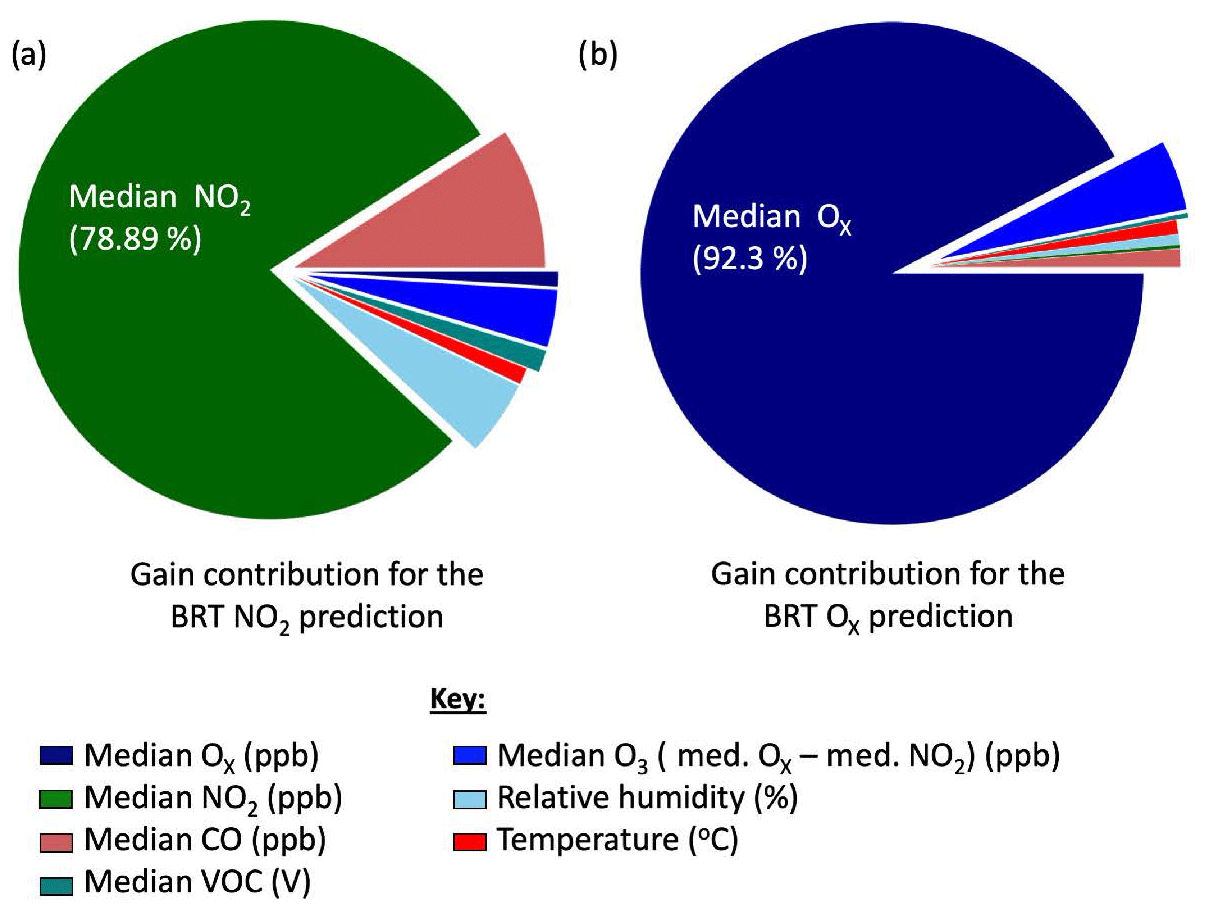
Figure 5Breakdown of contribution from each variable used by the BRT algorithm to predict the clustered (a) NO2 sensor and (b) Ox concentrations.
The BRT algorithm outputs a gain feature called gain, which can be used to identify how much each variable contributes to the predicted sensor response and these are shown in Fig. 5a. The median NO2 sensor signal was (encouragingly) the largest contributor to the NO2 concentration prediction, followed by data from the CO cluster and the relative humidity sensor. This is consistent with previous laboratory results, where it was observed that the NO2 sensor signal had a CO interference and was affected by changing humidity (Lewis et al., 2016).
3.4.3 Boosted linear regression (BLR)
The BLR-predicted NO2 concentration was comparable to the GP prediction, with a RMSE of 6.6 ppb. When the NO and NO2 localized source was removed the RMSE did not change substantially (6.3 ppb) suggesting that this technique was good at extrapolating to the NO2 concentrations outside the range of the training data. BLR assumes purely linear trends between variables, meaning it does not represent non-linear relationships, but the linear nature of the relationships allows BLR to extrapolate trends beyond the ranges seen in the training data. Figure 5d shows the predicted BLR NO2 signal fully capturing the maximum NO2 concentrations between 10 and 14 June. Overall, the RMSE between the BLR prediction and NO2 reference measurement was slightly better than the BRT, suggesting that the inter-sensor relationships were often approximately linear over the variable space observed. The similarity between the GP and BLR predictions is not surprising given the use of the linear kernel in the GP algorithm. The BLR also over-extrapolated the predicted NO2 concentration during the same periods as the GP prediction, suggesting that the linear kernel contributed substantially to the GP prediction but that the training data were not adequate to capture deviations from this linearity.
Table 2The NRMSE and RMSE between the NO2 reference and sensor datasets at different concentration ranges. For each calibration method used in the paper, the data were binned into 25 % of the observed reference concentration. The RMSE and the NRMSE were calculated for each concentration bin and the results for NO2 and Ox are summarized in the table below. The NRMSE was calculated by dividing the RMSE between the reference observations and the sensor values by the mean reference concentration for the respective bin.

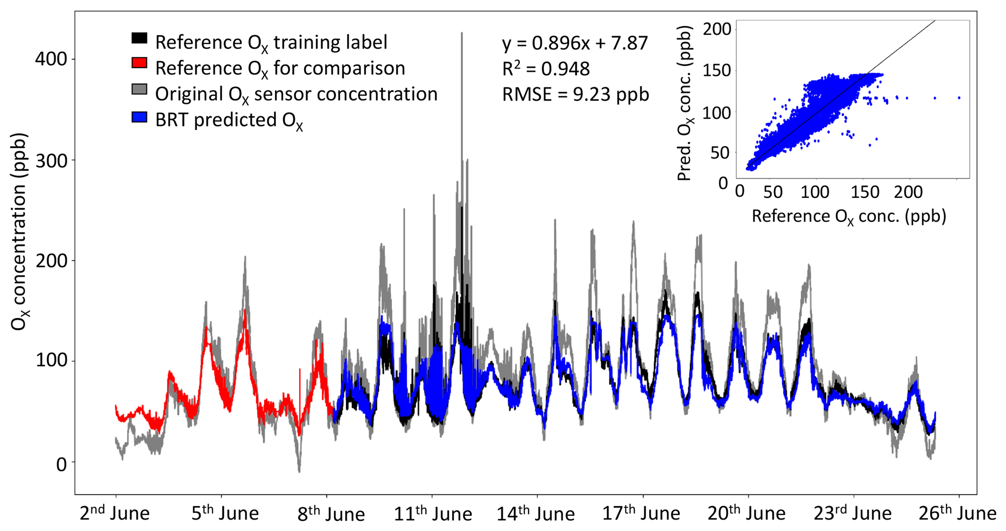
Figure 6Factory-calibrated median sensor concentration (grey), reference O3+NO2 data (black) and BRT Ox prediction (blue) for a cluster of Ox sensors. The reference measurements that were used as the training label are displayed in red. Inset: the correlation plot for the testing dataset, comparing the reference data and the BRT-predicted Ox sensor signal.
Figure 7a summarizes how a progressively improved RMSE can be achieved, as NO2 sensors are first used in a cluster, and then the various different numerical methods are applied to calibration, ultimately producing a performance that is close to the reference vs. reference RMSE. Figure 7a also highlights the evidence that the uncertainty in the sensor concentrations is greatly reduced if the sensors are calibrated in field (using SLR) or if ML procedures are applied. The GP prediction was the ML calibration technique that was closest to the RMSE between the two reference instruments. The RMSE and normalized root-mean-square error (NRMSE) were calculated after the application of SLR and ML for different reference concentration ranges to indicate where the greatest improvement of the sensor data occurred (see Table 2). The RMSE and NRMSE (calculated by dividing the RMSE by the mean of the concentration bin) were determined between the reference NO2 observations and the sensor values for four equally spaced reference concentration bins. The ML techniques produced the greatest improvements in the concentration estimates for the lower concentrations of the target measurand where the effect of cross-interferences is more significant. The BRT and GP in particular displayed large improvements for the lower NO2 reference observations. At the higher concentrations of NO2, the ML algorithms displayed less improvement, where the conditions were outside those of the training data variable space. This was very noticeable for the BRT algorithm due to its inability to extrapolate.
3.5 Sensor cluster data with ML processing – Ox cluster
The data from the median Ox sensor vs. the NO2+O3 reference measurements are shown in Fig. 6, along with the best performing ML data-processing method. During peaks in Ox concentration the factory-calibrated sensor values tend to produce overestimates of the Ox concentrations (e.g. maximum Ox concentration observed by reference was 253 ppb, the median Ox sensor 426 ppb). The ML technique with the lowest RMSE, BRT, brought the Ox concentration estimate much closer to the reference observations (see Fig. 6); however, during peaks in Ox concentration, the BRT-predicted Ox concentration estimate was under-predicted due to BRT's inability to extrapolate.
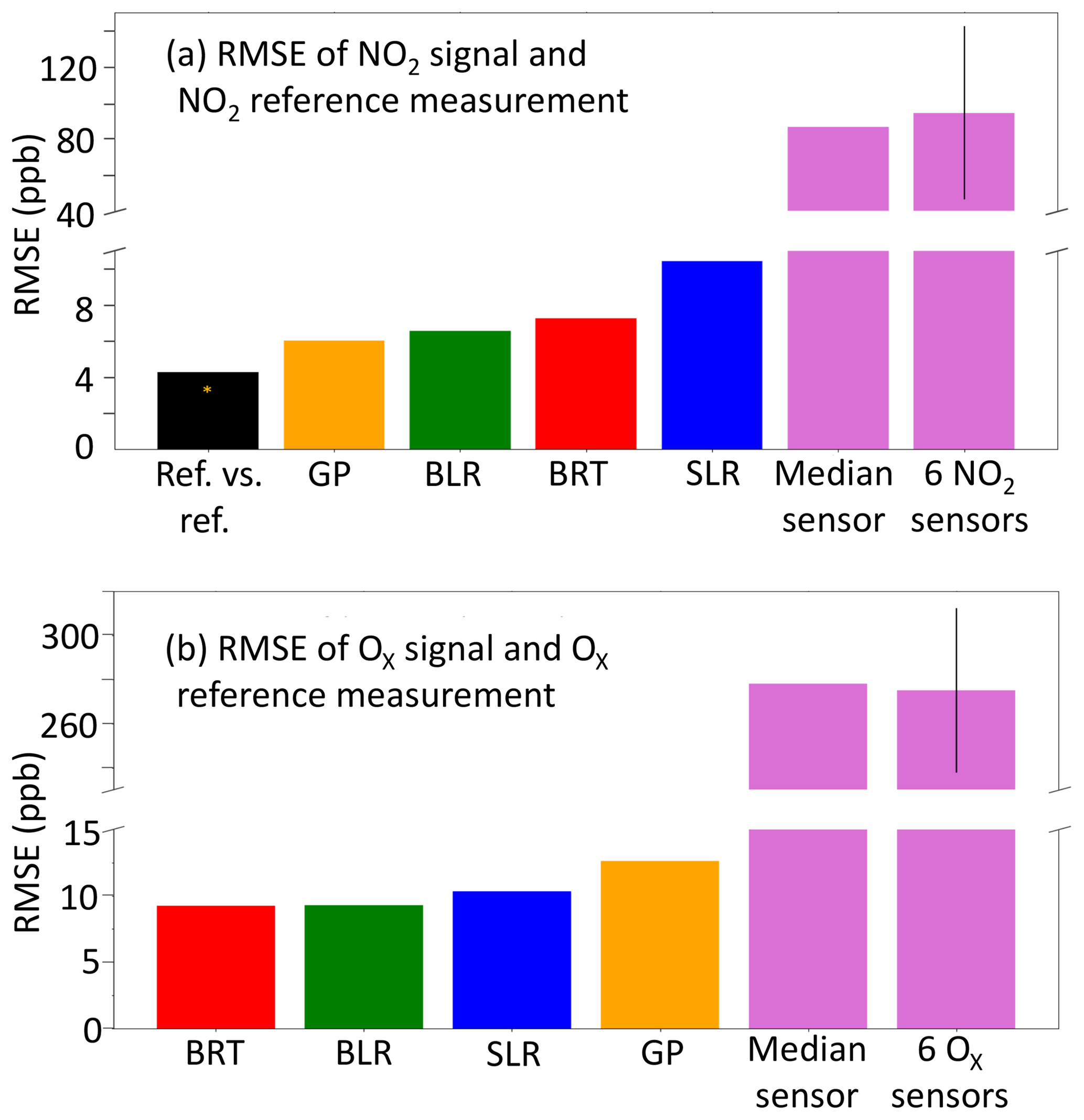
Figure 7Comparison of the RMSE calculated for electrochemical sensor signal data treatment including individual sensors and a cluster of six using factory calibration, SLR and three ML techniques; when available, a reference vs. reference RMSE is also included. (a) NO2; (b) Ox.
A summary of RMSE improvements implemented for all methods can be found in Fig. 7b. BLR and BRT performance was near identical indicating the Ox sensors have largely linear relationships governing their performance, at least over the variable space observed. The 30 % of the data used to train the ML algorithms included a range of Ox concentrations much more representative of the total observation period than was the case for NO2, and so only limited extrapolation beyond the training dataset was needed. The BRT algorithm gain was again used to determine the largest contributing variables to the BRT Ox prediction, Fig. 5b. The median Ox sensor value made the largest contribution to the BRT Ox prediction (92 %). The median CO sensor contributed 1.5 % to the prediction. The NRMSE was calculated for four equally sized reference Ox concentration bins for each analytical method used, in a similar manner to Table 2 for NO2. The NRMSE improved for SLR and the ML algorithms across all concentration ranges, with BLR and BRT optimal for reducing the error estimate the most. The error was the highest at the higher Ox concentrations for BRT, which was expected due to BRT's inability to extrapolate.
3.6 A measurement vs. a sensor model
ML algorithms are skilful at detecting patterns within a dataset, and the work shown in this study is evidence that they can improve the performance of LCSs, as measured by a reported concentration value compared to a reference. Each of the sensor predictions made by the ML algorithms could be justified by previous experience with working with similar EC sensors in the laboratory and from reported studies. For example, the predicted NO2 sensor response was formed based upon decision trees that were primarily influenced by the median NO2 sensor value, and then small adjustments were made to the prediction using the median CO EC and humidity data. This is reasonable based on previous laboratory experiments showing NO2 sensors responding to CO and changing humidity. When using the sensors to correct cross-interferences and changing meteorological conditions, the prediction is an optimized version of the sensor response that essentially calibrates for identified cross-sensitivities.
However, ML algorithms can also be used to make predictions of compounds, for example, nitric oxide (NO), that are simply correlated to other air pollution variables but that are not physically measured by a specific sensor. As an example, in this study a reference-grade NO measurement was made from the same sampling line as the sensor instrument and this was used to make a NO prediction using BRT, based on information gathered by the other chemical sensors. From previous laboratory studies it is known that NO is a cross-interference on the NO2 and Ox EC sensors (Lewis et al., 2016), and therefore we could expect that an NO prediction would use these two variables. However, ambient NO concentrations are closely linked to the concentrations of NO2 and O3 via steady-state interconversion, and this underlying chemistry might also be identified by the algorithm and used to predict NO.
Using a BRT model and sensor cluster median values from the sensor instrument deployment, it was possible to correctly identify when the major NO peaks would occur and predict NO concentrations with a RMSE of 10.5 ppb, even though our instrument did not actually contain a NO sensor. This corresponds to a NRMSE of 0.37. For comparison, the NRMSE for the BRT NO2 and Ox predictions were 0.11 and 0.08, respectively, and the two NO2 reference instruments gave a NRMSE of 0.06, so the NO prediction contains a high degree of uncertainty although appears to be quite good initially. When we interrogate the decision tree model, however, we find that the prediction is largely based on the chemical relationship between NO2 and Ox and not on any cross-sensitivities of sensor signals. In this rather extreme example it could be claimed that this NO prediction is not a measurement but a model (Hagler et al., 2018) and highlights the challenge of interpreting low-cost sensor measurements that exist in something of an analytical grey area due to their reliance on complex calibration algorithms.
Using a combination of clustering sensors and ML data processing, a lower-cost and relatively low-power air quality instrument has made measurements of NO2 and Ox that were close to the RMSE of reference instruments (over the period of study). Clustering of sensors adds little to the overall power budget of an instrument but is a very easy way to overcome individual sensor drift and irreproducibility. Further data treatments such as in-field calibration with SLR or supervised ML techniques can further optimize the sensor data. SLR was seen to improve median sensor concentrations to some degree but struggled to accurately calibrate the sensor data at the lower concentrations. ML techniques were able to further improve the sensor performance because they could correct multiple trends between the sensor variables eliminating some cross-interferences. BLR and BRT were seen to be most powerful at predicting the compound response and used information content from other variables that was reasonable based on previous lab studies. The GP approach was advantageous in that a standard error could be calculated for each predicted data point. Therefore, this identified regions within the data where the prediction was more uncertain, for example, if the testing data significantly deviated from the variable space observed during training. BLR was the simplest technique and worked well when the functions between the sensor variables were linear, for example, during the Ox sensor prediction. The time required to train and run the model was reduced when using BLR and BRT over GP. A longer period of data collection, of at least a few months to a year of sensor data, is needed to establish how long such algorithms accurately predict the reference observations. It appears that as a minimum the use of ML calibration techniques would increase the time required between physical calibrations and allow the use of sensor instruments as part of a network or allow it to run in isolated environments, after the instrument was calibrated over as large a range of conditions, that it is likely to experience, as possible. Data that occur outside the training data ranges can then be flagged and treated with a higher level of uncertainty.
Sensor data for this research have been submitted to the PURE repository and have received the following DOI: https://doi.org/10.15124/1a0c64b0-433b-4eec-b5c7-64d3de0a0351 (Edwards et al., 2017). The reference data can be found on the CEDA website under the Atmospheric Pollution and Human Health in a Developing Megacity (APHH) project.
KRS and PME designed and developed the sensor instrument. KRS, PME, PDI and CD contributed to the analysis of sensor data. FS, JDL and YS provided reference data. All authors contributed to the writing of the manuscript.
The authors declare that they have no conflict of interest.
This article is part of the special issue “In-depth study of air pollution sources and processes within Beijing and its surrounding region (APHH-Beijing) (ACP/AMT inter-journal SI)”. It is not associated with a conference.
This work is supported by AIRPRO grant NE/N007115/1, AIRPOLL grant NE/N006917/1 and NCAS/NERC
ACREW. Peter M. Edwards acknowledges a Marie Skłodowska-Curie Individual
Fellowship. Kate R. Smith and Freya A. Squires acknowledge NERC SPHERES DTP PhDs. Peter D. Ivatt acknowledges an NCAS Studentship PhD. The authors
would like to thank the Institute of Atmospheric Physics, Chinese Academy of
Sciences, and Pingqing Fu for their part in funding the APHH
campaign.
Edited by: Pingqing Fu
Reviewed by: two
anonymous referees
Broday, D. M., Arpaci, A., Bartonova, A., Castell-Balaguer, N., Cole-Hunter, T., Dauge, F. R., Fishbain, B., Jones, R. L., Galea, K., Jovasevic-Stojanovic, M., Kocman, D., Martinez-Iñiguez, T., Nieuwenhuijsen, M., Robinson, J., Svecova, V., and Thai, P.: Wireless distributed environmental sensor networks for air pollution measurement-the promise and the current reality, Sensors, 17, 2263, https://doi.org/10.3390/s17102263, 2017.
Caron, A., Redon, N., Hanoune, B., and Coddeville, P.: Performances and limitations of electronic gas sensors to investigate an indoor air quality event, Build. Environ., 107, 19–28, https://doi.org/10.1016/j.buildenv.2016.07.006, 2016.
Chan, C. K. and Yao, X.: Air pollution in mega cities in China, Atmos. Environ., 42, 1–42, https://doi.org/10.1016/j.atmosenv.2007.09.003, 2008.
Chen, T. and Guestrin, C.: XGBoost: A Scalable Tree Boosting System, Proceedings of the 22nd ACM SIGKDD International Conference on Knowledge Discovery and Data Mining, KDD '16, 13–17 August 2016 San Francisco, CA, USA, https://doi.org/10.1145/2939672.2939785, 2016.
Edwards, P., Smith, K., Lewis, A., and Ivatt, P.: Low cost sensor in field calibrations (training and test data) – Beijing 2017, https://doi.org/10.15124/1a0c64b0-433b-4eec-b5c7-64d3de0a0351, 2017.
Esposito, E., De Vito, S., Salvato, M., Bright, V., Jones, R. L., and Popoola, O.: Dynamic neural network architectures for on field stochastic calibration of indicative low cost air quality sensing systems, Sensor. Actuat. B-Chem., 231, 701–713, https://doi.org/10.1016/j.snb.2016.03.038, 2016.
EU: Directive 2008/50/EC of the European Parliament and of the Council of 21 May 2008 on ambient air quality and cleaner air for Europe, Eur. Union, 152, 1–62, 2008.
Friedman, J. H.: Greedy function approximation: a gradient boosting machine, Ann. Stat., 29, 1189–1232, 2001.
Geron, A.: Hands-On Machine Learning with Scikit-Learn and TensorFlow, First Edit., edited by: Tache, N., Adams, N., and Monaghan, R., O'Reilly Media, Inc., 1005 Gravenstein Highway North, Sebastopol, CA 95472, 2017.
Hagan, D. H., Isaacman-VanWertz, G., Franklin, J. P., Wallace, L. M. M., Kocar, B. D., Heald, C. L., and Kroll, J. H.: Calibration and assessment of electrochemical air quality sensors by co-location with regulatory-grade instruments, Atmos. Meas. Tech., 11, 315–328, https://doi.org/10.5194/amt-11-315-2018, 2018.
Hagler, G. S. W., Williams, R., Papapostolou, V., and Polidori, A.: Air Quality Sensors and Data Adjustment Algorithms: When Is It No Longer a Measurement?, Environ. Sci. Technol., 52, 5530–5531, https://doi.org/10.1021/acs.est.8b01826, 2018.
Hong, H.-K., Shin, H. W., Park, H. S., Yun, D. H., Kwon, C. H., Lee, K., Kim, S.-T., and Moriizumi, T.: Gas identification using micro gas sensor array and neural-network pattern recognition, Sensor. Actuator., 4005, 68–71, 1996.
Jiao, W., Hagler, G., Williams, R., Sharpe, R., Brown, R., Garver, D., Judge, R., Caudill, M., Rickard, J., Davis, M., Weinstock, L., Zimmer-Dauphinee, S., and Buckley, K.: Community Air Sensor Network (CAIRSENSE) project: evaluation of low-cost sensor performance in a suburban environment in the southeastern United States, Atmos. Meas. Tech., 9, 5281–5292, https://doi.org/10.5194/amt-9-5281-2016, 2016.
Lewis, A. C., Lee, J., Edwards, P. M., Shaw, M. D., Evans, M. J., Moller, S. J., Smith, K., Ellis, M., Gillott, S., White, A., and Buckley, J. W.: Evaluating the performance of low cost chemical sensors for air pollution research, Faraday Discuss., 189, 85–103, https://doi.org/10.1039/C5FD00201J, 2016.
Lin, Y., Dong, W., and Chen, Y.: Calibrating Low-Cost Sensors by a Two-Phase Learning Approach for Urban Air Quality Measurement, Proc. ACM Interact. Mob. Wearable Ubiquitous Technol. Artic., 2, 1–18, https://doi.org/10.1145/3191750, 2018.
Masson, N., Piedrahita, R., and Hannigan, M.: Quantification method for electrolytic sensors in long-term monitoring of ambient air quality, Sensors, 15, 27283–27302, https://doi.org/10.3390/s151027283, 2015.
McKercher, G. R., Salmond, J. A., and Vanos, J. K.: Characteristics and applications of small, portable gaseous air pollution monitors, Environ. Pollut., 223, 102–110, https://doi.org/10.1016/j.envpol.2016.12.045, 2017.
Mead, M. I., Popoola, O. A. M., Stewart, G. B., Landshoff, P., Calleja, M., Hayes, M., Baldovi, J. J., Mcleod, M. W., Hodgson, T. F., Dicks, J., Lewis, A., Cohen, J., Baron, R., Saffell, J. R., and Jones, R. L.: The use of electrochemical sensors for monitoring urban air quality in low-cost, high-density networks, Atmos. Environ., 70, 186–203, https://doi.org/10.1016/j.atmosenv.2012.11.060, 2013.
Moltchanov, S., Levy, I., Etzion, Y., Lerner, U., Broday, D. M., and Fishbain, B.: On the feasibility of measuring urban air pollution by wireless distributed sensor networks, Sci. Total Environ., 502, 537–547, https://doi.org/10.1016/j.scitotenv.2014.09.059, 2015.
Rasmussen, C. E. and Williams, C. K. I.: Gaussian Processes for Machine Learning, 2nd Edition, The MIT Press, Cambridge, Massachusetts, 2006.
Roberts, S., Osborne, M., Ebden, M., Reece, S., Gibson, N., and Aigrain, S.: Gaussian processes for time-series modelling, Philos. T. R. Soc. A, 371, 20110550, https://doi.org/10.1098/rsta.2011.0550, 2013.
Shi, X., Li, Q., Qi, Y., Huang, T., and Li, J.: An accident prediction approach based on XGBoost, Conference proceedings 2017, 12th International Conference on Intelligent Systems and Knowledge Engineering (ISKE), 24–26 November 2017, Nanjing, China,, 1–7, https://doi.org/10.1109/ISKE.2017.8258806, 2017.
Smith, K., Edwards, P. M., Evans, M. J. J., Lee, J. D., Shaw, M. D., Squires, F., Wilde, S., and Lewis, A. C.: Clustering approaches that improve the reproducibility of low-cost air pollution sensors, Faraday Discuss., 200, 621–637, 1–17, https://doi.org/10.1039/C7FD00020K, 2017.
Spinelle, L., Gerboles, M., Villani, M. G., Aleixandre, M., and Bonavitacola, F.: Field calibration of a cluster of low-cost commercially available sensors for air quality monitoring. Part B: NO, CO and CO2, Sensor. Actuat. B-Chem., 238, 706–715, https://doi.org/10.1016/j.snb.2016.07.036, 2017.
Williams, D. E., Henshaw, G. S., Bart, M., Laing, G., Wagner, J., Naisbitt, S., and Salmond, J. A.: Validation of low-cost ozone measurement instruments suitable for use in an air-quality monitoring network, Meas. Sci. Technol., 24, 065803, https://doi.org/10.1088/0957-0233/24/6/065803, 2013.
Zampolli, S., Elmi, I., Ahmed, F., Passini, M., Cardinali, G. C., Nicoletti, S., and Dori, L.: An electronic nose based on solid state sensor arrays for low-cost indoor air quality monitoring applications, Sensor. Actuat. B-Chem., 101, 39–46, https://doi.org/10.1016/j.snb.2004.02.024, 2004.
Zhang, H., Wang, S., Hao, J., Wang, X., Wang, S., Chai, F., and Li, M.: Air pollution and control action in Beijing, J. Clean. Prod., 112, 1519–1527, https://doi.org/10.1016/j.jclepro.2015.04.092, 2016.
Zimmerman, N., Presto, A. A., Kumar, S. P. N., Gu, J., Hauryliuk, A., Robinson, E. S., Robinson, A. L., and R. Subramanian: A machine learning calibration model using random forests to improve sensor performance for lower-cost air quality monitoring, Atmos. Meas. Tech., 11, 291–313, https://doi.org/10.5194/amt-11-291-2018, 2018.