Dual-wavelength radar technique development for snow rate estimation: a case study from GCPEx

quantitative precipitation estimation (QPE) of snowfall has generally been expressed in power-law form between equivalent radar reflectivity factor (Z_e) and liquid equivalent snow rate (SR). It is known that there is large variability in the prefactor of the power law due to changes in particle size distribution (PSD), density, and fall velocity, whereas the variability of the exponent is considerably smaller. The dual-wavelength radar reflectivity ratio (DWR) technique can improve SR accuracy by estimating one of the PSD parameters (characteristic diameter), thus reducing the variability due to the prefactor. The two frequencies commonly used in dual-wavelength techniques are Ku- and Ka-bands. The basic idea of DWR is that the snow particle size-to-wavelength ratio is falls in the Rayleigh region at Ku-band but in the Mie region at Ka-band.

We propose a method for snow rate estimation by using NASA D3R radar DWR and Ka-band reflectivity observations collected during a long-duration synoptic snow event on 30–31 January 2012 during the GCPEx (GPM Cold-season Precipitation Experiment). Since the particle mass can be estimated using 2-D video disdrometer (2DVD) fall speed data and hydrodynamic theory, we simulate the DWR and compare it directly with D3R radar measurements. We also use the 2DVD-based mass to compute the 2DVD-based SR. Using three different mass estimation methods, we arrive at three respective sets of Z–SR and SR(Z_h, DWR) relationships. We then use these relationships with D3R measurements to compute radar-based SR. Finally, we validate our method by comparing the D3R radar-retrieved SR with accumulated SR directly measured by a well-shielded Pluvio gauge for the entire synoptic event.

1 Introduction

A detailed understanding of the geometric, microphysical, and scattering properties of ice hydrometeors is a vital prerequisite for the development of radar-based quantitative precipitation estimation (QPE) algorithms. Recent advances in surface and airborne optical imaging instruments and the wide proliferation of dual-polarization and multi-wavelength radar systems (ground based, airborne or satellite) have allowed for observations of the complexity inherent in winter precipitation via dedicated field programs (e.g., Skofronick-Jackson et al., 2015; Petäjä et al., 2016). These large field programs are vital given that the retrieval problem is severely underconstrained due to large number of geometrical and microphysical parameters of natural snowfall, their extreme sensitivity to subtle changes in environmental conditions, and co-existence of different populations of particle types within the sample volume (e.g., Szyrmer and Zawadzki, 2014).

The surface imaging instruments that give complementary measurements and are used in a number of recent studies include (i) 2-D video disdrometer (2DVD; Schönhuber et al., 2008), (ii) precipitation imaging package (PIP; von Lerber et al., 2017), (iii) Multi-Angle Snowflake Camera (MASC; Garrett et al., 2012). When these instruments are used in conjunction with a well-shielded GEONOR or PLUVIO gauge, it is shown that a physically consistent representation of the geometric, microphysical, and scattering properties needed for radar-based QPE can be achieved (Szyrmer and Zawadzki, 2010; Huang et al., 2015; von Lerber et al., 2017; Bukovčić et al., 2018). In this study, we use the 2DVD and PLUVIO gauge located within a double fence international reference (DFIR) wind shield to reduce wind effects.

Radar-based QPE has generally been based on Z_e–SR (Z_e is reflectivity; SR is liquid equivalent snow rate) power laws of the form Z_e=α(SR)^β, where the prefactor and exponent are estimated based on (i) direct correlation of radar-measured Z_e with snow gauges (Rasmussen et al., 2003; Fujiyoshi et al., 1990; Wolfe and Snider, 2012) or (ii) using imaging disdrometers such as 2DVD or PIP (Huang et al., 2015; von Lerber et al., 2017). Recently, Falconi et al. (2018) developed Z_e–SR power laws at three frequencies (X-, Ka-, and W-band) by direct correlation of radar and PIP observations. These studies have highlighted the large variability of α due to particle size distribution (PSD), density, fall velocity, and dominant snow type, whereas the variability in β is considerably smaller. Similarly, both methods, (i) and (ii), have been used to estimate ice water content (IWC) from Z_e using power laws of the form Z_e=a(IWC)^b based on airborne particle probe data, direct measurements of IWC, and airborne measurements of Z_e (principally at X-, Ka-, and W-bands) (e.g., Heymsfield et al., 2005, 2016; Hogan et al., 2006). The advantage of airborne data is that a wide variety of temperatures and cloud types can be sampled (Heymsfield et al., 2016).

The dual-wavelength reflectivity ratio (DWR, the ratio of reflectivity from two different bands) radar-based QPE was proposed by Matrosov (1998), Matrosov et al. (2005) to improve SR accuracy by estimating the PSD parameter (median volume diameter D₀) with relatively low dependence on density if assumed constant. There has been limited use of dual-λ techniques for snowfall estimation, mainly using vertical-pointing ground radars or nadir-pointing airborne radars (Liao et al., 2005, 2008, 2016; Szyrmer and Zawadzki, 2014; Falconi et al., 2018). The dual-λ method is of interest to us due to the availability of the NASA D3R scanning radar (Vega et al., 2014), which, to the best of our knowledge, has not been exploited for snow QPE to date.

The DWR is defined as the ratio of the equivalent radar reflectivity factors at two different frequency bands. The main principle in DWR is that the particle's size-to-wavelength ratio falls in the Rayleigh region at a low-frequency band (e.g., Ku-band) but in the Mie region at a high-frequency band (e.g., Ka-band) (Matrosov, 1998; Matrosov et al., 2005; Liao et al., 2016). Previous studies have shown that the DWR can be used to estimate D_m, where D_m is defined as the ratio of the fourth moment to the third moment of the PSD expressed in terms of liquid-equivalent size or mass (Liao et al., 2016). In this sense the DWR is similar to differential reflectivity (Z_dr) in dual-polarization radar technique, where Z_dr is used to estimate D_m (but the physical principles are, of course, different; Meneghini and Liao, 2007). The SR is obtained by “adjusting” the coefficient α in the Z_e–SR power law based on the estimation of D_m provided by the DWR. The prefactor α depends on the intercept parameter of the PSD (von Lerber et al., 2017) and not on D_m directly. However, because of the apparent negative correlation between D_m and PSD intercept parameter for a snowfall of a given intensity (Delanoë et al., 2005; Tiira et al., 2016), measurements of D_m can be used to adjust the Z_e–SR power law.

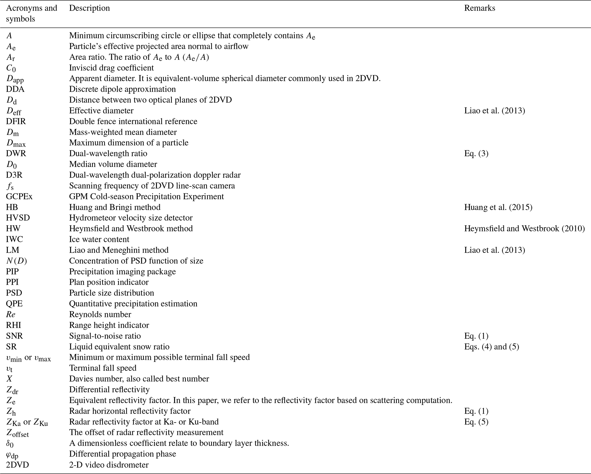
This paper is organized as follows. In Sect. 2, we introduce the approach and methodologies proposed and used in this study, which may be considered technique development. We briefly explain how to estimate the mass of ice particles using a set of aerodynamic equations based on Böhm (1989) and Heymsfield and Westbrook (2010). We also give a brief introduction of the scattering model based on particle mass. Section 3 provides a brief overview of instruments installed at the test site and the dual-wavelength radar used in this study (D3R: Vega et al., 2014). We analyze surface and D3R radar data from one synoptic snowfall event during GCPEx and compare SR retrieved from DWR-based relations with SR measured by a snow gauge. The conclusions and possibilities for further improvement of the proposed techniques are discussed in Sect. 4. The acronyms and symbols are listed in Appendix.

2 Methodology

2.1 Estimation of particle mass

The direct estimation of the mass of an ice particle is difficult and at present there is no instrument available to do this automatically. The conventional method is to use a power-law relation between the mass and the maximum dimension of the particle of the form m=aD^b, where the prefactor a and exponent b are computed via measurements of particle size distribution N(D) from aircraft probes and independent measurements of the total ice water content as an integral constraint (Heymsfield and Westbrook, 2010). A similar method was used by Brandes et al. (2007), who used 2DVD data for N(D) and a snow gage for the liquid equivalent snow accumulation over periods of 5 min. These methods are more representative of an average relation when one particle type (e.g., snow aggregates) dominates the snowfall with large deviations possible for individual events with differing particle types (e.g., graupel).

To overcome these difficulties a more general method was proposed by Böhm (1989) based on estimating mass from fall velocity measurements, geometry, and environmental data if the measured fall velocity is in fact the terminal velocity (i.e., in the absence of vertical air motion or turbulence and in more or less uniform precipitation). The methodology has been described in detail by Szyrmer and Zawadzki (2010), Huang et al. (2015), and von Lerber et al. (2017), and we refer to these articles for details. The essential feature is the unique nonlinear relation between the Davies (1945) number (X) and the Reynolds number (Re), where X is the ratio of mass to area or $m/A_{\mathrm{r}}^{\mathrm{0.25}}$ ($A_{\mathrm{r}}=A_{\mathrm{e}}/A$ is the area ratio, where A_e is the effective projected area normal to the flow and A is the area of the minimum circumscribing circle or ellipse that completely contains A_e) and the Re is the product of terminal fall speed and the characteristic dimension of the particle. We have neglected the environmental parameters (air density, viscosity) as well as boundary layer depth of Abraham (1970) and the inviscid drag coefficient. The procedure is to (i) compute Re from fall velocity measurements and characteristic dimension of the particle (usually the maximum dimension), (ii) compute the Davies number X, which is expressed as a nonlinear function of Re, and boundary layer parameters (C₀=0.6 and δ₀=5.83; Böhm, 1989) and (iii) estimate particle mass from X and A_r. Heymsfield and Westbrook (2010) proposed a simple adjustment (based on field and tank experiments) by defining a modified Davies number as proportional to $m/A_{\mathrm{r}}^{\mathrm{0.5}}$ along with different boundary layer constants (C₀=0.292; δ₀=9.06) from Böhm. Their adjustment was shown to be in very good agreement with recent tank experiments by Westbrook and Sephton (2017), especially for particles like pristine dendrites with low A_r and at low Re. Note that the difference of C₀ and δ₀ in Böhm and Heymsfield–Westbrook equations is mainly due to differences in the shape-correcting factor (A_r) to find the optimal relation between drag coefficient (or Davies number, X) and Reynolds number (Re). This is the main parameterization error in this set of equations.

2.2 Geometric and fall speed measurements

One source of uncertainty in applying the Böhm or Heymsfield and Westbrook (HW) method is calculating the area ratio (A_r) using instruments such as 2DVD or precipitation instrument package (PIP) as they do not give the projected area normal to the flow (i.e., they do not give the needed top view, but rather the 2DVD gives two side views on orthogonal planes as illustrated in Fig. 1). This is reasonable for snow aggregates which are expected to be randomly oriented. The other source of uncertainty is in the definition of characteristic dimension used in Re, which in the HW method is taken to be the diameter of the circumscribing circle that completely encloses the projected area, the maximum dimension (D_max; this is what we use for the 2DVD in our application of the HW method). For the Böhm method we use the procedure in Huang et al. (2015), which used D_app defined as the equal-volume spherical diameter.

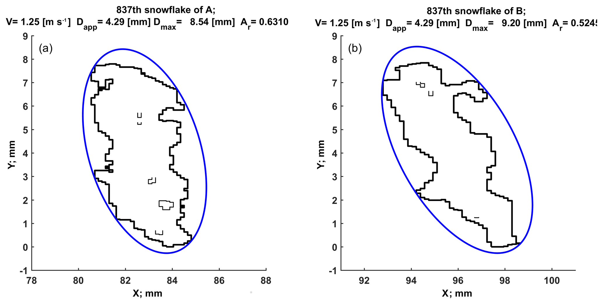
Figure 1 A snowflake observed by a 2DVD from two views. The thick black line is the contour of the snowflake and the thin black lines show the holes inside the snowflake. The effective area, A_e, equals the area enclosed by the thick black curve minus the area enclosed by thin lines. The blue line represents the minimum circumscribed ellipse, the enclosed area of which is denoted by A.

The two-dimensional video disdrometer (2DVD) used herein is described in Schönhuber et al. (2000), and calibration and accuracy of the instrument are detailed in Bernauer et al. (2015). The 2DVD is equipped with two line-scan cameras (referred to as cameras A and B) which can capture the particle image projection in two orthogonal planes (two side views). As mentioned earlier the area ratio (A_r) should be obtained from the projected image in the plane normal to the flow (i.e., top or bottom view). However, to the best of our knowledge, there are no ground-based instruments that can automatically and continuously capture the horizontal projected views (i.e., in the plane orthogonal to the flow) of precipitation particles (however, 3-D-reconstruction based on multiple views can give this information; Kleinkort et al., 2017). Compared with other optical-based instruments, such as HVSD (hydrometeor velocity size detector; Barthazy et al., 2004) or SVI (snow video imager; Newman et al., 2009), which only captures the projected view in one plane, the 2DVD offers views in two orthogonal planes, giving more geometric information. Figure 1 shows a snowflake observed by a 2DVD from two cameras. The thick black line is the contour of the particle and the thin black lines show the holes inside the particle. The effective projected area A_e in the definition of area ratio is easy to compute by counting total pixels from the particle's image, and then multiplying by horizontal and vertical pixel width. The blue line is the minimum circumscribed ellipse. The area of the ellipse is A in the definition of area ratio. The size of particle measured by 2DVD is called the apparent diameter (D_app) which is defined as the diameter of the equivalent volume sphere (Schönhuber et al., 2000; Huang et al., 2015). The D_app is used when computing Re, as mentioned earlier. The area ratio and D_app are the geometric parameters that are used in our implementation of the Böhm method.

In our application of the HW method, the A is based on the diameter of the circumscribed circle that completely encloses the projected pixel area (A_e), which is easy to calculate from the contours in Fig. 1. Thus the area ratio is A_e∕A, while the characteristic dimension in Re is the diameter of the circumscribing circle. Note that the area ratio and characteristic dimension in Re depend on the type of instrument used (e.g., advanced version of snow video imager by von Lerber et al., 2017; the HVSD by Szyrmer and Zawadzki, 2010). These instruments give a projected view in one plane only and thus geometric corrections are used as detailed in the two references.

The two optic planes of the 2DVD are separated by around 6 mm and the accurate distance is based on calibration by dropping 10 mm steel balls at three corners of the sensing area (details of the calibration as well as accuracy of size, fall speed, and other geometric measures are given in Bernauer et al., 2015). During certain time periods, more than one precipitation particle falls in the 2DVD observation area. Since the two cameras look in different directions, the particles observed by camera A and camera B need to be paired. This pairing procedure is called “matching”, and it is illustrated in Fig. 2. The time period [t₁, t₂] is dependent on the assumed reasonable fall speed range. Assuming that the minimum and maximum reasonable fall speeds are v_min and v_max, respectively, the distance between two optic planes is D_d, and camera A observed a particle at t₀, we have $t_{\mathrm{1}}=t_{\mathrm{0}}+D_{\mathrm{d}}/v_{\max }$ and $t_{\mathrm{2}}=t_{\mathrm{0}}+D_{\mathrm{d}}/v_{\min }$. After matching, the fall speed can be calculated as D_d∕Δt, where Δt is the time difference between two cameras observing the same particle. Because the fall speed of the 2DVD is dependent on matching, the geometric features and fall speeds will be in error when mismatch occurs. Huang et al. (2010) analyzed snow data from the 2DVD and found that the 2DVD manufacturer's matching algorithm for snow resulted in a significant mismatching problem (see also Bernauer et al., 2015). In the Appendix of Huang et al. (2010), they showed that the mismatch will cause the volume, vertical dimension, and fall speed of particles to be overestimated. Subsequently, the mass of particles will also be overestimated, mainly because of fall speed. To get the best estimation of mass, they used 2DVD single-camera data and re-did the matching based on a weighted Hanesch criteria (Hanesch, 1999). If the match criteria are not satisfied, then that particle is rejected; it follows that the concentration will tend to be underestimated. To readjust the measured concentration for this underestimate (assumed to be a constant factor), the procedure described in Huang et al. (2015) is used, which only involves the ratio of the total number of particles counted in the scan area of the single camera to the number of successfully matched particles in the virtual measurement area. For the event analyzed here (using method 1 in Sect. 3.3), this adjustment factor is between 1.1 and 1.5. The Pluvio gauge accumulation is not used as a constraint in method 1. The disadvantage of using single-camera data, as described in Huang et al. (2015), is that the particle contour data are not available (i.e., the manufacturer's code does not provide line scan data from single camera). Without contour data, both D_app and A can only be estimated by the maximum width of the scan line and height of the particle as detailed in Huang et al. (2015). Moreover, the diameter of the circumscribing circle or ellipse cannot be obtained without contour data. The only quantity included in single-camera data is A_e in terms of number of pixels. The Huang and Bringi approach (Huang et al., 2015) is referred to as HB, because both PSD (particle size distribution) and reflectivity (Z_e) are computed using D_app as the measure of particle size.

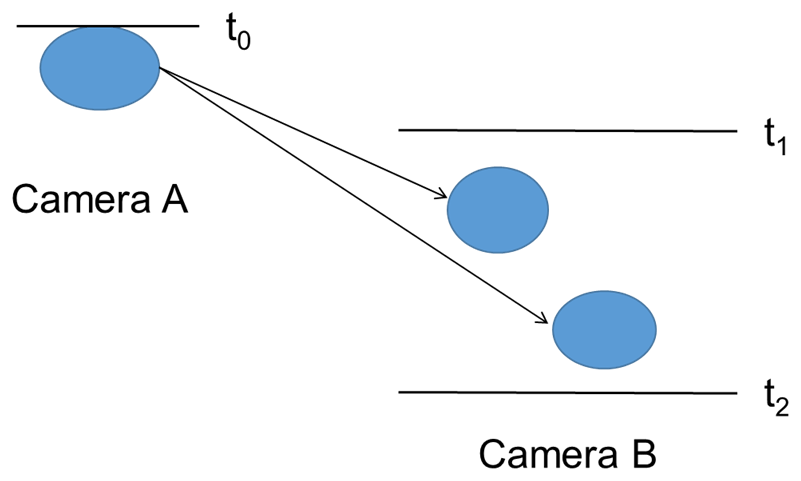
Figure 2 Illustration of the matching procedure. In the situation shown, it is assumed that camera A observed a particle at time t₀, and afterwards during a certain time period, t₁ to t₂, camera B observed two particles. The matching procedure decides which particle observed by camera B is the same particle observed by camera A.

For methods 2 and 3 in Sect. 3.3, we used the manufacturer's matching algorithm, which gives the contour data. To avoid overestimating mass due to mismatch, we need to filter out those particles with unreasonable fall speeds. The vertical dimension of the particle's image before match is expressed as a number of scan lines (i.e., how many scan lines are masked by the particle). After match (so v_t is known), the vertical pixel width is v_t∕f_s, where f_s is the scan frequency of a camera (∼55 kHz), and the vertical size of the particle is the vertical pixel width multiplied by the number of scan lines. Because two optical planes of the 2DVD are parallel, theoretically, the number of scan lines from cameras A and B should be the same. Considering the distance from the particle to the two cameras (projective effect of a camera), the digital error of a camera and particle rotation in two planes, the difference in the number of scan lines between two cameras may not always be the same but should be very close. Hanesch (1999) gave a set of matching criteria, the most important being the tolerance of the number of scan lines between the two cameras (see Table 1). To obtain reliable fall speeds, we examined all matched particles (given by the manufacturer's matching algorithm, numbering 507 833 for the event and marked as green in Fig. 3) and removed those particles which did not satisfy the Hanesch scan line criteria, resulting in 175 199 (34.5 %) of particles that did satisfy the match criteria (magenta marks in Fig. 3). We used the fall speeds of these filtered particles to compute their mass for both Böhm and Heymsfield–Westbrook methods, and then divided the mass by apparent volume ($=\mathit{\pi }{D}_{\mathrm{app}}^{\mathrm{3}}/\mathrm{6}$) to get the particle density. Since the maximum density of ice particles is around 0.9 g cm⁻³, we further remove particles with density larger than 1 g cm⁻³. After this two-step filtering, the particles we use for further analysis (numbering 128 063) are shown in Fig. 3 as blue points. The filtering will eliminate particles, which will reduce the liquid equivalent snow accumulation. Hence, the Pluvio gauge accumulation is used as an integral constraint, i.e., the concentration in each bin is increased by a constant factor to match the 2DVD accumulation to the Pluvio accumulation. This constraint is only used in methods 2 and 3 in Sect. 3.3.

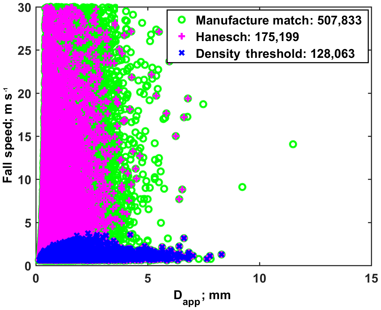
Figure 3 Fall speed vs. D_app for the synoptic case on 31 January 2012 at the CARE site. The green circles represent the results of the manufacturer's matching algorithm, which is known to allow mismatched particles with unrealistic fall speeds. The first filtering step is the selection of matched particles which satisfy Hanesch scan line criteria (magenta). The second filter step is shown as blue crosses, which are based on particles with density (from mass computed by Böhm's or Heymsfield–Westbrook method) lower than 1 g cm⁻³.

Table 1 Hanesch 2DVD scan line criteria.

2.3 Scattering model

The scattering computation of ice particles is difficult because of their irregular shapes with large natural variability (e.g., snow aggregates or rimed crystals). The most common scattering method used in the meteorological community is the discrete dipole approximation (DDA; Draine and Flatau, 1994). However, DDA is very time consuming and not suitable for large numbers of particles, especially at W-band (e.g., Chobanyan et al., 2015). On the other hand, the T-matrix method (Mishchenko et al., 2002) is more time efficient and commonly used in radar meteorology but it requires that the irregular particle shape be simplified to an axis-symmetric shape (e.g., spheroid). Ryzhkov et al. (1998) have shown that, in the Rayleigh region, the radar cross section is mainly related to particle's mass squared and less to the shape. For Mie scattering, however, the irregular snow shape plays a more significant role. Westbrook et al. (2006, 2008) used the Rayleigh–Gans approximation to develop an analytical equation for the scattering cross sections of simulated snow aggregates of bullet rosettes using an empirical fit to the form factor that accounts for deviations from the Rayleigh limit. Here, we use two scattering models, one based on the soft spheroid (Huang et al., 2015) with a fixed axis ratio and quasi-random orientation. The apparent density is calculated as the ratio of mass to apparent volume. There is considerable controversy in the literature on the applicability of the soft spheroid model with a fixed axis ratio, especially at Ka and higher frequencies such as W-band (e.g., Petty and Huang, 2010; Botta et al., 2010; Leinonen et al., 2012; Kneifel et al., 2015). However, Falconi et al. (2018) used the soft spheroid scattering model using T-matrix to compute Z_e (at X-, Ka-, and W-bands) and showed that an effective optimized axis ratio of (oblate) spheroid could be selected that directly matches measured Z_e by radar (their optimal axis ratio, however, varied with the frequency band, i.e., 1 for X-band, 0.8 for Ka, and 0.6 for W). They also found some differences in the optimal axis ratios for fluffy snow vs. rimed snow. Nevertheless, they compared DDA calculations of complex-shaped aggregates to the soft spheroid model at W-band and concluded that the axis ratio can be used as a tuning parameter. They also showed the importance of size integration to compute Z_e, i.e., the product of N(D) and the radar cross section for the soft spheroid vs. complex-shape aggregates. Their result implied that smaller particles had a larger value for the product when using a soft spheroid of 0.6 axis ratio relative to complex aggregates and vice versa for larger particles, leading to compensation when Z_e is computed by size integration over all sizes. Thus, the soft spheroid model with axis ratio at 0.8 used by Huang et al. (2015), and which is used herein at Ku- and Ka-bands, is a reasonable approximation.

The second scattering model we used herein is from Liao et al. (2013), who use an effective fixed density approach to justify the oblate spheroid model. To compare the scattering properties of a snow aggregate with its simplified equal-mass spheroid, Liao et al. (2013) used six-branch bullet rosette snow crystals with maximum dimensions of 200 and 400 µm as two basic elements that simulate snow aggregation. They computed the backscattering coefficient, extinction coefficient, and asymmetry factor for simulated snowflakes, using the DDA and for the corresponding spheres and spheroids with the same mass but density fixed at 0.2 or 0.3 g cm⁻³, and hence the apparent sphere volume equals the mass divided by the assumed fixed density. They showed that, when the frequency was lower than 35 GHz (Ka-band), the Mie scattering properties of spheres with a fixed density equal to 0.2 g cm⁻³ were in a good agreement with the scattering results for the simulated complex-shaped aggregate model with the same mass using the DDA (see also Kuo et al., 2016). They also showed this agreement with a spheroid model with a fixed axis ratio of 0.6 and random orientation. Here, we use the Liao et al. (2013) equivalent spheroid model with a fixed effective density of 0.2 g cm⁻³ at Ku- and Ka-bands (note that we estimate the mass of each particle from 2DVD measurements as described in Sect. 2.1). Note that this fixed-density spheroid scattering model is not based on microphysics (where the density would fall off inversely with increasing size) but on scattering equivalence with a simulated (same-mass) complex-shaped aggregate snowflake (Liao et al., 2016).

3 Case analysis

3.1 Test site instrumentation and the synoptic event

The GPM Cold-season Precipitation Experiment (GCPEx) was conducted by the National Aeronautics and Space Administration (NASA), USA, in cooperation with Environment Canada in Ontario, Canada from 17 January to 29 February 2012. The goal of GCPEx was “… to characterize the ability of multi-frequency active and passive microwave sensors to detect and estimate falling snow…” (Skofronick-Jackson et al., 2015). The field experiment sites were located north of Toronto, Canada between Lake Huron and Lake Ontario. The GCPEx had five test sites, namely CARE (Centre for Atmospheric Research Experiments), Sky Dive, Steam Show, Bob Morton, and Huronia. The locations of five sites are shown in Fig. 4. The CARE site was the main test site for the experiment, located at 44^∘13^′58.44^′′ N, 79^∘46^′53.28^′′ W and equipped with an extensive suite of ground instruments. The 2DVD (SN37) and OTT Pluvio² 400 used for observations and analyses in this paper were installed inside a DFIR (double fence intercomparison reference) wind shield. The dual-frequency dual-polarized doppler radar (D3R) was also located at the CARE site (Vega et al., 2014) near the 2DVD. The instruments used in this paper are depicted in Fig. 5. Because the radar and the instrumented site were nearly collocated, we can effectively view the set-up as similar to a vertical-pointing radar as described in more detail in Sect. 3.2.

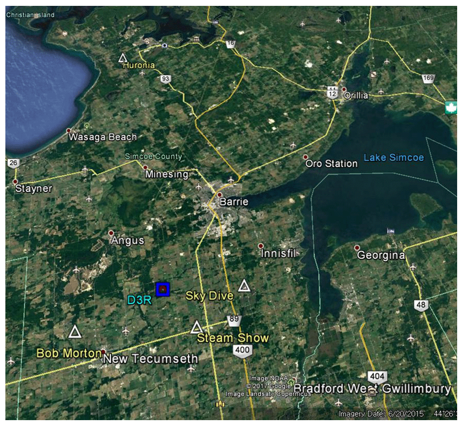
Figure 4 A map of the GCPEx field campaign. The five test sites are CARE, Sky Dive, Steam Show, Bob Morton, and Huronia. The ground observation instruments, namely 2DVD, D3R, and Pluvio, used in this research, were located at CARE.

Figure 5 Instruments used in this study: (a) 2DVD (SN37), (b) D3R (dual-wavelength dual-polarized doppler radar), and (c) OTT Pluvio² 400 precipitation gauge.

We examine a snowfall event on 30–31 January 2012 that occurred across the GCPEx study area between roughly 22:00 UTC, 30 January and 04:00 UTC, 31 January. Details of this case using King City radar and aircraft spiral descent over the CARE site is given in Skofronick-Jackson et al. (2015). This event resulted in liquid accumulations of roughly 1–4 mm across the GCPEx domain with fairly uniform snowfall rates throughout the event. At the CARE site the accumulations over an 8 h period were <3.5 mm. Echo tops as measured by high-altitude airborne radar were 7–8 km. The precipitation was driven by a shortwave trough moving from southwest to northeast across the domain. Figure 6 displays the 850 hPa geopotential heights (m), temperature (K), relative humidity (%), and winds (m s⁻¹) at 00:00 UTC, 31 January, during the middle of the accumulating snowfall. A trough axis is apparent just to the west of the GCPEx domain (green star in Fig. 6). Low-level warm-air advection forcing upward motion is coincident with high relative humidity on the leading edge of the trough, over the GCPEx domain (Fig. 6). Temperatures in this layer were around −10 to −15 ^∘C throughout the event, supporting efficient crystal growth, aggregation, and potentially less dense snowfall as this is in the dendritic crystal temperature zone (e.g., Magono and Lee, 1966). Aircraft probe data during a descent over the CARE site between 23:15 and 23:43 UTC showed the median volume diameter (D₀) of 3 mm, with particles up to a maximum of 8 mm (aggregates of dendrites) at 2.2 km m.s.l. with a large concentration of smaller sizes < 0.5 mm (dendritic and irregular shapes; Skofronick-Jackson et al., 2015). At the surface, photographs of the precipitation types by the University of Manitoba showed small irregular particles and aggregates (<3 mm) at 23:30 UTC on 30 January.

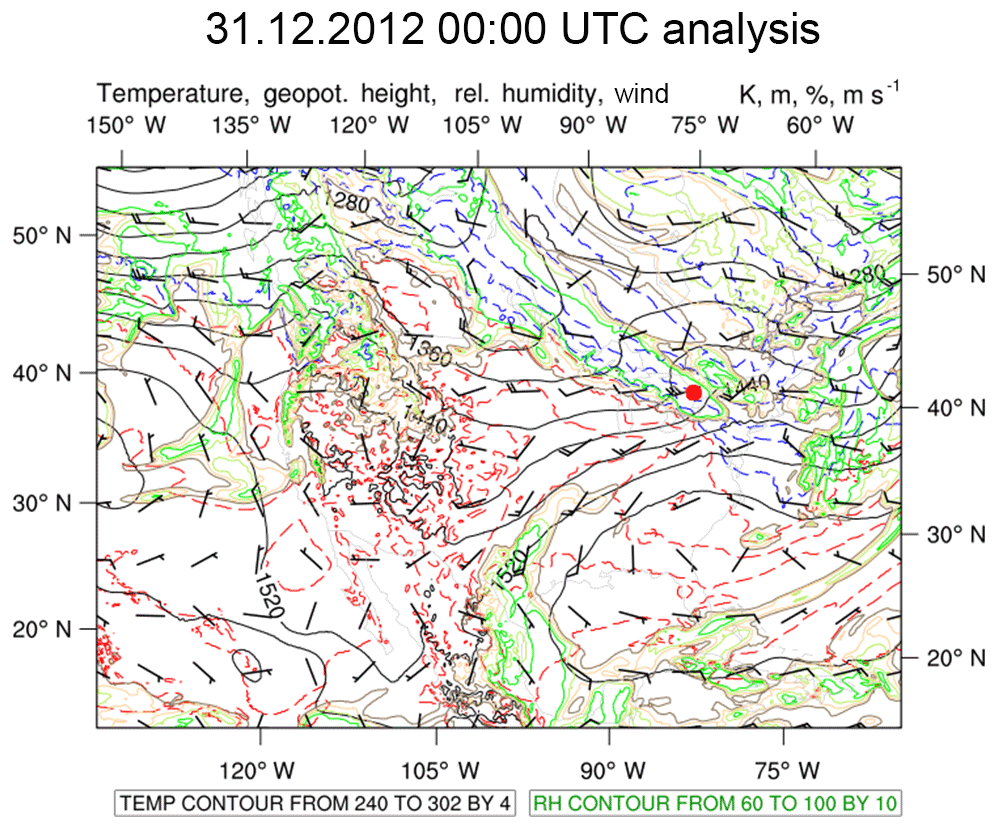
Figure 6 The 00:00 UTC, 31 January 2012, 850 hPa geopotential heights (m, black solid contours), temperature (K, red: above freezing, blue: below freezing), relative humidity (%, green shaded contours), and wind (m s⁻¹, wind barbs). The red dot in the center right portion of the figure denotes the general location of the GCPEx field instruments.

3.2 D3R radar data

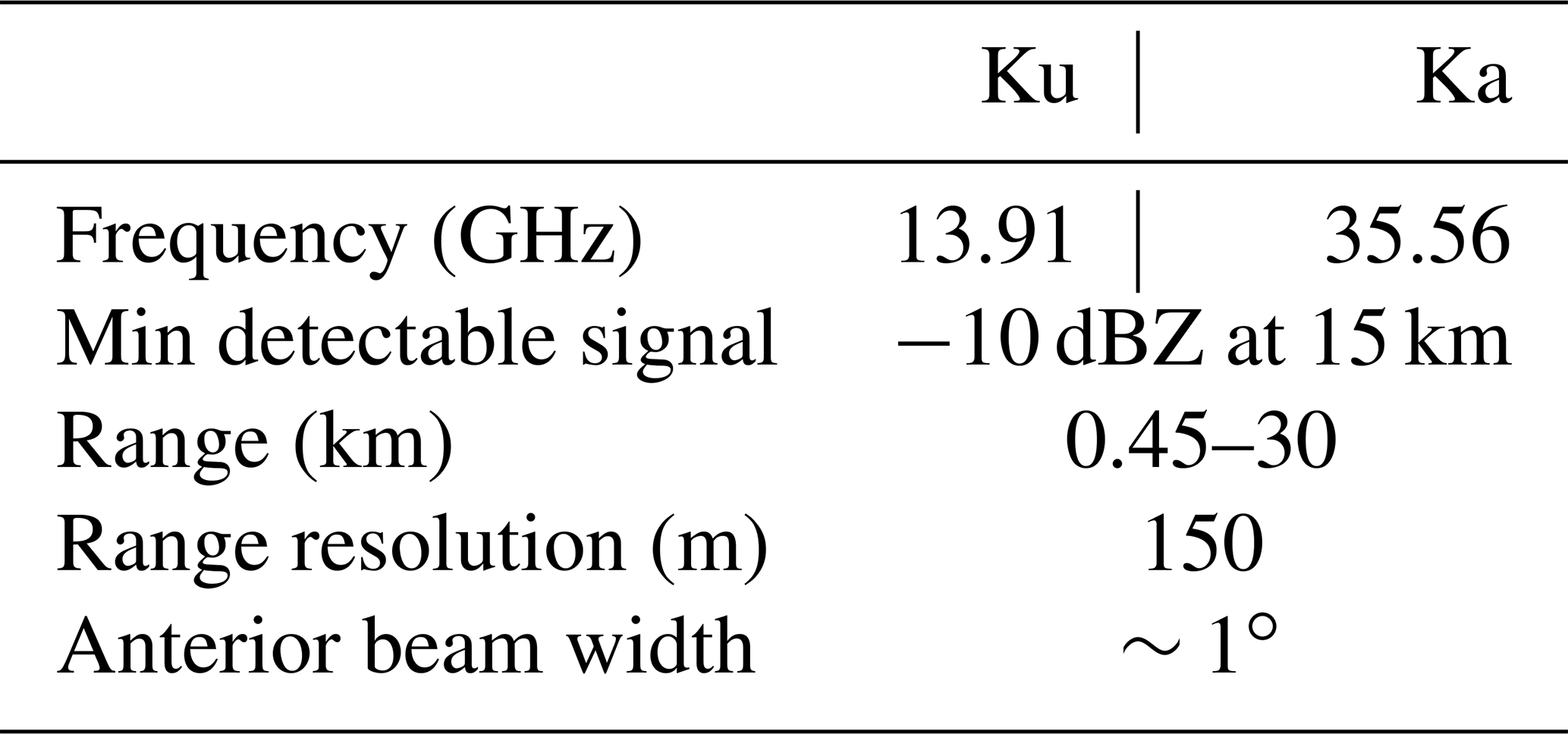
The D3R is a Ku- and Ka-band dual-wavelength polarimetric scanning radar. It was designed for ground validation of rain and falling snow from GPM satellite-borne DPR (dual-frequency precipitation radar). The two frequencies used in the D3R are 13.91 GHz (Ku) and 35.56 GHz (Ka). These two frequencies were used for scattering computations in this research as well. Some parameters of the D3R radar relevant for this paper are shown in Table 2. The range resolution of the radar is adjustable but usually set to 150 m and the near-field distance is ∼300 m; the practical minimum operational range is around 450 m. The minimum detectable signal of the D3R is −10 dBZ at 15 km. This means that when Z_h is −10 dBZ at 15 km, the signal-to-noise ratio (SNR) is 0 dB. Therefore, the SNR at any range, r, can be computed as follows:

$$\begin{array}{}\text{(1)}& \text{SNR}\left(r\right)=Z_{\mathrm{h}}\left(r\right)+\mathrm{10}+\mathrm{20}{\log }_{\mathrm{10}}\left({\displaystyle \frac{\mathrm{15}}{r}}\right)\left[\mathrm{dB}\right].\end{array}$$

The SNR is a very important indicator for radar data quality control (QC), the other important parameter for QC (in terms of detecting “meteo” vs. “nonmeteo” echoes) being the texture of the standard deviation (SD) of the differential propagation phase (φ_dp). We randomly selected 20 out of 85 RHI sweeps from 31 January 2012 and computed the SD of Ku-band φ_dp for each beam over 10 consecutive gates where SNR ≥10 dB. According to the histogram of the SD of φ_dp, 90 % of the values were less than around 8^∘. Radar data at a range gate m are identified as “good” data (i.e., meteorological echoes) only if the standard deviation of φ_dp from the (m−5)th gate to the (m+4)th gate is less than 8^∘. This criterion sets a good data mask for each beam at Ku-band. On the other hand, the φ_dp at Ka-band was determined to be too noisy and hence not used herein. The good data mask for the Ka-band beam is set by the mask determined by the Ku-band criteria, with the additional requirement that the Ka-band SNR >3 dB for the range gate to be considered good. Note that both radars are mounted on a common pedestal so that the Ku and Ka-band beams are perfectly aligned.

Table 2 Some D3R parameters relevant for this study. Full D3R specifications can be found in Vega et al. (2014).

There are four scan types that can be performed by the D3R, namely PPI (plan position indicator), RHI (range height indicator), surveillance, and vertical pointing. Figure 7 shows the scan strategies of the D3R on 31 January 2012, which consisted of a fast PPI scan (surveillance scan; 10^∘ per second) followed by four RHI scans (1^∘ per second), except from 01:00 to 02:00 UTC. The RHI scans with an azimuth angle of 139.9^∘ point to the Steam Show site and those at 87.8^∘ point to the Sky Dive site. There were no RHI scans pointing to the Bob Morton site, and Huronia (52 km) was beyond the operational range (maximum 30 km) of the D3R. During the most intense snowfall the D3R scans did not cover the instrument clusters at the Sky Dive and Steam Show sites. So we were left with the analysis of the D3R radar data at close proximity to the 2DVD or effectively vertical-pointing equivalent using RHI data from 75 to 90^∘ at the nearest practical range of 600 m. PPI scan data at low elevation angle (3^∘) were also used from range gate at 600 m. The assumption is that there is little evolution of particle microphysics from about 600 m height to the surface and that the synoptic-scale snowfall was uniform in azimuth (confirmed by Skofronick-Jackson et al., 2015). The snowfall was spatially uniform around the CARE site so we selected data at 600 m range to be compared with the 2DVD and Pluvio observations (this range was selected based on the minimum operational range of 450 m; see Table 2) to which 150 m was added based on close examination of data quality. For RHI scans, the Z_h at each band was averaged over the beams from 75 to 90^∘. The 75^∘ is obtained from $\mathrm{600}\cdot \cos \left(\mathrm{75}{}^{\circ }\right)\approx \mathrm{155}$ m which is close to the range resolution. For the fast PPI scan, Z_h was averaged over all azimuthal beams at 600 m range.

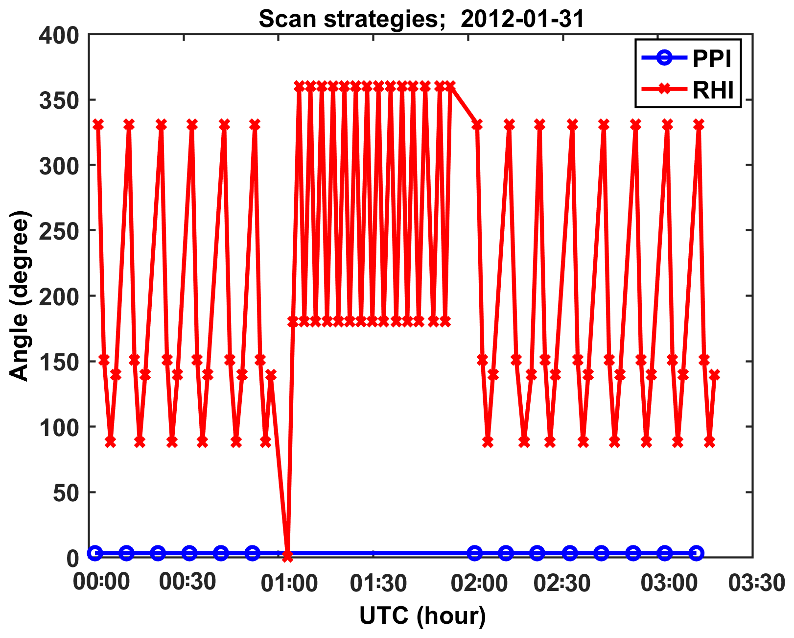
Figure 7 D3R scan strategies on 31 January 2012. The y axis is azimuth angle (RHI; red x) or elevation angle (PPI; blue o). The scan rate of RHI was 1${}^{\circ }{\mathrm{s}}^{-\mathrm{1}}$ and 10${}^{\circ }{\mathrm{s}}^{-\mathrm{1}}$ for PPI.

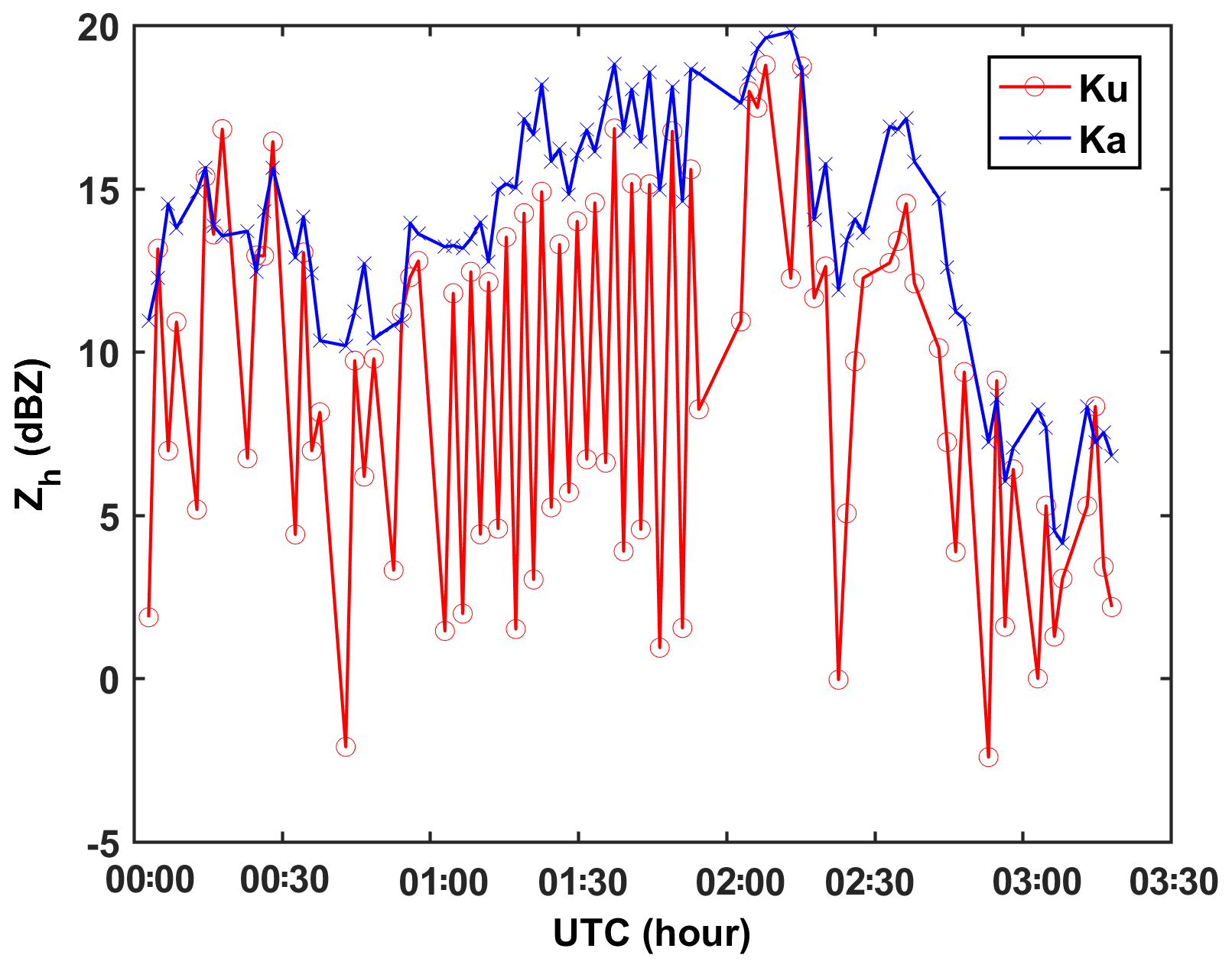
Figure 8 The time series of averaged raw Z_h at the CARE site. There are two problems indicated in this figure: (i) the Ku-band Z_h is smaller than the Ka-band Z_h on average. (ii) Compared with the Ka-band, there are many too small values of the Ku-band Z_h.

Figure 8 shows the time profile of the averaged Z_e at Ku- and Ka-bands. There are two problems indicated in this figure. First, theoretically, the Ku-band Z_e should be greater than or equal to the Ka-band Z_e. The smaller Ku-band Z_h indicates that a Z offset exists at both bands. The other problem is that, compared with the Ka-band, there are many dips in the Ku-band Z_h. By comparing Fig. 8 with Fig. 7, we found that these dips occur only at RHI scans with azimuth angle larger than 300^∘. We examined those RHI scans beam by beam from 90 to 75^∘. We further found that when the elevation angle is smaller than 78^∘, the unreasonably low Z_h disappears. Therefore, the RHI scans with azimuth angles larger than 300^∘ were averaged over the 75 to 78^∘ elevation angles. To compute the DWR, we need to know the Z offset between the two bands. The measured Z_h includes three components (neglecting attenuation):

$$\begin{array}{}\text{(2)}& Z_{\mathrm{h}}^{\mathrm{meas}}=Z_{\mathrm{h}}^{\mathrm{true}}\pm \text{error}\left(Z_{\mathrm{h}}\right)+Z_{\mathrm{offset}},\end{array}$$

where “error” refers to measurement fluctuations (typically with standard deviation of ∼1 dB). The DWR is obtained as the difference between Ku-band Z_h and Ka-band Z_h, with Z_h being in units of dBZ. The measured DWR is as follows:

$$\begin{array}{}\text{(3)}& {\text{DWR}}^{\mathrm{meas}}={\text{DWR}}^{\mathrm{true}}\mp \text{error}\left(\text{DWR}\right)+\mathrm{\Delta }{Z}_{\mathrm{offset}},\end{array}$$

where error (DWR) is now increased, since the Ku- and Ka-band measurement fluctuations are uncorrelated (standard deviation of around 1.4 dB). The ΔZ_offset is determined by selecting data where the scatterers (snow particles) are sufficiently small in size so that Rayleigh scattering is satisfied at both bands, i.e., DWR^true=0 dB. The criteria are used here to select gates where Ku-band Z_h<0 dBZ along with spatial averaging, which reduces the measurement fluctuations in DWR to estimate ΔZ_offset in Eq. (3). Figure 9 shows the averaged Z_h for the two bands from 20 RHI scans which satisfy the conditions above. After removing three extreme values (outliers) from Fig. 9, ΔZ_offset was estimated as −1.5 dB, which is used in the subsequent data processing.

Figure 9 The averaged raw Z_h for Ku- and Ka-bands. The Z_h was randomly selected from 20 of 85 RHI scans with Ku-band Z_h<0 dBZ, range <1 km, and Ka-band SNR >3 dB.

3.3 2DVD data analysis

The 2DVD used in this study was also located at the CARE site. The particle-by-particle mass estimation is based on three methods as follows:

1. Following the procedure in Huang et al. (2015) we use 2DVD single-camera data and apply the weighted Hanesch-matching algorithm (Hanesch, 1999) to rematch snowflakes. A PSD adjustment factor is computed as in Huang et al. (2015) without using the Pluvio gauge as a constraint. Mass is computed from fall speed, D_app and environmental conditions using Böhm (1989). The apparent density of the snow (ρ) is defined as $\mathrm{6}m/\mathit{\pi }{D}_{\mathrm{app}}^{\mathrm{3}}$. A mean power-law relation of the form $\mathit{\rho }=\mathit{\alpha }{D}_{\mathrm{app}}^{\mathit{\beta }}$ is derived for the entire event as in Huang et al. (2015) as well as 1 min averaged N(D_app) is calculated. Note that the scattering model is based on the soft spheroid model with fixed axis ratio =0.8 and apparent density ρ. The results obtained by this method are denoted HB in the figures and in the rest of the paper.

2. Use the manufacturer's (Joanneum Research, Graz, Austria) matching algorithm and filter-mismatched snowflakes as described in Sect. 2.2. The mass is computed from Böhm's equations. The PSD adjustment factor is based on using the Pluvio gauge accumulation as a constraint. Following Liao et al. (2013) as far as the scattering model is concerned, the density is fixed at 0.2 g cc⁻¹ and the volume is computed from $\text{mass}=\text{density}\cdot \text{volume}$. The effective equal-volume diameter is D_eff and the corresponding PSD is denoted N(D_eff), which is different from N(D_app) in (1) above. Henceforth, this method is denoted LM.

3. Use Joanneum matching and filtering method as in (2) but compute mass using Heymsfield–Westbrook equations as well as the revised D_eff and N(D_eff). This method is denoted HW. Thus, the only difference with (2) is in the estimation of mass and the difference in D_eff and N(D_eff). The PSD adjustment factor is based on using the Pluvio gauge accumulation as a constraint. The scattering model follows Liao et al. (2013).

The 2DVD measured liquid equivalent snow rate (SR) can be computed directly from mass as follows:

$$\begin{array}{}\text{(4)}& \text{SR}={\displaystyle \frac{\mathrm{3600}}{\mathrm{\Delta }t}}\sum _{i=\mathrm{1}}^N\sum _{j=\mathrm{1}}^M{\displaystyle \frac{V_j}{A_j}};\left[\mathrm{mm}{\mathrm{h}}^{-\mathrm{1}}\right],\end{array}$$

where Δt is the integral time (typically 60 s), N is the number of size bins (typically 101 for the 2DVD), M is the number of snowflakes in the ith size bin, and A_j is the measured area of the jth snowflake. Further, V_j is the liquid equivalent volume of the jth snowflake, so it is directly related to the mass. Figure 10 compares the liquid equivalent accumulation computed using the three methods above based on 2DVD measurements with the accumulation directly measured by the collocated Pluvio snow gauge. The Pluvio-based accumulation at the end of the event (03:30 Z) was 1.9 mm while the 2DVD-measured accumulations using the three methods are 1.27 mm (HB), 1.45 mm (LM), and 1.24 mm (HW). It is expected that the PSDs of LM and HW should be underestimated because of eliminating mismatched particles which, in principle, could be rematched. Rematching mismatched particles is a research topic on its own and is beyond the scope of this paper. We used a simple way to adjust the PSD for methods 2 and 3 by scaling the PSD by a constant so that the final accumulation matches the Pluvio gauge accumulation. Specifically, the PSD adjustment factors are 1.3 for LM and 1.52 for HW. Note that PSD adjustment of HB (method 1) is not done by forcing 2DVD accumulation to agree with Pluvio, rather the method described in Huang et al. (2015) is used giving the adjustment factor of 1.54 for 00:00–00:45 UTC and 1.11 for 00:45–04:00 UTC. From the Pluvio accumulation data in Fig. 10 the SR is nearly constant at 0.7 mm h⁻¹ between relative times of 1.5 and 3 h (or actual time from 01:00 on 30 January to 02:30 UTC).

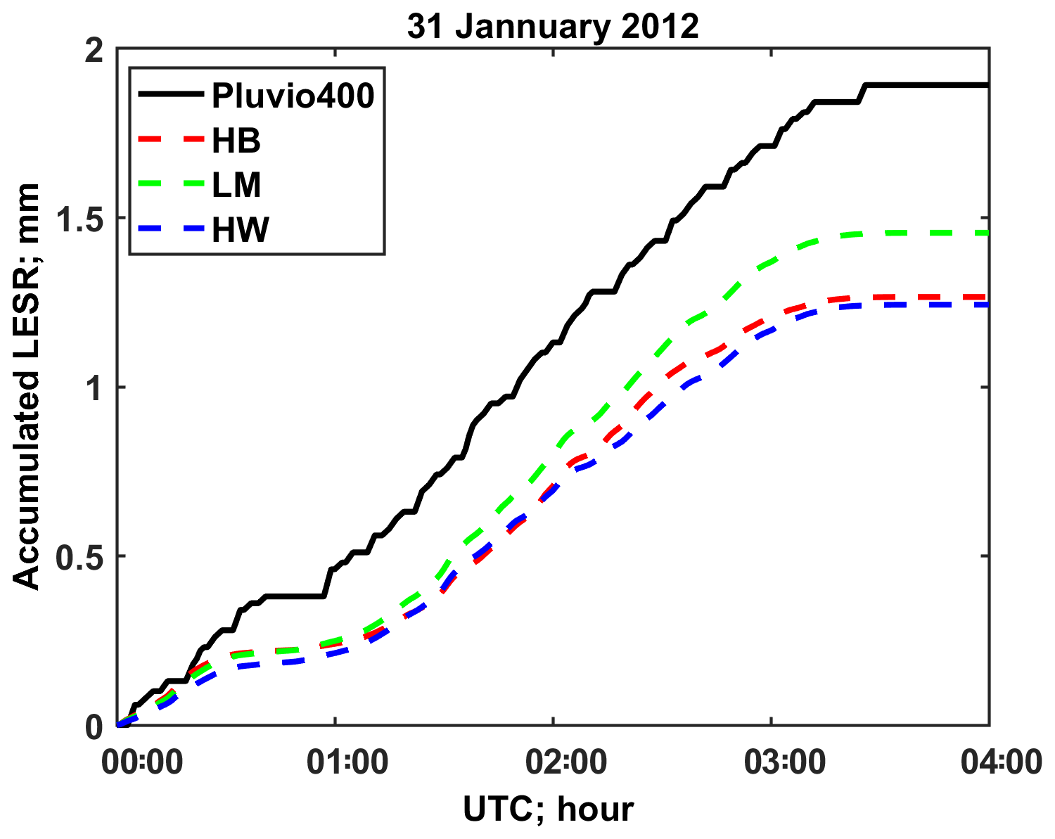
Figure 10 Comparison of liquid equivalent accumulations computed using HB, LM, and HW methods based on 2DVD measurements and that were directly measured by the collocated Pluvio snow gauge. We used the total accumulation to estimate the PSD adjustment factor for the LM and HW methods.

The radar reflectivities at the two bands are simulated by using the T-matrix method assuming a spheroid shape with an axis ratio of 0.8, consistently with Falconi et al. (2018). The PSD is adjusted for methods 1, 2, and 3 as described above. The orientation angle distribution is assumed to be quasi-random with Gaussian distribution for the zenith angle $[\text{mean}=\mathrm{0}{}^{\circ },\mathit{\sigma }=\mathrm{45}{}^{\circ }]$ and uniform distribution for the azimuth angle. However, other studies have assumed $\mathit{\sigma }=\mathrm{10}{}^{\circ }$ (Falconi et al., 2018). The recent observations of snowflake orientation by Garrett et al. (2015) indicate that substantial broadening of the snow orientation distribution can occur due to turbulence. Figure 11 compares the time series of D3R-measured Z_h with the 2DVD-derived Z_e for the entire event (20:00–03:30 UTC at (a) Ku- and (b) Ka-band). The Z_e for both bands computed by the three methods generally agree with the D3R measurements to within 3–4 dB. Overall, LM gives the highest Z_e and HB gives the lowest, which is especially evident at Ka-band. This is consistent with scattering calculations by Kuo et al. (2016) of single spherical snow aggregates using constant density (0.3 g cc⁻¹) giving higher radar cross sections and size-dependent density, i.e., density falls off as inverse size (giving lower cross sections). This feature is consistent with the scattering models referred to herein as LM and HB.

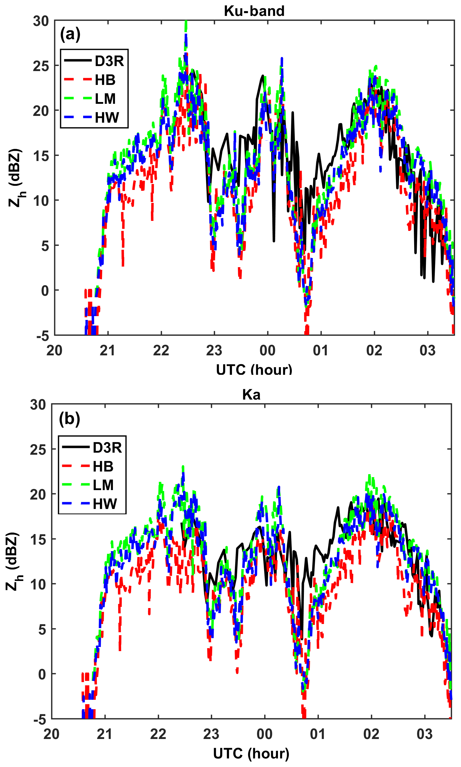
Figure 11 Comparison of the 2DVD-derived Z_h with D3R measurements for the entire event, Ku-band (a), and Ka-band (b). This synoptic system started at around 21:00 Z on 30 January and ended at around 03:30 Z on 31 January 2012. Z_e by LM is close to HW and slightly higher, whereas the HB method gives the lowest Z_e. Z_e results computed by all methods generally agree with D3R measured Z_h.

From 00:45 to 01:30 UTC on 31 January 2012, the three 2DVD-derived Z_e simulations deviate systematically from the D3R results for both bands. The other period is from 23:00 to 23:30 UTC on 30 January 2012, when the Ku-band Z_e has significant deviation from the D3R observations but the Ka-band Z_e generally agrees with the D3R. Note that this synoptic event started at around 21:00 UTC on 30 January and stopped at 03:30 UTC. We checked the D3R data and found that, before 22:30 UTC, the RHI scans were from 0 to 60^∘, so there were no usable data available for comparison with the 2DVD and Pluvio at the CARE site. We note that at 00:30 UTC the King City C-band radar recorded Z_h in the range 15–20 dBZ around the CARE site, which is in reasonable agreement with the D3R radar observations (Skofronick-Jackson et al., 2015).

Figure 12a compares the time series of DWR simulated from 2DVD observations with the D3R measurements, whereas Fig. 12b shows the scatterplot In general, HB appears in qualitatively better agreement (better correlated and with significantly less bias) with D3R measurements relative to both LM and HW (significant underestimation relative to D3R). The scatterplot in Fig. 12b is an important result since in the HB method the soft spheroid scattering model is used with density varying approximately inverse with D_app (density-D_app power law where the larger snow particles have lower density). Hence for a given mass the D_app is larger (relative to Ka-band wavelength) and enters the Mie regime, which lowers the radar cross section at Ka-band (relative to same mass but constant density radar cross section in LM and HW). Whereas at Ku-band the difference in radar cross sections is less between the two methods (Rayleigh regime). The significant DWR bias in LM and HW relative to DWR observations is somewhat puzzling in that the Liao et al. (2013) scattering model radar cross sections agree with the synthetic complex shaped snow aggregates of the same mass at Ka-band, whereas the HB model underestimates the radar cross section relative to the synthetic complex shaped aggregates. On the other hand, Falconi et al. (2018) demonstrate that the soft spheroid model is adequate at X (close to Ku-band) and Ka-band and by inference adequate for DWR calculations with the caveat that different effective axis ratios may need to be used at Ka- and W-bands.

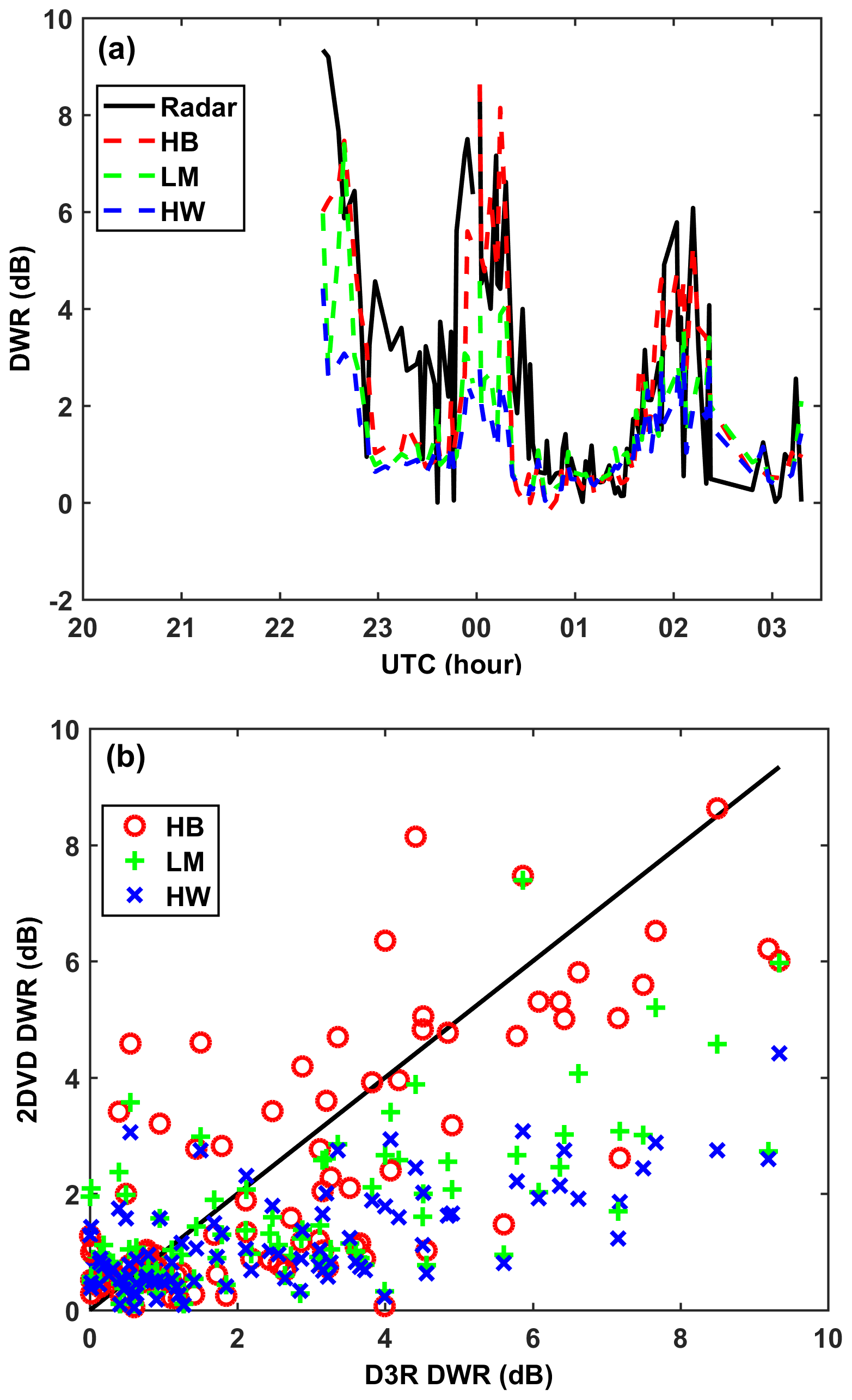
Figure 12 Comparison of the 2DVD-derived DWR using HB, LM, and HW methods with the D3R-measured DWR. Panel (a) shows the time profile of the D3R, and (b) shows the scatterplot.

We also refer to airborne (Ku, Ka) band radar data at 00:30 UTC which showed DWR measurements of 3–6 dB about 1 km height MSL around the CARE site but nearly 0 dB above that all the way to the echo top (Skofronick-Jackson et al., 2015). The latter is not consistent with aircraft spirals over the CARE site about an hour earlier where maximum snow sizes reach ∼8 mm. In spite of the difficulty in reconciling the observations from the different sensors, the appropriate scattering model in this particular event appears to favor the soft spheroid model used in HB based on better agreement with DWR observations. The other factor to be considered is the PSD adjustment factor, which is assumed constant and independent of size, which may not be the case, especially for the LM and HW methods as considerable filtering is involved due to mismatch (as discussed in Sect. 2.2). Note that a constant PSD adjustment factor will not affect DWR but it will affect Z_e. For the HB method Huang et al. (2015) determined the PSD adjustment factor for four events by comparing the 2DVD PSD to that measured by a collocated SVI (snow video imager which was assumed to be the “truth”) for each size bin. The PSD adjustment was found to not be size dependent for the HB method. On the other hand, because of the filtering of mismatched particles by the LM and HW methods, the PSD adjustment factor may be size dependent in which case the DWR will also change. More case studies are clearly needed to understand the applicability of the LM and HW methods of simulating DWR.

3.4 Snow rate estimation

To obtain radar–SR relationships, we use the 2DVD data and simulations. Since we employ a constant PSD adjustment factor, it will scale both Z_e and SR similarly. Figure 13 shows the scatterplot of the 2DVD-derived Z_e vs. 2DVD-measured SR along with a power-law fit as Z=aSR^b. The fitting method used is based on weighted total least square (WTLS) so the power law can be inverted without any change. The coefficients and exponents of the power-law Z–SR relationship for both bands and three methods are given in Table 3. It is obvious from Fig. 13 that there is considerable scatter at Ku-band for all three methods with the normalized standard deviation (NSD), ranging from 55 % to 70 %. Whereas at Ka-band the scatter is significantly lower with NSD from 40 % to 45 %. The errors in Table 3 are generally termed parameterization errors.

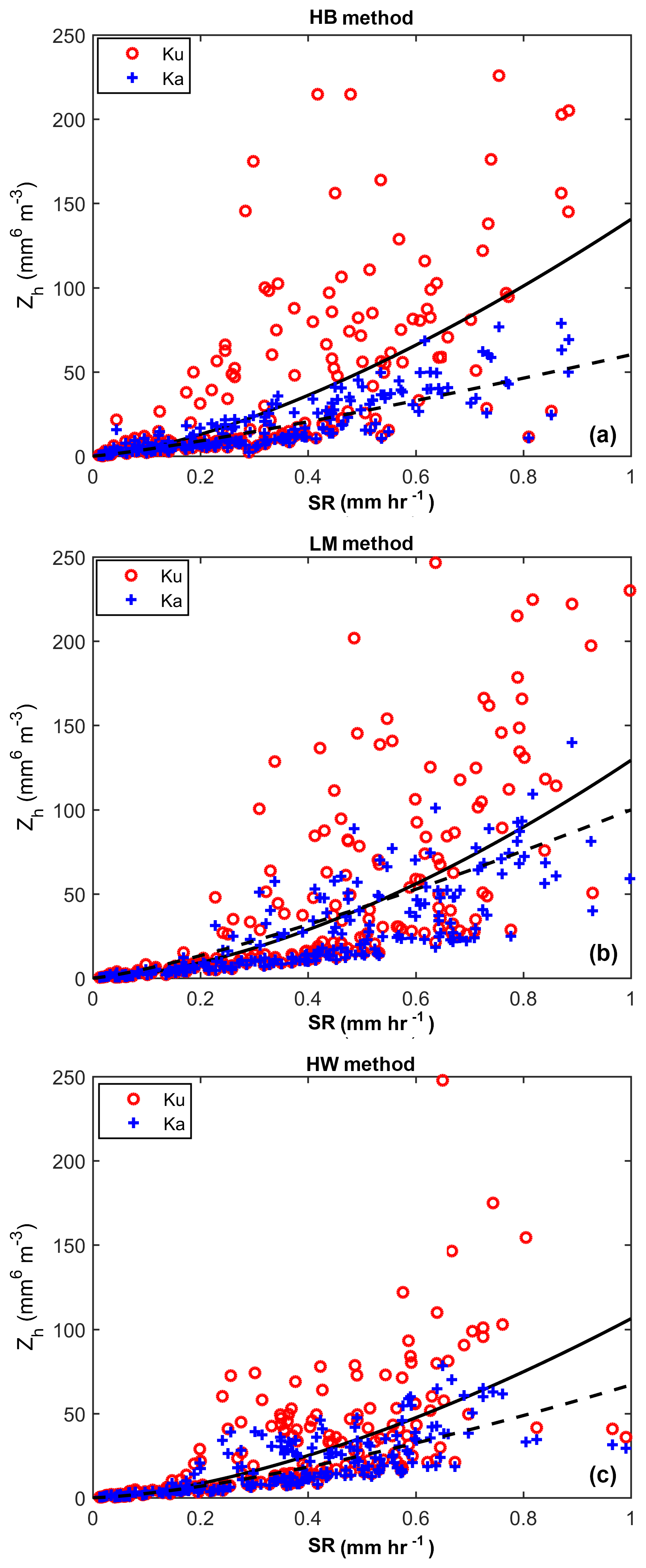
Figure 13 2DVD-derived Z_h vs. 2DVD-measured SR scatterplots, with Z–SR power-law fits, for Ku- and Ka-bands and the HB method (a), LM method (b), and HW method (c).

Table 3 Coefficients and exponents of the power-law Z–SR relationship for HB, LM, and HW methods and Ku- and Ka-bands, respectively.

By using dual-wavelength radar, we can estimate SR using Z_e at two bands as follows:

$$\begin{array}{}\text{(5)}& \left\{\begin{array}{c}{\text{SR}}_{\mathrm{Ku}}=a_{\mathrm{1}}^{\prime }\cdot Z_{\mathrm{Ku}}^{b_{\mathrm{1}}^{\prime }}\\ {\text{SR}}_{\mathrm{Ka}}=a_{\mathrm{2}}^{\prime }\cdot Z_{\mathrm{Ka}}^{b_{\mathrm{2}}^{\prime }}\end{array}\right.,\end{array}$$

where $a^{\prime }=(\mathrm{1}/a{)}^{b^{\prime }}$ and $b^{\prime }=\mathrm{1}/b$. To reduce error, we may take the geometric mean of these two estimators as follows:

$$\begin{array}{}\text{(6)}& \stackrel{\mathrm{‾}}{\text{SR}}={\left({\text{SR}}_{\mathrm{Ku}}\cdot {\text{SR}}_{\mathrm{Ka}}\right)}^{\mathrm{1}/\mathrm{2}}=c\cdot Z_{\mathrm{Ku}}^d\cdot {\text{DWR}}^e,\end{array}$$

where $c=(a_{\mathrm{1}}^{\prime }{a}_{\mathrm{2}}^{\prime }{)}^{\mathrm{1}/\mathrm{2}}$, $d=(b_{\mathrm{1}}^{\prime }+b_{\mathrm{2}}^{\prime })/\mathrm{2}$, and $e=-b_{\mathrm{2}}^{\prime }/\mathrm{2}$. Note that the DWR in Eq. (6) is on a linear scale, i.e., expressed as a ratio of reflectivity in units of mm⁶ m⁻³. Using Table 3 to set the initial guess of (c, d, e), nonlinear least squares fitting was used to determine the optimized (c, d, e) with the cost function being the squared difference between the 2DVD-based measurements of SR and $c{Z}_{\mathrm{Ku}}^d{\text{DWR}}^e$, where Z_Ku and DWR are from 2DVD simulations. Figure 14 shows the SR computed from the 2DVD simulations of Ku-band Z_e and the DWR using Eq. (6) vs. the 2DVD-measured SR. The (c, d, e) values for the three methods are given in Table 4. As can also be seen from Fig. 14 and Table 4, the SR(Z_Ku,DWR) using the LM method results in the lowest NSD of 28.49 %, but the other two methods have similar values of NSD (≈30 %) and, as such, these differences are not statistically significant. Although SR(Z_Ku,DWR) has a smaller parameterization error than Z_e–SR, the SR(Z_Ku,DWR) estimation is biased high when SR<0.2 mm h⁻¹ (see Fig. 14). When SR is small, the size of snowflakes is usually also small and falls in the Rayleigh region at both frequencies, resulting in DWR very close to 1 (when expressed as a ratio). This implies that there is no information content in the DWR so including it just adds to the measurement error. Hence, for small SR or when DWR ≈1, we use the Z_e–SR power law.

Table 4 Coefficients and exponents of the SR(Z_Ku,DWR) relation (see Eq. 10) for three methods.

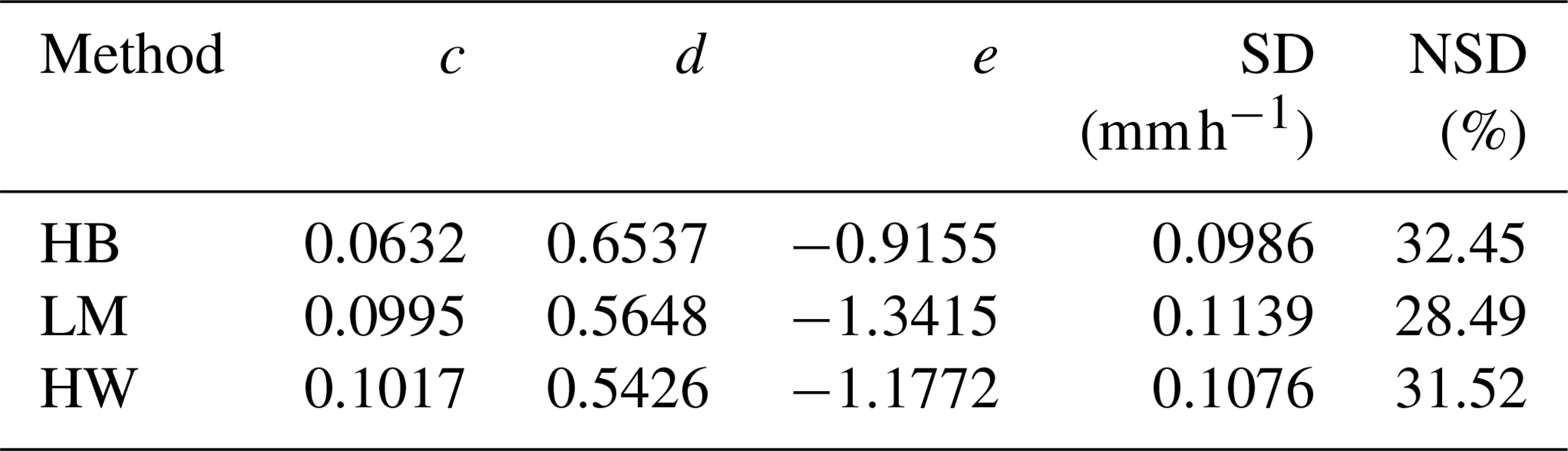
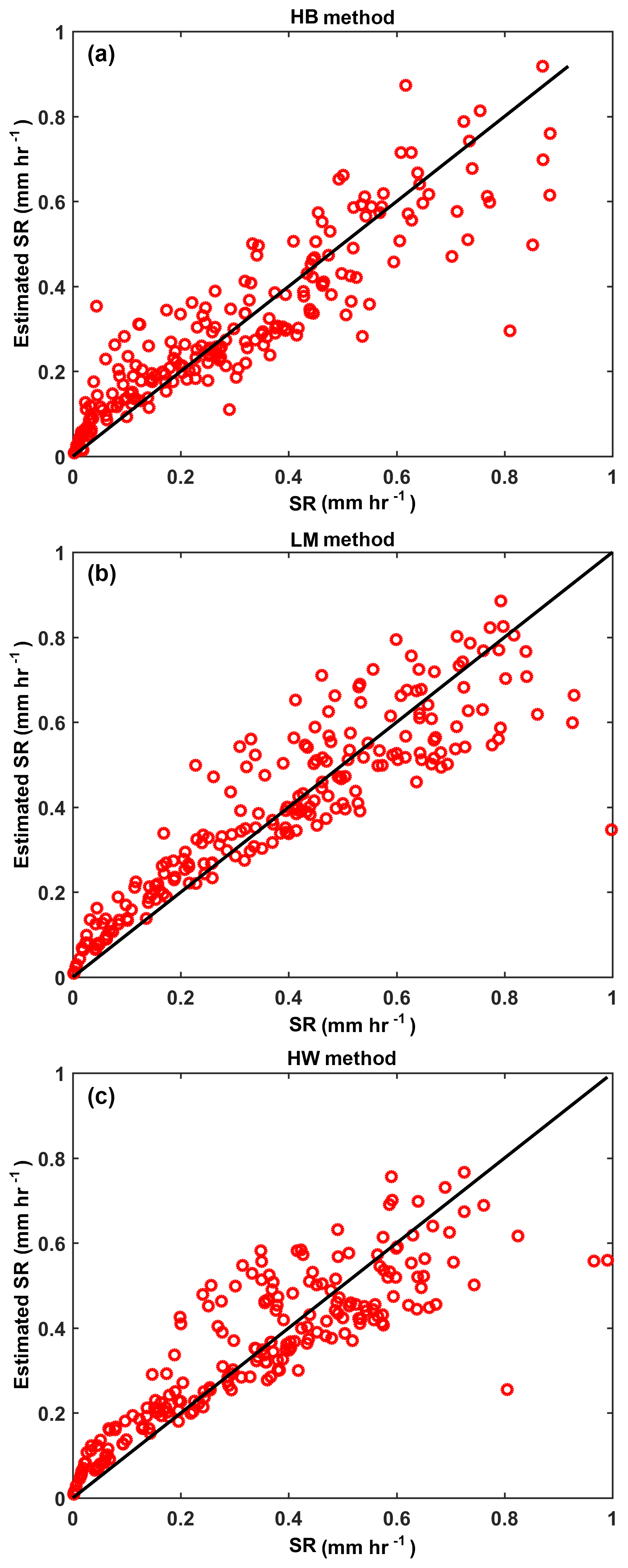
Figure 14 Estimated SR using Z_e and DWR of the 2DVD and Eq. (10) vs. 2DVD SR scatterplot for the HB method (a), LM method (b), and HW method (c).

So far the single-frequency SR retrieval algorithms were based on 2DVD-based simulations with a PSD adjustment factor using the total accumulation from Pluvio as a constraint. The algorithm we propose for radar-based estimation of SR is to use Eq. (6) when DWR >1 and SR >0.2 mm h⁻¹, else we use the Z_Ka–SR power law (note that we do not use the Z_Ku-SR power law as the measurement errors of Z_Ku seem to be on the high side, Fig. 9). The precise thresholds used herein are ad hoc and may need to be optimized using a much larger data set. Figure 15a shows the radar-derived accumulation using Z_Ka–SR vs. the Pluvio accumulation vs. time. The total accumulation from the Pluvio is 2.5 mm and the three radar-based total accumulations, for HB, LM, and HW methods amount to [2.6, 1.8, 2.6 mm]. Except for the underestimation in the LM method (−28 %), the other two methods agree with the Pluvio accumulation in this event. Figure 15b is the same as Fig. 15a, except the combination algorithm mentioned above is used. For this case, ∼33 % of data used the Z_Ka–SR power law due to threshold constraints given above. The event accumulations for HB, LM, and HW methods amount to [2.4, 1.9, 2.2 mm], which are consistent with the algorithm that uses only the Z_Ka–SR power law. However, the criteria of relative bias error in the total accumulation (in events with low accumulations such as this one) are not necessarily an indication that the DWR-based algorithm is not adding value. Rather, the criteria should be snow rate intercomparison, which could not be done due to the low resolution (0.01 mm min⁻¹) of the Pluvio² 400 gauge along with the low event total accumulation of only 2.5 mm. A close qualitative examination of Fig. 15b shows that the HB method more closely “follows” the gauge accumulation relative to HB in time in Fig. 15a. In Fig. 15, the time grid is different for the radar-based data and the gauge data. It is common to linearly interpolate the gauge data to the radar sampling time and if this is done, the rms error for the HB method reduces from 0.1 mm (when using only the Z_Ka–SR power law) to 0.045 mm for the DWR algorithm, which constitutes a significant reduction by a factor of 2.

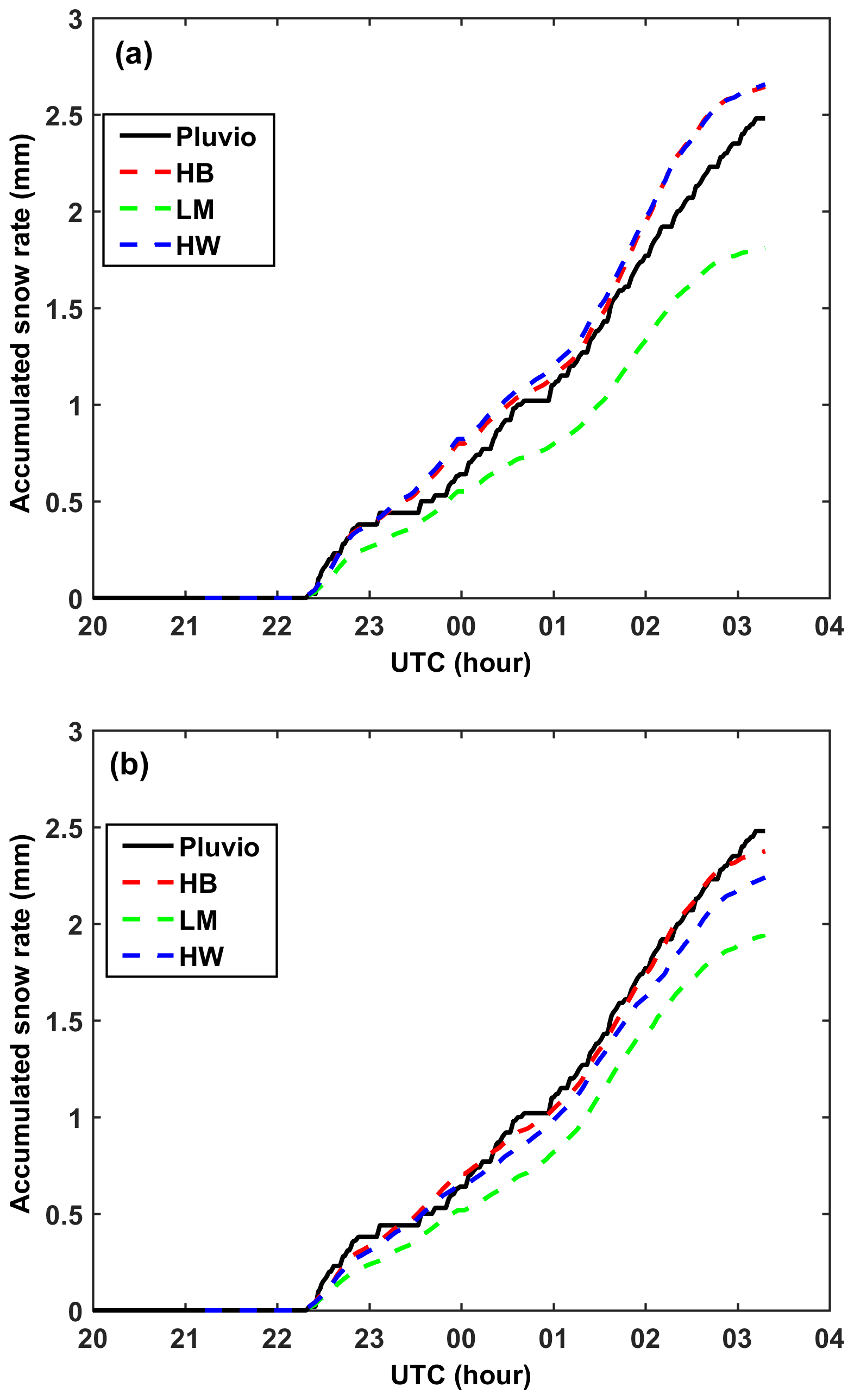
Figure 15 Comparison of the radar-derived accumulated SR using HB, LM, and HW methods with Pluvio gauge measurement. (a) The radar SR is computed by Z_Ka–SR relationships. The Pluvio-accumulated SR on 03:18 UTC is 2.48 mm. The radar-accumulated SRs for HB, LM, and HW are 2.64, 1.81, and 2.66 mm. (b) The radar SR is computed by combining SR(Z_Ku,DWR) and Z_Ka–SR as described in the text. The accumulated SR derived from the radar using HB method is 2.38 mm, using LM it is 1.94 mm and using HW it is 2.24 mm.

The total error in the radar estimate of SR is composed of both parameterization errors as well as measurement errors with measurement errors dominating, since the DWR involves the ratio of two uncorrelated variables. From Sect. 8.3 of Bringi and Chandrasekar (2001), the total error of SR in Eq. (6) is around 50 % (ratio of standard deviation to the mean). The assumptions are (a) the standard deviation of the measurement of Z_e is 0.8 dB, (b) the standard deviation of the DWR (in dB) measurement is 1.13 dB, and (c) the parameterization error is 30 % from Table 4. However, considering the Z_e fluctuations in Fig. 9, the measurement standard deviation probably exceeds 0.8 dB, especially at Ku-band. Thus, sufficient smoothing of DWR is needed to minimize the measurement error as much as possible while maintaining sufficient spatial resolution.

Note that the error model used here is additive with the parameterization, and measurement errors modeled as zero mean and uncorrelated with the corresponding error variances estimated either from data or via simulations (as described in Sect. 7 of Bringi and Chandrasekar, 2001). This is a simplified error model since it assumes that radar Z and snow gage measurements are unbiased based on accurate calibration. A more elaborate approach of quantifying uncertainty in precipitation rates is described by Kirstetter et al. (2015).

4 Summary and conclusions

The main objective of this paper is to develop a technique for snow estimation using scanning dual-wavelength radar operating at Ku- and Ka-bands (D3R radar operated by NASA). We use the 2-D video disdrometer and collocated Pluvio gauge to derive an algorithm to retrieve snow rate from reflectivity measurements at the two frequencies compared to the conventional single-frequency Z_e–SR power laws. The important microphysical information needed is provided by the 2DVD to estimate the mass of each particle knowing the fall speed, apparent volume, area ratio, and environmental factors from which an average density-size relation is derived (e.g., Huang et al., 2015; von Lerber et al., 2017; Böhm, 1989; Heymsfield and Westbrook, 2010).

We describe in detail the data processing of 2DVD camera images (in two orthogonal planes) and the role of particle mismatches that give erroneous fall speeds. We use the Huang et al. (2015) method of rematching using single-camera data but also use the manufacturer's matching code with substantial filtering of the mismatched particles since the apparent volume and diameter (D_app) are more accurate. To account for the filtering of the mismatched particles, the particle size distribution (in methods 2 and 3 in Sect. 3.3) is adjusted by a constant factor using the total accumulation from the Pluvio as a constraint.

Two scattering models are used to compute the Z_Ku and Z_Ka, termed the soft spheroid model (Huang et al., 2015; HB method) and the Liao–Meneghini (LM) model, which uses the concept of effective density. In these two methods the particle mass is based on Böhm (1989). The method of Heymsfield and Westbrook (2010) is also used to estimate mass which is similar to Böhm (1989) but is expected to be more accurate (Westbrook and Sephton, 2017); along with the LM model for scattering, this method is termed HW.

The case study chosen is a large-scale synoptic snow event that occurred over the instrumented site of CARE during GCPEx. The Z_Ku and Z_Ka were simulated based on 2DVD data and the three methods, i.e., HB, LM, and HW yielded similar values within ±3 dB. When compared with D3R radar measurements extracted as a time series over the instrumented site, the LM and HW methods were closer to the radar measurements with the HB method being lower by ≈3 dB. Some systematic deviations of simulated reflectivities by the three methods from the radar measurements were explained by a possible size dependence of the PSD adjustment factor.

The direct comparison of DWR (ratio of Z_Ku to Z_Ka) from simulations with DWR measured by radar showed that the HB method gave the lowest bias with the data points more or less evenly distributed along the 1:1 line. The simulation of DWR by LM and HW methods underestimated the radar measurements of DWR quite substantially, even though the correlation appeared to be reasonable. The reason for this discrepancy is difficult to explain since a constant PSD adjustment factor (different for method 1 relative to methods 2 and 3 in Sect. 3.3) would not affect the DWR. From the scattering model viewpoint, the LM method takes into account the complex shapes of snow aggregates via an effective density approach, whereas the HB method uses soft spheroid model with density varying approximately inversely with size. We did not attempt to classify the particle types in this study.

The retrieval of SR was formulated as $\text{SR}=c\cdot Z_{\mathrm{Ku}}^d\cdot {\text{DWR}}^e$, where [$c,d,e$] were obtained via nonlinear least squares for the three methods. The total accumulation from the three methods using radar-measured Z_Ku and DWR were compared with the total accumulation from the Pluvio (2.5 mm) to demonstrate closure. The closest to Pluvio was the HB method (2.4 mm), next was the HW method (2.24 mm) and then there was LM (1.94 mm). At such low total accumulations, the three methods show good agreement with each other as well as with the Pluvio gauge. The poor resolution of the gauge combined with the relatively low total accumulation in this event precluded direct comparison of snow rates. The combined estimate of parameterization and measurement errors for snow rate estimation was around 50 %. From variance decomposition, the measurement error variance as a fraction of the total error variance was 58 %, and the parameterization error variance fraction was 42 %. Further, the DWR was responsible for 90 % of the measurement error variance, which is not surprising since it is the ratio of two uncorrelated reflectivities. Thus, the DWR radar data have to be smoothed spatially (in range and azimuth) to reduce this error, which will degrade the spatial resolution but is not expected to pose a problem in large-scale synoptic snow events.

The snow rate estimation algorithms developed here are expected to be applicable to similar synoptic-forced snowfall under similar environmental conditions (e.g., temperature and relative humidity) but not, for example, to lake effect snowfall as the microphysics are quite different. However, analyses of more events are needed before any firm conclusions can be drawn as to applicability to other regions or environmental conditions.

Appendix A

Table A1 List of acronyms and symbols.