the Creative Commons Attribution 3.0 License.
the Creative Commons Attribution 3.0 License.
Application of the Fengyun 3 C GNSS occultation sounder for assessing the global ionospheric response to a magnetic storm event
Weihua Bai
Guojun Wang
Yueqiang Sun
Jiankui Shi
Guanglin Yang
Xiangguang Meng
Dongwei Wang
Qifei Du
Xianyi Wang
Junming Xia
Yuerong Cai
Congliang Liu
Wei Li
Chunjun Wu
Danyang Zhao
Di Wu
Cheng Liu
The rapid advancement of global navigation satellite system (GNSS) occultation technology in recent years has made it one of the most advanced space-based remote sensing technologies of the 21st century. GNSS radio occultation has many advantages, including all-weather operation, global coverage, high vertical resolution, high precision, long-term stability, and self-calibration. Data products from GNSS occultation sounding can greatly enhance ionospheric observations and contribute to space weather monitoring, forecasting, modeling, and research. In this study, GNSS occultation sounder (GNOS) results from a radio occultation sounding payload aboard the Fengyun 3 C (FY3-C) satellite were compared with ground-based ionosonde observations. Correlation coefficients for peak electron density (NmF2) derived from GNOS Global Position System (GPS) and Beidou navigation system (BDS) products with ionosonde data were higher than 0.9, and standard deviations were less than 20 %. Global ionospheric effects of the strong magnetic storm event in March 2015 were analyzed using GNOS results supported by ionosonde observations. The magnetic storm caused a significant disturbance in NmF2 level. Suppressed daytime and nighttime NmF2 levels indicated mainly negative storm conditions. In two longitude section zones of geomagnetic inclination between 40 and 80∘, the results of average NmF2 observed by GNOS and ground-based ionosondes showed the same basic trends during the geomagnetic storm and confirmed the negative effect of this storm event on the ionosphere. The analysis demonstrates the reliability of the GNSS radio occultation sounding instrument GNOS aboard the FY3-C satellite and confirms the utility of ionosphere products from GNOS for statistical and event-specific ionospheric physical analyses. Future FY3 series satellites and increasing numbers of Beidou navigation satellites will provide increasing GNOS occultation data on the ionosphere, which will contribute to ionosphere research and forecasting applications.
- Article
(1029 KB) - Full-text XML
- BibTeX
- EndNote


The Global navigation satellite system (GNSS) occultation technique uses occultation receivers mounted on low earth orbit (LEO) satellites to collect GNSS signals that are refracted and delayed by the atmosphere and ionosphere. The excess phase due to the atmosphere and ionosphere is determined from measurements of the delayed carrier phase and the precise positions and velocities of the LEO and GNSS satellites. An inverse Abel transform method is used to derive electron density of the ionosphere, the refraction index, temperature, humidity, and atmospheric pressure data, as shown in Fig. 1.

Figure 1Sketch of GNSS radio occultation sounding technology (using China's FY3-C satellite as an example).
GNSS radio occultation technology makes global-scale measurements of the atmosphere and ionosphere possible. It has the advantages of high precision, high vertical resolution, long-term stability, global coverage, all-weather operation, and a relatively low cost, which can compensate for some of the shortcomings of conventional atmospheric and ionospheric sounding tools (e.g., Fu et al., 2007). The global-scale data obtained have important scientific potential for improving the accuracy of numerical weather prediction, near-space environment monitoring research, global climate change research, atmospheric modeling research, and data assimilation. Radio occultation technology has significant scientific value and a broad array of potential practical applications in climatology, meteorology, ionospheric studies, and geodesy.
Radio occultation is extremely useful and important in ionosphere research, monitoring ionospheric anomalies, investigating ionospheric scintillation, and forecasting space weather. It also has a broad range of potential applications in communications, space operations, and national defense. Zhao et al. (2013) used ionosonde and radio occultation data to analyze differences in the ionosphere in eastern and western China, including the origins of ionospheric changes and latitudinal and longitudinal changes in structural layers of the ionosphere. Liu et al. (2008, 2009, 2010, 2011) used COSMIC radio occultation data to study seasonal changes in the electron density of the ionosphere, characteristics of the low-latitude ionosphere, and the scale height of the ionospheric peak. In addition, many researchers have used ionospheric occultation data to search for ionospheric anomalies prior to earthquakes (Yang et al., 2008; Zhang et al., 2008). As well as using GNSS radio occultation data to obtain ionospheric electron density profiles, new and innovative exploratory studies continue to emerge, for example, using amplitude and signal-to-noise ratio data from radio occultation to detect the Es layer (Hocke et al., 2001) and spread F (Lu et al., 2011).
The GNSS radio occultation sounder (GNOS) instrument (Fig. 2), developed by the National Space Science Center (NSSC) of the Chinese Academy of Sciences (CAS), has accumulated large amounts of radio occultation data since it was launched into orbit aboard the Fengyun 3 C (FY3-C) satellite on 23 September 2013. It was the first GNOS instrument compatible with both Beidou navigation satellite system (BDS) and Global Positioning System (GPS) technology. BDS is China's global navigation satellite system, which can provide coverage in the Asia-Pacific region, currently with five geostationary orbit (GEO) satellites, five inclined geosynchronous orbit (IGSO) satellites, and five medium earth orbit (MEO) orbit satellites (BeiDou document, 2016). FY3-C is in a sun-synchronous polar orbit at an altitude of 836 km and inclination of 98.8∘, and it has an orbital period of 101.5 min. The atmospheric refractivity profile of GNOS has a precision better than 1 % in 5–25 km (Bai et al., 2014; Liao et al., 2016; Wang et al., 2015). Peak electron density in the ionosphere can be detected to within 20 % of ionosonde measurements (Wang et al., 2015; Yang, 2015).
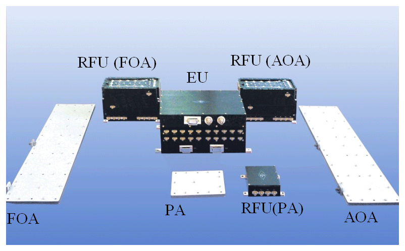
Figure 2The FY3-C GNSS occultation sounder GNOS. The GNOS instrument consists of one electronic unit (EU), two fixed occultation antennas (one forward occultation antenna, FOA, and one aft occultation antenna, AOA), one position antenna (PA), and three radio frequency units (RFUs).
The purpose of this study is to explore applications of FY3-C GNOS ionospheric data products in space weather research, specifically in the analysis of ionospheric NmF2 patterns during the magnetic storm of March 2015, which significantly affected the ionosphere (e.g., Astafyeva et al., 2015; Nava et al., 2016). Results of the study lay the foundation for the use of GNOS in space weather research, including magnetic and ionospheric storms.
The instrument GNOS aboard the FY3-C satellite (in Fig. 2) is composed of one electronic unit (EU), two fixed occultation antennas (one forward occultation antenna, FOA, and one aft occultation antenna, AOA), one position antenna (PA), and three radio frequency units (RFUs). The electronic unit is located in the cabin. The forward and aft occultation antennae are each electrically split into atmospheric and ionospheric components (Bai et al., 2014). The ionospheric occultation antennas are single-unit, micro-strip, dual-mode, and dual-frequency, and they can simultaneously receive BDS dual-frequency (B1I 1561.098 MHz and B2I 1207.140 MHz) and GPS dual-frequency (L1 1575.420 MHz and L2 1227.600 MHz) ionospheric occultation signals. The maximum gain of each antenna is 5 dB, and the half power beam width of the ionospheric occultation antenna is ±40∘. The forward ionospheric occultation antenna is oriented normal to the +x axis of the satellite, i.e., the direction in which the satellite is moving. The aft ionospheric occultation antenna is oriented normal to the −x axis of the satellite. The objective of this design is to make the beam of the ionospheric occultation antenna with maximum gain cover the ionospheric occultation target region, in order to obtain a high signal-to-noise-ratio (SNR) and a high-quality occultation signal.
Within the power consumption limits aboard the FY3-C satellite, GNOS is equipped with six dual-frequency GPS occultation channels, which are able to simultaneously track dual-frequency signals from six GPS satellites (including atmospheric and ionospheric occultation signals). It also has four dual-frequency BDS occultation channels, which can simultaneously track four dual-frequency BDS satellite signals (including atmospheric and ionospheric occultation signals). The GNOS ionospheric occultation data mainly include dual-system, dual-frequency carrier phase and SNR information, with a sampling rate of 1 Hz. Since the primary mission is atmospheric occultation sounding, this is given priority, so that when there are no free channels, a new atmospheric occultation event occupies an ionospheric occultation channel. Under these limited channel conditions, the actual number of complete ionospheric occultation profiles that can be produced daily is around 220 from the GPS and around 130 from the BDS. Since the FY3-C satellite is in a sun-synchronous polar orbit, it passes ground stations at around 10:00 and 22:00 (LT); hence, occultation events are mainly concentrated in the two local time periods between 09:00 and 12:00 and 21:00 and 24:00.
GNSS signals transmitted through the ionosphere and received by LEO satellites are bent and delayed by refraction in the ionosphere. Using dual-frequency phase observations, the corresponding total electron content (TEC) of the ionosphere can be obtained:
where L1 and L2 are the dual-frequency carrier phase observations, C=40.3082 m3 s−2 is a constant, and f1 and f2 indicate the two frequencies. This type of dual-frequency TEC inversion method (Schreiner et al., 1999; Jin et al., 2014) eliminates clock errors (Jin et al., 2014) and uses an Abel transformation to obtain the ionospheric electron density based on the assumption of local spherical symmetry ionosphere:
where Ne(r) is electron density, r0 is the straight-line impact distance, and r is the distance between the earth geometrical center and one point on the ray path.
We evaluated the GNOS ionosphere electron density profiles through statistical comparison with ionosonde data; for detailed comparing results, we refer to Yang et al. (2018). Electron density profile data were collected from GNOS, covering a 365-day period between 1 October 2013 and 30 September 2014, giving 62 381 occultation profiles from the GPS and 47 490 from the BDS. We collected ionosphere observation data taken from ground ionosonde stations, which mainly comprised two parameters: maximum electron density in the F2 layer of the ionosphere (NmF2) and the altitude of the maximum electron density (hmF2). Ionosonde data were obtained from 54 ionosonde stations of the Global Ionospheric Radio Observatory (GIRO) of the University of Massachusetts Lowell (UML) (as shown in Fig. 3). The criteria used for matching GNOS and ionosonde data were a time interval within ±1 h and spherical distance within 200 km. For every matching pair of data, the relative error (R) in the GNOS NmF2 was calculated using Eq. (3):
where the subscript IONO represents ionosonde.
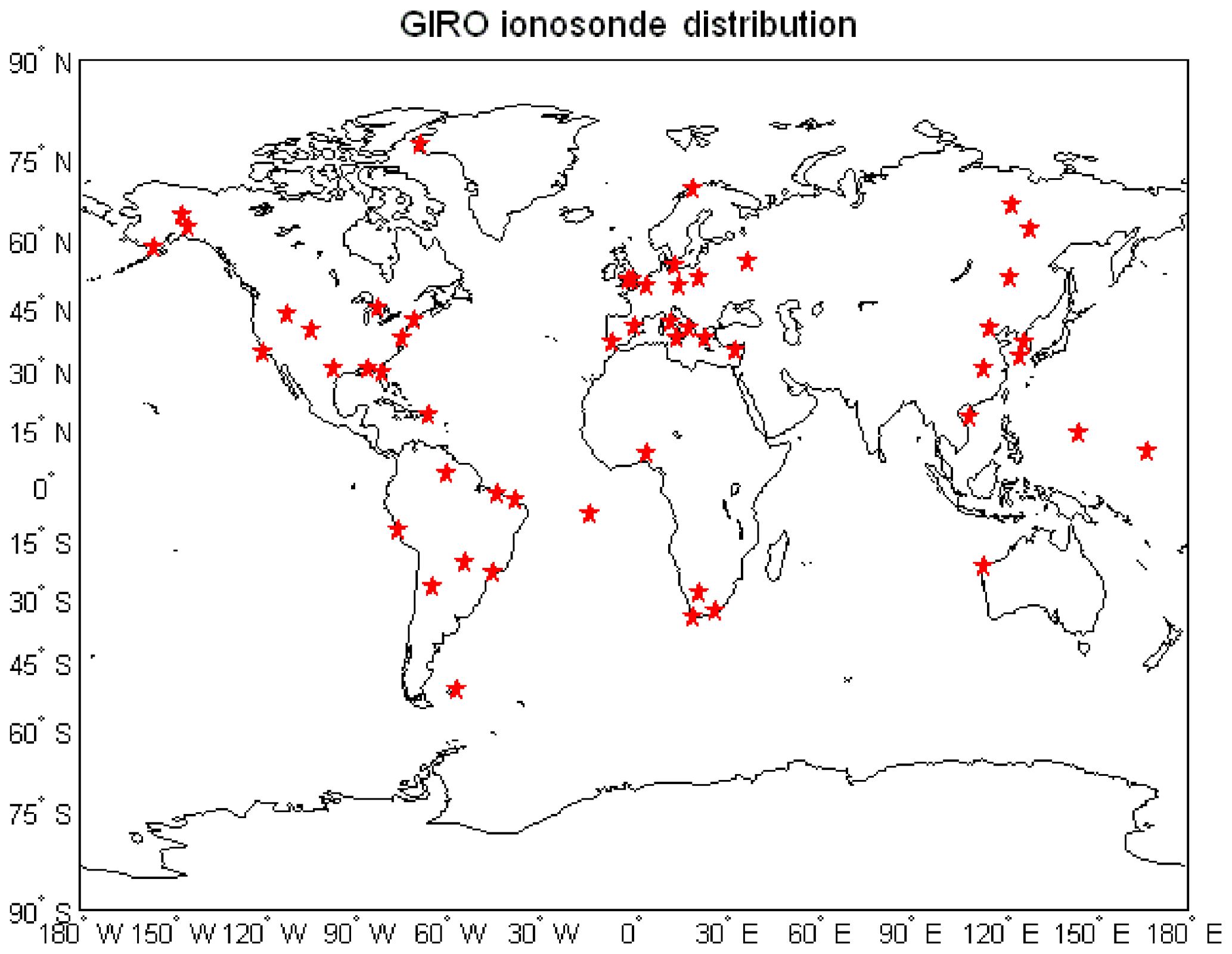
Figure 3The distribution of ionosonde stations. The data of 54 ionosonde stations can be obtained from GIRO.
Figure 4 compares NmF2 and hmF2 measurements from the GNOS GPS occultation and the ionosondes. Over the course of the year, a total of 745 matching pairs of data were collected. Linear regression of absolute NmF2 values derived from each method (Fig. 4) gives a correlation coefficient of 0.96, a statistical bias of 6.71 %, and standard deviation of 18.03 %. The hmF2 correlation coefficient is 0.85, the bias is 4.68 km, and standard deviation is 25.96 km. Figure 5 is similar to Fig. 4 but with GNOS BDS occultation profiles (354 BDS matching pairs) rather than GPS products; the NmF2 correlation coefficient of the fitted regression is 0.96, the statistical bias is 8.31 %, and standard deviation is 17.24 %. The linear regression of hmF2 values derived from the GNOS BDS occultation and ionosonde data gives a correlation coefficient of the fitted regression of 0.80, a statistical bias of 2.67 km, and standard deviation of 23.28 km. The bias and standard deviation of the NmF2 derived from the GNOS BDS occultation and GPS occultation are consistent and comparable. However, the bias and standard deviation of the NmF2 from BDS are slightly larger; this could be caused by the larger position errors of the BDS satellites, especially for the GEO satellites, and the different distribution of the occultation events.
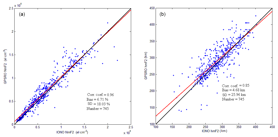
Figure 4Comparison of NmF2 measurements from GNOS GPS occultation and ionosondes. Panel (a) shows a linear regression of the absolute NmF2 values measured using the two methods. The black line is y=x, the red line is the fitted regression, corr. coef. is the correlation coefficient, bias is the statistical bias, and SD is the standard deviation. Panel (b) shows a linear regression of the absolute hmF2 values measured using the two methods (source: Yang et al., 2018).
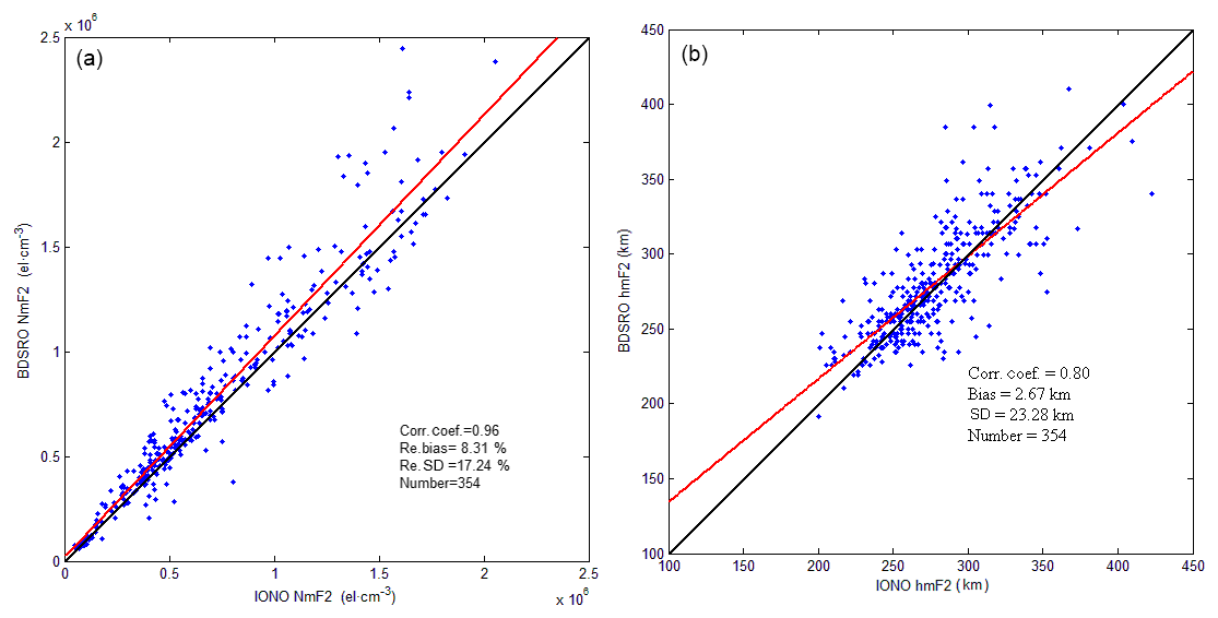
Figure 5Same as Fig. 4, but for GNOS Beidou navigation system (BDS). Comparison of NmF2 and hmF2 measurements from GNOS BDS occultation and ionosondes. Panel (a) shows a NmF2 linear regression fit between the two sets of measurements; panel (b) shows a hmF2 linear regression fit between the two sets of measurements.
Global electron density profiles have been successfully probed in several previous GNSS radio occultation missions, including GPS/MET, CHAMP, and COSMIC (e.g., Garcia-Fernandez et al., 2003; Habarulema et al., 2014). Using ionosonde data for verification, their reported precisions are NmF2 average bias 1 % and standard deviation 20 % for GPS/MET (Hajj et al., 1998) and NmF2 average bias −1.7 % and standard deviation 17.8 % for CHAMP (Jakowski et al., 2002). The mean differences of the Nmf2 are insignificant for COSMIC; relative variations of the peak differences are determined in the range of 22 %–30 % for NmF2 and 10 %–15 % for hmF2 (Limberger et al., 2015). In particular, even during disturbed conditions, the relative difference of NmF2 and hmF2 agrees to within 21 % and 9 %, respectively, as reported by Habarulema et al. (2016), who made the first long-term comparison between RO and ionosonde NmF2 and hmF2 data over Grahamstown. GNOS GPS and BDS occultation NmF2 observations reported in this study have a slightly higher average bias than the other systems, but their good correlation coefficients and standard deviations demonstrate the overall reliability of the results.
3.1 Characteristics of the magnetic storm
Solar activity in 2015 was at a moderate level, and there were several large geomagnetic storm events. This study focuses on the magnetic storm event that occurred between 11 and 31 March 2015, peaking at 05:22 UT on 17 March. Changes in magnetic indices during the storm are shown in Fig. 6. The geomagnetic activity index Kp, which characterizes global geomagnetic activity, was generally below 3 before 17 March, then it increased significantly, with large perturbations continuing until 26 March, after which it returned to pre-storm levels. The Dst index, which is an index of geomagnetic activity used to assess the severity of magnetic storms, was relatively stable before 17 March, hovering around zero. The index suddenly increased between 04:00 and 06:00 UT on 17 March, marking the initial phase of the magnetic storm, and then dropped rapidly during the main phase to a minimum of −223 nT at 23:00 UT. A rapid recovery phase followed, from 23:00 UT on 17 March until 18:00 UT on 18 March, then a slower recovery until around 10:00 UT on 25 March, when it returned to pre-storm levels. The auroral electrojet (AE) index mainly reflects polar substorm intensity, with variations closely related to the quantity of particles injected into polar regions. The AL and AU indices reflect westward and eastward electrojet conditions, and the AE index is the absolute difference between them. During the main phase of the magnetic storm, the magnitude of AE index perturbations reached around 1500, with frequent lower magnitude perturbations during the recovery phase. Overall, this magnetic storm event caused severe geomagnetic disturbances on a global scale. As plasma in the ionosphere is controlled by the earth's magnetic field, the global ionosphere was also affected by the magnetic storm.
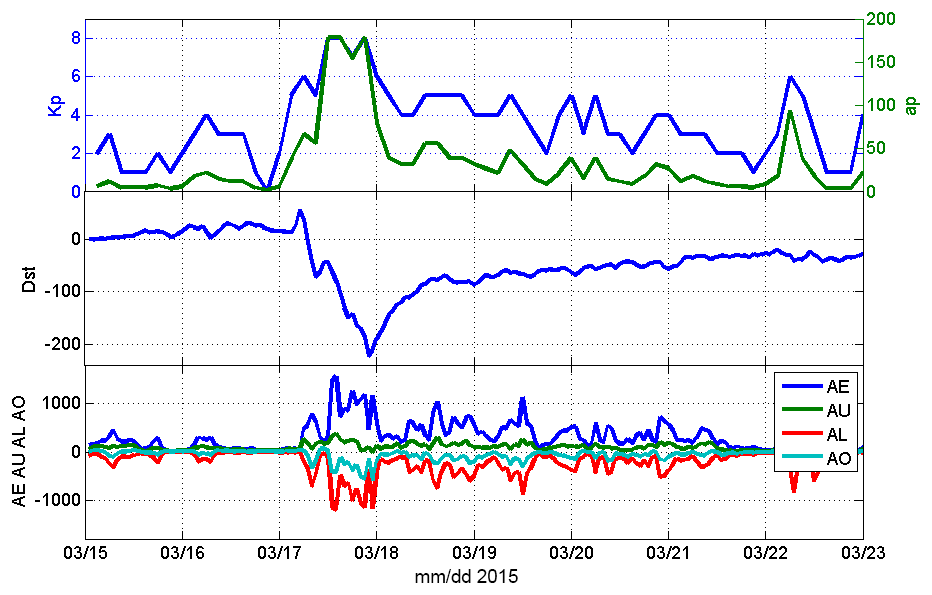
Figure 6Variations of geomagnetic indices (Kp, ap, Dst, AE, AU, AL, and AO) during the magnetic storm of March 2015 (data from the International Service of Geomagnetic Indices (ISGI) website: http://isgi.latmos.ipsl.fr/ (last access: 10 September 2016)).
3.2 Global GNOS results during the magnetic storm
Figure 7 shows global daytime (07:00–17:00 LT; Fig. 7a) and nighttime (19:00–05:00 LT; Fig. 7b) occultation event distributions for 14 March 2015 (pre-storm calm), 17 March (main phase), 18 March (rapid recovery phase), and 22 March (recovery phase). Around 350 ionosphere occultation profiles were recorded daily (220 GPS + 130 BDS). Although the quantity of data is limited due to the rather high inclination polar orbit of FY3-C, recorded occultation events are distributed across the globe, with a relative concentration at higher latitudes. Figure 7a shows that, before the magnetic storm, the highest daytime NmF2 values were mostly distributed around the magnetic equator, with relatively low electron densities at high magnetic latitudes. During the main phase of the storm, NmF2 perturbations were significant, with especially large increases in the South Atlantic region. In the southeastern Pacific, NmF2 decreased during the main storm phase and increased during the recovery phase, returning to pre-storm levels by 22 March. Nighttime GNOS soundings (Fig. 7b) show suppressed NmF2 values in East Asia and Australia during the main phase and start of the recovery phase of the storm. NmF2 values had returned to pre-storm levels by 22 March. These results demonstrate the capability of FY3-C GNOS to characterize the global NmF2 response to magnetic storm events.
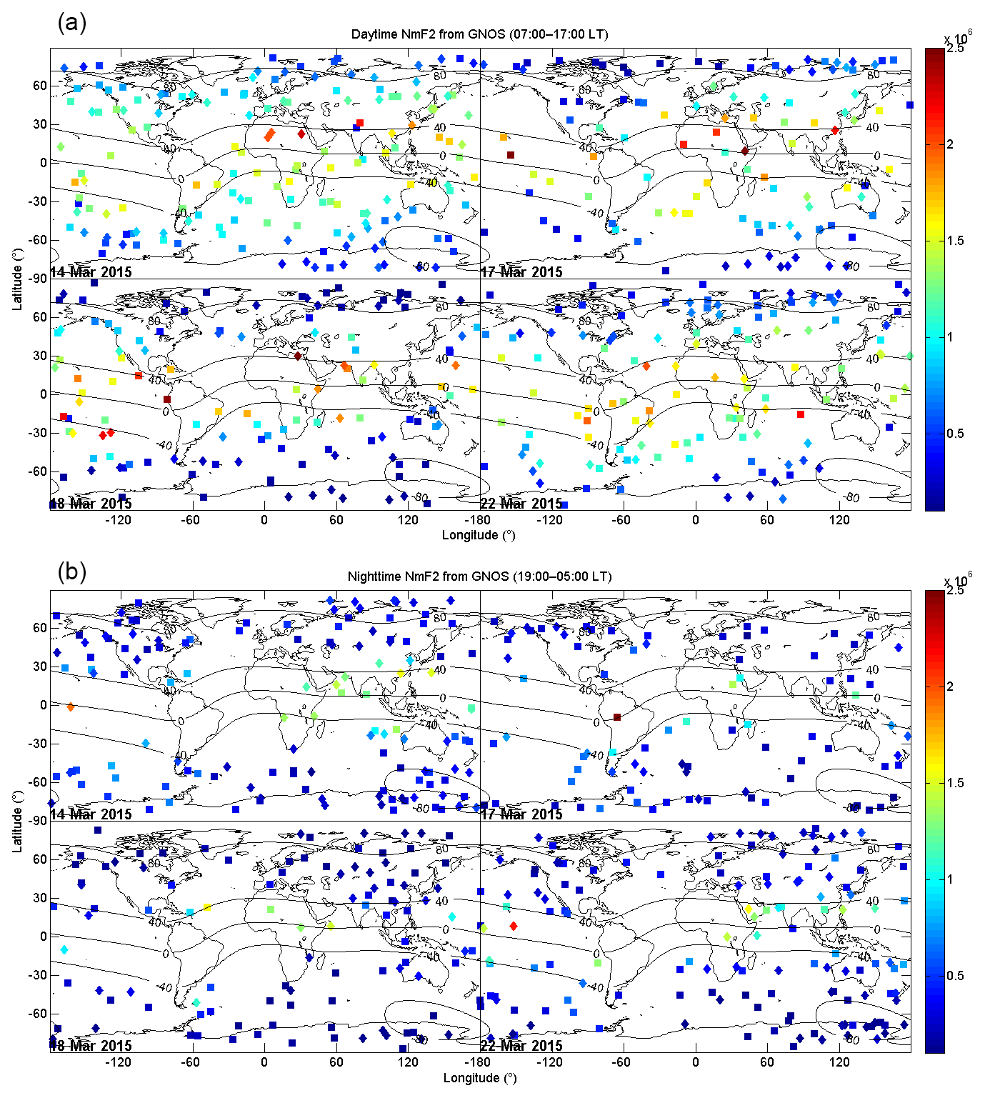
Figure 7(a) NmF2 values detected by GNOS in all daytime (07:00–17:00 LT) occultation events on typical representative days (14 March calm, 17 March magnetic storm main phase, 18 March rapid recovery phase, and 22 March steady recovery phase). Squares represent the geographic location of GNOS GPS occultation events. Diamonds represent the geographic location of GNOS BDS occultation events. The color of each square or diamond represents NmF2 magnitude for that occultation event. Black contours represent geomagnetic inclination isolines. (b) Same as (a), but for the NmF2 values detected by GNOS in all nighttime (19:00–5:00 LT) occultation events.
3.3 Statistical analysis of GNOS ionosphere products and ionosonde observations during the magnetic storm period
The daily GNOS ionosphere profiles are relatively sparse and unevenly distributed around the globe. Therefore, it is difficult to quantitatively analyze the response of a specific location during a magnetic storm event. However, as most occultation events are distributed at midlatitudes and high latitudes (magnetic inclinations of 40–80∘ in both hemispheres), it is possible to analyze changes in average NmF2 values in specific zones during a magnetic storm.
We also compare GNOS measurements' statistical analysis with ionosonde data from the US Space Weather Prediction Center (SWPC) worldwide stations and China Meridian Project stations. As there are very few ionosonde stations located at magnetic inclinations of 40–80∘ in the Southern Hemisphere, we focused on NmF2 data from the 15 ground stations in the Northern Hemisphere in the period 14–22 March 2015. The geographic distribution of these 15 stations, including 13 SWPC ionosonde stations and two China Meridian Project stations, is shown in Fig. 8. According to the distribution of these stations, we classify these stations into two zones. Zone 1, including eight SWPC stations, is within magnetic inclinations of 40–80∘ and longitudes of −20–40∘, mainly in the Europe region. Zone 2, including five SWPC stations and two China Meridian Project stations, is located within magnetic inclinations of 40–80∘ and longitudes of 100–160∘, mainly in the East Asia region.
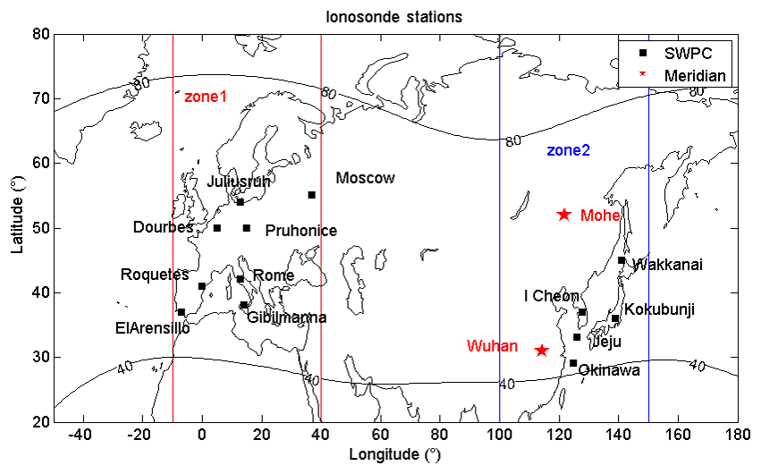
Figure 8Distribution of ionosonde stations located in two zones. Zone 1, including eight SWPC stations, is within magnetic inclinations of 40–80∘ and longitudes of −20–40∘, mainly in the Europe region. Zone 2, including five SWPC stations and two China Meridian Project stations, is located within magnetic inclinations of 40–80∘ and longitudes of 100–160∘, mainly in the East Asia region. Black squares represent SWPC stations, and red stars represent China Meridian Project stations.
Figures 9 and 10 plot NmF2 variations at each station in zone 1 and zone 2, respectively; blue lines denote the SWPC stations, and the red lines denote the China Meridian Project stations. Perhaps the most outstanding feature is a surge in NmF2 values at individual stations on 17 March, during the main phase of the magnetic storm (e.g., around 12:00 LT at Moscow), with a decrease after 16:00 at many stations. Several stations show a significant decrease in NmF2 measurements during the beginning of the recovery phase, on 18 and 19 March, except for a few European stations in zone 1 (e.g., Rome). After 19 March, NmF2 patterns become more complex, with some stations (e.g., Mohe) showing values below pre-storm levels and others (e.g., Okinawa) about the same as pre-storm levels. Overall, ionospheric perturbations during the magnetic storm were mainly negative.
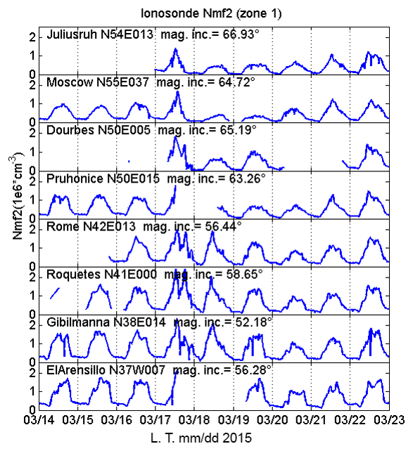
Figure 9Variations in NmF2 at eight ground ionosonde stations located in zone 1 during the magnetic storm of March 2015. Ionosonde data were obtained from SWPC.
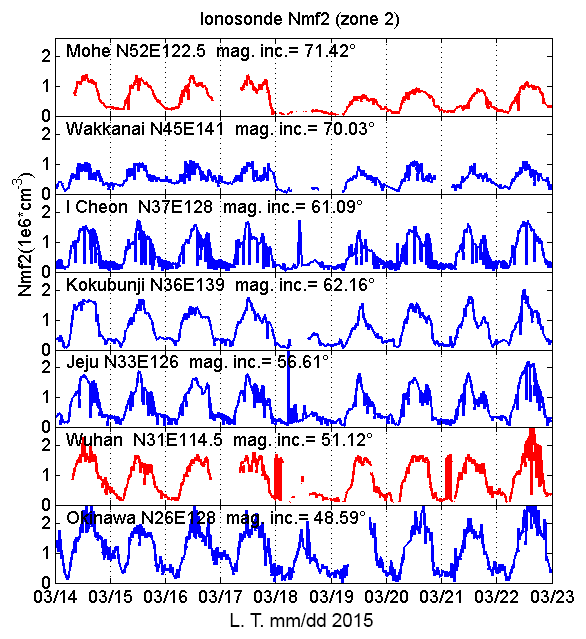
Figure 10Variations in NmF2 at five SWPC stations and two China Meridian Project ground ionosonde stations in zone 2 during the magnetic storm of March 2015. The blue lines represent the SWPC station, and the red lines denote the China Meridian Project station.
Figure 11a and b compare error bars of NmF2 values from the ionosonde stations with those from the GNOS occultation products in two zones, respectively, for different time periods in the magnetic storm event, including 9:00–12:00 and 21:00–24:00 LT (most of the GNOS occultation events were concentrated around these times). Figure 11a compares error bars in zone 1, mainly in the Europe region, and Fig. 11b represents the results in zone 2, mainly in the East Asia region. In these plots, NmF2 trends are very similar for the two observation methods, with the negative storm effects of the recovery phase quite clear. However, GNOS measurements, especially in the 21:00–24:00 LT time block, show larger perturbations than those of the ionosonde stations. These discrepancies may be due to the significant differences of the spatial observations between the two measurement techniques; i.e., GNOS can observe randomly, whereas the locations of the ionosondes are fixed on the continents. Nighttime (21:00–24:00 LT) average NmF2 levels were much lower in the main phase (17 March) and at the start of the recovery phase (18–20 March) than before the storm, reaching a minimum on 18 March. Then, the average NmF2 levels rose slowly during the whole recovery phase. Daytime average NmF2 in zone 2 reached a maximum during the main phase of the magnetic storm on 17 March, falling to a minimum on 19 March, after which it slowly increased. In zone 1 in Fig. 11a, daytime average NmF2 is shown to have reached a minimum on 18 March from GNOS data, but it reached a minimum on 20 March and then slowly recovered.

Figure 11(a) Comparison of error bars of NmF2 values from the eight ionosonde stations and GNOS in zone 1 in the Northern Hemisphere during the magnetic storm of March 2015. (b) Same as (a), but for the comparison of error bars of NmF2 values from the seven ionosonde stations and GNOS in zone 2.
Overall, the magnetic storm caused significant disturbances in average NmF2 in both zone 1 and zone 2. Both daytime and nighttime NmF2 values showed mainly negative storm characteristics; NmF2 decreased significantly during the main phase of the storm and increased tardily during the recovery phase.
The GNSS radio occultation allows monitoring of electron density in the ionosphere at a global scale. It has the advantages of high accuracy, good vertical resolution, global coverage, and all-weather capability. However, an important constraint in applications of the occultation electron density products is the assumption of a symmetrical ionosphere in the inverse Abel transformation calculations (Garcia-Fernandez et al., 2003; Yue et al., 2010, 2011). In reality, it is very difficult to guarantee symmetrical distribution of electron density in the ionosphere, especially near anomalies at the magnetic equator and high latitudes. Nevertheless, comparison of the GNOS probe results with ionosonde measurements provided a correlation coefficient of 0.95 and standard deviation less than 20 %, which are basically coincident with previous studies (e.g., Habarulema et al., 2016). Therefore, in the majority of cases, GNOS results may be considered to be reliable and reasonable.
The March 2015 magnetic storm was up to now the strongest in the recent solar cycle and severely disturbed the global ionosphere, which has been extensively investigated. For instance, Astafyeva et al. (2015) have shown multi-instrumental results on the global ionospheric response to the storm. Nava et al. (2016) have also presented the effects of the storm over the midlatitude and low-latitude ionosphere in Asian, African, American, and Pacific sectors using global and regional electron content. Here, we analyzed the effect of the March 2015 magnetic storm on the global ionosphere using data from FY3-C GNOS and from ground-based ionosonde stations. In terms of spatial distribution, Fig. 7a shows that the daytime NmF2 values in the South Atlantic region were elevated during the main phase of the storm compared with ones on 14 March before the storm. This increase in NmF2 during the main phase also occurred in the northern Africa region, which is consistent with the ionospheric positive storm effect reported in Fig. 3 of Astafyeva et al. (2015) and in Fig. 4 of Nava et al. (2016). In the southeastern Pacific, the daytime NmF2 values seemed to decrease a little during the main phase of the storm, and then they increased in the recovery phase. This is little different from the results of Astafyeva et al. (2015), who presented a significant positive storm effect during the main phase and a negative storm at the beginning of the recovery phase at low latitudes in the eastern Pacific sector. This difference may be due to the fact that their focused latitude region is lower than ours. Figure 7b shows that the nighttime NmF2 values around the East Asia and Australia sector were mainly suppressed during the main phase and at the beginning of the recovery phase then returned to pre-storm levels by 22 March. These results are consistent with those reported by Nava et al. (2016).
It was not possible to perform long-term continuous comparison between ionosonde and GNOS data, as the number of occultation events recorded by GNOS was insufficient. Hence, the results from two zones were averaged to enable a quantitative comparison. In addition, the statistical significance of this method is based on the assumption that the effects of the magnetic storm are basically consistent throughout the ionosphere in each zone. Figure 11a and b display the statistical comparison of the averaged data, showing similar general trends in measurements from the ionosonde stations and GNOS during the storm. The comparison further confirmed the nature of the magnetic storm and the negative effects of the storm on the ionosphere. The negative storm in ionosphere parameters is usually caused by composition changes. During the storm, the high-latitude atmosphere will be heated heavily, which results in upwelling of the molecular rich neutral gas into the upper thermosphere and provokes the neutral gas circulation from the pole to the Equator (e.g., Fuller-Rowell et al., 1996). Furthermore, the ion density loss is proportional to the molecular concentration; thus the negative storm will occur over the regions where the molecular mass increases. In Fig. 9, a few stations (such as Gibilmanna) are shown to have observed a sustained daytime NmF2 enhancement on 18 March. The exact reasons for this enhancement are not clear. The major contributors could include neutral composition changes (Crowley et al., 2006), thermospheric winds (Balan et al., 2011), disturbance of the dynamo electric field (Richmond and Lu, 2000), or some combination of these factors. In fact, the way in which the global ionosphere responds to magnetic storms is extremely complicated. From Fig. 7a, we can see that this particular magnetic storm caused varying responses in the ionosphere at different times and locations. Many factors influence the ionosphere, such as neutral composition changes, electric fields, and neutral winds. For a specific magnetic storm, corresponding ionospheric perturbations also depend on the season, solar activity, local time of magnetic storm occurrence, and the latitude and longitude. Therefore, ionospheric storms are extremely complex; no two storms are precisely alike, and the mechanisms that generate them also vary (Balan et al., 1990; Fuller-Rowell et al., 1996; Danilov et al., 2001; Mendilo et al., 2006). In addition, the type and form of a magnetic storm also make a difference in the way that it affects the ionosphere (Zhang et al., 1995). Future analysis incorporating assimilation with other data sources and models may allow the precise mechanisms responsible for ionospheric effects of the March 2015 magnetic storm to be determined.
The comparison of ionosonde data and FY3-C GNOS radio occultation products presented in this study shows that, in the majority of cases, GNOS NmF2 data are reliable and reasonable. Based on ionosphere data from the FY3-C GNOS payload combined with those from ground-based ionosonde, this study analyzed the characteristics of the global ionosphere response to the magnetic storm event in March 2015. Daytime NmF2 values increased in the South Atlantic region, and they first decreased and then increased in the southeast Pacific region. In East Asia and Australia, nighttime NmF2 values were mainly suppressed but recovered to pre-storm levels around 22 March. In the region of higher magnetic inclinations, NmF2 levels were clearly affected by the storm. Daytime and nighttime NmF2 levels mainly indicated a negative storm response. Overall, the trends detected by GNOS during the magnetic storm event in two zones of magnetic inclinations between 40 and 80∘ in the Northern Hemisphere were similar to the trends detected by the ground-based ionosonde stations. This further confirmed the negative response of the ionosphere to the March 2015 magnetic storm event. The study demonstrates the reliability of FY3-C GNOS radio occultation measurements for analyzing statistical and event-specific physical characteristics of the ionosphere. More Beidou navigation satellites and other FY3 series satellites (FY3-D, E, F, G, and R) are planned in the future, and their GNOS payloads offer the potential for the generation of significantly more data in support of ionospheric physics research and forecasting applications.
The data of China Meridian Project are available at https://data.meridianproject.ac.cn/ (last access: 10 August 2016). The data of FY3-C GNOS are available at http://satellite.nsmc.org.cn/portalsite/Data/DataView.aspx (last access: 10 August 2016). The data of SWPC are available at ftp://ftp.swpc.noaa.gov/pub/lists/iono_month/ (last access: 10 August 2016).
The authors declare that they have no conflict of interest.
We thank UML GIRO and SWPC for providing the ionosonde data. We also
acknowledge the use of data from the Chinese Meridian Project. This research
was supported jointly by the National Science Fund of China (41505030, 41405039,
41405040, 41574150, 41606206, 41674145, and 41474137) and the Scientific Research
Project of the Chinese Academy of Sciences (YZ201129), as well as the
Specialized Research Fund for State Key Laboratories of China.
Edited by: Andreas Richter
Reviewed by: Chris Watson and one anonymous referee
Astafyeva, E., Zakharenkova, I., and Förster, M.: Ionospheric response to the 2015 St. Patrick's Day storm: A global multi-instrumental overview, J. Geophys. Res.-Space, 120, 9023–9037, 2015.
Bai, W. H., Sun, Y. Q., Du, Q. F., Yang, G. L., Yang, Z. D., Zhang, P., Bi, Y. M., Wang, X. Y., Cheng, C., and Han, Y.: An introduction to the FY3 GNOS instrument and mountain-top tests, Atmos. Meas. Tech., 7, 1817–1823, https://doi.org/10.5194/amt-7-1817-2014, 2014.
Balan, N. and Rao, P. B.: Dependence of ionospheric response on the local time of sudden commencement and the intensity of geomagnetic storms, J. Atmos. Terr. Phys., 52, 269–275, 1990.
Balan, N., Yamamoto, M., and Liu, J. Y.: New aspects of thermospheric and ionospheric storms revealed by CHAMP, J. Geophys. Res., 116, A07305, https://doi.org/10.1029/2010JA016399, 2011.
BeiDou navigation satellite system signal in space interface control document open service signal (Version 2.1): http://en.beidou.gov.cn/, last access: November 2016.
Crowley, G., Hackert, C. L., Meier, R. R., Strickland, D. J., Paxton, L. J., Pi, X., Mannucci, A., Christensen, A. B., Morriston, D., Bust, G. S., Roble, R. G., Curtis, N., and Wene, G.: Global thermosphere-ionosphere response to onset of 20 November 2003 storm, J. of Geophys. Res., 111, A10S18, https://doi.org/10.1029/2005JA011518, 2006.
Danilov, A. D.: F2-region response to geomagnetic disturbances, J. Atmos. Sol.-Terr. Phy., 63, 441–449, 2001.
Fu, E. J., Zhang, K. F., Wu, F. L., Xu, X. H., and Marion, K. : An Evaluation of GNSS Radio Occultation Technology for Australian Meteorology, Positioning, 6, 74–79, 2007.
Fuller-Rowell, T. J., Codrescu, M. V., Rishbeth, H., Moffett, R. J., and Quegan, S.: On the seasonal response of thermosphere and ionosphere to magnetic storms, J. Geophys. Res., 101, 2343–2353, https://doi.org/10.1029/95JA01614, 1996.
Garcia-Fernandez, M., Hernandez-Pajares, M., Juan, M., and Sanz, J.: Improvement of ionospheric electron density estimation with GPSMET occultations using Abel inversion and VTEC information, J. Geophys. Res., 108, 1338–1345, https://doi.org/10.1029/2003JA009952, 2003.
Habarulema, J. B., Katamzi, Z. T., and Yizengaw, E.: A simultaneous study of ionospheric parameters derived from FORMOSAT-3/COSMIC, GRACE, and CHAMP missions over middle, low, and equatorial latitudes: Comparison with ionosonde data, J. Geophys.l Res.-Space, 119, 7732–7744, 2014.
Habarulema, J. B. and Carelse, S. A.: Long-term analysis between radio occultation and ionosonde peak electron density and height during geomagnetic storms, Geophys. Res. Lett., 43, 4106–4111, 2016.
Hajj, G. A. and Remans, L.: Ionospheric electron density profiles obtained with the global positioning system: Results from the GPS/MET experiment, Radio Sci., 33, 175–190, 1998.
Hocke, K., Igarashi, K., Nakamura, M., Wilkinson, P., Wu, J., Pavelyev, A., and Wickert, J.: GIobal sounding of sporadic E layers by the GPS/MET radio occultation experiment, J. Atmos. Sol.-Terr. Phy., 63, 1973–1980, 2001.
Jakowski, N., Wehrenpfennig, A., Heise, S., Reigber, Ch., and Lühr, H.: GPS radio occultation measurements of the ionosphere from CHAMP: Early results, Geophys. Res. Lett., 29, 2–4, 2002.
Jin, S., Estel, C., and Xie, F. (Eds.): GNSS remote sensing theory, methods and applications, EARSel Series, Springer, Freek D., Netherlands, 2014.
Liao, M., Zhang, P., Yang, G.-L., Bi, Y.-M., Liu, Y., Bai, W.-H., Meng, X.-G., Du, Q.-F., and Sun, Y.-Q.: Preliminary validation of the refractivity from the new radio occultation sounder GNOS/FY-3C, Atmos. Meas. Tech., 9, 781–792, https://doi.org/10.5194/amt-9-781-2016, 2016.
Limberger, M., Hernández-Pajares, M., Aragón-Ángel, A., Altadill, D., and Dettmering, D.: Long-term comparison of the ionospheric F2 layer electron density peak derived from ionosonde data and Formosat-3/COSMIC occultations, J. Space Weather Spac., 5, A21, https://doi.org/10.1051/swsc/2015023, 2015.
Liu, L. B., He, M. S., Wan, W. X., and Zhang, M. L.: Topside ionospheric scale heights retrieved from Constellation Observing System for Meteorology, Ionosphere, and Climate radio occultation measurements, J. Geophys. Res.-Space, 113, 1429–1443, https://doi.org/10.1029/2008JA013490, 2008.
Liu, L. B., Zhao, B. Q., Wan, W. X., Ning, B. Q., Zhang, M. L., and He, M. S.: Seasonal variations of the ionospheric electron densities retrieved from Constellation Observing System for Meteorology, Ionosphere, and Climate mission radio occultation measurements, J. Geophys. Res.-Space, 114, 1–11, https://doi.org/10.1029/2008JA013819, 2009.
Liu, L. B., He, M. S, Yue, X. A., Ning, B. Q., and Wan, W. X.: Ionosphere around equinoxes during low solar activity, J. Geophys. Res.-Space, 115, 1–10, https://doi.org/10.1029/2010JA015318, 2010.
Liu, L. B., Le, H. J., Chen, Y. D., He, M. S, Wan, W. X., and Yue, X. A.: Features of the middle- and low-latitude ionosphere during solar minimum as revealed from COSMIC radio occultation measurements, J. Geophys. Res.-Space, 116, 1161–1166, https://doi.org/10.1029/2011JA016691, 2011.
Lu, H. and Zou, Y.: Research on the global morphological features of spread F based on GPS occultation observation, Journal of Guilin University of Electronic Technology, 31, 508–512, 2011.
Mendilo, M.: Storms in the ionosphere: patterns and processes for total electron content, Rev. Geophys., 44, 335–360, 2006.
Nava, B., Rodríguez-Zuluaga, J., Alazo-Cuartas, K., Kashcheyev, A., Migoya-Orué, Y., Radicella, S. M., Amory-Mazaudier, C., and Fleury, R.:, Middle- and low-latitude ionosphere response to 2015 St. Patrick's Day geomagnetic storm, J. Geophys. Res.-Space, 121, 3421–3438, https://doi.org/10.1002/2015JA022299, 2016.
Richmond, A. and Lu, G.: Upper-atmospheric effects of magnetic storms: A brief tutorial, J. Atmos. Sol.-Terr. Phys., 62, 1115–1127, 2000.
Schreiner, W, Sokolovskiy, S, Rocken, C, and Hunt, D.: Analysis and validation of GPS/MET radio occultation data in the ionosphere, Radio Sci., 34, 949–966, 1999.
Wang, S. Z., Zhu, G. W., Bai, W. H., Liu, C. L., Sun, Y. Q., Du, Q. F., Wang, X. Y., Meng, X. G., Yang, G. L., Yang, Z. D., Zhang, X. X., Bi, Y. M., Wang, D. W., Xia, J. M., Wu, D., Cai, Y. R., and Han, Y.: For the first time fengyun3 C satellite-global navigation satellite system occultation sounder achieved spaceborne Bei Dou system radio occultation, Acta Phys. Sin.-Ch. Ed., 64, 9301, https://doi.org/10.7498/aps.64.089301, 2015.
Yang, G. L.: Ionospheric Radio Occultation by GNOS, Ph.D. thesis, University of Chinese Academy of Science, China, 2015.
Yang, G. L., Sun, Y. Q., Bai, W. H., Zhang, X. X., Liu, C. L., Meng, X. G., Bi, Y. M., Wang, D. W., and Zhao, D. Y.: Validation results of NmF2 and hmF2 derived from ionospheric density profiles of GNOS on FY-3C satellite, Sci China Tech Sci, 61, 1–12, https://doi.org/10.1007/s11431-017-9157-6, 2018.
Yang, J., Wu, Y., and Zhou, Y.: Research on Seismo-Ionospheric Anomalies Using GPS Radio Occultation Data, J. Geodesy Geodynam., 28, 16–22, 2008.
Yue, X., Schreiner, W. S., Lei, J., Sokolovskiy, S. V., Rocken, C., Hunt, D. C., and Kuo, Y.-H.: Error analysis of Abel retrieved electron density profiles from radio occultation measurements, Ann. Geophys., 28, 217–222, https://doi.org/10.5194/angeo-28-217-2010, 2010.
Yue, X., Schreiner, W., S., et al.: Evaluation of the orbit altitude electron density estimation and its effect on the Abel inversion from radio occultation measurements, Radio Sci., 46, 247–249, 2011.
Zhang, Q. W., Guo, J. S., Zhang, G. L., and Zheng, H.: Mid-and low-latitude ionospheric responses to different type of magnetic storm, Chinese J. Geophys.-Ch., 38, 581–589, 1995.
Zhang, X., Hu, X., and Zhang, C.: Ionospheric Response with Wenchuan Big Earthquake by Occulted Data, GNSS World of China, 5, 1–5, 2008.
Zhao, B. Q., Wang, M., Wang, Y. G., Ren, Z. P., Yue, X. A., Zhu, J., Wan, W. X., Ning, B. Q., Liu, J., and Xiong, B.: East-West Differences in F-region Electron Density at Midlatitude: Evidence from the Far East Region, J. Geophys. Res., 118, 542–553, https://doi.org/10.1029/2012JA018235, 2013.