the Creative Commons Attribution 4.0 License.
the Creative Commons Attribution 4.0 License.
 | 13 Mar 2019
Improvement of airborne retrievals of cloud droplet number concentration of trade wind cumulus using a synergetic approach
André Ehrlich
Marek Jacob
Susanne Crewell
Martin Wirth
Manfred Wendisch
In situ measurements of cloud droplet number concentration N are limited by the sampled cloud volume. Satellite retrievals of N suffer from inherent uncertainties, spatial averaging, and retrieval problems arising from the commonly assumed strictly adiabatic vertical profiles of cloud properties. To improve retrievals of N it is suggested in this paper to use a synergetic combination of passive and active airborne remote sensing measurement, to reduce the uncertainty of N retrievals, and to bridge the gap between in situ cloud sampling and global averaging. For this purpose, spectral solar radiation measurements above shallow trade wind cumulus were combined with passive microwave and active radar and lidar observations carried out during the second Next Generation Remote Sensing for Validation Studies (NARVAL-II) campaign with the High Altitude and Long Range Research Aircraft (HALO) in August 2016. The common technique to retrieve N is refined by including combined measurements and retrievals of cloud optical thickness τ, liquid water path (LWP), cloud droplet effective radius reff, and cloud base and top altitude. Three approaches are tested and applied to synthetic measurements and two cloud scenarios observed during NARVAL-II. Using the new combined retrieval technique, errors in N due to the adiabatic assumption have been reduced significantly.
- Article
(4031 KB) - Full-text XML
- BibTeX
- EndNote


Clouds influence the Earth's radiative energy budget by reflecting, absorbing, and emitting solar and terrestrial radiation. These effects are typically quantified by the cloud radiative forcing (CRF), which is defined by the difference between the net radiation (downward minus upward irradiance) in cloudy and cloud-free conditions. Depending on the cloud type, the cloud optical and microphysical properties, and their spatial and temporal occurrence, the CRF can vary significantly (Rosenfeld, 2006). In the tropics, clouds can either cool or warm the atmosphere and surface below the cloud. While for cirrus a warming effect dominates (Wendisch et al., 2007), boundary layer trade wind cumuli typically cool the subjacent atmosphere and surface by efficiently reflecting solar radiation (Warren et al., 1988). Therefore, a realistic representation of clouds in numerical weather prediction (NWP) and global climate models (GCMs) is essential. Due to their sub-grid scale, internal variability, and boundary layer interactions, trade wind cumulus clouds are not well represented in NWP and GCMs (Kollias and Albrecht, 2010). An important source of uncertainty of these models is caused by an insufficient representation of the first aerosol effect (Bony and Dufresne, 2005), which describes the correlation of the cloud droplet number concentration N and the cloud optical thickness τ or cloud-top reflectivity ℛ, commonly known as the Twomey effect (Twomey, 1977). It is most prominent for optically thin, low-level clouds such as trade wind cumulus (Platnick and Twomey, 1994; Werner et al., 2014), which are a ubiquitous cloud type in the tropics (Warren et al., 1988; Eastman et al., 2011). Despite their small vertical and horizontal extent, trade wind cumuli can have fractional cloudiness of more than 25 % (Albrecht, 1991) and therefore may influence the Earth radiative energy budget significantly (Chertock et al., 1993). In addition, trade wind cumuli play an important role in maintaining the thermodynamic energy budget in the atmospheric boundary layer. They couple the surface and free atmosphere by transporting latent heat and developing deep convection (Lamer et al., 2015). Another important factor determining the CRF is the number concentration of aerosol particles, in particular the amount of particles that can act as cloud condensation nuclei (CCN) (Werner et al., 2013). Depending on the CCN number concentration, precipitation formation can be promoted or inhibited (Lee and Feingold, 2013). The CCN concentration influences the cloud life cycle and lifetime (Albrecht, 1989). The magnitude of both effects depends on the individual cloud regime.
Operational NWP models usually do not have the computational capability to consider size-resolved microphysical schemes, and therefore the usage of simplified parameterizations is inevitable. The most important parameter, which links microphysical and radiative properties of clouds, is the cloud droplet effective radius reff, which represents the radiative effective size of a cloud droplet population (Pontikis and Hicks, 1992). In NWP and GCMs, reff is calculated from N and the liquid water content (LWC). In simple models, assumptions of constant N are applied for different situations, e.g., the classification of polluted and clean air masses. As reff is derived from LWC and N, the cloud droplet number concentration is a key parameter for models to calculate reasonable values of reff and to represent the Twomey effect. Also for NWP with two-moment schemes, which use N in addition to the mass mixing ratio, a validation of N as a prognostic variable emerges.
To measure N and LWC, airborne in situ measurements are applied by utilizing different physical methods and instruments (Baumgardner et al., 2011; Wendisch and Brenguier, 2013). These are based on optical measurement principles such as forward scattering, phase Doppler interferometry, and holographic imaging. Beside the uncertainties of the individual measurement techniques, the total sample volume of the instruments is rather limited in comparison to the typical horizontal and vertical extent of clouds. Due to the limited flight time and range, airborne in situ observations cannot cover the natural variability of N, reff, and LWC completely. To directly quantify the Twomey effect, colocated measurements of cloud microphysical and radiative properties are required, which was realized only on a few occasions (Ackerman et al., 2000; Siebert et al., 2013; Werner et al., 2014).
To improve global statistics of estimates of the Twomey effect, several approaches to derive N from satellite observations have been developed (Grosvenor et al., 2018b; Quaas et al., 2009; Minnis et al., 2011; Mace et al., 2016; Bennartz and Rausch, 2017). These techniques provide useful global data sets with large spatial and temporal coverage. Based on passive remote sensing in the solar and terrestrial wavelength range, N is estimated by combining the results of bi-spectral retrievals of τ and reff with cloud-top temperature TCT by Brenguier et al. (2000), Quaas et al. (2006), and Zeng et al. (2014). They assumed a vertically constant LWC and N throughout the cloud profile, which is at least for LWC not a realistic scenario. Slightly deviating, Bennartz and Rausch (2017) assumed a sub-adiabatic vertical profile in which the LWC increases linearly with height with values corresponding to about 80 % of the respective adiabatic value. More complex vertical profile types of LWC and N are applied by Boers et al. (2006), in which a heterogeneous mixing model assumes that entrainment dilutes the air parcel with a constant mean-volume radius of the droplets rvol (the radius of cloud droplets with a volume corresponding to the average of the volume size distribution of the cloud population), while reff follows an adiabatic profile. The retrieved values of N using the homogeneous or the heterogeneous model differ by several percent. Further studies show that the heterogeneous model represents nature more realistically compared to the homogeneous assumption (Boers et al., 1998; Brenguier et al., 2000). These methods often use the dependence of τ on N to connect cloud microphysical and radiative properties. However, so far no operational satellite products of N are available. Retrievals of N, in general, can have uncertainties of up to 80 % (Grosvenor et al., 2018b).
Assuming an adiabatic cloud, the LWC increases linearly with height and the LWP is determined by integrating LWC from cloud base (CB) to cloud top (CT):
with the density of liquid water ρw, the geometric height z, and the mean-volume radius rvol. Following Hansen and Travis (1974) and Stephens (1978), the cloud optical thickness τ is related to the LWP by
with the extinction coefficient σext, the extinction efficiency factor Qext, which is approximately 2 for cloud droplets in the solar wavelength range, the size parameter , and the mean radius rsrf (the radius of cloud droplets with a surface area corresponding to the average of the surface area size distribution of the cloud population). According to Martin et al. (1994), reff correlates with the mean-surface radius rsrf and the mean-volume radius rvol of the droplet size distribution given by
This relation depends on the shape of the droplet size distribution and is referred to as the k parameter (Martin et al., 1994). Using k as the distribution shape factor, rsrf and rvol in Eqs. (1) and (2) are replaced by reff, leading to
A typical value for the k parameter in the case of maritime clouds is k=0.8 (Martin et al., 1994). Equation (4) assumes a homogeneous, adiabatic cloud characterized by a linear increase in LWC with height, which is not confirmed with most cloud observations that show that a majority of clouds are sub-adiabatic (Brenguier et al., 2000; Painemal and Zuidema, 2011; Min et al., 2012).
Instead of using τ in the retrieval of N, LWP from passive microwave sensors can be exploited (Minnis et al., 2011). This approach has the advantage that LWP is determined at wavelengths not influenced by aerosol particles, sun glint, or three-dimensional (3-D) radiative effects. Further, active remote sensing techniques have been applied to derive N, e.g., by Austin and Stephens (2001) and Mace et al. (2016), who combined reff vertical profiles derived from cloud radar observations and τ obtained from passive solar remote sensing. Nevertheless, a disadvantage of the radar is that the radar reflectivity Z is mainly determined by large cloud droplets, which biases the results.
The dependence of τ on N is investigated by Quaas et al. (2009) using satellite measurements. The correlations of τ and N obtained by satellite are weaker compared to aircraft remote sensing results or in situ measurements, which is primarily due to the large-scale averaging of the satellite measurement (McComiskey and Feingold, 2008). Analyzing satellite measurements of large-scale averaged N and τ in different thermodynamic conditions, and therefore varying LWP, updraft velocity, and aerosol particle concentrations, masks the effect of N on τ. As a result, parameterizations derived from satellite observations are not well suited for trade wind cumuli with their highly variable and small extent.
Airborne remote sensing techniques are able to bridge the scale gap between in situ and satellite measurements, as they allow for the sampling of individual clouds under specific conditions and to cover a sufficiently large area to quantify the natural variability of N, reff, and LWC.
Here, a method is proposed to combine passive and active airborne remote sensing measurements of cloud vertical profiles of microphysical parameters and cloud radiative properties. Measurements of upward radiance collected by the Spectral Modular Airborne Radiation measurement sysTem (SMART) are used to determine τ, reff, and the thermodynamic phase of cloud water close to the cloud top. Observations by the High Altitude and LOng range research aircraft Microwave Package (HAMP), which is comprised of a multichannel microwave radiometer and a cloud radar, provide LWP and radar reflectivity profiles that are used to determine cloud boundaries and allow for a discrimination between precipitating and nonprecipitating clouds. Furthermore, an alternative retrieval to determine reff from the spectrometer–microwave combination of SMART and HAMP is developed and tested. Lidar measurements by the Water Vapour Lidar Experiment in Space (WALES) are additionally implemented to determine the cloud-top height hCT, while HAMP and dropsondes provide estimates of the cloud base height hCB.
This paper is structured as follows. In Sect. 2 the sensitivity of the cloud-top reflectivity ℛ (ratio of the upward radiance and downward irradiance) and cloud-top albedo α (ratio of the upward and downward irradiance) of typical trade wind cumuli with respect to changes in N is quantified to access the required accuracy of N retrievals and the cloud regime most sensitive to N. The remote sensing instruments utilized in this study are introduced briefly in Sect. 3. In Sect. 4 the retrieval of the optical properties and the cloud filtering is described. Subsequently, three different methods to determine N are presented in Sect. 5 and applied to synthetic measurements and two exemplary cases of trade wind cumulus. Resulting values of N are correlated with measured ℛ and separated for different thermodynamic conditions (binned LWP) to demonstrate the possibility to obtain parameterizations for the Twomey effect.

Figure 1Simulations for a liquid water cloud between 1000 and 1500 m with LWP from 10 to 200 g m−2 and for a solar zenith angle ϑ of 5∘. The simulations are integrated over a wavelength range from 250 to 2500 nm. Panel (a) shows cloud-top albedo α for combinations of cloud droplet number concentration N and LWP. Panel (b) shows cloud-top albedo sensitivity ζ as a function of N for different LWPs. Panels (c) and (d) display ζ as a function of effective radius reff and cloud optical thickness τ, respectively.
To quantify the Twomey effect for trade wind cumulus with different LWPs, radiative transfer simulations (RTSs) with the radiative transfer package libRadtran 2.0.2 (Emde et al., 2016) are performed. The solar cloud-top albedo was calculated for a homogeneous liquid water cloud located between 1000 and 1500 m with a solar zenith angle ϑ of 5∘. Liquid water path is varied in a range between 10 and 200 g m−2, typical for shallow trade wind cumulus (Siebert et al., 2013).
Figure 1a shows simulated α as a function of N and LWP. For constant LWP and increasing N (decreasing reff), α increases, which is described by the Twomey effect. However, this sensitivity is not equal for the different LWPs. For constant N and increasing LWP (increasing reff), α increases with different rates for N. This illustrates the fact that different cloud regimes exhibit various sensitivities in terms of the Twomey effect. Therefore, LWP, N, and reff have to be considered to parameterize the radiative properties of trade wind cumuli.
To quantify the Twomey effect for different cloud regimes, the cloud albedo sensitivity ζ is defined as
which represents the change in α with respect to an increase in N and is given in units of cm3.
Figure 1b displays ζ as a function of N for different LWPs. In general, ζ decreases with increasing N. Clouds with low LWP (black) and low N have a lower ζ compared to clouds with higher LWP (red) but the same N. The highest ζ is obtained for clouds with the highest LWP of 200 g m−2, while thicker clouds with the lowest LWP of 10 g m−2 have the lowest ζ. Because of the change in N for constant LWP is larger for large LWP (e.g., 200 g m−2) compared to lower values of LWP=10 g m−2 and resulting absolute differences in simulated α and ζ. The simulations further revealed that due to low τ and LWP or LWC, the calculated α and ζ are easily affected by variations in reff resulting from the dependence of α on the phase function (describing the angular dependence of the scattering of a liquid water droplet or ice crystal), which changes with reff. Therefore, calculations of ζ in this cloud regime have to be performed with high precision and for small steps of N (e.g., ΔN=10 cm−3) to minimize numerical noise and to sufficiently resolve small variations in ζ. The presented simulations focus on low numbers of N, and therefore steps of 50 cm−3 for N>200 cm−3 are used. As a result, the lines for constant LWP cross for higher values of N.
In Fig. 1c the cloud albedo sensitivity ζ is shown as a function of reff for clouds of different LWPs. With cloud geometric thickness H and assuming a constant LWP, the effective radius determines N or vice versa following
For all LWP cases the sensitivity increases with increasing reff (decreasing N). This agrees with Fig. 1b in which low N values have the highest ζ. Clouds with lower LWP show higher ζ and are therefore more sensitive to changes in reff compared to clouds with higher LWP.
In Fig. 1d ζ is plotted as a function of τ, which is calculated using Eq. (4) from LWP, N, and reff used in the simulations. For all clouds with different values of LWP, ζ decreases with increasing τ. This implies that changes in N have larger effects on α for clouds with low τ. As a result, optically thin clouds with low N and large reff, which is typical of shallow trade wind cumulus, are subject to the strongest Twomey effect. Therefore, the Twomey effect of trade wind cumulus is highly relevant for NWP and GCMs.
The simulations further illustrate the challenge of estimating α of shallow trade wind cumuli by satellite remote sensing. Typically, satellite retrievals of N can have uncertainties of up to 80 % (Grosvenor et al., 2018b). For clouds with low N, e.g., 30 cm−3, and LWC=0.1 g m−3, the concentration of N might be biased by up to ±23 cm−3. This would result in a bias of α of ± 0.08 (80 W m−2 increased cloud forcing for 1000 W m−2 insolation). For clouds with higher N of 200 cm−3 the retrieval uncertainties of N increase in absolute terms ( cm−3) and lead to a similar uncertainty of even though ζ is reduced for clouds with higher N. This shows that retrievals of N need to be improved in order to reduce the uncertainties of global estimates of N and α calculations in NWP and GCMs.
Convective low-level cumuli were observed by airborne remote sensing during the second Next Generation Remote Sensing for Validation Studies (NARVAL-II) campaign between 8 and 31 August 2016 (Stevens et al., 2018). The High Altitude and Long Range Research Aircraft (HALO) based on Barbados was mostly flying eastward into an area dominated by shallow trade wind cumulus unaffected by anthropogenic influences. HALO was equipped with a set of passive and active remote sensing instruments. Reflected solar radiation was measured by the passive instruments SMART (Wendisch et al., 2001, 2016) and specMACS (Ewald et al., 2016), while radiation emitted in the microwave spectral range was measured by the HAMP. For active remote sensing, HAMP included a cloud radar (Mech et al., 2014). Lidar observations by the WALES completed the cloud remote sensing instrumentation. WALES measures the backscatter coefficient and depolarization at 532 and 1064 nm wavelength and contains a high-spectral-resolution lidar channel at 532 nm wavelength (Wirth et al., 2009). Additionally, numerous dropsondes were released from HALO.
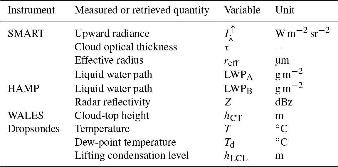
All instruments were pointed in the nadir direction and synchronized in time. However, the different fields of view (FOVs) of the instruments cause a systematic difference in the observed time series. All measured and retrieved quantities from SMART, HAMP, WALES, and the dropsondes are summarized in Table 1.
Table 1Measured and retrieved quantities from SMART, HAMP, WALES, and the dropsondes.
3.1 Spectral Modular Airborne Radiation measurement sysTem
During NARVAL-II, SMART measured the spectral upward and downward irradiance , as well as spectral upward radiance . Each quantity was recorded with two separate Zeiss grating spectrometers, one for the visible (Vis) range from 300 to 1000 nm wavelength and a second one for sampling the near-infrared (NIR) range from 900 to 2200 nm. By merging the spectra, about 97 % of the solar spectrum is covered (Bierwirth et al., 2009). The spectral resolution defined by the full width at half maximum is 2–3 nm for the Vis spectrometer and 8–10 nm for the NIR spectrometer.
The radiance optical inlet of SMART has an opening angle of 2∘. The sampling time tint was set to 0.5 s. For an average aircraft ground speed of about 220 m s−1 and a distance of 10 km between cloud top and the aircraft, this results in a FOV of about 100 m × 120 m for an individual pixel.
The optical inlets for and mainly consist of integrating spheres, which collect, direct, and scatter solar radiation from the upper or lower hemisphere. During NARVAL-II, the upward-looking inlet was equipped with an active stabilization platform to ensure horizontal alignment of the sensor, which is crucial as refers to a horizontal plane (Wendisch et al., 2001).
Prior to and after NARVAL-II, SMART was radiometrically calibrated in the laboratory using certified calibration standards traceable to the National Institute of Standards and Technology (NIST). A secondary calibration by a mobile standard was applied during the campaigns to track potential changes in the instrument sensitivity. The total measurement uncertainty of downward irradiance and upward radiance for typical conditions and observations of shallow cumulus is about 5.4 % for the Vis and 8.4 % for the NIR range, which are composed of individual errors due to spectral calibration, spectrometer noise and dark current, and primary radiometric calibration (Brückner et al., 2014).
3.2 HALO Microwave Package
HAMP is a combination of a passive microwave radiometer and an active cloud radar specifically designed for operation on HALO (Mech et al., 2014). The microwave radiometer includes 26 frequency channels between 22.24 and 183.31 GHz ± 12.5 GHz. The brightness temperature (BT) measured along the 22.24 and 183.31 GHz rotational water vapor lines provide the total column water vapor (Schnitt et al., 2017) and information on its vertical distribution. Liquid water emission increases roughly with the frequency squared. By combining BT in window channels, i.e., 31.4 and 90 GHz, mostly affected by liquid water with channels sensitive to water vapor, the LWP can be retrieved. This principle is also employed by satellite instruments that provide global climatologies of LWP, but suffer from the coarse footprint of a few tens of kilometers (Elsaesser et al., 2017).
The statistical LWP retrieval is based on a large variety of atmospheric profiles with differently structured warm clouds as training data composed from the dropsondes (Schnitt et al., 2017). Synthetic BTs are simulated from these profiles and subsequently used to fit a multiparameter linear regression model employing higher-order terms (Mech et al., 2007). Testing the retrieval algorithm on an independent subsample provides an accuracy of about 20 g m−2 for LWP values below 100 g m−2 and an accuracy of 20 % for LWP above (Jacob et al., 2019).
The cloud radar MIRA-36 operates at a frequency of 36 GHz and has a similar horizontal resolution as the LWP of about 1000 m and a temporal resolution of 1 s. Vertical profiles are divided into 30 m bins (Mech et al., 2014). The radar provides different parameters linked to the cloud microphysical properties, including the radar reflectivity Z, the linear depolarization, and the Doppler velocity, and the spectral width of the droplet size distribution. Note that the latter two are affected by the relative motion of the aircraft to the wind and the antenna width (Mech et al., 2014).
Radar reflectivity represents the sixth moment of the cloud droplet size distribution and is therefore strongly influenced by large droplets. In order to calculate the LWC, which is proportional to the third moment of the droplet size distribution (DSD), from Z, so-called Z–LWC relations are used, which are typically derived from in situ measurements. According to Khain et al. (2008), there is quite a lot of variability involved and as soon as the transition to drizzle sets in the relation can be off by orders of magnitude. Here the Z–LWC relation
following Frisch et al. (2000), is used to derive vertical profiles of LWC. With the binned LWCp at height gate p resulting from the vertical resolution of the radar, the LWP of the cloud is distributed by the weighting of Zp (Z at height gate p) and is the sum of the Z over all height gates at which a cloud was present. The techniques to derive brightness temperatures and radar reflectivity profiles are described in more detail by Konow et al. (2018a).
3.3 Water Vapour Lidar Experiment in Space (WALES)
The differential absorption lidar (DIAL) called WALES operates at four wavelengths near 935 nm to measure atmospheric water vapor. Mixing ratio profiles cover the whole atmosphere below the aircraft. WALES also contains channels for aerosol measurements at 532 and 1064 nm wavelengths with depolarization detection. At 532 nm, WALES uses the high-spectral-resolution technique, which distinguishes molecular from particle backscatter, to enable direct extinction measurements. Within this study only the aerosol channels are used to provide information on the cloud-top height. The ranging resolution of the instrument is 15 m. Together with the flight altitude inferred from the HALO onboard positioning system and an appropriate attitude correction, the accuracy of the cloud-top height detection is about 20 m.
The laser has a beam divergence of 1 mrad, which leads to an illuminated spot 10 m in diameter on the ground at a flight altitude of 10 km. Laser pulses are emitted with a repetition rate of 100 Hz; 20 signals are averaged to improve the signal-to-noise ratio, resulting in an along-flight-track resolution of 44 m at 200 m s−1 aircraft speed. Thus, the horizontal resolution is reduced compared to SMART and HAMP. Along track, this can be taken into account by further signal averaging.
Trade wind cumuli mostly appear randomly distributed with a tendency to form self-organizing structures (Bony et al., 2015). Typically, the vertical cloud extent is larger than the horizontal one within an individual cell. This is in contrast to stratiform cloud fields if common retrieval techniques to derive N are applied. Clouds smaller than the pixel size covered by the FOV bias the retrieval of microphysical properties (Oreopoulos and Davies, 1998a, b). The dominance of small-scale cumulus during NARVAL-II, ranging in the horizontal size of a few hundred meters, results in heterogeneous cloud scenes. This induces challenges with respect to cloud masking and RTS.
4.1 Cloud mask and precipitation flag
4.1.1 Cloud mask
To distinguish between cloud and cloud-free measurements over ocean surfaces, the difference in the spectral reflectivity is analyzed. The ratio χ of between 858 and 648 nm wavelengths is calculated in analogy to the MODIS cloud mask (Platnick et al., 2013) by
The cloud mask is based on the relative intensity of and χ. Therefore, a single measurement can be identified as cloudy when only a part of the SMART FOV with 100 m × 120 m is cloud covered. Masking each measurement point as cloudy or cloud free, the cloud length lcld is determined by counting the number n of consecutive cloud-masked measurements. Multiplied with the flight speed vac and the constant integration time of SMART of tint=0.5 s, the cloud length is calculated by
For vac≈220 m s−1 the smallest resolvable cloud size is in the range of 120 m along the flight track.
The length of trade wind cumulus can be shorter than the SMART FOV. To identify such cases, an additional homogeneity cloud flag (HCF) is introduced. The cloud is considered homogeneous (HCF is true) when a single observation is enclosed by five cloud-masked measurements. For clouds not surrounded by at least two cloudy pixels, the HCF is set to false. Therefore, the HCF identifies clouds that are large enough to fill the FOVs of SMART, HAMP, and WALES at the same time.
4.1.2 Precipitation flag
Precipitation is identified using the radar reflectivity Z. Measurements are considered to be affected by precipitation when Z exceeds a threshold of dBz within 50 to 200 m above sea level (Schnitt et al., 2017). This allows for the discrimination of precipitation events, which affect the LWP measured by the microwave radiometer and retrieved by SMART. The simple thresholding of radar reflectivity close to the sea surface might not capture all precipitating clouds as drizzle particles might evaporate before reaching the lower 200 m close to the sea surface.
4.2 Retrieval of cloud optical thickness and droplet effective radius
Based on the reflected solar radiance measured by SMART, a retrieval of τ and reff is performed by applying the radiance ratio method proposed by Werner et al. (2013). The use of radiance ratios at two different wavelengths reduces the uncertainties by the radiometric calibration of SMART. For the wavelength ratio applied here, an uncertainty of 6 % is assumed. Additionally, the use of ratios increases the retrieval sensitivity with respect to reff by clearly separating the dependence of on τ and reff and therefore the retrieval accuracy. Forward simulations of reflected spectral radiance were carried out with the libRadtran 2.0.2 package (Emde et al., 2016). The Fortran 77 discrete ordinate radiative transfer solver version 2.0 (FDISORT 2) after Stamnes et al. (2000) is used. The extraterrestrial is given by Gueymard (2004) and a marine aerosol profile after Shettle (1989) is selected. Vertical profiles of air temperature, pressure, and humidity are obtained from radiosondes released at the Bridgetown International Airport. For the optical properties of liquid water droplets, Mie calculations are performed.
The cloud optical thicknesses τ and reff are determined by a modified lookup table (LUT) method after Nakajima and King (1990). While τ is derived at 870 nm wavelength, reff is retrieved with the radiance ratio method using a ratio of measurements at 1050 and 1645 nm wavelengths. Compared to retrievals using larger wavelengths, e.g., 2.1 or 3.7 µm, reff retrieved by the SMART measurements represents not only the cloud particles at cloud top. The vertical weighting function for 1.6 µm also covers a significant amount of information from lower cloud layers (Platnick, 2000). Therefore, retrieved reff values are smaller than the actual cloud droplet size at CT, which are considered in Eq. (12) to calculate N. This leads to a systematic overestimation of N calculated from SMART measurements. Results from the SMART retrieval are denoted with the subscript “A”.
Clouds that do not cover the entire FOV of SMART bias the retrieved optical properties because they violate the assumption of plane-parallel clouds used in the RTS (Oreopoulos and Davies, 1998a, b). Lower values of bias τ towards lower values, whereas reff is shifted to larger droplet sizes (Cahalan et al., 1995). Further, the heterogeneous structure of trade wind cumulus is likely to cause 3-D radiative effects, like shadowing cloud areas by nearby cloud towers or enhanced reflectivity due to additional reflection into the FOV. These effects may also bias the retrieval of τ and reff and the calculation of N. Therefore, the HCF filter is applied to exclude measurements that are influenced by these processes. However, due to the low vertical extent of shallow trade wind cumuli that are analyzed here, these 3-D radiative effects are assumed to be negligible.
Liquid water path is obtained directly from libRadtran on the basis of τ and reff similar to Eq. (4). Liquid water path derived from SMART is again denoted with the subscript “A”. In the case of cloud heterogeneity, sun glint, or 3-D radiative effects, the retrieval of τ is very likely biased. Following Eq. (4), a bias of τ also influences the retrieval of reff and therefore LWP. To mitigate these effects, measurements of LWP from HAMP (denoted with the subscript “B”) are applied in the libRadtran radiation simulations of the cloud retrieval. Liquid water path data from microwave radiometers are obtained from wavelengths not influenced by sun glint or 3-D radiative effects. Using LWP from HAMP as a precondition, the LUTs reduce to one absorbing wavelength sensitive to reff. Therefore, the nonlinear dependence between τ and reff is removed and the retrieval becomes more reliable. Retrieved reff values from combined passive solar radiance and microwave measurements are denoted with the subscript “B”.
The retrieval of N from remote sensing observations is based on the relation proposed by Brenguier et al. (2000), which links N of a stratiform cloud to τ and reff by
The technique assumes an adiabatic vertical cloud profile, in which temperature linearly decreases and LWC linearly increases with height. An adiabatic profile implies that the total water mass mixing ratio of the cloud is conserved. This is true when (i) no water is removed from the cloud (no precipitation or fallout), (ii) no entrainment of drier air at the cloud edges occurs, and (iii) no evaporation from precipitation happens. As a result, the proposed method should be applied to nonprecipitating clouds only, which do not undergo strong vertical convection and mixing. A vertically constant N throughout the cloud layer is assumed. This assumption is verified for stratiform clouds and shallow trade wind cumulus by in situ measurements; e.g., Reid et al. (1999) and Wendisch and Keil (1999). The vertically constant N is mainly determined by the amount of available CCN at cloud base and their potential to form cloud droplets depending on the degree of supersaturation, which is controlled by temperature, entrainment of dry air, and updraft velocity.
The k parameter, relating the effective radius reff and the volumetric radius rvol, is set to k=0.8 for marine clouds following the suggestion by Martin et al. (1994) and Pontikis (1996). Depending on the cloud type the k parameter can vary by ±0.1 (Martin et al., 1994).
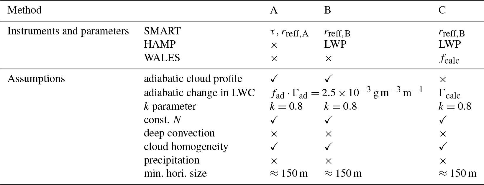
With the help of cloud properties retrieved by airborne remote sensing, Eq. (10) can be applied in different complexity to derive N. In the following three methods are proposed. Method A uses only SMART data, while method B additionally includes HAMP observations of LWP, and method C also involves measurements by WALES. The obtained parameters and applied assumptions are summarized in Table 2.
Table 2Overview of the cloud droplet number concentration retrievals and applied measurements, retrieval parameters, and assumptions.
5.1 Method A: based on cloud optical thickness and droplet effective radius
Method A follows the traditional satellite approach to feed Eq. (10) with τ and reff obtained by a single passive remote sensing instrument. Here, τA and rreff,A retrieved by SMART are applied. Using the radiance ratio retrieval of SMART to derive τ and reff,A from two infrared wavelengths, absolute calibration errors are reduced and the sensitivity on reff is increased. The degree of adiabacity is assumed to be 1. This implies that for trade wind cumuli, which are typically sub-adiabatic, the estimated N is potentially biased. However, similar retrieval assumptions are frequently applied to observations from satellites such as MODIS (Grosvenor et al., 2018b).
5.2 Method B: based on liquid water path and droplet effective radius
For adiabatic clouds, Eq. (4) can be solved analytically, which results in a relation that directly links LWP to τ and reff:
following (Brenguier et al., 2000). Equation (11) allows for the application of Eq. (10) with an independent measure of LWP instead of τ to calculate N. Combining Eqs. (10) and (11) leads to
In method B, LWP measurements by HAMP and derived reff,B from the combined SMART microwave–radiometer retrieval are applied. The results are denoted with NB. Exchanging reff,A by reff,B takes into account the fact that LWP is determined from HAMP only. This makes the retrieval independent of τ derived by SMART and therefore less sensitive to effects by sun glint. Further, LWP determination from HAMP applies wavelengths between 20 and 100 GHz, which are not influenced by aerosol particles. An additional advantage of the determination of LWP from HAMP is the separation of clouds for different LWPs and untangling the effects of varying LWP on α (McComiskey and Feingold, 2008).
5.3 Method C: based on liquid water path, droplet effective radius, and cloud geometric thickness
Equations (10) and (12) assume constant values of fad and Γad. Therefore, in method A and B the adiabatic profile of LWC follows the maximum theoretically possible profile under which liquid water is released due to condensation from upward motion in the atmosphere.
In situ measurements of stratocumulus and trade wind cumulus indicate that a majority of cloud profiles do not follow this adiabatic assumption (Wendisch and Keil, 1999; Merk et al., 2016). In most cases the profiles are sub-adiabatic, meaning a reduced increase in LWC with height, mostly due to entrainment and mixing from dry air at the cloud edges. When convection and mixing are moderate, an equilibrium between the droplets and the surrounding air can be assumed. Entrainment and mixing reduce fad but not necessarily N. Further, it might reduce the (super)saturation at the cloud edges, causing a shrinking of the droplets but not their complete vanishing. To account for a sub-adiabatic increase in LWC with height in method C, fad⋅Γad is replaced by observations. Observed Γcalc is determined by
with LWPB obtained by the microwave radiometer. The cloud geometric thickness is estimated from a combination of the WALES cloud-top height hCT observations and the lifting condensation level hLCL from dropsondes.
WALES can only derive hCT when the laser is attenuated by clouds with high τ. As a result, the lidar signal is attenuated soon and the cloud base height is not detectable. Therefore, hCB=hLCL is determined separately from dropsondes, which represent the large-scale thermodynamic structure of the atmosphere. Using the temperature T and dew-point temperature Td at the two lowermost points of the sounding, the lifting condensation level with is approximated (Espy, 1836). Nevertheless, uncertainties of estimated hLCL from dropsondes are in the range of ±35 m not considering additional uncertainties caused by the assumptions in the equation (Romps, 2017). Alternatively, cloud boundary determination by combinations of lidar, radar, and dropsonde are applied where (i) the cloud droplets are large enough to produce a detectable radar echo and (ii) no precipitation is present, but are complicated for heterogeneous cloud fields. Selection of the appropriate instrument synergy depends on the observed cloud scene. Utilization of radar observations is preferred, giving the best vertical resolution for well-defined cloud edges. Using the estimated Γcalc, Eq. (12) changes to
5.4 Simulated synthetic measurements
To systematically test the potential of the proposed synergistic retrieval methods, synthetic measurements of spectral upward radiance are created. In that way, the three different methods are compared, omitting the influence by measurement errors. Further, varying environmental conditions, like sea surface albedo, heterogeneous cloud conditions, and 3-D cloud radiative effects, do not influence the systematic comparison of the retrieval methods. The comparison is based on retrieved cloud droplet number concentration N with methods A, B, and C and Ncld calculated from the model clouds serving as the true value.
Six synthetic clouds are simulated. Their respective parameters are listed in Table 3. Cloud droplet number concentrations Ncld of 50, 100, and 200 cm−3 represent the typical range of pristine shallow trade wind cumulus (Siebert et al., 2013). For each Ncld an adiabatic and a sub-adiabatic cloud profile was set up. Cloud base height is 500 m and cloud-top height is 1000 m. For all cloud cases a linear increase in LWC and a constant Ncld with height are assumed. In the adiabatic cases (I, III, V) an LWP of 362 g m−2 and an adiabatic increase in LWC with height Γad of kg m−3 m−1, for a surface temperature of ≈30 ∘C, are used. For the sub-adiabatic cases (II, IV, VI) Γ is set to kg m−3 m−1, representing a cloud, which follows Γad by 60 % and leads to an LWP of 217 g m−2. To calculate the volumetric radius rvol(z), the cloud profiles are divided into 20 layers of equal thickness of 25 m. For each layer the parameterization of Martin et al. (1994) is applied:
In the radiative transfer model, the effective radius reff is used to determine the optical properties of the cloud particles instead of the volumetric radius rvol. To convert rvol(z) into reff(z) a k of 1.0 is applied, which considers the monodisperse droplet size distribution used in the model clouds. The synthetic measurements of are calculated with the same simulation setup as for the cloud retrieval described in Sect. 4.2.
Table 3Overview of all six synthetic cloud cases. The predefined cloud LWP and droplet number concentration N are denoted with the subscript “cld”. Cloud properties are calculated from the given cloud profile (subscript “lib”) and retrieved from synthetic spectral cloud reflectivities (subscript “R”). Calculated N is listed for all three methods: A, B, and C using the predefined cloud properties “lib” and the retrieval results from “R”.
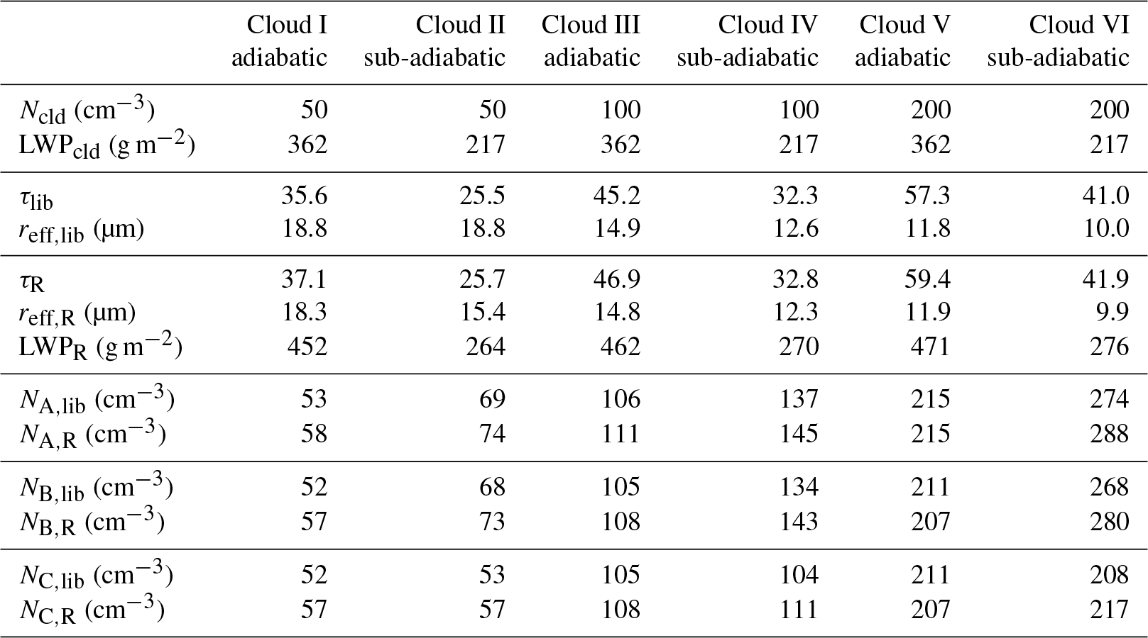
Simulated synthetic measurements of are applied to the retrieval method of τ, reff, and N of Sect. 5. All three methods (A, B, and C) are applied and results are denoted with the additional subscript “R”. The true values of τ from the RTS (subscript “lib”) are calculated directly from the given reff,lib, which represents the cloud-top reff of the model cloud. Total cloud optical thickness τlib and reff,lib from the libRadtran radiative transfer simulations are considered to be the reference values used to compare the retrieval results and the calculated N. For consistency the labeling of N for the three methods follows Sect. 5. An overview of all retrieved and calculated parameters is given in Table 3.
The retrieved cloud optical thickness τR is higher compared to the true value τlib for all cloud cases. The largest difference of 26 % is observed for cloud I. With increasing Ncld the absolute and relative differences become smaller. Systematically larger errors are found for the adiabatic clouds. A similar pattern is obtained for reff,R, which is always up to 2 % smaller than reff,lib. The sub-adiabatic clouds show the largest differences. The relative error decreases for higher Ncld. The systematic underestimation of reff,R, especially for the sub-adiabatic cases, with respect to reff,lib results from the penetration depth of the incident solar radiation into the cloud. For constant LWP, clouds with lower N have a lower τ, which reduces scattering. Therefore, the incident radiation can penetrate deeper into the cloud compared to clouds with higher N and τ (Platnick, 2000). As a result, is more influenced by lower cloud layers and the retrieved reff,R is systematically smaller than reff,lib. In this case, reff,R does not represent reff,lib at CT. The bias of reff,R from the reff,lib at CT feeds back into the retrieval of τR because of the dependence of τ and reff and the non-rectangular shape of the lookup table. The overall underestimation of retrieved reff,R, which appears for all passive remote sensing measurements based on reflected solar radiation, generally leads to an overestimation of N, which is intensively discussed, e.g., by Brenguier et al. (2000) and Grosvenor et al. (2018a, b), and therefore not repeated here.
Liquid water path LWPR is calculated with Eq. (11) from the retrieved τR and reff,R by assuming an adiabatic cloud profile. In all cases, the retrieval overestimates LWPR by 18 % for low Ncld up to 27 %. The deviation becomes larger for high Ncld.
The cloud droplet number concentration NA,lib is calculated with method A by using τlib, reff,lib and assuming an adiabatic vertical profile with Γad. This provides a reference for NA,R, which applies τR and reff,R. By comparing NA,lib and NA,R the influence of the remote sensing retrieval method (forward simulations and error due to penetration depth) on N for different Ncld becomes obvious. In general, NA,lib and NA,R of all clouds are larger compared to Ncld. Differences among NA,lib, NA,R, and Ncld result from smaller retrieved reff,R and higher τlib compared to τR. Another reason is the difference between Γad used in the model cloud and the assumed LWP parameterization in Eq. (11), which is applied in Eq. (10) to correlate LWP and τ. For all clouds, NA,R is larger than NA,lib and Ncld because in Eq. (10) N is dominated by and less sensitive to τ1∕2. Differences between NA,lib and NA,R vary between 0 % and 17 %, being largest for cloud I for which the deviation in reff,lib and reff,R is largest. The simulations also show that NA,lib and NA,R are largest for the sub-adiabatic cloud cases.
For method B, NB,lib and NB,R are larger than Ncld with smaller differences for the reference values of NB,lib and larger differences of NB,R compared to Ncld. For method B the deviations of NB,lib and NB,R compared to Ncld are largest for the sub-adiabatic cloud cases. The systematic overestimation of NB,R for all clouds is due to the lower reff,R. The differences are reduced for increasing Ncld because the differences between reff,R and reff,lib decrease. This clearly shows that a wrong estimation of reff influences the calculation of N most significantly, while τ contributes to a minor part only, independently of which method is used. These results allow for the conclusion that reff must be retrieved close to cloud top. This is possible if the retrieval applies an appropriate wavelength in the infrared, whereby radiation is effectively absorbed within the uppermost part of the cloud. Otherwise, systematic overestimation of N occurs.
By applying method C the sub-adiabatic nature of the cloud profiles (II, IV, VI) is considered in the estimation of N. The calculated Γcalc is assumed to be correct and identical to the profile of the constructed clouds, with fad=0.6 and . Therefore, it is obvious that N values calculated from method B and C are also identical for adiabatic clouds. In general, NC,R derived from method C is closer to Ncld than NB,R. However, for the sub-adiabatic clouds (II, IV, VI) the results for methods B and C differ. Cloud droplet number concentration NC,lib is closest to N for all cloud cases and methods. The same pattern is present for NC,R with the best agreement to Ncld compared to method A and B. Deviations in NC,lib and NC,R to Ncld are reduced with increasing N. This shows that a correct assumption of Γcalc, as possible with method C, is crucial for a reliable calculation of N and can compensate for biases in N that result from the sub-adiabatic cloud profile.
5.5 Calculation of retrieval uncertainty of cloud droplet number concentration
Cloud droplet number concentrations calculated with Eqs. (10), (12), and (14) are mainly affected by uncertainties from τ, LWP, and especially reff, but also depend on the accuracy of k, fad, and Γad. To estimate the uncertainties of retrieved N, it is assumed that the errors are normally distributed and independent from each other. In this case the uncertainty of NA from Eq. (10) is calculated by
and analogous for Eqs. (12) and (14). All uncertainties of N presented in the following sections are based on calculations with this approach. The uncertainties of the single parameters assumed in the calculations are summarized below.
For method A, B, and C, the uncertainty of k, representing the shape of the droplet size distribution, is set to according to the range of values suggested by Martin et al. (1994) and Pontikis and Hicks (1992).
For methods A and B the degree of adiabacity fad is fixed to 1. In that case, no uncertainty in a measurement scene is attributed to fad. For method C, the uncertainty of fcalc is determined by the uncertainty of hCT, hCB, and retrieved LWP following Eq. (13). Cloud-top height from WALES is determined with an accuracy of m. The cloud base height is derived from single dropsondes and therefore prone to horizontal variability in T, p, and Td. Based on an analysis of different dropsondes in close vicinity, a cloud base height hLCL=660 m ± 35 m is assumed. The evaluation of all dropsondes shows that the thermodynamic conditions in the selected area stayed constant (ΔT<2 K and Δp<4 hPa) during the flight time with hCT≈1800 m, TCT=20.2 ∘C, and pCT=820 hPa. The accuracy of the deployed Vaisala dropsondes RD94 is reported to be within K and hPa. Uncertainties of NC caused by errors in Γad are therefore negligible compared to the influence of τ and reff.
The adiabatic increase in LWC with height calculated from the Clausius–Clapeyron equation depends mostly on cloud-top temperature TCT and to a lesser degree on cloud-top pressure pCT. Therefore, Γad depends on TCT and pCT, too. The cloud droplet number concentration is mostly affected by the assumed TCT, whereby pCT makes only a minor contribution. Despite that, the cloud-top pressure more strongly affects warm than cold clouds (Grosvenor et al., 2018b). For the uncertainty calculation, a temperature difference of 2 K is considered, which changes Γad by g m−3 m−1 for the reference value of g m−3 m−1.
The uncertainty of the retrieval of τ and reff,A results from the measurement uncertainties of SMART, which are described in Sect. 3.1. For typical trade wind cumulus, uncertainties of ±0.1 for τ and ±1.1 µm for reff,A are assumed.
Small clouds not covering the entire FOV bias the retrieval of the optical properties towards low τ, large reff, and resulting low N. Additionally, the uncertainties in reff increase for low τ. Correlation of τ and Δreff reveals that this effect is pounced for τ≤5. This mostly results from the increasing influence of the ocean surface with low albedo in broken cloud regions.
From the error estimation of the N retrieval it can be concluded that uncertainties in reff, LWP, and H have to be minimized as they influence the retrieval the most. Determination of hCB, either from the dropsondes or the radar, and resulting H have to be accurate within at least ±60 m.
In addition to the measurement uncertainties, the sensitivities of the individual retrievals on τ, reff, LWP, hCT, and hCB have to be considered. The retrieval of LWP by SMART is sensitive for thin clouds (LWP<100 g m−2) with an increasing uncertainty for optically thicker clouds caused by a reduced response of reflected I↑ in the case of high optical thickness. The usage of LWP from SMART for optical thin clouds is further supported by the retrieval uncertainty in LWP by HAMP for LWP values below 100 g m−2. For clouds with LWP around 100 g m−2, both methods A and B (assuming an uncertainty of LWP derived by HAMP of about 20 %) lead to an uncertainty of N in the range of 10 cm−3. In the case of thicker clouds (LWP>100 g m−2), method B with LWP from HAMP is used, achieving N accuracy of ±14 cm−3 from SMART. For clouds with LWP>100 g m−2 and considerable geometric thickness (H>1500 m), HAMP-retrieved LWP becomes more representative as the retrieval represents the entire cloud and not only the CT properties observed by SMART. Common satellite-based microwave radiometer retrievals of LWP above 180 g m−2 are error-prone because of their large footprint. With the smaller footprint of HAMP these uncertainties in LWP are reduced, resulting in a lower uncertainty in retrieved NB and NC.
The retrievals of reff,B from combined measurements of SMART and HAMP are slightly more prone to uncertainty of the LWPB measurements and lead to uncertainties of reff,B of up to ±1.5 µm, being sightly higher than reff estimated for method A. However, the uncertainty of N with respect to reff is lower, as the sensitivity of NB with respect to reff,B is lower in Eq. (12) compared to Eq. (10). The sensitivity study leads to the conclusion that an appropriate retrieval of reff is the most important factor for the calculation of N.
For the exemplary ideal adiabatic case study discussed above, the total uncertainties of the three methods are cm−3, cm−3, and cm−3. For sub-adiabatic clouds, the uncertainties of method A and B increase due to the assumption of adiabaticity. The additional error in N results from the increased variability in fad.
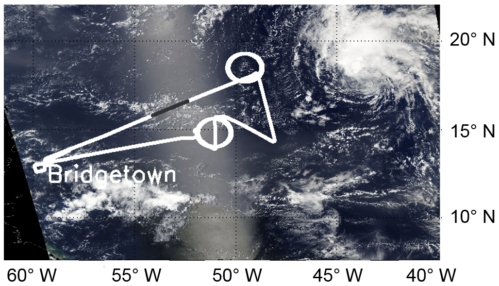
Figure 2Flight track of HALO (white) from RF 06 (19 August 2016) plotted on a MODIS Terra satellite image from 19:30 UTC. The section for which the remote sensing measurements are analyzed (19:24 to 19:39 UTC) crosses a region with aggregated trade wind cumulus and is plotted in gray.
The retrieval of N is applied to two measurement cases observed during NARVAL-II. Figure 2 shows the flight track (white) of Research Flight 06 (RF 06) from 19 August 2016 and the flight section (19:24 to 19:39 UTC) of the track for which the remote sensing measurements are analyzed. The satellite image represents the cloud situation at 19:30 UTC. The presence of intense sun glint is visible, which enhances the reflected radiance and influences the cloud detection (low contrast) and the retrieval of τ and reff,A. The analyzed time period is divided into two parts, cloud case no. 1 and cloud case no. 2. The northeastern part of the flight track (19:29–19:32 UTC) was dominated by aggregated trade wind cumuli, whereas in the southwestern part (19:32–19:36 UTC) shallow cumuli were present. The general weather situation was characterized by moderate convection with low cloud-top altitudes. Locally, more dense cloud fields formed at about 10 and 16∘ N at 55∘ W.
Time series of measured and retrieved parameters of both cloud cases are shown in Figs. 3 and 4. The three methods to calculate N assume that there is no precipitation present. Because measured Z is most sensitive to large cloud droplets, it cannot be guaranteed that drizzle is excluded completely. Estimation of the drizzle rate on the basis of H and N as proposed by Pawlowska and Brenguier (2003) and vanZanten et al. (2005) is not possible as retrieved N is biased by the process of drizzle formation and therefore not applicable with the presented instrument setup of HALO. Flight sections flagged for precipitation are highlighted by gray boxes. At the top of Figs. 3 and 4 the cloud mask (blue) and the homogeneity cloud flag HCF (yellow) are indicated. Images of RGB composites by specMACS are given in the lower part of the plots to illustrate the visual cloud characteristics. Data gaps are due to cloud-free pixels.
6.1 Cloud case no. 1
Case no. 1 represents a stratiform single-layer cloud without any convective areas, which is an ideal test case for the N retrieval. The cloud optical thickness τ shown in Fig. 3a is generally low and ranges between 0 and 2 at the beginning of the section, while τ increases to up to 6 with time. The uncertainty of τ is estimated to be ±0.1. The effective radius reff,A (panel b, black line) ranges between 9.6 and 26.3 µm with an uncertainty of ±1.0 µm, while reff,B is between 8.3 and 30 µm retrieved with a slightly higher uncertainty of ±1.5 µm. For the first cloud part, the SMART liquid water path LWPA (panel c) is calculated with Eq. (4) using retrieved τ and reff,A. For the first part of the cloud LWPA is slightly lower than the LWPB measured by the microwave profiler, while with increasing τ the agreement between the two LWPs improves. Vertical profiles of LWC shown in Fig. 3g are below the detection threshold except for four cloud patches. This indicates that no precipitation was detected, but slight drizzle cannot be excluded. Cloud base height is estimated from dropsondes to be around 1500 m, while hCT is determined by WALES. The resulting cloud geometric thickness H (Fig. 3d) varies between 100 and 420 m. Cloud adiabaticity fcalc (Fig. 3e) is mostly below 0.5, indicating a considerable sub-adiabatic cloud. Calculated NA and NB are shown in Fig. 3f and range between 5 and 40 cm−3, which results from the low τ and LWPB and the large reff,A and reff,B. The cloud droplet number concentration NA shows a peak around 19:34:30 UTC and NA at 19:35:00 UTC. Cloud droplet number concentration NC derived by method C is lower than NA and NB and does show a reduced variability compared to NA and NB. However, the uncertainty of all N is about ±15 cm−1. While in the first part of cloud case no. 1 the differences in N are large, there is a good agreement among all three methods in the second part, for which all results are inside the uncertainty range of each method. Mean values of measured and retrieved parameters for cloud case no. 1 are listed in Table 4.
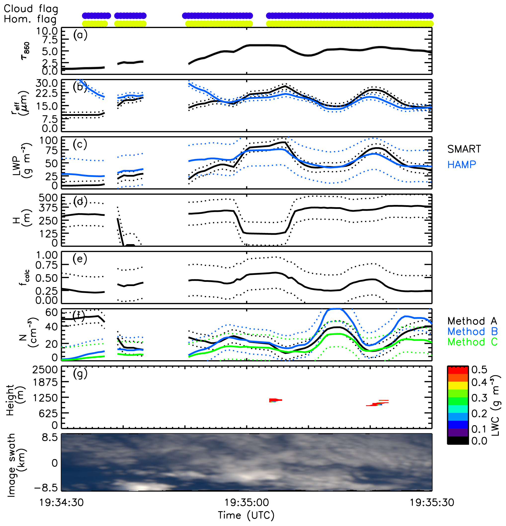
Figure 3Time series of measured and retrieved cloud properties for cloud case no. 1 from 19:34:30 to 19:35:30 UTC of RF 06. Cloud droplet number concentration N is shown for all three methods (A, B, and C). Uncertainty ranges of the individual parameters are indicated by dotted lines. At the top, the cloud mask (blue) and the homogeneity cloud flag (HCF) (yellow) derived by SMART are indicated.
6.2 Cloud case no. 2
The second case represents a more heterogeneous single-layer cloud observed between 19:29 and 19:32 UTC, shown in Fig. 4. This cloud is in a later state of development and shows moderate convection with slight precipitation. In these areas (highlighted in gray), the criteria for cloud homogeneity are not fulfilled. Despite that and the slight precipitation, calculation of N is performed, knowing that the retrieval of N using method A and B is prone to errors under these circumstances. These results are used to evaluate the improvement of retrieved N by method C, which accounts for cloud geometry and sub-adiabacity. By comparing convective and non-convective areas of cloud case no. 2, the limitations and advantages of the three methods are investigated. Mean values of the measured and retrieved parameters from the three different methods, separated for nonprecipitation and precipitation, are summarized in Table 4.
For the nonprecipitating and homogeneous part of cloud case no. 2, τ does not exceed a value of 30 and reff,A and reff,B range between 18 and 40 µm (Fig. 4a, b). The uncertainty of all measured and retrieved parameters is in a similar range as calculated for cloud case no. 1. Retrieved LWP from SMART and HAMP (Fig. 4c) agrees within the uncertainty range of HAMP for most parts of the homogeneous cloud sections. Larger differences appear around 19:29:30 UTC when LWPA is larger than LWPB. For method C, cloud geometrical thickness H is calculated from a combination of HAMP and WALES. Radar reflectivity Z is above the precipitation detection threshold of −20 dBZ and allows for the determination of vertical profiles of the LWC and hCB with an average value of hCB≈900 m when no precipitation is present. Cloud-top height hCT from WALES ranges between 200 and 1000 m for the nonprecipitating regions. This results in a highly variable fcalc, which varies strongly between 0.05 and 1.0.
Cloud droplet number concentrations from method A and B calculated for cloud case no. 2 are generally low (see also Table 4), mostly ranging between 20 and 40 cm−3. Together with large reff,A and reff,B these values indicate typical pristine maritime clouds. An exception is observed around 19:29:30 UTC when N peaks up to 120 cm−3 for all three methods mostly resulting from a decrease in reff,A and an increase in τ. The decrease in reff might result from 3-D radiative effects at the cloud edge overestimating the cloud particle size and could have biased the retrieval of N.
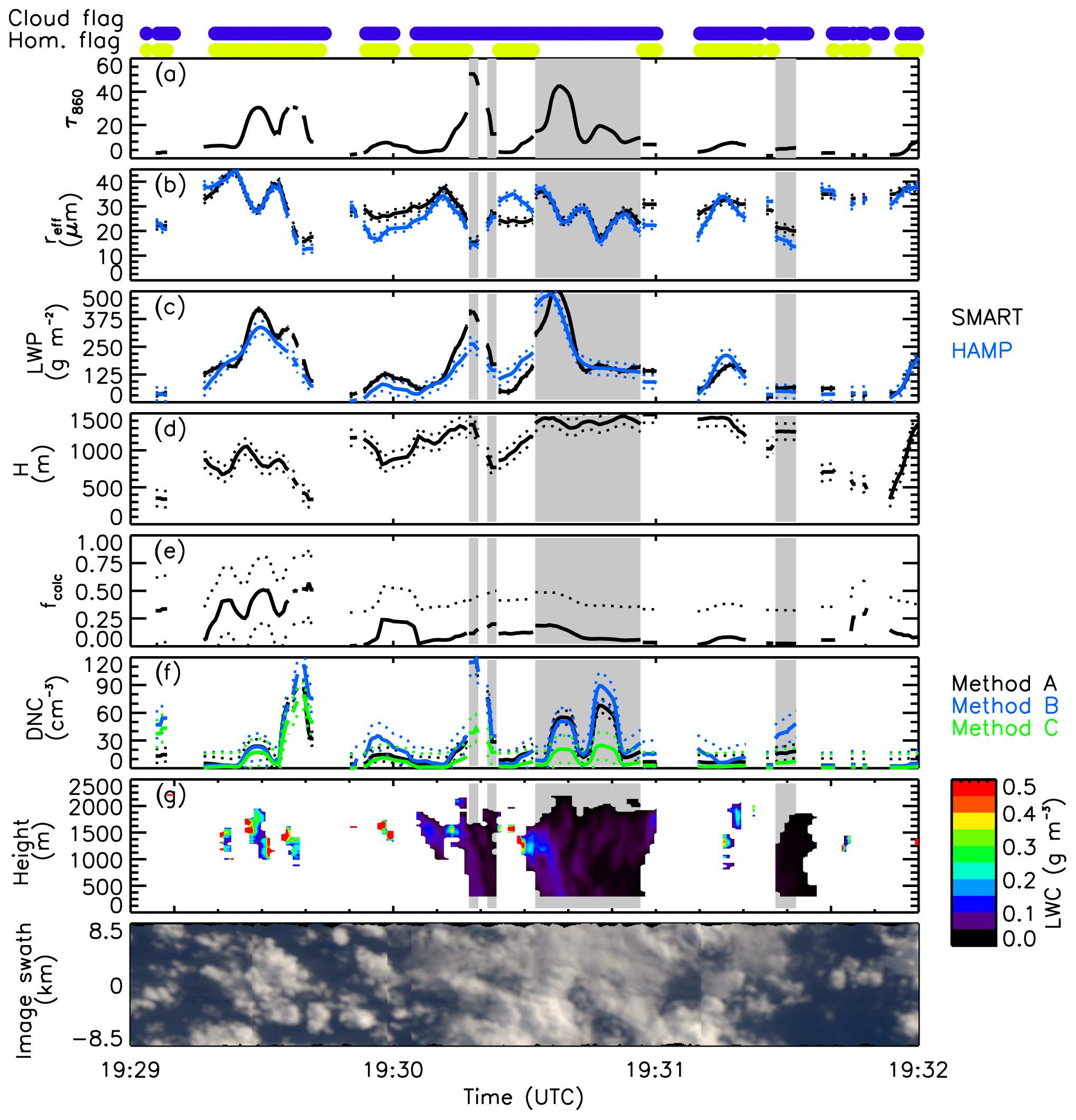
Figure 4Time series of measured and retrieved cloud properties for cloud case no. 1 from 19:29 to 19:32 UTC of RF 06. Cloud droplet number concentration N is shown for all three methods (A, B, and C). Uncertainty ranges of the individual parameters are indicated by dotted lines. At the top, the cloud mask (blue) and the homogeneity cloud flag (HCF) (yellow) derived by SMART are indicated.
In the areas marked with precipitation, retrieved τ, LWPA, and LWPB are higher compared to the precipitation-free regions, while reff,A and reff,B are in the same range as for the nonprecipitating areas. In contrast to the homogeneous parts of the cloud, the convective regions show stronger horizontal heterogeneity in all parameters. The optical thickness reaches up to 40 and rreff,A ranges from 20 to 38 µm. In these areas the LWPB from HAMP exceeds 270 g m−2 and shows a maximum value up to 500 g m−2. Liquid water path from SMART is in the same range of LWPB except for the first precipitation section (19:30:30 UTC) in which LWPB is lower than LWPA. For the precipitating regions hCB is assumed to be at the same level as determined for the nonprecipitating regions, as precipitation makes the cloud base invisible for the radar. The cloud geometric thickness H is slightly higher for the connective regions and ranges between 800 and 1300 m. The calculated adiabaticity fcalc is lower than 0.5 for the majority of the measurement and shows that most parts of the cloud are sub-adiabatic. For the precipitation regions calculated N values are between 10 and 90 cm−3, with the highest concentrations for method B, followed by method A and the lowest N for method C. In the areas with precipitation, N shows a systematically higher variability observed by all three methods and likely caused by the variability of reff retrieved from SMART. One reason for this variability is the relation of rvol to rreff, which is assumed to be (i) constant in the retrieval of reff,A and reff,B and (ii) significantly influenced by the formation of precipitation. Therefore, calculated N values by all three methods are highly prone to errors for precipitating clouds. The variability of N might also be caused by intense turbulent mixing processes within the cloud. Concluding from that, it is suggested to filter areas with stronger convection, precipitation, and heterogeneous scenes and analyze the retrieved N with special care.
Table 4Mean values of cloud properties for cloud cases no. 1 and no. 2.
6.3 Statistical analysis of liquid water path, droplet effective radius, and number concentration
Statistics of retrieved cloud properties are analyzed for measurements between 19:24:00 and 19:39:00 UTC only, when the HCF indicates homogeneous clouds and uncertainties of the retrieved cloud parameters are low. An extension of the analysis to other flights is not possible yet because the reliable application of the retrieval of N requires careful data selection and good quality data from all individual instruments. However, in total 700 individual measurements are included, which represents a cloud field 77 km in length. The clouds were separated into precipitating (p) and nonprecipitating (np) pixels. Mean values of the parameters for each measurement are summarized in Table 4.
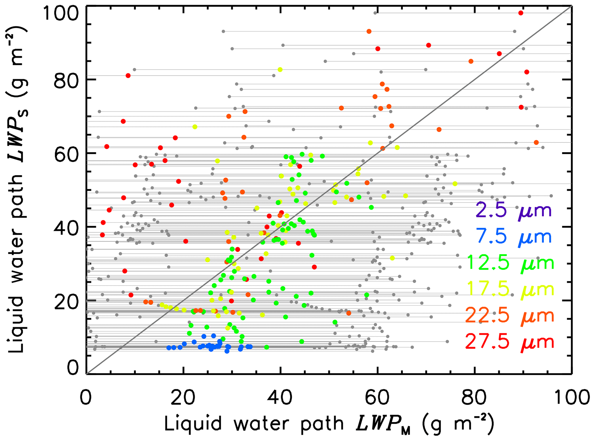
Figure 5Comparison of liquid water path LWPB from HAMP microwave radiometer and LWPA calculated from τ and reff,A retrieved by SMART. The color code indicates different ranges of reff,A. HAMP uncertainties of LWP (±30 g m−2) are indicated by gray errors bars.
Figure 5 compares measurements of LWPA and LWPB. The data are separated for different reff,A split into bins of 5 µm size. For the selected time period, LWPA agrees with LWPB within the uncertainty range of HAMP of ±30 g m−2 indicated by the gray error bars. The differences of LWPA and LWPB show a larger variability for clouds with large reff,A than for clouds with small reff,A. For larger cloud droplets, the retrieval uncertainty of τ and reff,A increases, as does LWPA derived from SMART. Additionally, SMART has a higher sensitivity to droplets at cloud top and the FOV of HAMP is slightly larger compared to SMART, which can explain some of the observed variability. Slightly different viewing directions have to be considered, too. While for SMART the LWPA is calculated assuming an adiabatic profile with the retrieved reff,A representing cloud top, HAMP obtains an integrated measure of LWP, whereby all cloud layers are more homogeneously weighted and no assumption on the cloud profiles is required. Therefore, a difference between LWPA and LWPB indicates that the observed clouds are nonadiabatic. For LWPA>LWPB less liquid water is at CB than predicted by adiabatic theory and clouds are sub-adiabatic. For LWPA<LWPB liquid water at CT is reduced, likely by precipitation as supported by the preferred reff in these LWP regimes (Fig. 5).
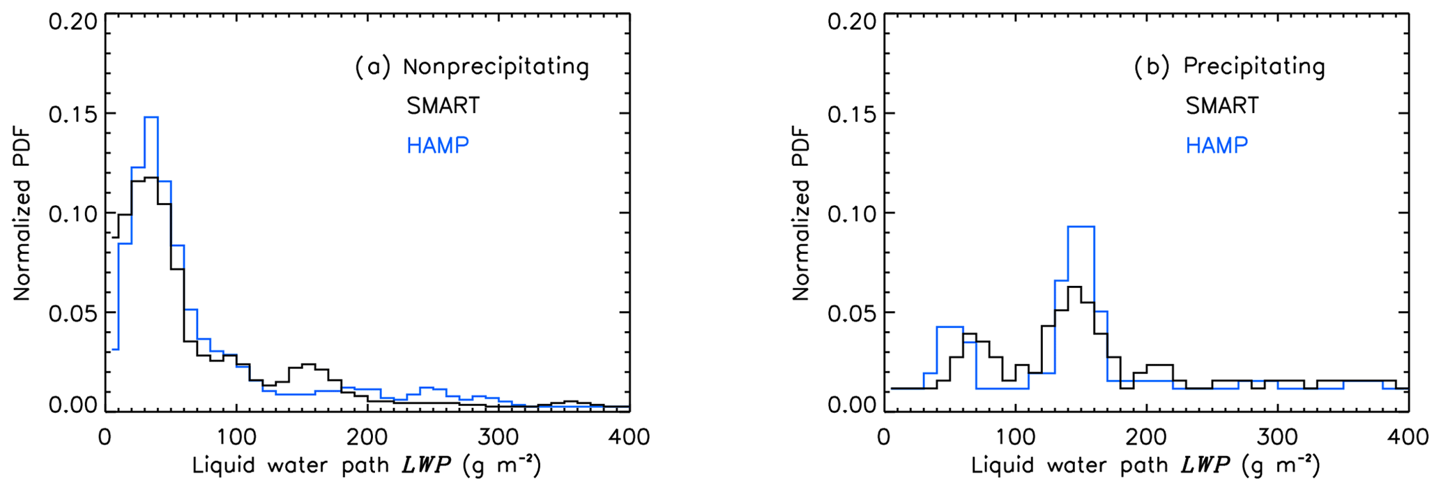
Figure 6Normalized probability density function (PDF) of measured and calculated LWP from HAMP (blue) and SMART (black). Distributions are filtered for nonprecipitating (a) and precipitating (b) clouds.
Figure 6a and b show the normalized probability density function (PDF) of LWP retrieved by HAMP and SMART separated for precipitating and nonprecipitating clouds. For the nonprecipitating clouds, the distributions of LWP retrieved by SMART and HAMP are dominated by clouds below 100 g m−2. Higher LWPs are obtained for regions with precipitation, for which the distribution is shifted towards larger values of LWP. The PDFs of LWPA and LWPB show a dominant mode at around 150 g m−2. A second smaller mode is present for LWPA at 80 g m−2 and LWPB at 50 g m−2 for both instruments. The agreement of the LWP retrievals, utilizing reflected solar radiation from CT (method A) and passive microwave measurements (method B), indicate that the cloud microphysical properties are sufficiently determined by the SMART retrieval, despite the assumption of an adiabatic cloud profile in method A.
Table 5Measured and retrieved properties in the entire period for both cloud cases, separated for precipitating (p) and nonprecipitating (np) clouds.

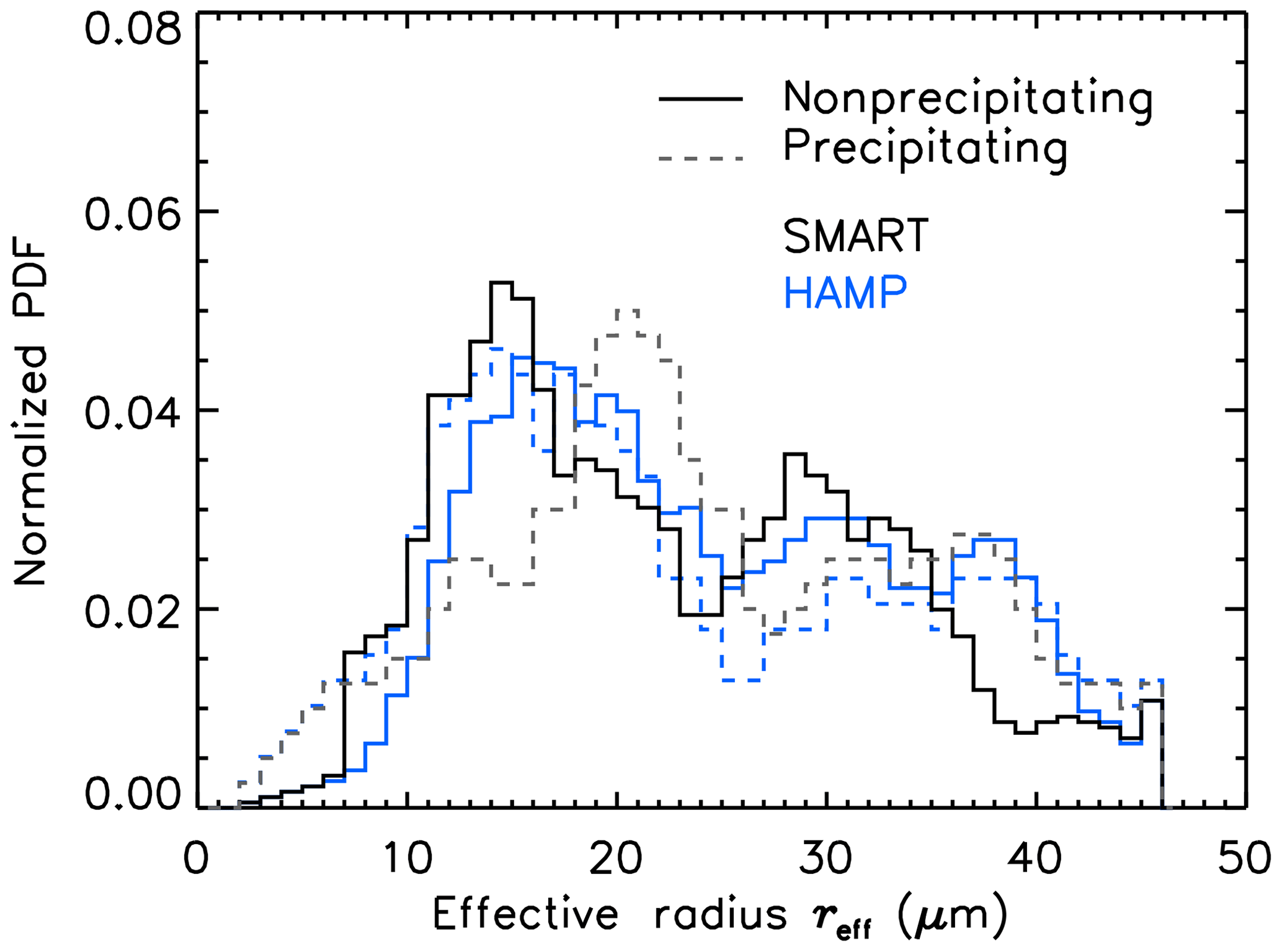
Figure 7Normalized PDF of the effective radius reff,A retrieved by using the ratio of 1645 to 1050 nm in black and reff,B from the combined spectrometer–microwave retrieval in blue. Distributions are filtered for nonprecipitating (solid line) and precipitating (dashed line) clouds.
In Fig. 7 the normalized PDFs of reff,A retrieved from SMART only (method A) and reff,B retrieved synergistically from SMART and HAMP (method B) separated for precipitating and nonprecipitating clouds are presented. The mean value for nonprecipitating clouds is around µm and the median is at µm. This droplet size range agrees with in situ measurements of pristine trade wind cumulus by Siebert et al. (2013) and remote sensing measurements by Werner et al. (2014) in the same geographic region. The distribution shows a bimodal structure with a first mode around 15 µm and a second mode around 32 µm. The PDF of reff,A for precipitation situations shows a similar structure being shifted towards larger reff,A with values of µm and µm. The first mode is at 21 µm and the second mode is at 36 µm. The PDFs of reff,B for the np clouds are shifted to larger values by approximately 3 µm, additionally showing a third mode around 38 µm. In contrast, the PDF for the p clouds is shifted to lower values by up to 8 µm and showing only the bimodal structure with peaks around 15 and 33 µm.
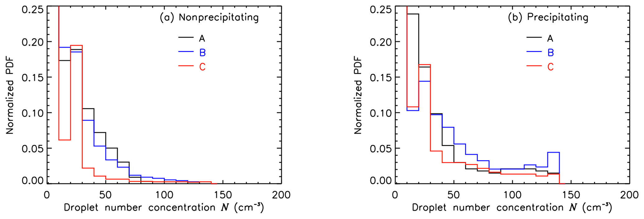
Figure 8Normalized probability density function of the cloud droplet number concentration N for the selected flight path using method A, B, and C. Distributions are filtered for nonprecipitating (a) and precipitating (b) clouds.
Figure 8a and b show normalized PDFs of the calculated N for nonprecipitating (panel a) and precipitating regions (panel b) of the selected flight leg from all three methods (A, B, and C). For nonprecipitating clouds (Fig. 8a) the distribution of NA peaks at NA≈30 cm−3 with a steep decrease towards a concentration of ≈100 cm−3. The first local maximum of the NB distribution is at NB≈30 cm−3, slowly decreasing for larger N. Only a slight difference between NA and NB is present for higher NA. This can be explained by the slightly higher values of SMART LWPA compared to HAMP LWPB. The PDFs of NA and NB show reasonable results for pristine, maritime clouds with relatively large reff,A and accordingly low N from method A and B. Cloud droplet number concentrations from method C are significantly lower as a result of the considered adiabaticity of the individual clouds.
Measurements affected by precipitation compared to Fig. 8a show almost the same distribution with a shift to larger N for all three calculation methods, especially for method C. Filtering for precipitating clouds, the statistics might be biased by only considering further developed clouds in which precipitation formation changes and broadens the droplet size distribution. This leads to differences in the means of rvol and reff, influencing the k parameter, which is assumed to be 0.8 in the N calculation.
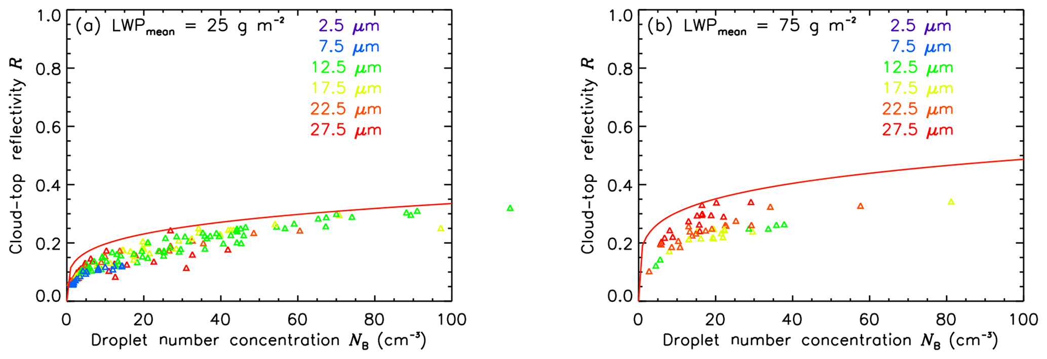
Figure 9Cloud-top reflectivity ℛ532 as a function of cloud droplet number concentration NB for homogeneous, nonprecipitating clouds of different liquid water paths LWPB (a: 0–50 g m−2, b: 50–100 g m−2). The droplet effective radius reff of each measurement is indicated by the color code. The red line represents simulated reflectivity ℛ532 from radiative transfer calculations for clouds with the same LWP.
Figure 9 shows the cloud-top reflectivity ℛ532 measured by SMART at 532 nm as a function of NB retrieved from combined SMART and HAMP measurements. Only measurements of the flight leg during which no precipitation was observed are presented. The data are binned for two different LWPs. Figure 9a shows clouds with LWP between 0 and 50 g m−2, and Fig. 9b shows clouds in the range between 50 and 100 g m−2. Colors represent reff,B binned from 5 to 30 µm in 5 µm steps (label in Fig. 9 refers to the mean bin value). Using ℛ532 as a measure for the reflectivity of the cloud, the sensitivity of ℛ532 to changes in N is comparable to the model-based sensitivity study in Sect. 2. Therefore, in Fig. 9 radiative transfer simulations of theoretical ℛ532,sim for clouds of the same LWP are added by the red line. For the thin clouds in Fig. 9a the measured ℛ532 shows a clear increase for higher NB over the entire measurement range. This correlation is less pronounced for the thicker clouds in Fig. 9b due to a reduced range of ℛ532 and N, and the observations may not cover the entire natural variability. However, for both cloud subsamples, the measurements follow the theoretical line given by the simulations and the measured ℛ532 values are too low or retrieved N too high. Both might be attributed to measurement biases: either the radiometric calibration of SMART or the retrieved LWPB and reff,B, which feed the calculation of NB. Additionally, the homogeneous assumption of cloud properties applied in the RTS can lead to an overestimation of ℛ532,sim compared to the measurements. The subdivision of data for different reff,B shows that clouds in an early developing state with low LWPB (Fig. 9a) are dominated by smaller cloud droplets up to µm, whereas clouds in a later development state with higher LWPB (Fig. 9b) are dominated by cloud droplets larger than µm.
Trade wind cumuli are a ubiquitous cloud type in the tropics influencing the Earth radiative energy budget significantly. In spite of their importance, they are not appropriately represented in numerical weather prediction (NWP) and global climate models (GCMs), causing considerable uncertainties in the radiation schemes of the models. Platnick and Twomey (1994) showed that the cloud-top albedo α of clouds with low cloud droplet number concentration N and low liquid water path (LWP), such as trade wind cumuli, respond sensitively to changes in N. In order to obtain improved parameterizations and global distributions of N, several methods, including active and passive remote sensing from the ground and satellites, are developed, but no operational products are available yet. Only a limited number of field campaigns with in situ measurements of selected cloud cases exist. As a result, the natural variability of trade wind cumulus is poorly covered by appropriate measurements.
Sensitivity simulations in this paper show that shallow trade wind cumuli with LWP below 200 g m−2 and N below 100 cm−3 are very sensitive to changes in N. In the case of an LWP of 75 g m−2, an increase in N from 50 to 100 cm−3 leads to an increase in α by 0.1. Therefore, the influence of trade wind cumuli on the Earth radiation energy budget is variable and significantly depends on the interaction among α, N, cloud optical thickness τ, cloud droplet effective radius reff, and different thermodynamic conditions (e.g., varying LWP), which has to be investigated systematically.
Applying the common satellite retrieval techniques of N to measurements conducted with a high-flying aircraft, such as HALO, shows the potential of combined airborne passive and active remote sensing instruments. Using aircraft instead of satellite platforms allows for the investigation of specific cloud types under selected atmospheric conditions, e.g., cloud-top temperature TCT, cloud-top pressure pCT, and LWP.
This was done during the second campaign of NARVAL-II, for which HALO was equipped with a set of passive and active remote sensing instruments. The SMART measured upward and downward spectral irradiance and upward radiance , which enables the calculation of α and retrieval of τ and reff,A at cloud top. The HAMP enables the performance retrievals of LWP and radar reflectivity Z used to separate for bins of LWP and to discriminate between nonprecipitating and precipitating cloud sections. Combining measured values of by SMART and LWP by HAMP, alternative values of reff are retrieved, which are less influenced by 3-D cloud radiative effects. Cloud-top height hCT is determined by the WALES, while the cloud base height hCB is estimated from dropsondes or radar data.
The heterogeneity of shallow trade wind cumulus fields during NARVAL-II has to be considered in the analysis. This is especially important in the retrieval of τ, reff, and N at the average flight speed of HALO (vac≈220 m s−1) and different instrument FOVs, being in the size range of individual clouds. The heterogeneity is indicated by the high occurrence (63 %) of clouds with a horizontal size smaller than 300 m. In this context, careful cloud masking and filtering for homogeneous cloud regions is crucial. Using cloud flagging and masking, the calculation of N can be applied to approximately 55 % of all observed clouds.
Three different methods to retrieve N based on Eq. (10) are presented and the application is shown for synthetic measurements of six different clouds with Ncld of 50, 100, and 200 cm−3, each following an adiabatic and sub-adiabatic cloud profile. From the synthetic measurements it can be concluded that the calculation of N on the basis of τ and reff,A from SMART method A is suggested for optically thin clouds (LWP<100 g m−2), while for optically thicker clouds method B is preferred, whereby τ is replaced by LWP retrieved by HAMP. For homogeneous clouds when the cloud boundaries can be determined precisely from active radar, lidar, and dropsonde measurements, the resulting calculated adiabaticity factor Γcalc can be determined and used as a correction factor in the calculation of N as the optimal case (method C). The synthetic measurements further showed that the differences between modeled Ncld and retrieved NC,lib or NC,R with method C are significantly reduced compared to method A or B for all three cloud cases. This indicates that a correction with Γcalc is vital and necessary for the calculation of N of shallow trade wind cumuli using remote sensing techniques. Otherwise, a systematic overestimation of retrieved N is present and measurements are not feasible.
Subsequently, the three methods are applied to a homogeneous and a heterogeneous cloud section. Both cloud cases are statistically analyzed. Determination of the cloud geometric thickness H was relatively uncertain in both cases and method C was excluded from the statistical analysis. Probability density functions of LWP, reff, and N for the two cloud scenes are presented. Correlations of cloud-top reflectivity ℛ532 at 532 nm to NB for two binned LWPB cases are shown. These are used to validate modeled ℛ532, to describe the sensitivity of ℛ532 with respect to N, and allow for the parameterization of the Twomey effect. Comparison of simulated and measured ℛ532 showed systematically lower values of observed ℛ532. Further testing of the proposed method on longer flight sections is necessary to cover the natural variability of trade wind cumuli and thermodynamic conditions. Despite remaining uncertainties and assumptions, the application of Γcalc, the separation for different LWPs, and the smaller FOV of all instruments allow for the better investigation of cloud–radiation interactions compared to large-scale averaged satellite measurements.
The data products of SMART, HAMP, and WALES of the NARVAL-II campaign are available at the HALO database (https://doi.org/10.17616/R39Q0T, Deutsches Zentrum für Luft- und Raumfahrt, 2019). For access to the data and information, please contact the corresponding author or the responsible coauthor. Calibrated and quality controlled data from HAMP are accessible at https://doi.org/10.1594/WDCC/HALO_measurements_3 (Konow et al., 2018b).

KW developed the proposed method and drafted the paper. MW and AE prepared the field campaign and contributed to the final version of the paper. SC and MJ added annotations concerning microwave and radar data, and MWirth provided the WALES data.
The authors declare that they have no conflict of interest.
This research was funded by the German Research Foundation (DFG, HALO-SPP
1294). The authors acknowledge support from the Deutsche
Forschungsgemeinschaft (DFG) through grants CR 111/10-1, PF 384/7-1/2, PF 384/16-1, and WE 1900/35-1, as well as the Max Planck
Society and the German Aerospace Center (DLR). Special thanks also go to
Felix Ament and Heike Konow, who provided the calibrated HAMP radar and
microwave data. Additionally, the authors thank the pilots and appreciate
support from the Flugbereitschaft of DLR and enviscope GmbH for the
preparation and testing of SMART.
Edited by:
Marloes Gutenstein-Penning de Vries
Reviewed by: three
anonymous referees
Ackerman, A., Toon, O., Taylor, J., Johnson, D., Hobbs, P., and Ferek, R.: Effects of aerosols on cloud albedo: Evaluation of Twomey's parameterization of cloud suszeptibility using measurements of ship tracks, J. Atmos. Sci., 57, 2684–2695, 2000. a
Albrecht, B. A.: Aerosols, Cloud Microphysics, and fractional Cloudiness, Science, 245, 1227–1230, 1989. a
Albrecht, B. A.: Fractional cloudiness and cloud-top entrainment instability, J. Atmos. Sci., 48, 1519–1525, https://doi.org/10.1175/1520-0469(1991)048<1519:FCACTE>2.0.CO;2, 1991. a
Austin, R. T. and Stephens, G. L.: Retrieval of stratus cloud microphysical parameters using millimeter-wave radar and visible optical depth in preparation for CloudSat: 1. Algorithm formulation, J. Geophys. Res.-Atmos., 106, 28233–28242, https://doi.org/10.1029/2000JD000293, 2001. a
Baumgardner, D., Brenguier, J.-L., Bucholtz, A., Coe, H., DeMott, P., Garrett, T., Gayet, J.-F., Hermann, M., Heymsfield, A., Korolev, A., Krämer, M., Petzold, A., Strapp, W., Pilewskie, P., Taylor, J., Twohy, C., and Wendisch, M.: Airborne instruments to measure atmospheric aerosol particles, clouds and radiation: A cook's tour of mature and emerging technology, Atmos. Res., 102, 10–29, https://doi.org/10.1016/j.atmosres.2011.06.021, 2011. a
Bennartz, R. and Rausch, J.: Global and regional estimates of warm cloud droplet number concentration based on 13 years of AQUA-MODIS observations, Atmos. Chem. Phys., 17, 9815–9836, https://doi.org/10.5194/acp-17-9815-2017, 2017. a, b
Bierwirth, E., Wendisch, M., Ehrlich, A., Heese, B., Tesche, M., Althausen, D., Schladitz, A., Müller, D., Otto, S., Trautmann, T., Dinter, T., von Hoyningen-Huene, W., and Kahn, R.: Spectral surface albedo over Morocco and its impact on the radiative forcing of Saharan dust, Tellus B, 61, 252–269, 2009. a
Boers, R., Jensen, J. B., and Krummel, P. B.: Microphysical and radiative structure of marine stratocumulus clouds over the Southern Ocean: Summer results and seasonal differences, Q. J. Roy. Meteor. Soc., 124, 151–168, 1998. a
Boers, R., Acarreta, J. R., and Gras, J. L.: Satellite monitoring of the first indirect aerosol effect: Retrieval of the droplet concentration of water clouds, J. Geophys. Res., 111, D22208, https://doi.org/10.1029/2005JD006838, 2006. a
Bony, S. and Dufresne, J.-L.: Marine boundary layer clouds at the heart of tropical cloud feedback uncertainties in climate models, Geophys. Res. Lett., 32, L20806, https://doi.org/10.1029/2005GL023851, 2005. a
Bony, S., Stevens, B., Frierson, D. M. W., Jakob, C., Kageyama, M., Pincus, R., Shepherd, T. G., Sherwood, S. C., Siebesma, A. P., Sobel, A. H., Watanabe, M., and Webb, M. J.: Clouds, circulation and climate sensitivity, Nat. Geosci., 8, 261–268, https://doi.org/10.1038/ngeo2398, 2015. a
Brenguier, J.-L., Pawlowska, H., Schüller, L., Preusker, R., Fischer, J., and Fouquart, Y.: Radiative properties of boundary layer clouds: Droplet effective radius versus number concentration, J. Atmos. Sci., 57, 803–821, 2000. a, b, c, d, e, f
Brückner, M., Pospichal, B., Macke, A., and Wendisch, M.: A new multispectral cloud retrieval method for ship-based solar transmissivity measurements, J. Geophys. Res.-Atmos., 119, 11338–11354, https://doi.org/10.1002/2014JD021775, 2014. a
Cahalan, R., Silberstein, D., and Snider, J.: Liquid water path and plane-parallel albedo bias during ASTEX, J. Atmos. Sci., 52, 3002–3012, 1995. a
Chertock, B., Fairall, C. W., and White, A. B.: Surface-based measurements and satellite retrievals of broken cloud properties in the equatorial Pacific, J. Geophys. Res.-Atmos., 98, 18489–18500, https://doi.org/10.1029/93JD01737, 1993. a
Deutsches Zentrum für Luft- und Raumfahrt: HALO database, https://doi.org/10.17616/R39Q0T, 2019. a
Eastman, R., Warren, S. G., and Hahn, C. J.: Variations in cloud cover and cloud types over the ocean from surface observations, 1954–2008, J. Climate, 24, 5914–5934, https://doi.org/10.1175/2011JCLI3972.1, 2011. a
Elsaesser, G. S., O'Dell, C. W., Lebsock, M. D., Bennartz, R., Greenwald, T. J., and Wentz, F. J.: The multisensor advanced climatology of liquid water path (MAC-LWP), J. Climate, 30, 10193–10210, https://doi.org/10.1175/JCLI-D-16-0902.1, 2017. a
Emde, C., Buras-Schnell, R., Kylling, A., Mayer, B., Gasteiger, J., Hamann, U., Kylling, J., Richter, B., Pause, C., Dowling, T., and Bugliaro, L.: The libRadtran software package for radiative transfer calculations (version 2.0.1), Geosci. Model Dev., 9, 1647–1672, https://doi.org/10.5194/gmd-9-1647-2016, 2016. a, b
Espy, J. P.: Essays on meteorology. No. IV, J. Frankl. Inst., 22, 239–246, https://doi.org/10.1016/S0016-0032(36)91215-2, 1836. a
Ewald, F., Kölling, T., Baumgartner, A., Zinner, T., and Mayer, B.: Design and characterization of specMACS, a multipurpose hyperspectral cloud and sky imager, Atmos. Meas. Tech., 9, 2015–2042, https://doi.org/10.5194/amt-9-2015-2016, 2016. a
Frisch, A. S., Martner, B. E., Djalalova, I., and Poellot, M. R.: Comparison of radar/radiometer retrievals of stratus cloud liquid-water content profiles with in situ measurements by aircraft, J. Geophys. Res.-Atmos., 105, 15361–15364, https://doi.org/10.1029/2000JD900128, 2000. a
Grosvenor, D. P., Sourdeval, O., and Wood, R.: Parameterizing cloud top effective radii from satellite retrieved values, accounting for vertical photon transport: quantification and correction of the resulting bias in droplet concentration and liquid water path retrievals, Atmos. Meas. Tech., 11, 4273–4289, https://doi.org/10.5194/amt-11-4273-2018, 2018a. a
Grosvenor, D. P., Sourdeval, O., Zuidema, P., Ackerman, A., Alexandrov, M. D., Bennartz, R., Boers, R., Cairns, B., Chiu, J. C., Christensen, M., Deneke, H. M., Diamond, M. S., Feingold, G., Fridlind, A., Hünerbein, A., Knist, C. L., Kollias, P., Marshak, A., McCoy, D., Merk, D., Painemal, D., Rausch, J., Rosenfeld, D., Russchenberg, H., Seifert, P., Sinclair, K., Stier, P., van Diedenhoven, B., Wendisch, M., Werner, F., Wood, R., Zhang, Z., and Quaas, J.: Remote sensing of droplet number concentration in warm clouds: A review of the current state of knowledge and perspectives, Rev. Geophys., 56, 409–453, https://doi.org/10.1029/2017RG000593, 2018b. a, b, c, d, e, f
Gueymard, C. A.: The sun's total and spectral irradiance for solar energy applications and solar radiation models, Sol. Energy, 76, 423–453, 2004. a
Hansen, J. and Travis, L.: Light scattering in planetary atmospheres, Space Sci. Rev., 16, 527–610, 1974. a
Jacob, M., Ament, F., Gutleben, M., Konow, H., Mech, M., Wirth, M., and Crewell, S.: Investigating the liquid water path over the tropical Atlantic with synergistic airborne measurements, Atmos. Meas. Tech. Discuss., https://doi.org/10.5194/amt-2019-18, in review, 2019. a
Khain, A., Pinsky, M., Magaritz, L., Krasnov, O., and Russchenberg, H. W. J.: Combined observational and model investigations of the Z-LWC relationship in stratocumulus clouds, J. Appl. Meteorol. Clim., 47, 591–606, https://doi.org/10.1175/2007JAMC1701.1, 2008. a
Kollias, P. and Albrecht, B.: Vertical velocity statistics in fair-weather cumuli at the ARM TWP Nauru climate research facility, J. Climate, 23, 6590–6604, https://doi.org/10.1175/2010JCLI3449.1, 2010. a
Konow, H., Jacob, M., Ament, F., Crewell, S., Ewald, F., Hagen, M., Hirsch, L., Jansen, F., Mech, M., and Stevens, B.: A unified data set of airborne cloud remote sensing using the HALO Microwave Package (HAMP), Earth Syst. Sci. Data Discuss., https://doi.org/10.5194/essd-2018-116, in review, 2018a. a
Konow, H., Jacob, M., Ament, F., Crewell, S., Ewald, F., Hagen, M., Hirsch, L., Jansen, F., Mech, M., and Stevens, B.: HALO Microwave Package measurements during Next-generation Remote sensing for VALidation Studies 2 (NARVAL2), World Data Center for Climate (WDCC) at DKRZ, https://doi.org/10.1594/WDCC/HALO_measurements_3, 2018b. a
Lamer, K., Kollias, P., and Nuijens, L.: Observations of the variability of shallow trade wind cumulus cloudiness and mass flux, J. Geophys. Res.-Atmos., 120, 6161–6178, https://doi.org/10.1002/2014JD022950, 2015. a
Lee, S.-S. and Feingold, G.: Aerosol effects on the cloud-field properties of tropical convective clouds, Atmos. Chem. Phys., 13, 6713–6726, https://doi.org/10.5194/acp-13-6713-2013, 2013. a
Mace, G. G., Avey, S., Cooper, S., Lebsock, M., Tanelli, S., and Dobrowalski, G.: Retrieving co-occurring cloud and precipitation properties of warm marine boundary layer clouds with A-Train data, J. Geophys. Res.-Atmos., 121, 4008–4033, https://doi.org/10.1002/2015JD023681, 2016. a, b
Martin, G. M., Johnson, D. W., and Spice, A.: The measurement and parameterization of effective radius of droplets in warm stratocumulus clouds, J. Atmos. Sci., 51, 1823–1842, https://doi.org/10.1175/1520-0469(1994)051<1823:TMAPOE>2.0.CO;2, 1994. a, b, c, d, e, f, g
McComiskey, A. and Feingold, G.: Quantifying error in the radiative forcing of the first aerosol indirect effect, Geophys. Res. Lett., 35, L02810, https://doi.org/10.1029/2007GL032667, 2008. a, b
Mech, M., Crewell, S., Meirold-Mautner, I., Prigent, C., and Chaboureau, J. P.: Information content of millimeter-wave observations for hydrometeor properties in mid-latitudes, IEEE T. Geosci. Remote, 45, 2287–2299, https://doi.org/10.1109/TGRS.2007.898261, 2007. a
Mech, M., Orlandi, E., Crewell, S., Ament, F., Hirsch, L., Hagen, M., Peters, G., and Stevens, B.: HAMP – the microwave package on the High Altitude and LOng range research aircraft (HALO), Atmos. Meas. Tech., 7, 4539–4553, https://doi.org/10.5194/amt-7-4539-2014, 2014. a, b, c, d
Merk, D., Deneke, H., Pospichal, B., and Seifert, P.: Investigation of the adiabatic assumption for estimating cloud micro- and macrophysical properties from satellite and ground observations, Atmos. Chem. Phys., 16, 933–952, https://doi.org/10.5194/acp-16-933-2016, 2016. a
Min, Q., Joseph, E., Lin, Y., Min, L., Yin, B., Daum, P. H., Kleinman, L. I., Wang, J., and Lee, Y.-N.: Comparison of MODIS cloud microphysical properties with in-situ measurements over the Southeast Pacific, Atmos. Chem. Phys., 12, 11261–11273, https://doi.org/10.5194/acp-12-11261-2012, 2012. a
Minnis, P., Sun-Mack, S., Young, D. F., Heck, P. W., Garber, D. P., Chen, Y., Spangenberg, D. A., Arduini, R. F., Trepte, Q. Z., Smith, W. L., Ayers, J. K., Gibson, S. C., Miller, W. F., Hong, G., Chakrapani, V., Takano, Y., Liou, K. N., Xie, Y., and Yang, P.: CERES Edition-2 Cloud Property Retrievals Using TRMM VIRS and Terra and Aqua MODIS Data. Part I: Algorithms, IEEE T. Geosci. Remote, 49, 4374–4400, https://doi.org/10.1109/TGRS.2011.2144601, 2011. a, b
Nakajima, T. and King, M.: Determination of the optical thickness and effective particle radius of clouds from reflected solar radiation measurements. Part I: Theory, J. Atmos. Sci., 47, 1878–1893, 1990. a
Oreopoulos, L. and Davies, R.: Plane parallel albedo biases from satellite observations. Part I: Dependence on resolution and other factors, J. Climate, 11, 919–932, 1998a. a, b
Oreopoulos, L. and Davies, R.: Plane parallel albedo biases from satellite observations. Part II: Parameterization for bias removal, J. Climate, 11, 933–944, 1998b. a, b
Painemal, D. and Zuidema, P.: Assessment of MODIS cloud effective radius and optical thickness retrievals over the Southeast Pacific with VOCALS-REx in situ measurements, J. Geophys. Res.-Atmos., 116, d24206, https://doi.org/10.1029/2011JD016155, 2011. a
Pawlowska, H. and Brenguier, J.-L.: An observational study of drizzle formation in stratocumulus clouds for general circulation model (GCM) parameterizations, J. Geophys. Res.-Atmos., 108, 8630, https://doi.org/10.1029/2002JD002679, 2003. a
Platnick, S.: Vertical photon transport in cloud remote sensing problems, J. Geophys. Res., 105, 22919–22935, 2000. a, b
Platnick, S. and Twomey, S.: Determining the susceptibility of cloud albedo to changes in droplet concentration with the Advanced Very High Resolution Radiometer, J. Appl. Meteorol., 33, 334–347, 1994. a, b
Platnick, S., Ackerman, S. A., Baum, B. A., Heidinger, A. K., Holz, R. E., King, M. D., Menzel, W. P., Nasiri, S., Weisz, E., and Yang, P.: Assessment of IDPS VIIRS cloud products and recommendations for EOS-era cloud climate data record continuity, NASA Goddard Space Flight Center, Greenbelt, MD, USA, 2013. a
Pontikis, C. and Hicks, E.: Contribution to the cloud droplet effective radius parameterization, Geophys. Res. Lett., 19, 2227–2230, https://doi.org/10.1029/92GL02283, 1992. a, b
Pontikis, C. A.: Parameterization of the droplet effective radius of warm layer clouds, Geophys. Res. Lett., 23, 2629–2632, https://doi.org/10.1029/96GL02452, 1996. a
Quaas, J., Boucher, O., and Lohmann, U.: Constraining the total aerosol indirect effect in the LMDZ and ECHAM4 GCMs using MODIS satellite data, Atmos. Chem. Phys., 6, 947–955, https://doi.org/10.5194/acp-6-947-2006, 2006. a
Quaas, J., Ming, Y., Menon, S., Takemura, T., Wang, M., Penner, J. E., Gettelman, A., Lohmann, U., Bellouin, N., Boucher, O., Sayer, A. M., Thomas, G. E., McComiskey, A., Feingold, G., Hoose, C., Kristjánsson, J. E., Liu, X., Balkanski, Y., Donner, L. J., Ginoux, P. A., Stier, P., Grandey, B., Feichter, J., Sednev, I., Bauer, S. E., Koch, D., Grainger, R. G., Kirkevåg, A., Iversen, T., Seland, Ø., Easter, R., Ghan, S. J., Rasch, P. J., Morrison, H., Lamarque, J.-F., Iacono, M. J., Kinne, S., and Schulz, M.: Aerosol indirect effects – general circulation model intercomparison and evaluation with satellite data, Atmos. Chem. Phys., 9, 8697–8717, https://doi.org/10.5194/acp-9-8697-2009, 2009. a, b
Reid, J. S., Hobbs, P. V., Rangno, A. L., and Hegg, D. A.: Relationships between cloud droplet effective radius, liquid water content, and droplet concentration for warm clouds in Brazil embedded in biomass smoke, J. Geophys. Res.-Atmos., 104, 6145–6153, https://doi.org/10.1029/1998JD200119, 1999. a
Romps, D. M.: Exact Expression for the Lifting Condensation Level, J. Atmos. Sci., 74, 3891–3900, https://doi.org/10.1175/JAS-D-17-0102.1, 2017. a
Rosenfeld, D.: Aerosol-cloud interactions control of Earth radiation and latent heat release budgets, Space Sci. Rev., 125, 149–157, https://doi.org/10.1007/s11214-006-9053-6, 2006. a
Schnitt, S., Orlandi, E., Mech, M., Ehrlich, A., and Crewell, S.: Characterization of Water Vapor and Clouds During the Next-Generation Aircraft Remote Sensing for Validation (NARVAL) South Studies, IEEE J. Sel. Top. Appl., 10, 3114–3124, https://doi.org/10.1109/JSTARS.2017.2687943, 2017. a, b, c
Shettle, E.: Comments on the use of LOWTRAN in transmission calculations for sites with the ground elevated relative to sea level, Appl. Optics, 28, 1451–1452, 1989. a
Siebert, H., Beals, M., Bethke, J., Bierwirth, E., Conrath, T., Dieckmann, K., Ditas, F., Ehrlich, A., Farrell, D., Hartmann, S., Izaguirre, M. A., Katzwinkel, J., Nuijens, L., Roberts, G., Schäfer, M., Shaw, R. A., Schmeissner, T., Serikov, I., Stevens, B., Stratmann, F., Wehner, B., Wendisch, M., Werner, F., and Wex, H.: The fine-scale structure of the trade wind cumuli over Barbados – an introduction to the CARRIBA project, Atmos. Chem. Phys., 13, 10061–10077, https://doi.org/10.5194/acp-13-10061-2013, 2013. a, b, c, d
Stamnes, K., Tsay, S.-C., Wiscombe, W., and Laszlo, I.: DISORT, A General-Purpose Fortran Program for Discrete-Ordinate-Method Radiative Transfer in Scattering and Emitting Layered Media: Documentation of Methodology, Tech. rep., Dept. of Physics and Engineering Physics, Stevens Institute of Technology, Hoboken, 2000. a
Stephens, G.: Radiation profiles in extended water clouds. II: Parameterization schemes, J. Atmos. Sci., 35, 2123–2132, 1978. a
Stevens, B., Ament, F., Bony, S., Crewell, S., Ewald, F., Groß, S., Hansen, A., Hirsch, L., Jacob, M., Kölling, T., Konow, H., Mayer, B., Wendisch, M., Wirth, M., Wolf, K., Bakan, S., Bauer-Pfundstein, M., Brück, M., Delanoë, J., Ehrlich, A., Farrell, D., Forde, M., Gödde, F., Grob, H., Hagen, M., Jäkel, E., Jansen, F., Klepp, C., Klingebiel, M., Mech, M., Peters, G., Rapp, M., Wing, E. A., and Zinner, T.: A high-altitude long-range aircraft configured as a cloud observatory – the NARVAL expeditions, B. Am. Meterorol. Soc., online first, https://doi.org/10.1175/BAMS-D-18-0198.1, 2018. a
Twomey, S.: The influence of pollution on the shortwave albedo of clouds, J. Atmos. Sci., 34, 1149–1152, 1977. a
vanZanten, M. C., Stevens, B., Vali, G., and Lenschow, D. H.: Observations of Drizzle in Nocturnal Marine Stratocumulus, J. Atmos. Sci., 62, 88–106, https://doi.org/10.1175/JAS-3355.1, 2005. a
Warren, S., Hahn, C., London, J., Chervin, R., and Jenne, R.: Global distribution of total cloud cover and cloud type amounts over the ocean, Tech. rep., National Center for Atmospheric Research, Boulder, CO, https://doi.org/10.5065/D6QC01D1, 1988. a, b
Wendisch, M. and Brenguier, J.-L.: Airborne Measurements for Environmental Research – Methods and Instruments, Wiley–VCH Verlag GmbH & Co. KGaA, Weinheim, Germany, Weinheim, Germany, ISBN 978-3-527-40996-9, 2013. a
Wendisch, M. and Keil, A.: Discrepancies between measured and modeled solar and UV radiation within polluted boundary layer clouds, J. Geophys. Res., 104, 27373–27385, 1999. a, b
Wendisch, M., Müller, D., Schell, D., and Heintzenberg, J.: An airborne spectral albedometer with active horizontal stabilization, J. Atmos. Ocean. Tech., 18, 1856–1866, 2001. a, b
Wendisch, M., Yang, P., and Pilewskie, P.: Effects of ice crystal habit on thermal infrared radiative properties and forcing of cirrus, J. Geophys. Res., 112, D03202, https://doi.org/10.1029/2006JD007899, 2007. a
Wendisch, M., Pöschl, U., Andreae, M. O., Machado, L. A. T., Albrecht, R., Schlager, H., Rosenfeld, D., Martin, S. T., Abdelmonem, A., Afchine, A., Araujo, A., Artaxo, R., Aufmhoff, H., Barbosa, H. M. J., Borrmann, S., Braga, R., Buchholz, B., Cecchini, M. A., Costa, A., Curtius, J., Dollner, M., Dorf, M., Dreiling, V., Ebert, V., Ehrlich, A., Ewald, F., Fisch, G., Fix, A., Frank, F., Fütterer, D., Heckl, C., Heidelberg, F., Hüneke, T., Jäkel, E., Järvinen, E., Jurkat, T., Kanter, S., Kästner, U., Kenntner, M., Kesselmeier, J., Klimach, T., Knecht, M., Kohl, R., Kölling, T., Krämer, M., Krüger, M., Krisna, T. C., Lavric, J. V., Longo, K., Mahnke, C., Manzi, A. O., Mayer, B., Mertes, S., Minikin, A., Molleker, S., Münch, S., Nillius, B., Pfeilsticker, K., Pöhlker, C., Roiger, A. E., Rose, D., Rosenow, D., Sauer, D., Schnaiter, M., Schneider, J., Schulz, C., de Souza, R. A. F., Spanu, A., Stock, P., Vila, D., Voigt, C., Walser, A., Walter, D., Weigel, R., Weinzierl, B., Werner, R., Yamasoe, M. A., Ziereis, H., Zinner, T., and Zöger, M.: The ACRIDICON-CHUVA campaign: Studying tropical deep convective clouds and precipitation over Amazonia using the new German research aircraft HALO, B. Am. Meteorol. Soc., 97, 1885–1908, https://doi.org/10.1175/BAMS-D-14-00255.1, 2016. a
Werner, F., Siebert, H., Pilewskie, P., Schmeissner, T., Shaw, R. A., and Wendisch, M.: New airborne retrieval approach for trade wind cumulus properties under overlying cirrus, J. Geophys. Res.-Atmos., 118, 3634–3649, https://doi.org/10.1002/jgrd.50334, 2013. a, b
Werner, F., Ditas, F., Siebert, H., Simmel, M., Wehner, B., Pilewskie, P., Schmeissner, T., Shaw, R. A., Hartmann, S., Wex, H., Roberts, G. C., and Wendisch, M.: Twomey effect observed from collocated microphysical and remote sensing measurements over shallow cumulus, J. Geophys. Res., 119, 1534–1545, https://doi.org/10.1002/2013JD020131, 2014. a, b, c
Wirth, M., Fix, A., Mahnke, P., Schwarzer, H., Schrandt, F., and Ehret, G.: The airborne multi-wavelength water vapor differential absorption lidar WALES: System design and performance, Appl. Phys. B.-Lasers O., 96, 201–213, 2009. a
Zeng, S., Riedi, J., Trepte, C. R., Winker, D. M., and Hu, Y.-X.: Study of global cloud droplet number concentration with A-Train satellites, Atmos. Chem. Phys., 14, 7125–7134, https://doi.org/10.5194/acp-14-7125-2014, 2014. a
- Abstract
- Introduction
- Sensitivity of the Twomey effect for different cloud regimes
- Observations and instrumentation
- Measurement analysis
- Retrieval of cloud droplet number concentration
- Results
- Conclusions
- Data availability
- Appendix A
- Author contributions
- Competing interests
- Acknowledgements
- References