A bulk-mass-modeling-based method for retrieving particulate matter pollution using CALIOP observations

In this proof-of-concept paper, we apply a bulk-mass-modeling method using observations from the NASA Cloud-Aerosol Lidar with Orthogonal Polarization (CALIOP) instrument for retrieving particulate matter (PM) concentration over the contiguous United States (CONUS) over a 2-year period (2008–2009). Different from previous approaches that rely on empirical relationships between aerosol optical depth (AOD) and PM_2.5 (PM with particle diameters less than 2.5 µm), for the first time, we derive PM_2.5 concentrations, during both daytime and nighttime, from near-surface CALIOP aerosol extinction retrievals using bulk mass extinction coefficients and model-based hygroscopicity. Preliminary results from this 2-year study conducted over the CONUS show a good agreement (r²∼0.48; mean bias of −3.3 µg m⁻³) between the averaged nighttime CALIOP-derived PM_2.5 and ground-based PM_2.5 (with a lower r² of ∼0.21 for daytime; mean bias of −0.4 µg m⁻³), suggesting that PM concentrations can be obtained from active-based spaceborne observations with reasonable accuracy. Results from sensitivity studies suggest that accurate aerosol typing is needed for applying CALIOP measurements for PM_2.5 studies. Lastly, the e-folding correlation length for surface PM_2.5 is found to be around 600 km for the entire CONUS (∼300 km for western CONUS and ∼700 km for eastern CONUS), indicating that CALIOP observations, although sparse in spatial coverage, may still be applicable for PM_2.5 studies.

1 Introduction

During the last decade, an extensive number of studies have researched the feasibility of estimating PM_2.5 (particulate matter with particle diameters smaller than 2.5 µm) pollution with the use of passive satellite-derived aerosol optical depth (AOD; e.g., Liu et al., 2007; Hoff and Christopher, 2009; van Donkelaar et al., 2015). Monitoring of PM concentration from space observations is needed, as PM_2.5 pollution is one of the known causes of respiratory-related diseases as well as other health-related issues (e.g., Liu et al., 2005; Hoff and Christopher, 2009; Silva et al., 2013). Yet, ground-based PM_2.5 measurements are often inconsistent or have limited availability over much of the globe.

In some earlier studies, empirical relationships of PM_2.5 concentrations and AODs were developed and used for estimating PM_2.5 concentrations from passive-sensor-retrieved AODs (e.g., Wang and Christopher, 2003; Engel-Cox et al., 2004; Liu et al., 2005; Kumar et al., 2007; Hoff and Christopher, 2009). One of the limitations of this approach is that vertical distributions and the thermodynamic state of aerosol particles vary with space and time. Especially for regions with elevated aerosol plumes, deep boundary layer entrainment zones, or strong nighttime inversions, column-integrated AODs are not a good approximation of surface PM_2.5 concentrations at specific points and times (e.g., Liu et al., 2004; Toth et al., 2014; Reid et al., 2017). Indeed, Kaku et al. (2018) recently showed that surface PM_2.5 had longer spatial correlation lengths than AOD, even in the “well behaved” southeastern United States where previous studies showed good correlation between PM_2.5 and AOD (e.g., Wang and Christopher, 2003). To account for variability in aerosol vertical distribution, several studies have attempted the use of chemical transport models, or CTMs (e.g., van Donkelaar et al., 2015). Satellite data assimilation of AOD has become commonplace, vastly improving AOD analyses and short-term prediction (e.g., Zhang et al., 2014; Sessions et al., 2015). Yet, PM_2.5 simulations remain poor (e.g., Reid et al., 2016). Uncertainties in such studies are unavoidable due to uncertainties in CTM-based aerosol vertical distributions, and no nighttime AODs are currently available from passive satellite retrievals.

It is arguable that from a climatological and long-term average perspective, the use of AOD as a proxy for PM_2.5 concentrations nevertheless has certain qualitative skill (e.g., Toth et al., 2014; Reid et al., 2017) due to the averaging process that suppresses sporadic aerosol events with highly variable vertical distributions. Still, as illustrated in Fig. 1, in which 2-year (2008–2009) means of Moderate Resolution Imaging Spectroradiometer (MODIS) AOD are plotted against PM_2.5 concentrations throughout the contiguous United States (CONUS), although a linear relationship is plausibly shown, a low r² value of 0.08 is found. To construct Fig. 1, Aqua MODIS Collection 6 (C6) Optical_Depth_Land_And_Ocean data (0.55 µm), restricted to “very good” retrievals as reported by the Land_Ocean_Quality_Flag, are first collocated with daily surface PM_2.5 measurements in both space and time (i.e., within 40 km in distance and the same day) and then collocated daily pairs are averaged into 2-year means (for each PM_2.5 site). Figure 1 may indicate that even from a long-term mean perspective, aerosol vertical distributions are not uniform across the CONUS, which is also confirmed by other studies (e.g., Toth et al., 2014). AOD retrievals themselves, with known uncertainties due to cloud contamination and assumptions in the retrieval process (e.g., Levy et al., 2013), may also introduce uncertainties to that task.

Figure 1 For 2008–2009, scatter plot of mean PM_2.5 concentration from ground-based U.S. EPA stations and mean column AOD (550 nm) from collocated Collection 6 (C6) Aqua MODIS observations. The red line represents the Deming regression fit.

On board the Cloud-Aerosol Lidar and Infrared Pathfinder Satellite Observations (CALIPSO) satellite, the Cloud-Aerosol Lidar with Orthogonal Polarization (CALIOP) instrument provides observations of aerosol and cloud vertical distributions during both day and night (Hunt et al., 2009; Winker et al., 2010). Given that CALIOP provides aerosol extinction retrievals near the ground, it is interesting and reasonable to raise the following question: can near-surface CALIPSO extinction be used as a better physical quantity than AOD for estimating surface PM_2.5 concentrations? This is because unlike AOD, which is a column-integrated value, near-surface CALIPSO extinction is, in theory, a more realistic representation of near-surface aerosol properties. Yet, in comparing with passive sensors such as MODIS, which has a swath width on the order of ∼2000 km, CALIOP is a nadir-pointing instrument with a narrow swath of ∼70 m and a repeat cycle of 16 days (Winker et al., 2009). Thus, the spatial sampling of CALIOP is sparse on a daily basis and temporal sampling or other conditional or contextual biases are unavoidable if CALIOP observations are used to estimate daily PM_2.5 concentrations (Zhang and Reid, 2009; Colarco et al., 2014). Also, there are known uncertainties in CALIPSO-retrieved extinction values due to uncertainties in the retrieval process, such as the lidar ratio (extinction-to-backscatter ratio), calibration, and the “retrieval fill value” (RFV) issue (Young et al., 2013; Toth et al., 2018).

Even with these known issues, especially the sampling bias, it is still compelling to investigate if near-surface CALIOP extinction can be utilized to retrieve surface PM_2.5 concentrations with reasonable accuracy from a long-term (i.e., 2-year) mean perspective. CALIOP data have been successfully used in PM_2.5 studies in the past but primarily for assisting passive AOD and PM_2.5 analyses using aerosol vertical distribution as a constraint (e.g., Glantz et al., 2009; van Donkelaar et al., 2010; Val Martin et al., 2013; Toth et al., 2014; Li et al., 2015; Gong et al., 2017). However, the question of the efficacy of the direct use of CALIOP retrievals remained. To demonstrate a concept, we developed a bulk mass scattering scheme for inferring PM concentrations from near-surface aerosol extinction retrievals derived from CALIOP observations. The bulk method used here is based upon the well-established relationship between particle light scattering and PM_2.5 aerosol mass concentration (e.g., Charlson et al., 1968; Waggoner and Weiss, 1980; Liou, 2002; Chow et al., 2006), discussed further, with the relevant equations, in Sect. 2.

In this study, using 2 years (2008–2009) of CALIOP and United States (U.S.) Environmental Protection Agency (EPA) data over the CONUS, the following questions are addressed:

1. Can CALIOP extinction be used effectively for estimating PM_2.5 concentrations through a bulk mass scattering scheme from a 2-year mean perspective for both daytime and nighttime?

2. Can CALIOP extinction be used as a better parameter than AOD for estimating PM_2.5 concentrations from a 2-year mean perspective?

3. What sampling biases can be expected in CALIOP estimates of PM_2.5?

4. How do uncertainties in bulk properties compare to overall CALIOP-retrieved PM_2.5 uncertainty?

Details of the methods and datasets used are described in Sect. 2. Section 3 shows the preliminary results using 2 years of EPA PM_2.5 and CALIOP data, including an uncertainty analysis. The conclusions of this paper are provided in Sect. 4.

2 Data and methods

Since 1970, the U.S. EPA has monitored surface PM using a number of Federal Reference/Equivalent Methods (FRMs/FEMs), which employ gravimetric, tapered element oscillating microbalance (TEOM), and beta gauge instruments (Federal Register, 1997; Greenstone, 2002). A total of 2 years (2008–2009) of daily PM_2.5 local conditions (EPA code = 88101) data were acquired from the EPA Air Quality System for use in this investigation, consistent with our previous PM_2.5 study (Toth et al., 2014). These data represent PM_2.5 concentrations over a 24 h period and include two scenarios: one sample is taken during the 24 h duration (i.e., filter-based measurement) or an average is computed from hourly samples within this time period (every hour may not have an available measurement, however).

Note that uncertainties have been reported for hourly PM measurements (Kiss et al., 2017). Examples of some uncertainties in these PM_2.5 measurements depend upon the instrument/method used: gravimetric (e.g., transport to the lab/human error and volatization of PM during the drying process; Patashnick et al., 2001), TEOM (e.g., errors due to improper inlet tube temperature; Eatough et al., 2003), and beta attenuation monitors (e.g., changes in the sample flow rate due to variations in temperature and moisture; Spagnolo, 1989). Also, it has been found that beta attenuation monitors may be more accurate than TEOM, as TEOM can underestimate PM_2.5 at low temperatures (e.g., Chung et al., 2001). Still, as suggested by Kiss et al. (2017), PM data collected over a longer period of time are much less likely to be biased. Thus, we expect lower uncertainties from data collected over 24 h than from daily data generated by averaging hourly observations. Fully quantifying the differences from the two different PM observing methods, however, is the subject for a future study.

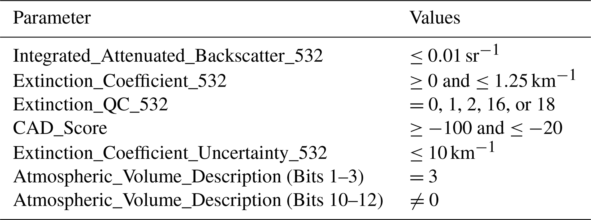
CALIOP, flying aboard the CALIPSO platform within the A-Train satellite constellation, is a dual-wavelength (0.532 and 1.064 µm) lidar that has collected profiles of atmospheric aerosol particles and clouds since summer 2006 (Winker et al., 2007). In this study, daytime and nighttime extinction coefficients retrieved at 0.532 µm from the version 4.10 CALIOP Level 2 5 km aerosol profile (L2_05kmAPro) product were used. Using parameters provided in the L2_05kmAPro product, as well as the corresponding Level 2 5 km aerosol layer (L2_05kmALay) product, a robust quality-assurance (QA) procedure for the aerosol observations was implemented (Table 1). Further information on the QA metrics and screening protocol are discussed in detail in previous studies (Kittaka et al., 2011; Campbell et al., 2012; Toth et al., 2013, 2016). Once the QA procedure was applied, the aerosol profiles were linearly re-gridded from 60 m vertical resolution (above mean sea level, a.m.s.l.) to 100 m segments (i.e., resampled to 100 m resolution) referenced to the local surface (above ground level, a.g.l.; Toth et al., 2014, 2016). The choice of 100 m was arbitrary, and the profiles were re-gridded in order to obtain a dataset corrected for a.g.l., as opposed to the a.m.s.l.-referenced profiles provided by the L2_05kmAPro product. Surface elevation and relative humidity (RH) were taken from collocated model data included in the CALIPSO L2_05kmAPro product (Vaughan et al., 2018; RH was taken from the Modern Era Retrospective-Analysis for Research, or MERRA-2 reanalysis product). To limit the effects of signal attenuation and increase the chances of measuring aerosol presence near the surface, the atmospheric volume description parameter within the L2_05kmAPro dataset is used to cloud-screen each aerosol profile as in Toth et al. (2018).

Table 1 The parameters, and corresponding values, used to assure the quality of the CALIOP aerosol extinction profile.

In this study, near-surface PM mass concentration (C_m) is derived from near-surface CALIOP extinction based on a bulk formulation as in Eq. (1) (e.g., Liou, 2002; Chow et al., 2006):

$$\begin{array}{}\text{(1)}& \mathit{\beta }=C_{\mathrm{m}}\left(a_{\mathrm{scat}}{f}_{\mathrm{rh}}+a_{\mathrm{abs}}\right)\times \mathrm{1000},\end{array}$$

where β is CALIOP-derived near-surface extinction per kilometer, C_m is the PM mass concentration in micrograms per cubic meter, a_scat and a_abs are dry mass scattering and absorption efficiencies in square meters per gram, and f_rh represents the light scattering hygroscopicity. As a preliminary study, for the purpose of demonstrating this concept, we assume the dominant aerosol type over the CONUS is pollution aerosol (i.e., the most prevalent near-surface aerosol type reported in the CALIOP products for the CONUS during 2008–2009 is polluted continental) with a_scat and a_abs values of 3.40 and 0.37 m² g⁻¹ (Hess et al., 1998; Lynch et al., 2016), respectively. These values are similar to those reported in Hand and Malm (2007) and Kaku et al. (2018) but are interpolated to 0.532 µm from values at 0.450 and 0.550 µm obtained from the Optical Properties of Aerosols and Clouds (OPAC) model (Hess et al., 1998). Still, both a_scat and a_abs have regional and species-related dependencies. Also, only 2-year averages are used in this study, and we assume that sporadic aerosol plumes are smoothed out in the averaging process and that bulk aerosol properties are similar throughout the study region. We have further explored the impact of aerosol types on PM_2.5 retrievals in a later section. Furthermore, to aid in focusing this study on fine-mode and anthropogenic aerosols, those aerosol extinction range bins classified as dust by the CALIOP typing algorithm were excluded from the analysis.

Also, surface PM concentrations are dry mass measurements. To account for the impact of humidity on a_scat (it is assumed that a_abs is not affected by moisture; Nessler et al., 2005; Lynch et al., 2016), we estimated the hygroscopic growth factor for pollution aerosol based on Hänel (1976), as shown in Eq. (2):

$$\begin{array}{}\text{(2)}& f_{\mathrm{rh}}={\left({\displaystyle \frac{\mathrm{1}-\text{RH}}{\mathrm{1}-{\text{RH}}_{\mathrm{ref}}}}\right)}^{-\mathrm{\Gamma }},\end{array}$$

where f_rh is the hygroscopic growth factor, RH is the relative humidity, and RH_ref is the reference RH and is set to 30 % in this study (Lynch et al., 2016). Γ is a unitless value (a fit parameter describing the amount of hygroscopic increase in scattering) and is assumed to be 0.63 (i.e., sulfate aerosol) in this study (Hänel, 1976; Chew et al., 2016; Lynch et al., 2016).

Additionally, the CALIOP-derived PM density is for all particle sizes. To convert from mass concentration of PM (C_m) to mass concentration of PM_2.5 (C_m2.5), which represents mass concentration for particle diameters smaller than 2.5 µm, we adopted the PM_2.5-to-PM₁₀ (PM with diameters less than 10 µm) ratio (φ) of 0.6 as measured during the Studies of Emissions and Atmospheric Composition, Clouds and Climate Coupling by Regional Surveys (SEAC4RS) campaign over the US (Kaku et al., 2018). Again, the ratio of PM_2.5 to PM₁₀ can also vary spatially; however we used a regional mean to demonstrate the concept. Analyses in a later section using 2 years (2008–2009) of surface PM_2.5 to PM₁₀ data suggest that 0.6 is a rather reasonable number to use for the CONUS for the study period. Here we assume that mass concentrations for particle diameters larger than 10 µm are negligible over the CONUS. Thus, we can rewrite Eq. (1) as

$$\begin{array}{}\text{(3)}& C_{\mathrm{m}\mathrm{2.5}}={\displaystyle \frac{\mathit{\beta }\times \mathit{\varphi }}{\left(a_{\mathrm{scat}}\times f_{\mathrm{rh}}+a_{\mathrm{abs}}\right)\times \mathrm{1000}}},\end{array}$$

where C_m2.5 is the CALIOP-derived PM_2.5 concentration in units of micrograms per cubic meter.

Lastly, we note that most of the results are shown in the form of scatter plots with fits from a Deming regression (Deming, 1943). Due to uncertainties in PM_2.5 data, we show slopes computed from Deming regression analyses instead of those from simple linear regression. Deming regression in particular is appropriate here, as it accounts for errors in both the independent and dependent variables (Deming, 1943) and has been used in past PM_2.5-related studies (e.g., Huang et al., 2014).

3 Results and discussion

3.1 Regional analysis

Figure 2a shows the mean PM_2.5 concentration using 2 years (2008–2009) of daily surface PM_2.5 data from the U.S. EPA (PM_{2.5_EPA}), not collocated with CALIOP observations. A total of 1091 stations (some operational throughout the entire period; others only partially) are included in the analysis, and observations from those stations are further used in evaluating CALIOP-derived PM_2.5 concentrations (C_m2.5), as later shown in Fig. 3. PM_2.5 concentrations of ∼10 µg m⁻³ are found over the eastern CONUS. In comparison, much lower PM_2.5 concentrations of ∼5 µg m⁻³ are exhibited for the interior CONUS, over states including Montana, Wyoming, North Dakota, South Dakota, Utah, Colorado, and Arizona. For the west coast of the CONUS, and especially over California, higher PM_2.5 concentrations are observed, with the maximum 2-year mean near 20 µg m⁻³. Note that the spatial distribution of surface PM_2.5 concentrations over the CONUS as shown in Fig. 2a is consistent with reported values from several studies (e.g., Hand et al., 2013; Van Donkelaar et al., 2015; Di et al., 2017).

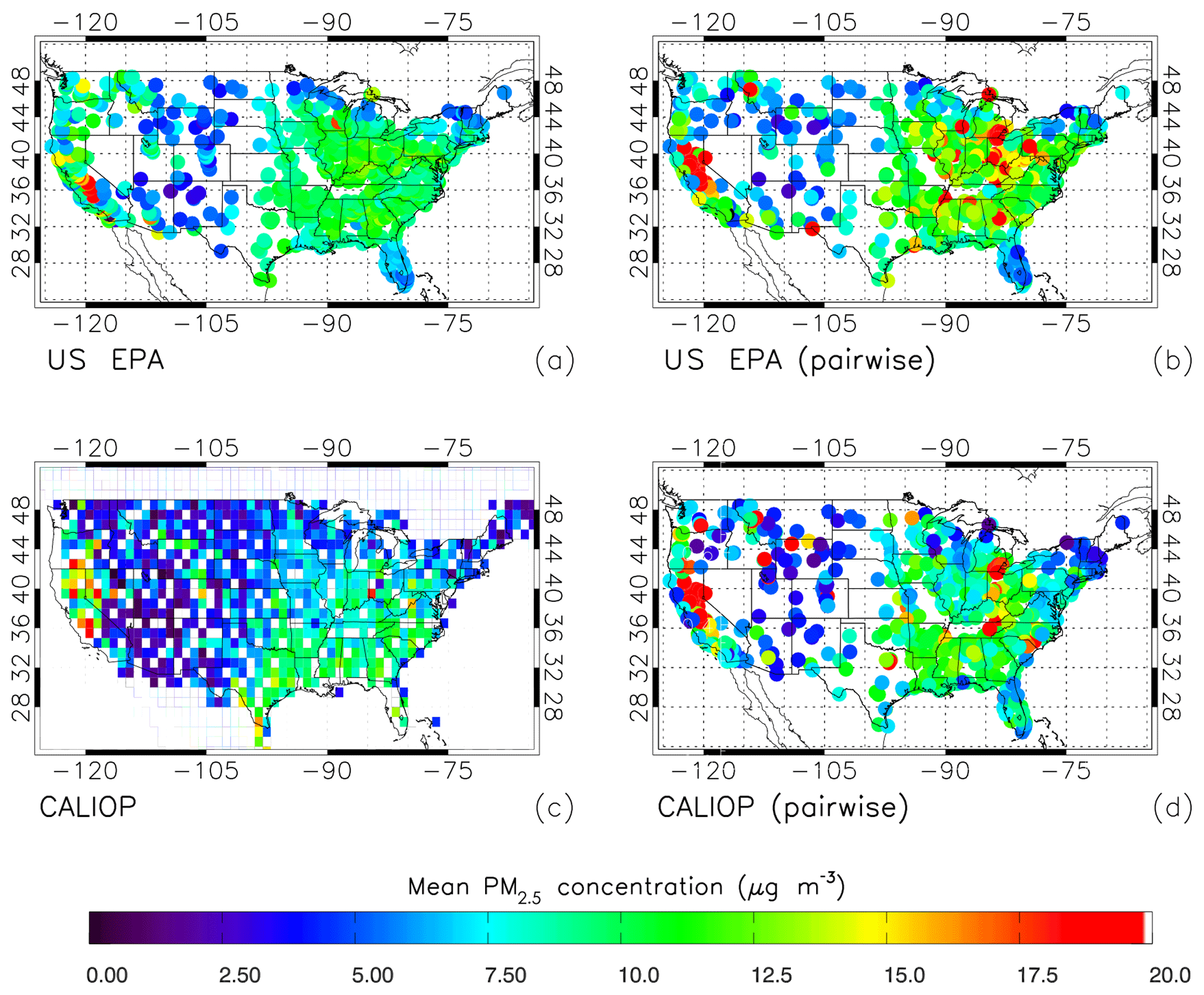
Figure 2 For 2008–2009 over the CONUS, (a) mean PM_2.5 concentration (µg m⁻³) for those U.S. EPA stations with reported daily measurements, and (c) 1^∘ × 1^∘ average CALIOP-derived PM_2.5 concentrations for the 100–1000 m a.g.l. atmospheric layer, using Eq. (3), for combined daytime and nighttime conditions. Also shown are the pairwise PM_2.5 concentrations from (b) EPA daily measurements and (d) those derived from CALIOP (day and night combined), both averaged for each EPA station for the 2008–2009 period. For all four plots, values greater than 20 µg m⁻³ are colored red.

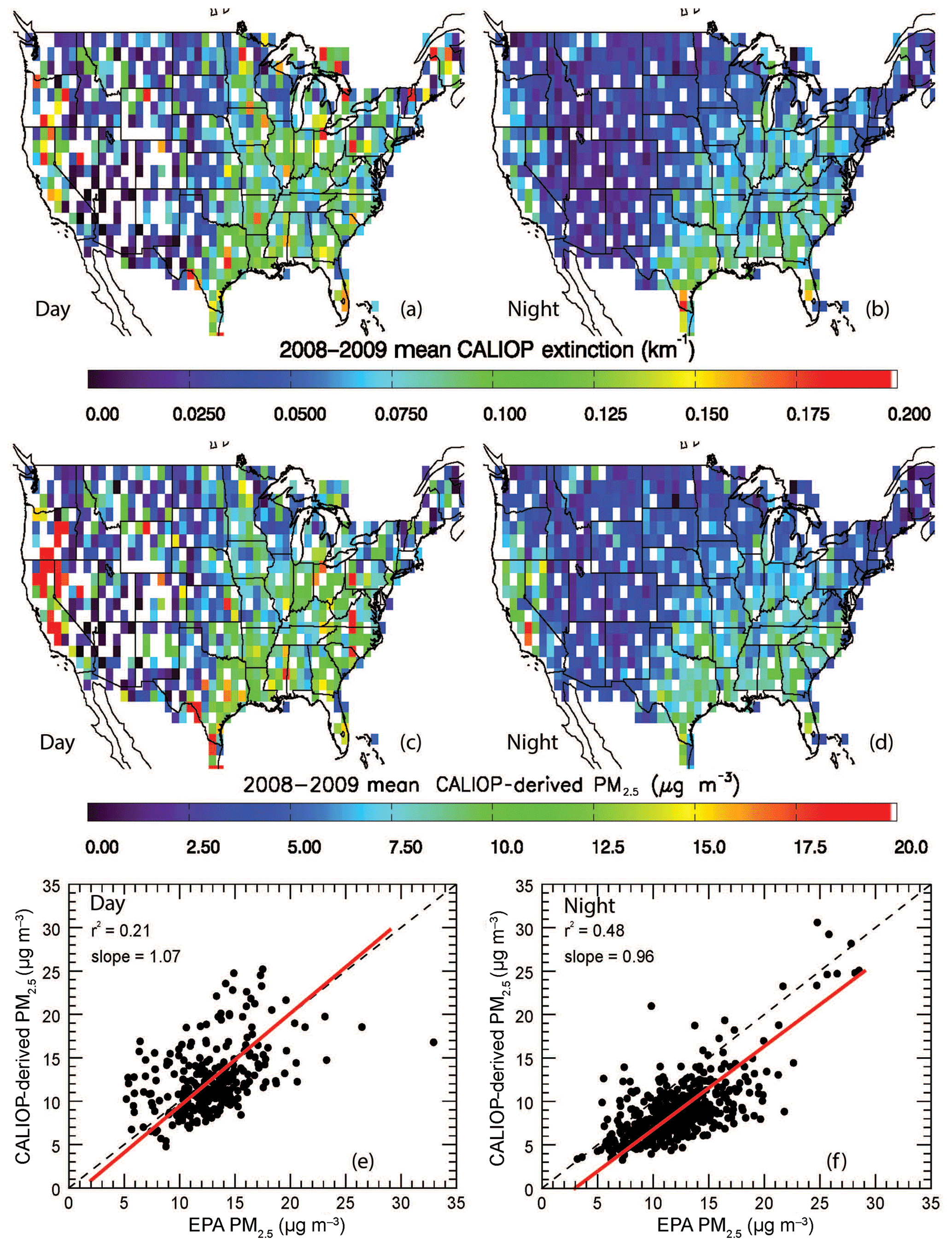
Figure 3 For 2008–2009 over the CONUS, 1^∘ × 1^∘ average CALIOP extinction, relative to the number of cloud-free 5 km CALIOP profiles in each 1^∘ × 1^∘ bin, for the 100–1000 m a.g.l. atmospheric layer, for (a) daytime and (b) nighttime measurements. Also shown are the corresponding CALIOP-derived PM_2.5 concentrations, using Eq. (3) for (c) daytime and (d) nighttime conditions. Values greater than 0.2 km⁻¹ and 20 µg m⁻³ for (a, b) and (c, d), respectively, are colored red. Scatter plots of mean PM_2.5 concentration from ground-based U.S. EPA stations and those derived from collocated near-surface CALIOP observations are shown in the bottom row, using (e) daytime and (f) nighttime CALIOP data. The red lines represent the Deming regression fits.

Figure 3a shows the 2-year averaged 1^∘ × 1^∘ (latitude and longitude) gridded daytime CALIOP aerosol extinction over the CONUS using CALIOP observations from 100 to 1000 m, referenced to the number of cloud-free L2_05kmAPro profiles in each 1×1^∘ bin. The lowest 100 m of CALIOP extinction data are not used in the analysis due to the potential of surface return contamination (e.g., Toth et al., 2014), although this has been improved for the version 4 CALIOP products but may still be present in some cases. Here the averaged extinction from 100–1000 m is used to represent near-surface aerosol extinction. This selection of the 100–1000 m layer is somewhat arbitrary, even though it is estimated from the mean CALIOP-based aerosol vertical distribution over the CONUS (Toth et al., 2014). Thus, a sensitivity study is provided in a later section to understand the impact of this aerosol layer selection on CALIOP-based PM_2.5 retrievals. As shown in Fig. 3a, a higher mean near-surface CALIOP extinction of 0.1 km⁻¹ is found for the eastern CONUS and over California, while lower values of 0.025–0.05 km⁻¹ are found for the interior CONUS. Figure 3b shows a plot similar to Fig. 3a but using nighttime CALIOP observations only. Although similar spatial patterns are found during both day and night, the near-surface extinction values are overall lower for nighttime than daytime, and nighttime data are less noisy than daytime. These findings are not surprising, as daytime CALIOP measurements are subject to contamination from background solar radiation (e.g., Omar et al., 2013).

To investigate any diurnal biases in the data, Fig. 3c and d show the derived PM_2.5 concentration using daytime and nighttime CALIOP data, respectively, based on the method described in Sect. 2. Both Fig. 3c and d suggest a higher PM_2.5 concentration of ∼10–12.5 µg m⁻³ over the eastern CONUS and a much lower PM_2.5 concentration of ∼2.5–5 µg m⁻³ over the interior CONUS. High PM_2.5 values of 10–20 µg m⁻³ are also found over the west coast of the CONUS, particularly over California. The spatial distribution of PM_2.5 concentrations, as derived using near-surface CALIOP data (Fig. 3c and d, as well as the combined daytime and nighttime perspective shown in Fig. 2c), is remarkably similar to the spatial distribution of PM_2.5 values as estimated based on ground-based observations (Fig. 2a). Still, day and night differences in PM_2.5 concentrations are also clearly visible, as higher PM_2.5 values are found, in general, during daytime, based on CALIOP observations. The high daytime PM_2.5 values, as shown in Fig. 3c, may represent stronger near-surface convection and more frequent anthropogenic activities during daytime. However, they may also be partially contributed by solar radiation contamination. Another possibility is that the daytime mean extinction coefficients (from which the mean PM_2.5 estimates are derived) appear artificially larger than at night due to high daytime noise limiting the ability of CALIOP to detect fainter aerosol layers during daylight operations. Note that, for context, maps of the number of days and CALIOP Level 2 5 km aerosol profiles used in the creation of Fig. 3a–d are shown in Appendix Fig. A1.

Figure 3e shows the intercomparison between PM_{2.5_EPA} and PM_{2.5_CALIOP} concentrations. Note that only CALIOP and ground-based PM_2.5 data pairs, which are within 100 km of each other and have reported values for the same day (i.e., year, month, and day), are used to generate Fig. 3e. Still, although only spatially and temporally collocated data pairs are used, ground-based PM_2.5 data represent 24 h averages, while CALIOP-derived PM_2.5 concentrations are instantaneous values over the daytime CALIOP overpass. To reduce this temporal bias, 2 years (2008–2009) of collocated CALIOP-derived and measured PM_2.5 concentrations are averaged and only the 2-year averages are used in constructing Fig. 3e. Also, to minimize the abovementioned temporal sampling bias, ground stations with fewer than 100 collocated pairs are discarded. This leaves a total of 276 stations for constructing Fig. 3e.

As shown in Fig. 3e, an r² value of 0.21 (with slope of 1.07) is found between CALIOP-derived and measured surface PM_2.5 concentrations, with a corresponding mean bias of −0.40 µg m⁻³ (PM_{2.5_CALIOP}−PM_{2.5_EPA}). In comparison, Fig. 3f shows results similar to Fig. 3e, but for nighttime CALIOP data. A much higher r² value of 0.48 (with slope of 0.96) is found between CALIOP-derived and measured PM_2.5 values from 528 EPA stations, with a corresponding mean bias of −3.3 µg m⁻³ (PM_{2.5_CALIOP}−PM_{2.5_EPA}). This may be related to the diurnal variability of PM_2.5 concentrations, as the daily mean EPA measurement might be closer to the CALIOP morning retrieval than to its afternoon counterpart. Still, data points are more scattered in Fig. 3e in comparison with Fig. 3f, which again indicates that daytime CALIOP data are noisier, possibly due to daytime solar contamination as well as other factors such as biases in relative humidity. Details of these biases are further explored in Sect. 3.2.

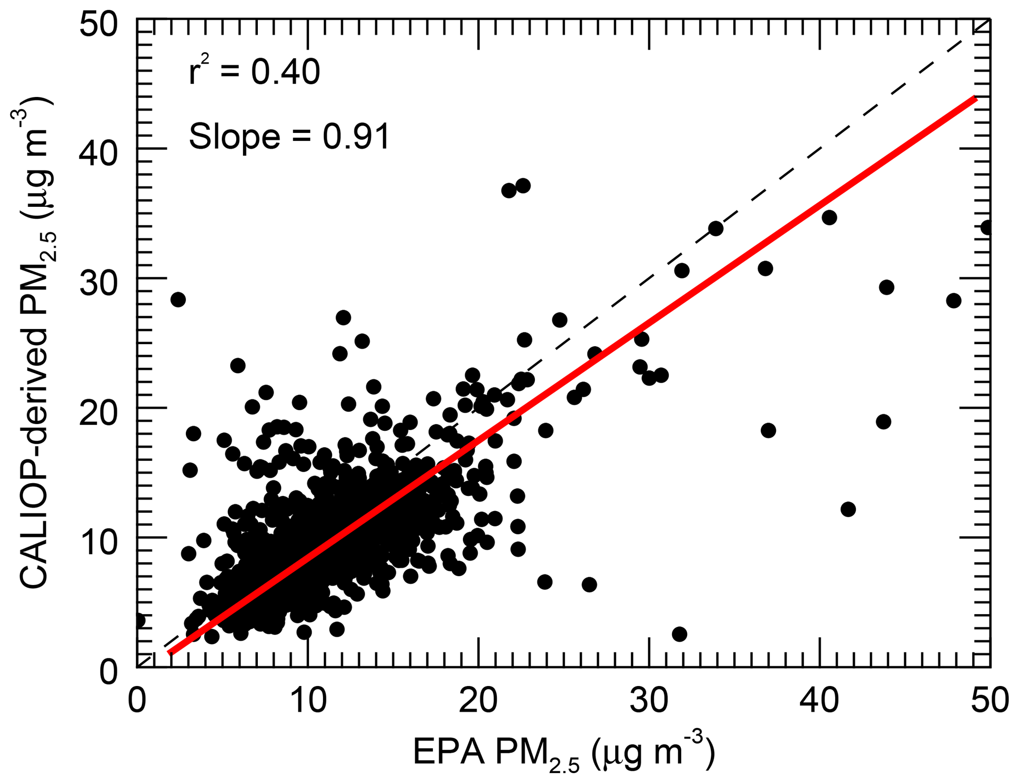
Figure 4 Scatter plot of mean PM_2.5 concentration from ground-based U.S. EPA stations and those derived from collocated near-surface CALIOP observations using combined daytime and nighttime CALIOP data. The red line represents the Deming regression fit.

To supplement this analysis, a pairwise PM_{2.5_EPA} and PM_{2.5_CALIOP} (day and night CALIOP combined) analysis is presented in the spatial plots of Fig. 2b and d. Here, however, we lift the requirement of 100 collocated pairs to increase data samples for better spatial representativeness. The spatial variability of PM_2.5 over the CONUS is consistent with the observed patterns of non-collocated data (i.e., Fig. 2a and c), but with generally higher values due to differences in sampling. Also, comparing Fig. 2b and d, PM_{2.5_EPA} spatial patterns match well with those of PM_{2.5_CALIOP}, yet with larger values for PM_{2.5_EPA} (consistent with the biases discussed above). Lastly, a scatter plot of the pairwise analysis shown in Fig. 2b and d is provided in Fig. 4. An r² value of 0.40 is found between EPA and CALIOP-derived PM_2.5 concentrations from a combined daytime and nighttime CALIOP perspective. Overall, Figs. 2, 3, and 4 indicate that near-surface CALIOP extinction data can be used to estimate surface PM_2.5 concentrations with reasonable accuracy.

3.2 Uncertainty analysis

In this section, uncertainties in the CALIOP-derived 2-year averaged PM_2.5 concentrations are explored as functions of aerosol vertical distribution, PM_2.5-to-PM₁₀ ratio, RH, aerosol type, and cloud presence above. Spatial-sampling-related biases as well as prognostic errors are also studied.

3.2.1 Prognostic errors in C_m2.5

As a first step for the uncertainty analysis, we estimated the prognostic error of 2-year averaged PM_{2.5_CALIOP}. Figure 5 shows the root-mean-square error (RMSE) of CALIOP-based PM_2.5 concentrations against those from EPA stations as a function of CALIOP-based PM_2.5 for the 2008–2009 period over the CONUS. RMSEs were computed for five equally sampled bins, determined from a cumulative histogram analysis. Each point in Fig. 5, from left to right, represents the RMSE and mean PM_2.5 concentration derived from CALIOP for 0 %–20 %, 20 %–40 %, 40 %–60 %, 60 %–80 %, and 80 %–100 % cumulative frequencies. A mean combined daytime and nighttime RMSE of ∼4 µg m⁻³ is found, with a mean value slightly greater for nighttime (∼ 4.3 µg m⁻³) than daytime (∼3.7 µg m⁻³). While most bins exhibit larger nighttime RMSEs, daytime RMSEs are larger for the greatest mean CALIOP-derived PM_2.5 concentrations.

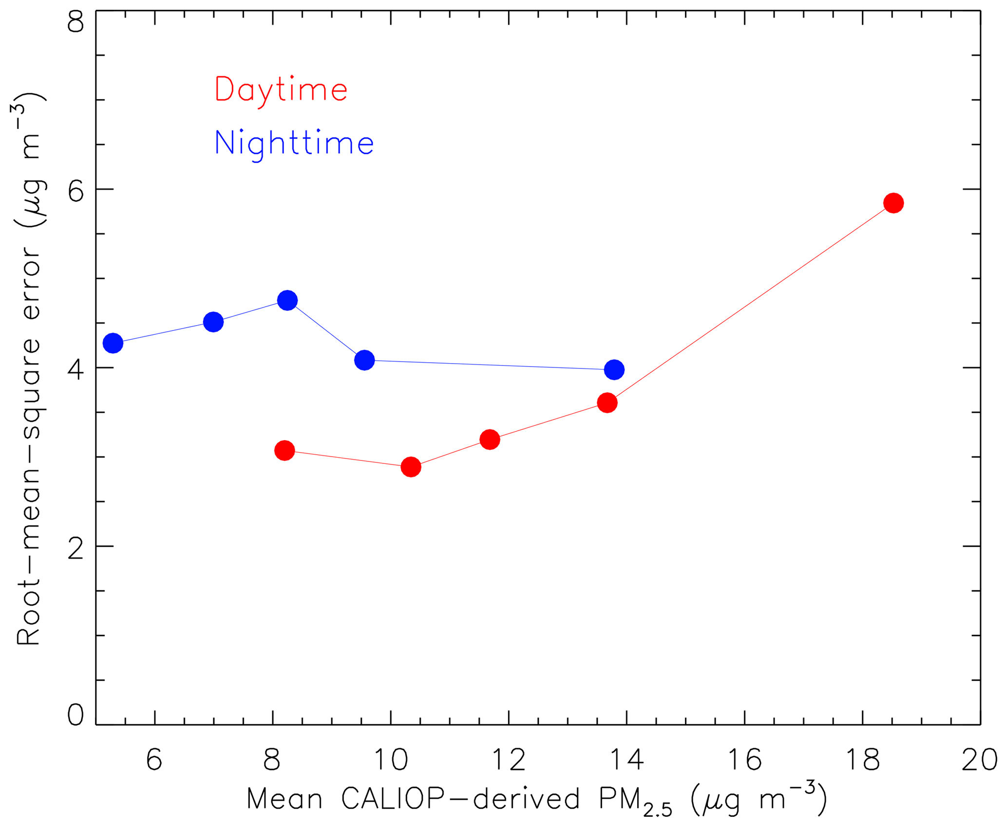
Figure 5 Root-mean-square errors of CALIOP-derived PM_2.5 against EPA PM_2.5 as a function of CALIOP-derived PM_2.5, using both daytime (in red) and nighttime (in blue) CALIOP observations. The five bins are equally sampled based upon a cumulative histogram analysis, and each point from left to right represents the RMSE and mean PM_2.5 concentration derived from CALIOP for 0 %–20 %, 20 %–40 %, 40 %–60 %, 60 %–80 %, and 80 %–100 % cumulative frequencies.

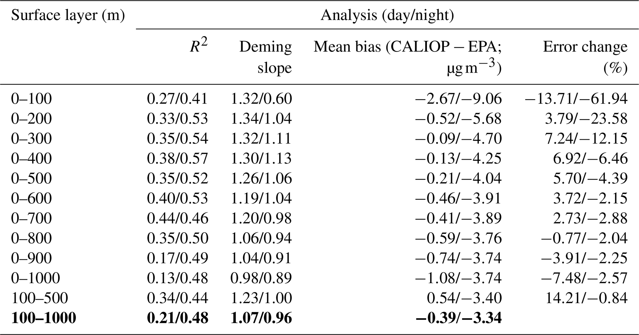
Table 2 Statistical summary of a sensitivity analysis varying the height of the surface layer, including R², slope from Deming regression, mean bias (CALIOP−EPA) of PM_2.5 in micrograms per cubic meter, and percent error change in derived PM_2.5, defined as $\left(\right({\text{mean new PM}}_{\mathrm{2.5}}-{\text{mean original PM}}_{\mathrm{2.5}})/{\text{mean original PM}}_{\mathrm{2.5}})\times \mathrm{100}$. The row in bold represents the results shown in the remainder of the paper.

3.2.2 Surface layer height sensitivity study

A sensitivity study was conducted for which PM_2.5 was derived from near-surface CALIOP aerosol extinction by varying the height of the surface layer in increments of 100 m from the ground to 1000 m. Note that the surface layer (0–100 m) is included for this sensitivity study only. The statistical results of this analysis, for both daytime and nighttime conditions, are shown in Table 2. Four statistical parameters were computed, consisting of r², slope from Deming regression, mean bias (CALIOP−EPA) of PM_2.5, and percent error change in derived PM_2.5, defined as $\left(\right(\mathrm{mean}\mathrm{\_}\mathrm{new}\mathrm{\_}{\mathrm{PM}}_{\mathrm{2.5}}-\mathrm{mean}\mathrm{\_}\mathrm{original}\mathrm{\_}{\mathrm{PM}}_{\mathrm{2.5}})/\mathrm{mean}\mathrm{\_}\mathrm{original}\mathrm{\_}{\mathrm{PM}}_{\mathrm{2.5}})\times \mathrm{100}$. For context, the bottom row of Table 2 shows the results from the original analysis. In terms of r² and slope, optimal values peak at different surface layer heights between daytime and nighttime. For example, for daytime, the largest correlations are found for the 0–600 and 0–700 m layers, while for nighttime these are found for the 0–300 and 0–400 m layers. However, the 0–300 m layer exhibits the lowest mean bias for the daytime analysis, and the 100–1000 m layer exhibits the lowest mean bias for the nighttime analysis. Overall, marginal changes are found for varying the height of the surface layer. Yet the largest mean bias is found for the 0–100 m layer, indicating the need for excluding the 0–100 m layer in the analysis.

3.2.3 RH sensitivity study

Profiles of RH were taken from the MERRA-2 reanalysis product, as these collocated data are provided in the CALIPSO L2_05kmAPro product. However, biases may exist in this RH dataset. Thus, we examined the impact of varying the RH values by ±10 % on the CALIOP-derived PM_2.5 concentrations. For both daytime and nighttime analyses, no significant differences in the r² and slope values were found. However, a +15 % change in the mean derived PM_2.5 values was found by decreasing the RH values by 10 %, while a −15 % change in the mean derived PM_2.5 values was found by increasing the RH values by 10 %.

3.2.4 PM_2.5-to-PM₁₀ ratio sensitivity study

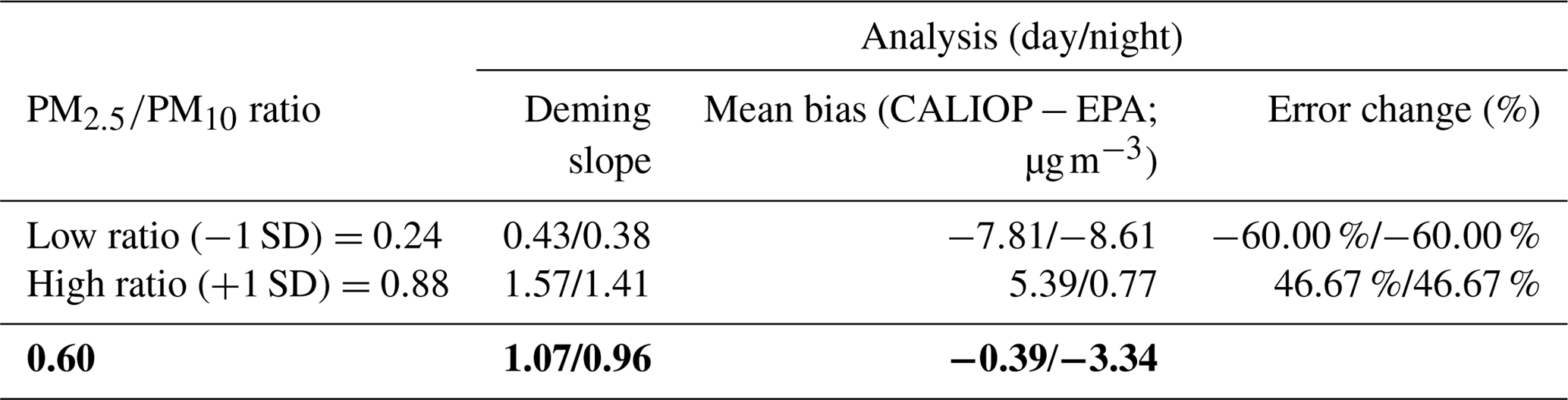
Another source of uncertainty in this study is the PM_2.5∕PM₁₀ ratio. Using surface-based PM_2.5 and PM₁₀ data from those EPA stations over the CONUS for 2008–2009 with concurrent PM_2.5 and PM₁₀ daily data available (i.e., 409 stations), we computed the mean PM_2.5∕PM₁₀ ratio and its corresponding standard deviation. The mean ratio was 0.56 with a standard deviation of 0.32. It is interesting to note that the mean PM_2.5∕PM₁₀ ratio estimated from 2 years of surface observations over the CONUS is close to 0.6 (the number used in this study), as reported by Kaku et al. (2018). We also tested the sensitivity of the derived PM_2.5 concentrations as a function of PM_2.5∕PM₁₀ ratio for two scenarios: ±1 standard deviation of the mean (Table 3). In general, a ±50 % to 60 % change is found with the variation in the PM_2.5∕PM₁₀ ratio at the range of ±1 standard deviation of the mean. As suggested from Table 3, the lowest mean daytime bias is found for a ratio of 0.6, and for nighttime the lowest mean bias occurs using a ratio of 0.88.

Table 3 Statistical summary of a sensitivity analysis varying the PM_2.5-to-PM₁₀ ratio used, including slope from Deming regression, mean bias (CALIOP−EPA) of PM_2.5 in micrograms per cubic meter, and percent error change in derived PM_2.5, defined as $\left(\right({\text{mean new PM}}_{\mathrm{2.5}}-{\text{mean original PM}}_{\mathrm{2.5}})/{\text{mean original PM}}_{\mathrm{2.5}})\times \mathrm{100}$. The row in bold represents the results shown in the remainder of the paper.

3.2.5 Sampling-related biases

As mentioned in the introduction section, a sampling bias, due to the very small footprint size and ∼16-day repeat cycle of CALIOP, can exist when using CALIOP observations for PM_2.5 estimates (Zhang and Reid, 2009). This sampling-induced bias is investigated from a 2-year mean perspective by comparing histograms of PM_{2.5_EPA} and C_m2.5 concentrations as shown in Fig. 6. To generate Fig. 6, all available daily EPA PM_2.5 data are used to represent the “true” 2-year mean spectrum of PM_2.5 concentrations over the EPA sites. The aerosol extinction data spatially collocated to the EPA sites (Sect. 3.1), but not temporally collocated, are used for estimating the 2-year mean spectrum of PM_2.5 concentrations as derived from CALIOP observations. To be consistent with the previous analysis, only cloud-free CALIOP profiles are considered. The PM_{2.5_EPA} concentrations peak at ∼10 µg m⁻³ (standard deviation of ∼3 µg m⁻³), and CALIOP-derived PM_2.5 peaks at ∼9 µg m⁻³ (daytime; standard deviation of ∼4 µg m⁻³) and ∼7 µg m⁻³ (nighttime; standard deviation of ∼2 µg m⁻³). The distribution shifts towards smaller concentrations for CALIOP, more so for nighttime than daytime (possibly due to CALIOP daytime versus nighttime detection differences).

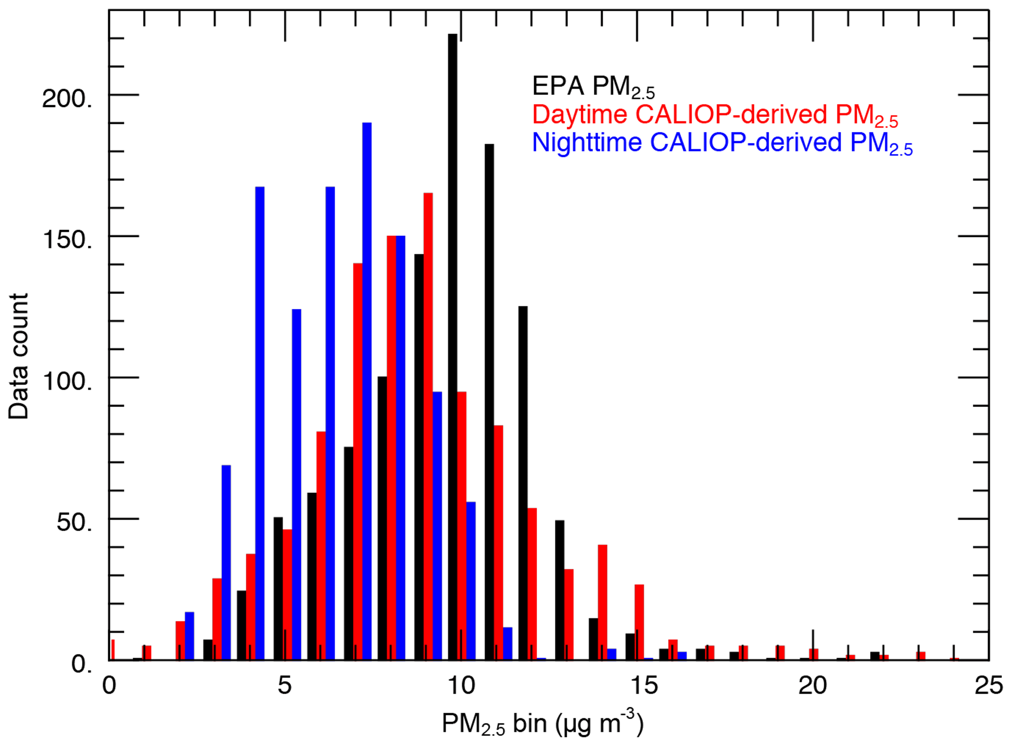
Figure 6 The 2-year (2008–2009) histograms of mean PM_2.5 concentrations from the U.S. EPA (in black) and those derived from aerosol extinction using nighttime (in blue) and daytime (in red) CALIOP data. The U.S. EPA data shown are not collocated, while those derived using CALIOP are spatially (but not temporally) collocated, with EPA station observations.

Still, Fig. 6 may reflect the diurnal difference in PM_2.5 concentrations as well as the retrieval bias in C_m2.5 values. Thus, we have re-performed the exercise shown in Fig. 6 using spatially and temporally collocated PM_{2.5_EPA} and C_m2.5 data as shown in Fig. 7. To construct Fig. 7, PM_{2.5_EPA} and C_m2.5 data are collocated following the steps mentioned in Sect. 3.1, with CALIOP and EPA PM_2.5 representing 2-year mean values for each EPA station. Again, only cloud-free CALIOP profiles are considered for this analysis. As shown in Fig. 7a, the PM_{2.5_EPA} concentrations peak at ∼12 µg m⁻³ (standard deviation of ∼4 µg m⁻³), and daytime C_m2.5 peaks at ∼10 µg m⁻³ (standard deviation of ∼4 µg m⁻³). In comparison, with the use of collocated nighttime C_m2.5 and PM_{2.5_EPA} data as shown in Fig. 7b, the peak PM_{2.5_EPA} value is about 5 µg m⁻³ higher than the peak C_m2.5 value (with similar standard deviations as found in the analyses of Fig. 7a). Considering both Figs. 6 and 7, it is likely that the temporal sampling bias seen in Fig. 6 is at least in part due to retrieval bias as well as the difference in PM_2.5 concentrations during daytime and nighttime.

Figure 7 The 2-year (2008–2009) histograms of mean PM_2.5 concentrations from the U.S. EPA and those derived from spatially and temporally collocated aerosol extinction using (a) daytime and (b) nighttime CALIOP data.

3.2.6 CALIOP AOD analysis

Most past studies focused on the use of column AODs as proxies for surface PM_2.5 (e.g., Liu et al., 2005; Hoff and Christopher, 2009; van Donkelaar et al., 2015). Therefore, it is interesting to investigate whether near-surface CALIOP extinction values can be used as a better physical quantity to estimate surface PM_2.5 in comparing with column-integrated CALIOP AOD. To achieve this goal, we have compared CALIOP column AOD and PM_2.5 from EPA stations, as shown in Fig. 8. Similar to the scatter plots of Fig. 3, each point represents a 2-year mean for each EPA site and was created from a dataset following the same spatial–temporal collocation as described above. As shown in Fig. 8, r² values of 0.04 and 0.13 are found using CALIOP daytime and nighttime AOD data, respectively, similar to the MODIS-based analysis shown in Fig. 1. This is expected, as elevated aerosol layers will negatively impact the relationship between surface PM_2.5 and column AOD. The derivation of surface PM_2.5 from near-surface CALIOP extinction, as demonstrated from this study, however, provides a much better spatial matching between the quantities being compared, with potential error terms that can be well quantified and minimized in later studies.

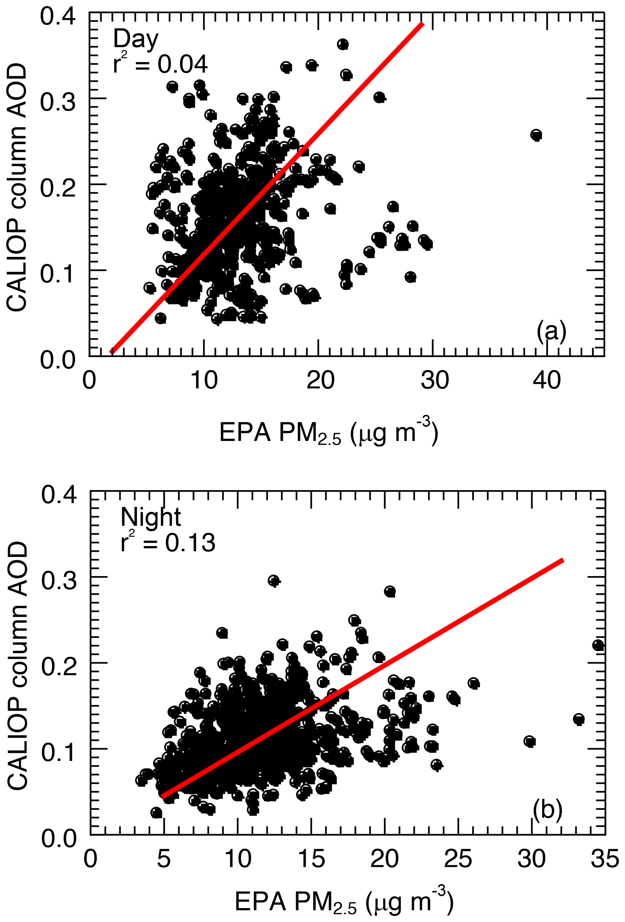
Figure 8 For 2008–2009, scatter plots of mean PM_2.5 concentration from ground-based U.S. EPA stations and mean column AOD from collocated CALIOP observations, using (a) daytime and (b) nighttime CALIOP data. The red lines represent the Deming regression fits.

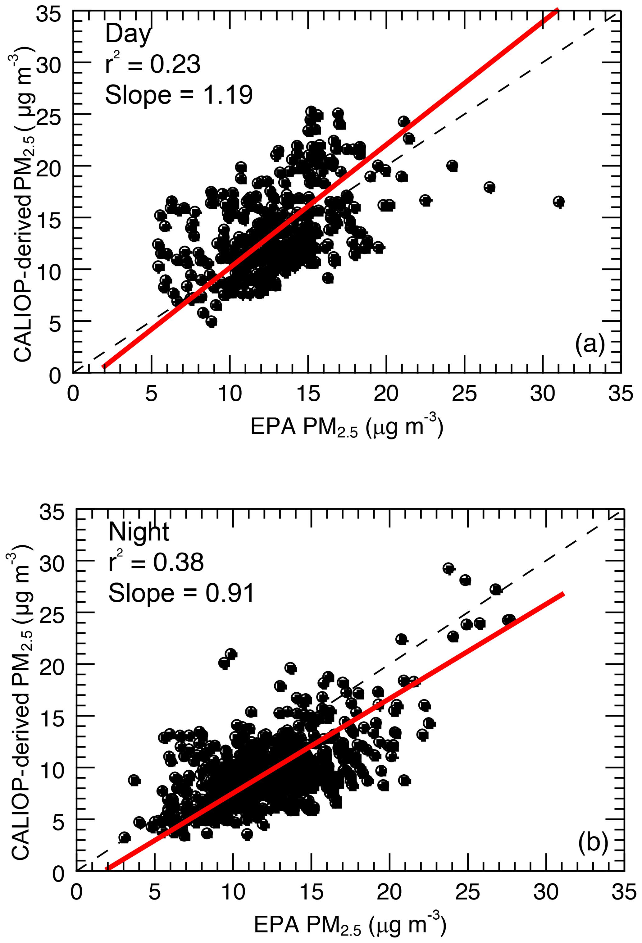
Figure 9 For 2008–2009, scatter plots of mean PM_2.5 concentration from ground-based U.S. EPA stations and those derived from collocated all-sky (including cloud-free and cloudy profiles) near-surface CALIOP observations, using (a) daytime and (b) nighttime CALIOP data. The red lines represent the Deming regression fits.

3.2.7 Cloud flag sensitivity study

For most of this paper, a strict cloud screening process is implemented, during which no clouds are allowed in the entire CALIOP profile. However, in contrast to passive sensor capabilities (e.g., MODIS), near-surface aerosol extinction coefficients can be readily retrieved from CALIOP profiles even when there are transparent cloud layers above. Therefore, we conducted an additional analysis for which no cloud flag was set (i.e., all-sky conditions). Results are shown in scatter plot form in Fig. 9, in a manner similar to in Fig. 3e and f, with an additional 97 points for the daytime analysis and 156 points for the nighttime analysis. Comparing the all-sky results with those of Fig. 3e and f (cloud-free conditions), the r² values are similar. This is also true in terms of mean bias, with similar values of 0.70 µg m⁻³ found for daytime, and −2.68 µg m⁻³ for nighttime, all-sky scenarios. This indicates that our method performs reasonably well from an all-sky perspective. However, we note that restricting the analysis to solely those cases that are cloudy (not shown), the method does not perform as well. For example, the r² value decreases by 71 % for the daytime analysis compared to the cloud-free results (Fig. 3e). The corresponding nighttime r² value decreases by 90 %. This is expected, as any errors made in estimating the optical depths of the overlying clouds will propagate (as biases) into the extinction retrievals for the underlying aerosols.

3.2.8 Aerosol type analysis

Also, for this study, we assume that the primary aerosol type over the CONUS is pollution (i.e., sulfate) aerosol, which is generally composed of smaller (fine mode) particles that tend to exhibit mass extinction efficiencies ∼4 m² g⁻¹. However, even after implementing our dust-free restriction, the study region can also be contaminated with non-pollution aerosols, which can have a larger particle size and exhibit lower mass extinction efficiencies (e.g., Hess et al., 1998; Malm and Hand, 2007; Lynch et al., 2016). The use of PM_2.5 versus PM₁₀ somewhat mitigates this size dependency, but nevertheless coarse mode dust or sea salt can dominate PM_2.5 mass values (e.g., Atwood et al., 2013).

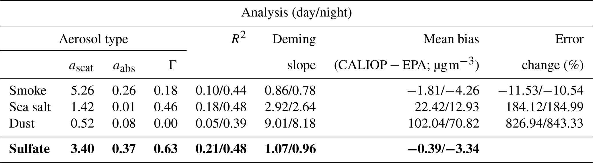
Thus, in this section, the impact of aerosol types on the derived PM_2.5 concentrations was explored by varying the mass scattering and absorption efficiencies and gamma values associated with each aerosol type. The three aerosol types chosen for this sensitivity study were dust, sea salt, and smoke, based upon Lynch et al. (2016). The mass scattering and absorption values for dust and sea salt were interpolated to 0.532 µm from values at 0.450 and 0.550 µm from OPAC (as was performed for the sulfate case; Hess et al., 1998). For smoke, these values were interpolated to 0.532 µm from values at 0.440 and 0.670 µm as provided by Reid et al. (2005) for smoke cases over the US and Canada. The gamma values were taken from Lynch et al. (2016) and the references within. These values, as well as the results from this sensitivity study, are shown in Table 4. If we assume all aerosols within the study region are smoke aerosols, no major changes in the retrieved CALIOP PM_2.5 values are found. However, significant uncertainties on the order of ∼200 % are found if sea salt, or ∼800 % if dust, aerosol mass scattering and absorption efficiencies and gamma values are used instead. Clearly, this study suggests that accurate aerosol typing is necessary for future applications of CALIOP observations for surface PM_2.5 estimations.

Table 4 Statistical summary of a sensitivity analysis varying the aerosol type assumed in the derivation of PM_2.5, including R², slope from Deming regression, mean bias (CALIOP−EPA) of PM_2.5 in micrograms per cubic meter, and percent error change in derived PM_2.5, defined as $\left(\right({\text{mean new PM}}_{\mathrm{2.5}}-{\text{mean original PM}}_{\mathrm{2.5}})/{\text{mean original PM}}_{\mathrm{2.5}})\times \mathrm{100}$. The row in bold represents the results shown in the remainder of the paper.

3.3 E-folding correlation length for PM_2.5 concentrations over the CONUS

As a last study, we also estimated the spatial e-folding correlation length for PM_2.5 concentrations over the CONUS. This provides us an estimation of the correlation between a CALIOP-derived and actual PM_2.5 concentration for a given location as a function of distance between the CALIOP observation and the given location. To accomplish this, all EPA stations over the CONUS with at least 50 days of daily data available for the 2008–2009 period were first determined. Next, the distances between each pair of these EPA stations, and their corresponding correlation of daily PM_2.5 concentrations, were computed. Results are shown in Fig. 10 as a scatter plot, with individual points in gray and the black curve representing the exponential fit to the data. A decrease in PM_2.5 correlation with distance between EPA stations is found, and the e-folding length in correlation (e.g., correlation reduced to 1∕e, or 0.37) is ∼600 km (from an AOD standpoint, this value is 40–400 km, as suggested by Anderson et al., 2003).

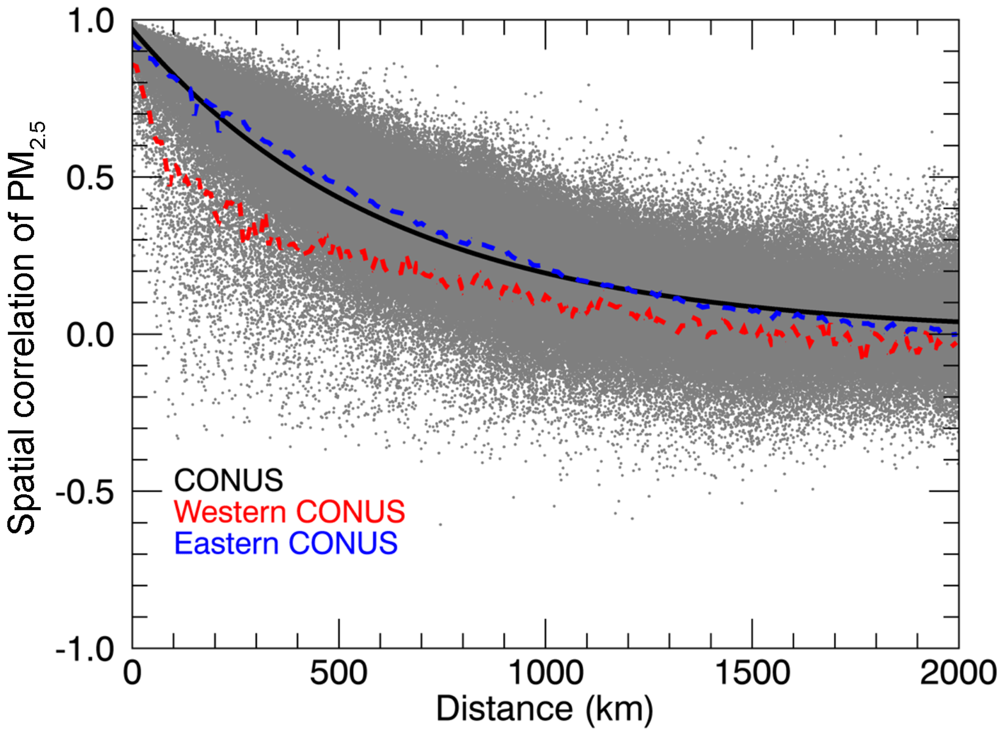
Figure 10 For 2008–2009 over the CONUS, scatter plot of distance (km) between any two U.S. EPA stations and the corresponding spatial correlation of PM_2.5 concentration between each pair of stations. The black curve represents the exponential fit to the data for the entire CONUS, and the red and blue dashed lines represent 10 km bin averages for the western and eastern CONUS, respectively.

Also included in Fig. 10 are results from a corresponding regional analysis, with the red and blue lines showing bin averages (10 km) for the western and eastern CONUS, respectively (regions partitioned by the −97^∘ longitude line). The e-folding length is ∼300 km for the western CONUS and ∼700 km for the eastern CONUS, indicating a much shorter correlation length for pollution over the western CONUS, possibly due to a more complex terrain such as mountains. Overall, these PM_2.5 e-folding lengths suggest that CALIOP-derived PM_2.5 concentrations could still have some representative skill within a few hundred kilometers of a given location.

4 Conclusions

In this paper, we have demonstrated a new bulk-mass-modeling method for retrieving surface particulate matter (PM) with particle diameters smaller than 2.5 µm (PM_2.5) using observations acquired by the NASA Cloud-Aerosol Lidar with Orthogonal Polarization (CALIOP) instrument from 2008 to 2009. For the purposes of demonstrating this concept, only regionally averaged parameters, such as mass scattering and absorption coefficients, and PM_2.5-to-PM₁₀ (PM with particle diameters smaller than 10 µm) conversion ratio, are used. Also, we assume the dominant type of aerosols over the study region is pollution aerosols (supported by the occurrence frequencies of aerosol types determined by the CALIOP algorithms) and exclude aerosol extinction range bins classified as dust from the analysis. Even with the highly averaged parameters, the results from this paper are rather promising and demonstrate a potential for monitoring PM pollution using active observations from lidars. Specifically, the primary results of this study are as follows.

1. CALIOP-derived PM_2.5 concentrations of ∼10–12.5 µg m⁻³ are found over the eastern contiguous United States (CONUS), with lower values of ∼2.5–5 µg m⁻³ over the central CONUS. PM_2.5 values of ∼10–20 µg m⁻³ are found over the west coast of the CONUS, primarily California. The spatial distribution of 2-year mean PM_2.5 concentrations derived from near-surface CALIOP aerosol data compares well to the spatial distribution of in situ PM_2.5 measurements collected at the ground-based stations of the U.S. Environmental Protection Agency (EPA). The use of nighttime CALIOP extinction to derive PM_2.5 results in a higher correlation (r²=0.48; mean bias $=-\mathrm{3.3}$ µg m⁻³) with EPA PM_2.5 than daytime CALIOP extinction data (r²=0.21; mean bias $=-\mathrm{0.40}$ µg m⁻³).

2. Correlations between CALIOP aerosol optical depth (AOD) and EPA PM_2.5 are much lower (r² values of 0.04 and 0.13 for daytime and nighttime CALIOP AOD data, respectively) than those obtained from derived PM_2.5 using near-surface CALIOP aerosol extinction. A similar correlation is also found between Moderate Resolution Imaging Spectroradiometer (MODIS) AOD and EPA PM_2.5 from 2-year (2008–2009) means. This suggests that CALIOP extinction may be used as a better parameter for estimating PM_2.5 concentrations from a 2-year mean perspective. Also, the algorithm proposed in this study is essentially a semi-physical-based method, and thus the retrieval process can be improved, upon a careful study of the physical parameters used in the process.

3. Spatial and temporal sampling biases, as well as a retrieval bias, are found. Also, several sensitivity studies were conducted, including surface layer height, cloud flag, PM_2.5∕PM₁₀ ratio, relative humidity, and aerosol type. The sensitivity studies highlight the need for accurate aerosol typing for estimating PM_2.5 concentrations using CALIOP observations.

4. Using surface-based PM_2.5 at EPA stations alone, the e-folding correlation length for PM_2.5 concentrations was found to be about 600 km for the CONUS. A regional analysis yielded values of ∼300 and ∼700 km for the western and eastern CONUS, respectively. Thus, while limited in spatial sampling, measurements from CALIOP may still be used for estimating PM_2.5 concentrations over the CONUS.

As noted earlier, CALIOP observations are still rather sparse, and concerns related to reported CALIOP aerosol extinction values also exist, such as solar and surface contamination and the retrieval fill value issue (e.g., Toth et al., 2018). Yet, the future High Spectral Resolution Lidar (HSRL) instrument on board the Earth Clouds, Aerosol, and Radiation Explorer (EarthCARE) satellite (Illingworth et al., 2015), as well as forthcoming space-based lidar missions in response to the 2017 Decadal Survey, offer opportunities to further explore aerosol extinction-based PM concentrations. Ultimately the results from this study show that the combined use of several lidar instruments for monitoring regional and global PM pollution is potentially achievable.

Appendix A

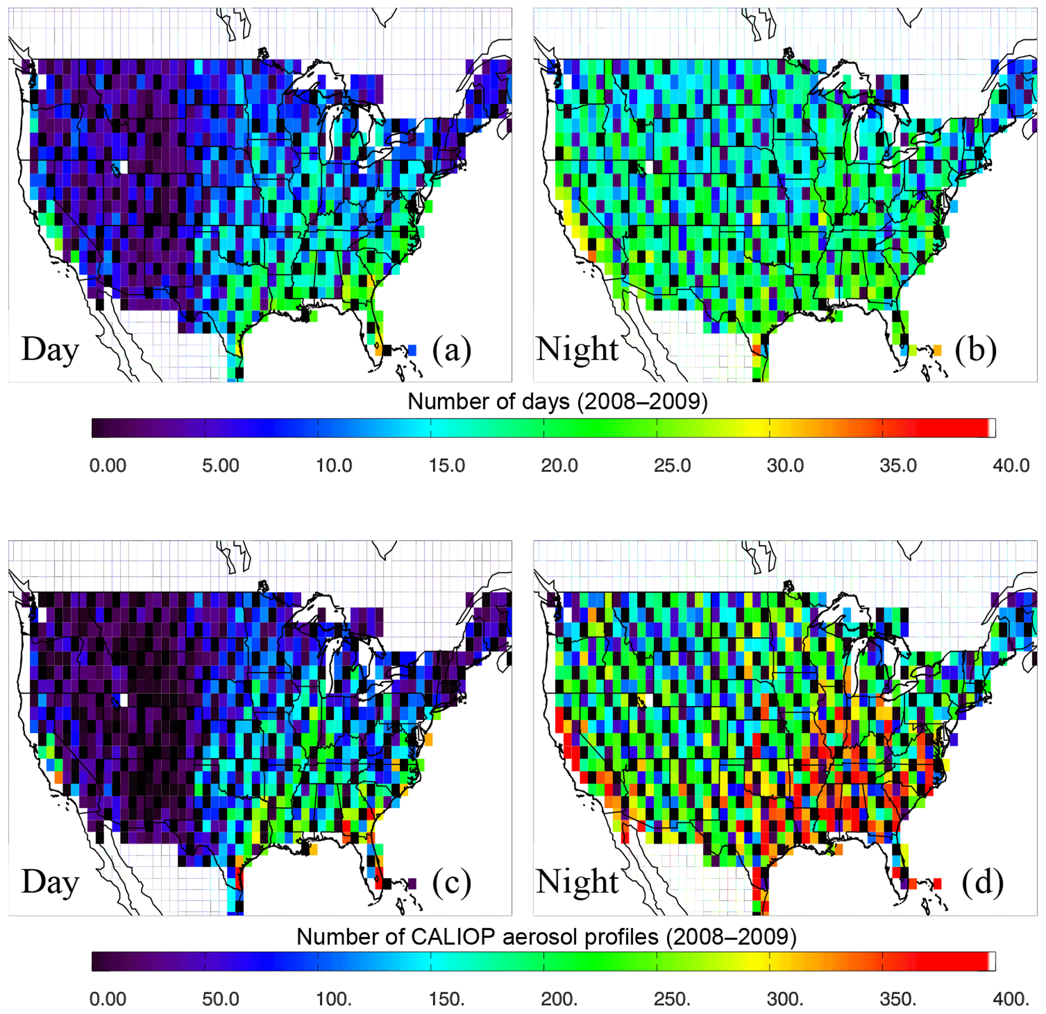
Figure A1 For 2008–2009 over the CONUS, for each 1^∘ × 1^∘ grid box, the number of days and CALIOP Level 2 5 km aerosol profiles used in the creation of the maps in Fig. 3 for (a, c) daytime and (b, d) nighttime measurements. Values greater than 400 profiles for (c, d) are colored red.