the Creative Commons Attribution 4.0 License.
the Creative Commons Attribution 4.0 License.
 | 29 Mar 2019
Cloud products from the Earth Polychromatic Imaging Camera (EPIC): algorithms and initial evaluation
Kerry Meyer
Galina Wind
Yaping Zhou
Alexander Marshak
Steven Platnick
Qilong Min
Anthony B. Davis
Joanna Joiner
Alexander Vasilkov
David Duda
Wenying Su
This paper presents the physical basis of the Earth Polychromatic Imaging Camera (EPIC) cloud product algorithms and an initial evaluation of their performance. Since June 2015, EPIC has been providing observations of the sunlit side of the Earth with its 10 spectral channels ranging from the UV to the near-infrared. A suite of algorithms has been developed to generate the standard EPIC Level 2 cloud products that include cloud mask, cloud effective pressure/height, and cloud optical thickness. The EPIC cloud mask adopts the threshold method and utilizes multichannel observations and ratios as tests. Cloud effective pressure/height is derived with observations from the O2 A-band (780 and 764 nm) and B-band (680 and 688 nm) pairs. The EPIC cloud optical thickness retrieval adopts a single-channel approach in which the 780 and 680 nm channels are used for retrievals over ocean and over land, respectively. Comparison with co-located cloud retrievals from geosynchronous earth orbit (GEO) and low earth orbit (LEO) satellites shows that the EPIC cloud product algorithms are performing well and are consistent with theoretical expectations. These products are publicly available at the Atmospheric Science Data Center at the NASA Langley Research Center for climate studies and for generating other geophysical products that require cloud properties as input.
- Article
(3745 KB) - Full-text XML
- BibTeX
- EndNote


Since June 2015, the Earth Polychromatic Imaging Camera (EPIC) aboard the Deep Space Climate Observatory (DSCOVR) has been providing observations of the sunlit side of the Earth at the L1 Lagrangian point approximately 1.5 million km from the Earth. The simultaneous coverage of the Earth from sunrise to sunset is a capability not previously available from any other spacecraft or Earth observing platform. These observations provide new opportunities in climate research and applications (e.g., Marshak et al., 2018; Holdaway and Yang, 2016a, b). One important contribution of EPIC is the ability to observe and retrieve key radiative properties of clouds, which are of critical importance for understanding the current climate system and for predicting climate change (e.g., Boucher et al., 2013, and references therein). The Decadal Survey for Earth Science and Applications from Space (National Academies of Sciences, Engineering, and Medicine, 2018) lists “how changing cloud cover and precipitation will affect climate, weather, and Earth's energy balance in the future” as one of the key science questions and places the observation of clouds and precipitation on the priority list. Equipped with 10 spectral channels ranging from the UV to the near-infrared, EPIC observations provide essential information for cloud system monitoring and cloud product development.
The focal plane of the EPIC system is a 2048 pixel × 2048 pixel CCD array. The point spread function of the CCD array has a full width at half maximum (FWHM) of ∼1.34 pixels. Images for the 10 spectral channels are obtained using a 10-color filter wheel assembly and shutter, the operation of which takes about 7 min to acquire a complete set of observations. As shown in Fig. 1, the observation starts with the 443 nm channel, followed by the 551, 688, 680, 764, 780, 388, 340, 325, and 317 nm channels. The time difference between one channel and the next consists of readout, exposure, and filter rotation time. Limited by data transmission capability, only the 443 nm channel image is downlinked at its original size; the rest are all reduced to 1024 pixels × 1024 pixels through onboard processing and then interpolated back to the full size of 2048 pixels × 2048 pixels after being downlinked. As can be seen from Fig. 1, the observation time difference between one channel and the next is usually half a minute, except between the 443 and 551 nm, which is ∼3 min. At full resolution, the pixel size of EPIC observations is ∼8 km at nadir. For view zenith angle (VZA) > 0, the EPIC pixels become elliptical, whereby the longer axis increases by a factor of about 1∕cos (VZA) and the shorter axis remains ∼8 km.
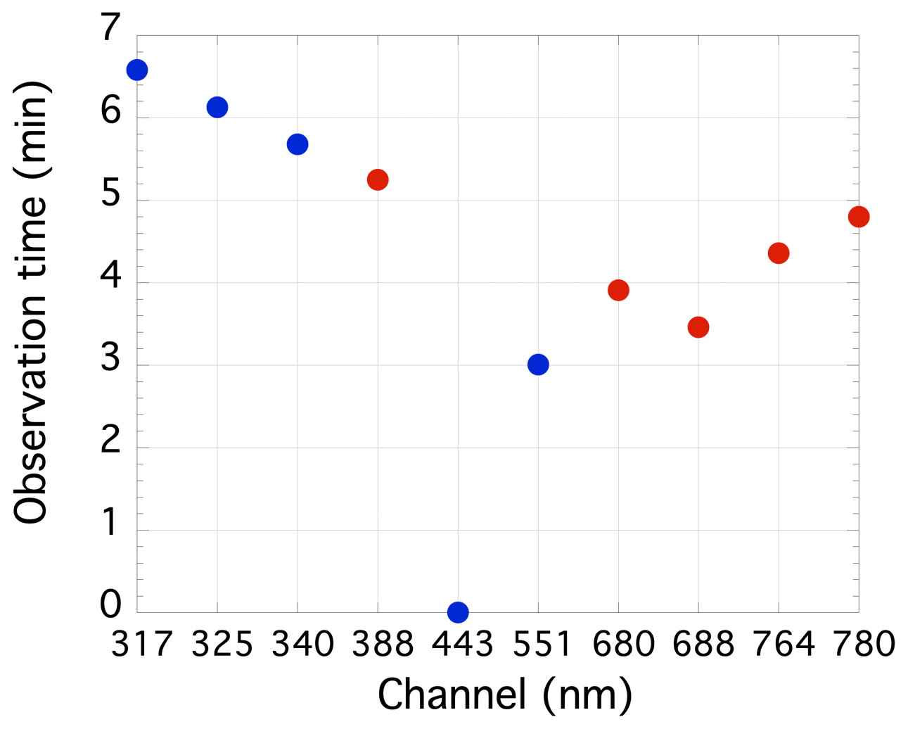
Figure 1Observation time from the start of acquisition for each EPIC channel starting from 443 nm. Red dots are the channels used for cloud retrievals. It takes about 7 min to complete the 10-channel image set.
Due to the latency between imaging different wavelengths and the rotation of the Earth, the regions covered by the images of the 10 EPIC spectral channels are not exactly the same. For algorithm development and research, all 10 spectral channels are projected to a common grid in the Level-1B (L1B) radiance product. The projection procedure includes (see details in Marshak et al., 2018) (1) mapping the images to a 3-D model of the Earth in order to calculate the geolocation of each pixel and (2) projecting and regridding each image onto the common reference grid.
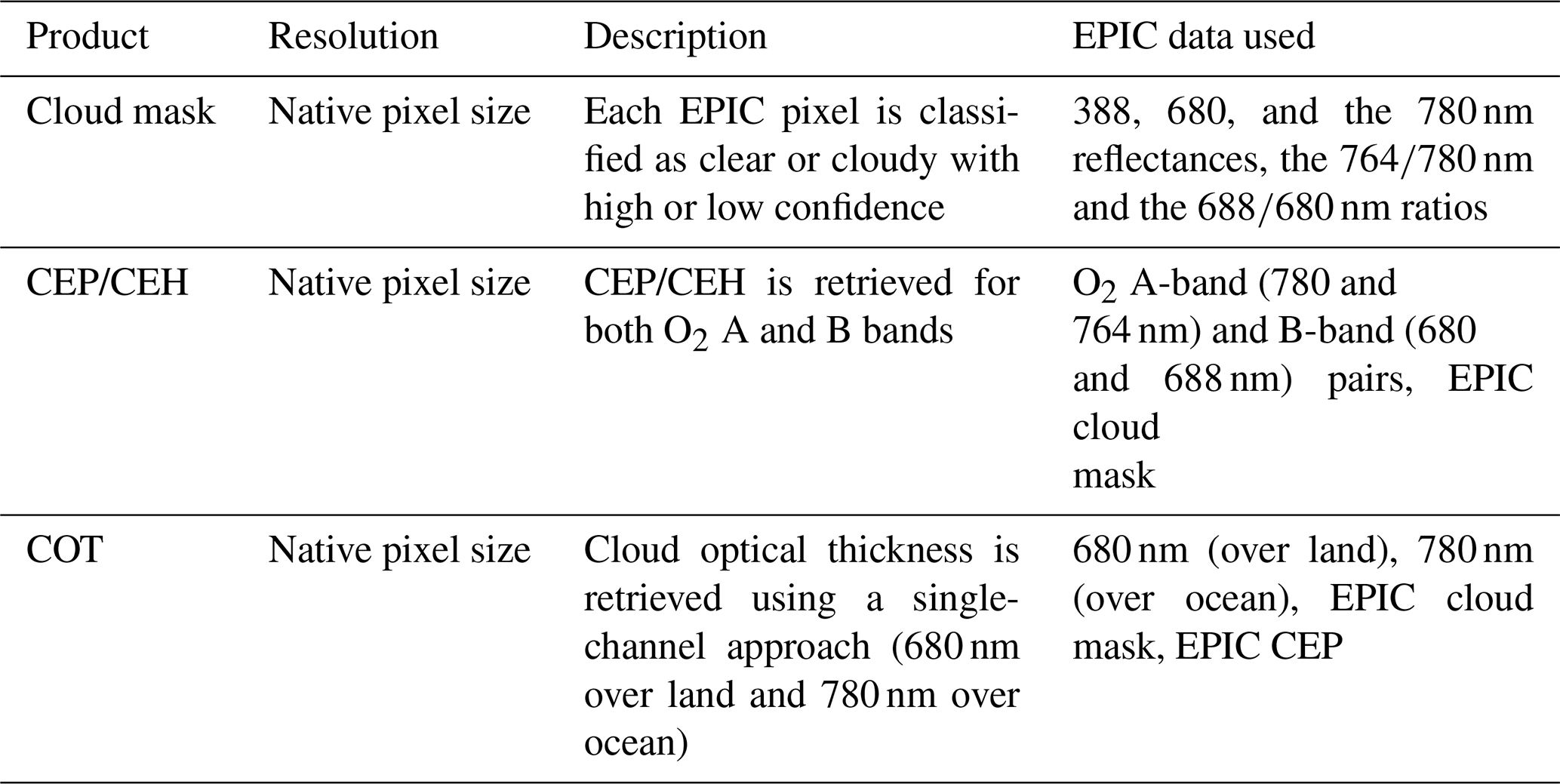
A suite of algorithms has been developed for generating the standard EPIC Level 2 cloud products that include cloud mask, cloud effective pressure/height (CEP/CEH), and cloud optical thickness (COT). These algorithms use as input the observations from five EPIC channels, namely the 388 nm and the two pairs of O2 A-band (780 and 764 nm) and B-band (680 and 688 nm) reference and absorption channels. These observations provide the most cloud information content and are close to each other in observation time, which is important for reducing uncertainties resulting from temporal changes in clouds and the rotation of the Earth. Table 1 gives a summary of the EPIC L2 cloud products. These products, which are publicly available at the Atmospheric Science Data Centre at the NASA Langley Research Center, provide cloud properties of the sunlit side of Earth and are being used in applications such as cloud screening for aerosol property retrievals, ocean color studies, and trace gas retrieval corrections.
Table 1List of current EPIC cloud products and required EPIC observations. The native EPIC pixel size is roughly 8 km at nadir.
The remainder of the paper is organized as follows: Sect. 2 presents the algorithm theoretical basis for the standard EPIC L2 cloud products; Sect. 3 presents an initial assessment of the performance of these products through comparison with results from co-located geosynchronous earth orbit (GEO) and low earth orbit (LEO) observations; a summary and discussions are presented in Sect. 4.
The three components of the EPIC cloud product system, cloud mask, CEP/CEH retrieval, and COT retrieval are run independently. The EPIC cloud mask serves as input to both the CEP/CEH and COT retrievals, for which only pixels classified as cloudy are processed.
2.1 EPIC cloud mask algorithm
The basis for cloud detection is the contrast between cloud and the background surface. To separate cloudy and clear pixels, satellite missions usually adopt the threshold method, which classifies a pixel through comparing the values of an observed quantity, such as the bidirectional reflectance factor (BRF), to a predefined threshold (e.g., Ackerman et al., 2010; Yang et al., 2007; Rossow and Garder, 1993). Moreover, multiple thresholds can be defined such that the cloud mask is assigned a confidence level. Similarly, the goal of the EPIC cloud mask is to label each pixel as clear with high confidence, clear with low confidence, cloudy with low confidence, or cloudy with high confidence. Because EPIC observations are limited to the shortwave channels, the widely used infrared-based tests (e.g., temperature contrast) are not available. However, effective tests can still be constructed. To do that, the Earth's surface is separated into three types: land, ocean, and snow/ice; two tests are applied to each surface type. Table 2 lists the EPIC cloud detection tests used for each surface type.
The two tests used in the EPIC cloud mask over snow-/ice-free land are the 388 nm BRF and the EPIC O2 A-band ratio, i.e., R764∕R780, where R764 is the 764 nm absorption channel BRF and R780 the 780 nm reference channel BRF.
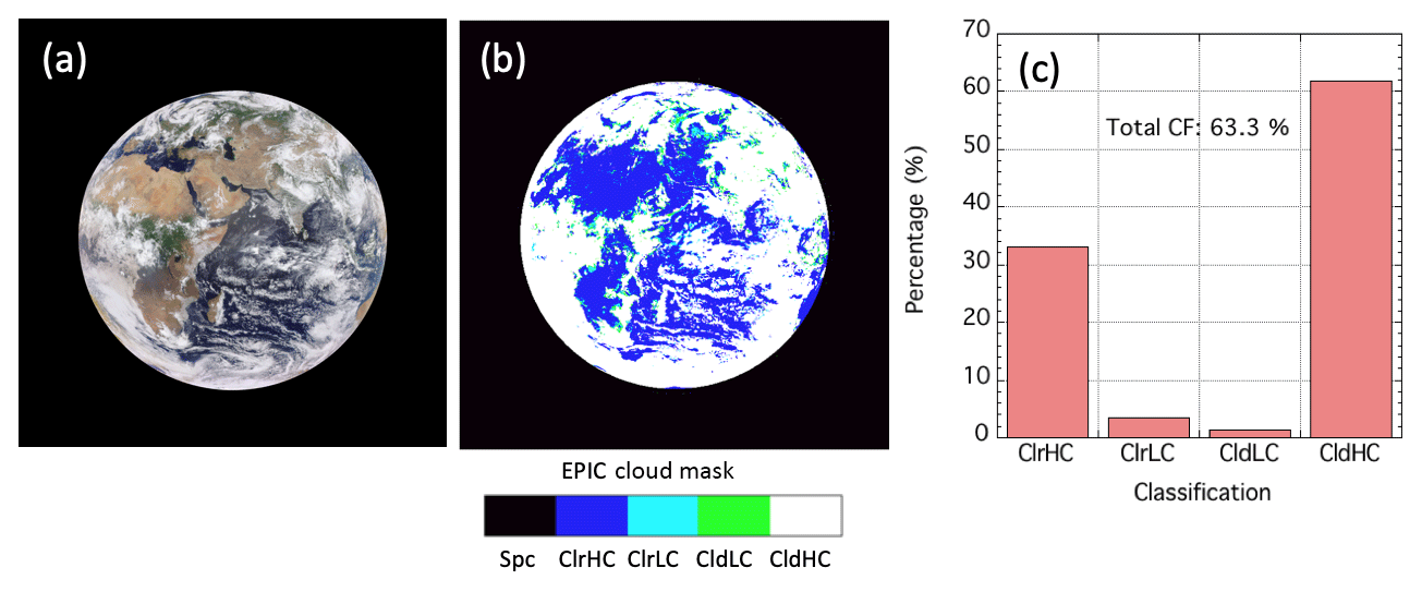
Figure 2Sample EPIC L2 cloud products for the observations at 08:00 UTC on 18 August 2016: (a) EPIC RGB image and (b) EPIC cloud mask. Spc: space pixels, ClrHC: clear with high confidence, ClrLC: clear with low confidence, CldLC: cloudy with low confidence, and CldHC: cloudy with high confidence. (c) Percentage of each scene type derived from the cloud mask.
The utility of the 388 nm channel for cloud detection is due to the fact that surface reflectance in this channel is usually small, while clouds are relatively bright over snow-/ice-free land (Herman et al., 2001). To accommodate a wide range of sun-view geometries, the contribution from Rayleigh scattering is first removed from the observed BRF. A truly accurate Rayleigh correction requires knowledge of the reflecting layer height and its microphysical properties. However, for the more qualitative purposes of cloud detection, we can apply a simple Rayleigh correction based on the assumption that the observed reflectance comes from the interaction of a Lambertian surface and a Rayleigh layer above. Then the derived Lambertian-equivalent reflectivity (LER) (e.g., Herman and Celarier, 1997) can be compared with the surface albedo to decide if clouds are present. The EPIC observed BRF at the top of atmosphere (TOA) RTOA can be expressed as
where RLER is the Lambertian-equivalent reflectivity to be derived; RR, TR, and SR are the Rayleigh path reflectance, two-way transmittance, and spherical albedo, respectively, which are calculated with the analytical solutions described in Vermote and Tanre (1997). Thresholds for the 388 nm test are based on the monthly surface reflectance climatology derived from the Global Ozone Monitoring Experiment-2 (GOME-2) and the SCanning Imaging Absorption SpectroMeter for Atmospheric CHartographY (SCIAMACHY) missions (Tilstra et al., 2017). In practice, if the Rayleigh corrected LER is larger than the surface albedo, then the scene is labeled as cloudy; otherwise, it is clear. The uncertainty in the surface albedo provided by the dataset (Tilstra et al., 2017) is used to decide the confidence level.
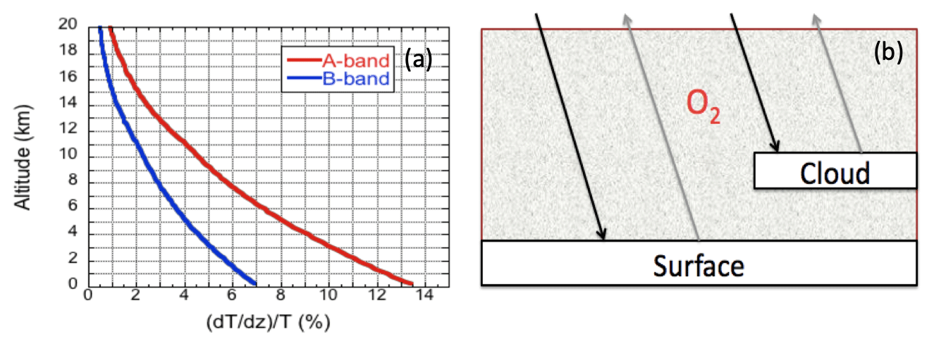
Figure 3(a) Derivative of the clear sky two-way transmittance (dT∕dz) for the EPIC A- and B-band absorption channels normalized by T, where T is the two-way transmittance and z is the height. The plot shows how much T changes (%) if the altitude of the reflecting layer changes by 1 km. (b) The two types of photon paths considered in the MLER method. The picture shows one partially cloudy EPIC pixel.
The selection of the O2 A-band ratio as a cloud mask test is based on the fact that everything being equal, the ratio is higher with the presence of clouds compared to clear sky cases because O2 absorption is proportional to the air mass above the reflecting layer. Thresholds for this test are a function of surface elevation, which is based on the Global Gridded Elevation and Bathymetric (ETOPO5) dataset (Edwards, 1989). While the O2 B-band ratio is also useful for cloud detection for the same reason (and is used over snow/ice as discussed below), the A-band ratio is selected for use over land because it provides better skill than that of the B band due to its higher sensitivity to the photon path length change (Y. Yang et al., 2013).
Over ocean, the BRFs of the 680 and the 780 nm channels are used for cloud detection because clouds and the sea surface contrast well in both channels. Although the observations are highly correlated, the two channels complement each other over coastal and shallow water regions due to differences in surface reflectance. Similar to the 388 nm test over land, a Rayleigh correction is also applied to both the 680 and 780 nm BRFs. Thresholds are derived empirically. BRF values RT680=0.11 and RT780=0.10 are used to separate low confidence clear and low confidence cloudy scenes for the 680 and 780 nm channels, respectively. RT680±0.03 and RT780±0.03 are used as the high confidence thresholds for the two channels, respectively.
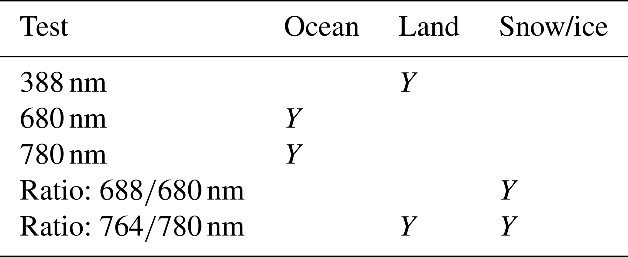
Over snow- and ice-covered regions, both the O2 A- and B-band ratios are used for cloud detection. As discussed above for the A-band ratio test over land surfaces, the relative shorter photon path lengths under cloudy conditions result in higher ratios. The thresholds are selected based on radiative transfer simulations with the Discrete Ordinates Radiative Transfer model (DISORT) (Stamnes et al., 1988). Unless otherwise mentioned, the radiative properties of the atmosphere at the A and B band used in this paper are calculated with the Line-By-Line Radiative Transfer Model (LBLRTM) (Clough et al., 2005) using the 1976 U.S. Standard Atmosphere, and monochromatic radiative transfer results were convolved with the filter functions. Detailed properties of the EPIC A- and B-band channels are described in Y. Yang et al. (2013).
The procedure of generating the EPIC cloud mask includes two steps. First, for a given surface type, each of the two tests leads to an independent cloud mask represented with an integer value:
Second, the final cloud mask is assigned based on the sum of the individual tests, such that
Figure 2 shows an example of the EPIC cloud mask for the observations at 08:00 UTC on 18 August 2016. As can be seen from the figure, the EPIC cloud mask (Fig. 2b) matches the corresponding RGB (Fig. 2a) well. The fraction of the four scene types, i.e., clear with high confidence (ClrHC), clear with low confidence (ClrLC), cloudy with low confidence (CldLC), and cloudy with high confidence (CldHC), are 33.1 %, 3.6 %, 1.4 %, and 61.9 %, respectively. From the cloud mask, it is straightforward to derive Earth's daytime cloud coverage (Fig. 2c); for this granule, the total cloud coverage, including cloudy with low and high confidence, is 63.3 %.
2.2 EPIC CEP/CEH algorithm
The EPIC CEP/CEH is derived from observations in the O2 A-band (780 and 764 nm) and B-band (680 and 688 nm) pairs. The idea of using O2 absorption for cloud height retrieval has been investigated extensively and has been implemented in several operational algorithms (e.g., Loyola et al., 2018; Schüssler et al., 2014; Ferlay et al., 2010; Davis et al., 2009; Vasilkov et al., 2008; Wang et al., 2008; Lindstrot et al., 2006; Kokhanovsky et al., 2005; Min et al., 2004; Vanbauce et al., 2003; Daniel et al., 2003; Koelemeijer et al., 2001; Stephens and Heidinger, 2000; Buriez et al., 1997). With the O2 A- and B-band observations, EPIC provides an unprecedented opportunity to monitor cloud height from the L1 point. An information content analysis on EPIC A- and B-band observations is provided in Davis et al. (2018a, b).
Figure 3a shows the sensitivity of the EPIC A and B bands to the reflecting layer height change, represented here by the derivative of the above-cloud two-way transmittance (T) with respect to height (z). While the A band has stronger absorption than the B band, the sensitivity to cloud height is clear for both channels. For example, perturbing by 1 km the altitude of a reflecting layer at 5 km changes the atmosphere two-way transmittance by ∼8 % for the A band and ∼4 % for the B band.
Since oxygen is a well-mixed gas, it would be easy to derive cloud top height from radiance measurements in the absorption band if the cloud behaved optically like a hard target. However, multiple scattering along the photon path inside and outside the cloud complicates the situation. Due to photon penetration into the cloud, for given optical thickness and particle properties, the radiance measured by the EPIC A- and B-band sensors is not only a function of cloud top height, but also a function of cloud extinction coefficient profile. Except under special situations, e.g., for optically thick clouds over dark surfaces with vertically uniform extinction coefficient (Y. Yang et al., 2013), the EPIC measurements generally do not provide enough information content to retrieve the actual cloud top, but they are sufficient for retrieving another important cloud location information – namely CEP/CEH, as well as the effective cloud fraction (ECF).
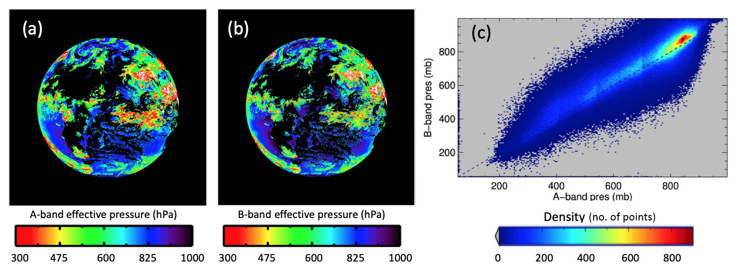
Figure 4Sample EPIC L2 cloud effective pressure (CEP) products. Same granule as Fig. 3, but for (a) O2 A-band CEP, (b) O2 B-band CEP, and (c) scatterplot for A- vs. B-band CEP.
CEP is equivalent to the mean pressure from which light is scattered and ECF is the derived radiometrically equivalent cloud fraction assuming an a priori cloud albedo (Stammes et al., 2008). CEP and ECF are important information, and both have been widely applied to trace gas retrievals and climate studies (e.g., Joiner et al., 2012; Wang et al., 2011; Vasilkov et al., 2008; Stammes et al., 2008; Sneep et al., 2008). CEP and ECF are retrieved using the Mixed Lambertian-Equivalent Reflectivity (MLER) concept, which has been extensively studied and applied to operational settings (e.g., Joiner et al., 2012; Y. Yang et al., 2013; Koelemeijer et al., 2001). The MLER model assumes that the pixel contains two Lambertian reflectors, the surface and the cloud. Figure 3b illustrates the concept. The cloud is assumed to be opaque; hence photon transmission is neglected. The reflectance observed at the sensor can be expressed as
where Rabs and Rref are the observed reflectances for the absorption and the reference channels, respectively, Ac is the ECF, αs is the surface albedo, αc is the a priori cloud albedo, Tabs and Tref are the two-way atmospheric transmittances for the absorption and the reference channels, respectively, Pc and Ps are the CEP and the surface pressure, respectively, and θ and θ0 are the view zenith and solar zenith angles, respectively. Generally, αc is assumed to be 0.8, which corresponds to an optically thick cloud. This value is selected to justify the no transmission assumption of the MLER model. It has been demonstrated that although the selection of the a priori cloud albedo does affect the results of the ECF, its effect on the retrieved CEP is relatively small (Stammes et al., 2008; Koelemeijer et al., 2001).
CEP and ECF can be retrieved with Eqs. (4) and (5) through iteration, after which CEP is converted to cloud effective height (and, in the COT retrieval, cloud effective temperature; see Sect. 2.3) using co-located atmospheric profiles provided by the Goddard Earth Observing System Model, Version 5 (GEOS-5) (Lucchesi, 2015). The retrieval of CEP only requires one pair of absorption and reference channel observations; hence two independent EPIC CEPs can be obtained using the A-band and B-band pairs. In theory, the two CEPs are very close to each other if the surface albedo is the same for the two bands and instrument noise is not considered. There exists a subtle difference between the two CEPs, however, because of the difference in photon penetration depths, which contains information on cloud vertical structure (Y. Yang et al., 2013). Due to weaker absorption, photons in the B band penetrate deeper into the cloud and result in a slightly higher CEP (lower altitude). As a result, both the A- and B-band CEPs are reported in the EPIC cloud product for the community to explore. For applications that need specific cloud effective height, such as trace gas retrieval correction, the A-band value is recommended as it is less noisy. Figure 4a and b show the two CEP retrievals for the same granule as in Fig. 2. As can be seen from the scatterplot in Fig. 4c, the A- and B-band CEPs are generally close to each other, with the B-band CEP higher. From radiative transfer simulations, the differences between the two CEPs resulting from penetration depth difference should be small (Y. Yang et al., 2013; Davis et al., 2018a, b). In addition, potential instrument instability, surface albedo differences, calibration accuracy, and changes resulting from the differences in observation time (see Fig. 1) can also cause differences in the two CEPs.
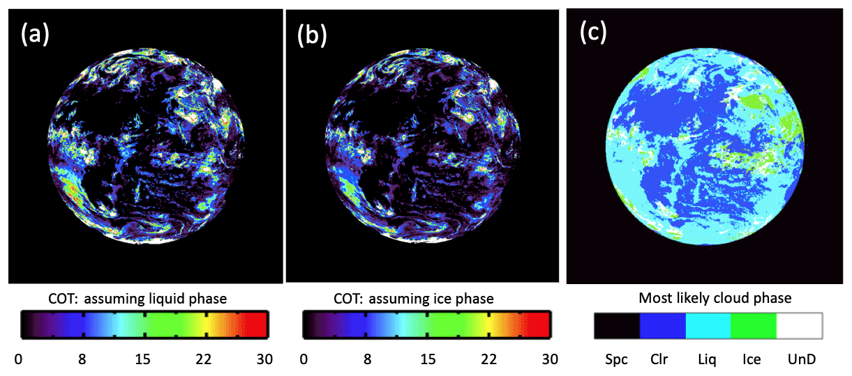
Figure 5Sample EPIC L2 cloud optical thickness (CODT) products. Same granule as Fig. 3, but for (a) COT retrieval assuming liquid thermodynamic phase, (b) COT retrieval assuming ice thermodynamic phase, and (c) the most likely cloud phase based on cloud effective temperature derived from the A-band CEP.
2.3 EPIC COT algorithm
Simultaneously retrieving COT and cloud effective radius (CER) using a combination of absorbing and non-absorbing spectral channels has been common practice (e.g., Platnick et al., 2017; Nakajima and King, 1990). However, due to the lack of a particle-size-sensitive absorbing shortwave/mid-wave infrared channel, the EPIC COT retrieval adopts a single-channel approach similar to what has been used by the International Satellite Cloud Climatology Project (ISCCP) (Rossow and Schiffer, 1999), the Multi-angle Imaging SpectroRadiometer (MISR) mission (Marchand et al., 2010), and the Geoscience Laser Altimeter System (GLAS) solar background application project (Yang et al., 2008). The 780 and 680 nm channels are used for retrievals over ocean and over land, respectively. Fixed particle sizes are assumed based on the MODIS global cloud effective radius modes derived from the Collection 6 (C6) MODIS cloud products (14 µm for liquid clouds and 30 µm for ice clouds). Using MODIS data, it has been shown that the uncertainties for a single-channel retrieval due to assuming a fixed cloud effective radius are roughly 10 % for liquid clouds and 2 % for ice clouds (Meyer et al., 2016).
The EPIC COT algorithm shares the same code base, forward model assumptions, and, to the extent possible, ancillary usage as the current C6/C6.1 MODIS cloud optical/microphysical property retrievals (MOD06) (Platnick et al., 2017). Since EPIC does not provide enough information to confidently determine cloud thermodynamic phase, two COT values are retrieved and reported for each cloudy pixel by assuming liquid and ice phases, respectively. A similar approach has been used by Chiu et al. (2010). Nevertheless, by combining the A- and B-band CEPs and GEOS-5 atmospheric profiles, the EPIC cloud product also provides A- and B-band cloud effective temperatures as well as a most likely cloud thermodynamic phase derived from thresholds applied to the A-band CEP and temperature. Providing two COT values is useful to the community for further synergistic research, when more information on cloud phase is available from other sources. An example of EPIC COT and the most likely cloud phase product is shown in Fig. 5 for the same granule as in Fig. 2.
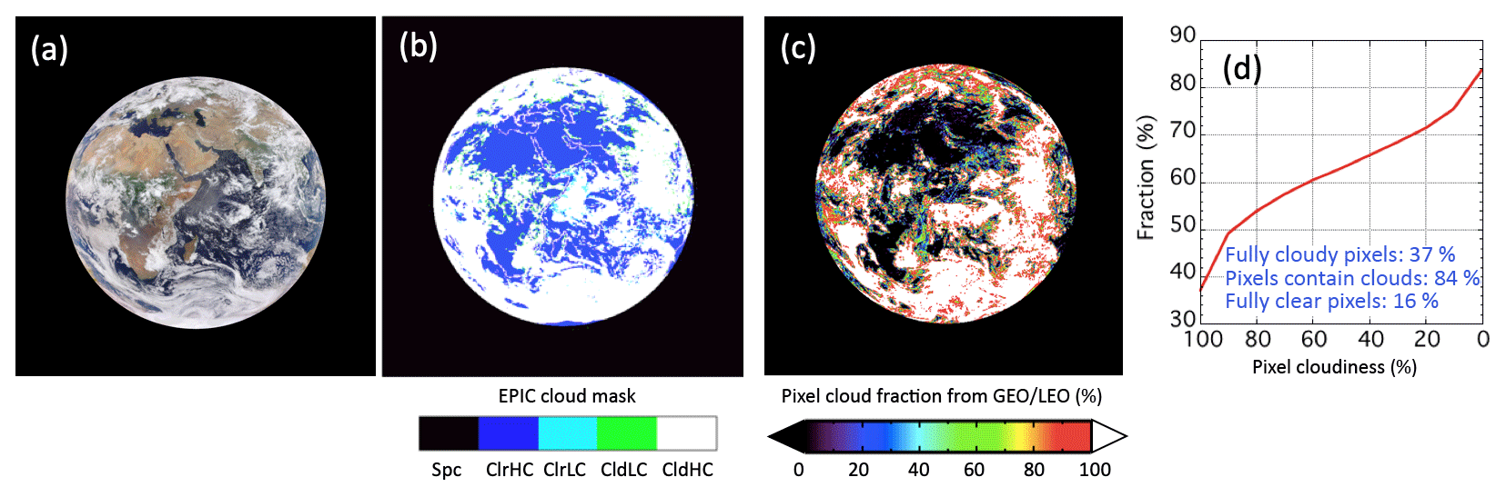
Figure 6Comparison of the EPIC cloud mask with the co-located GEO–LEO satellite results. (a) The EPIC RGB image for 08:00 UTC on 15 September 2015, (b) the corresponding EPIC cloud mask, (c) the corresponding GEO–LEO composite for the sub-pixel cloud fraction of each EPIC pixel, and (d) the cumulative distribution of pixels from 100 % cloudy to fully clear for this granule based on the GEO–LEO composite in (c).
An initial performance assessment has been conducted by comparing the EPIC cloud products with co-located cloud retrievals from GEO–LEO satellites. A GEO–LEO composite dataset has been generated by the Clouds and the Earth's Radiant Energy System (CERES) team at the NASA Langley Research Center by projecting the GEO–LEO retrievals to the EPIC grid (Khlopenkov et al., 2017). This composite dataset is produced in a two-step process to convert LEO and GEO data into an EPIC-view perspective. An algorithm for optimal merging of selected radiances and cloud properties derived from multiple satellite imagers produces nearly seamless global composites at a fixed 5 km resolution at each EPIC observation time. The composite data are subsequently remapped into the EPIC-view domain by convolving composite pixels with the EPIC point spread function (PSF) defined with a half-pixel accuracy. PSF-weighted average radiances and cloud properties are computed separately for each cloud phase. The merging process uses the GEO–LEO measurements nearest to the EPIC observation time to create the composite. The GEO platforms used include the Geostationary Operational Environmental Satellites (GOES), the MeteoSat satellites, the Multifunctional Transport Satellites (MTSAT), and the Himawari-8 satellites. The LEO sensors used include MODIS on NASA's Terra and Aqua and AVHRR on NOAA's satellites. The retrieval and projection methods used are described in Minnis et al. (2011) and Khlopenkov et al. (2017). We note that the retrievals from the GEO–LEO platforms have uncertainties as well, but this dataset serves as an independent source for the assessment and consistency check of the EPIC cloud products.
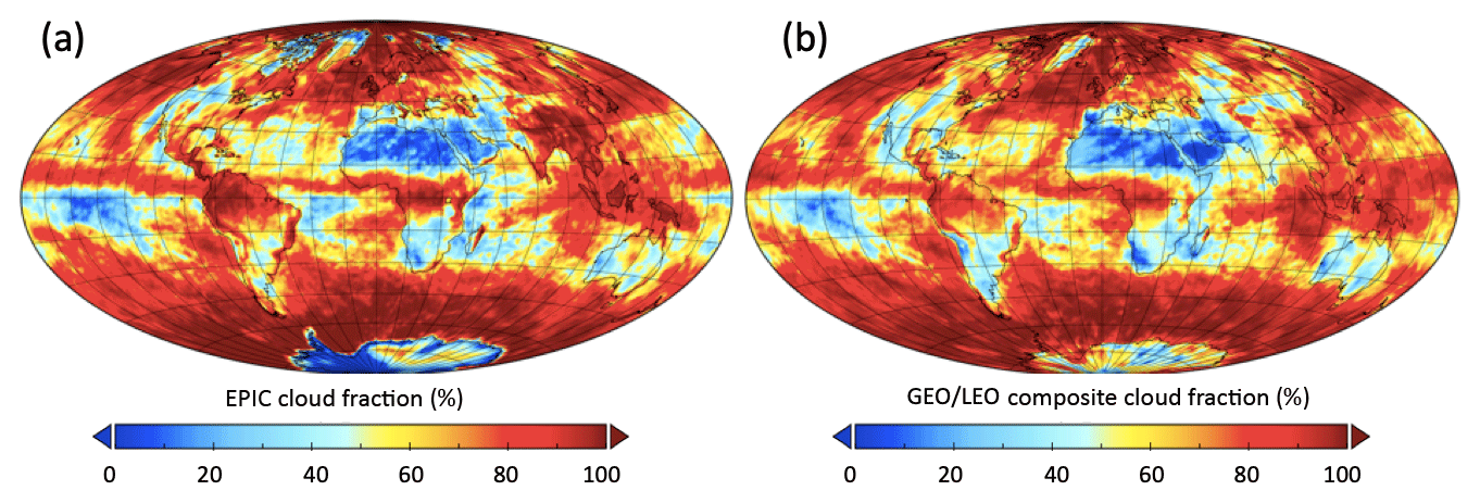
Figure 7Comparison between EPIC global cloud coverage and co-located (spatially co-located and time difference within 5 min) GEO–LEO results. Four weeks of data from 2016 are utilized with 1 week from each season (6–12 March, 20–26 June, 21–27 September, and 20–26 December). (a) Average EPIC cloud coverage and (b) average cloud coverage from the GEO–LEO composites.
With the performance assessment, we also attempt to provide an uncertainty estimate for the EPIC cloud products. Retrieval uncertainty can come from many sources, including the assumptions and simplifications in the retrieval algorithm, instrument calibration, geolocation inaccuracy, and cloud evolution within the latency between imaging different wavelengths. Note that pixel-level uncertainties of the COT retrievals, accounting for known and quantifiable error sources including radiometry, ancillary atmospheric profile, surface spectral reflectance, cloud forward model, and cloud effective radius assumptions, are provided in the current version of the operational products (Meyer et al., 2016; Platnick et al., 2017); uncertainty for other products will be included in the next version.
3.1 Performance of EPIC cloud mask
Since the data from the GEO–LEO satellite instruments have finer spatial resolutions than EPIC, each EPIC pixel is likely to contain many GEO–LEO instrument pixels; hence a sub-pixel cloud fraction can be calculated for each co-located EPIC pixel. Figure 6 shows an example. Comparing the EPIC RGB image (Fig. 6a) with the corresponding cloud mask (Fig. 6b), it can be seen that the EPIC cloud mask performs well for this case. Figure 6c is the corresponding sub-pixel cloud fraction for each EPIC pixel from the GEO–LEO composite. From the cumulative distribution of the GEO–LEO composite in Fig. 6d, 37 % of the EPIC pixels are fully cloudy and 16 % are fully clear; the remainder (84 %) of the EPIC pixels have some level of partial cloudiness. The EPIC cloud mask gives a cloud fraction for the entire scene of 66.4 %. While we re-emphasize that a portion of the EPIC pixels are only partially cloudy, the comparison between the global cloud coverage derived from EPIC and from the GEO–LEO composite is still meaningful in understanding the performance of the EPIC cloud mask.
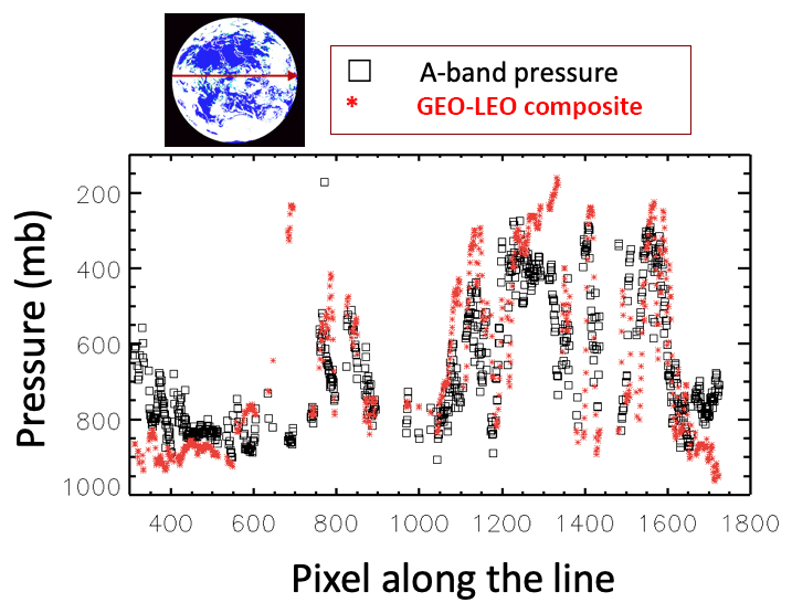
Figure 8Comparison of EPIC A-band CEP with the co-located GEO–LEO retrievals for the same granule as Fig. 6. The comparison is done along the red arrow shown on the cloud mask thumbnail at top.
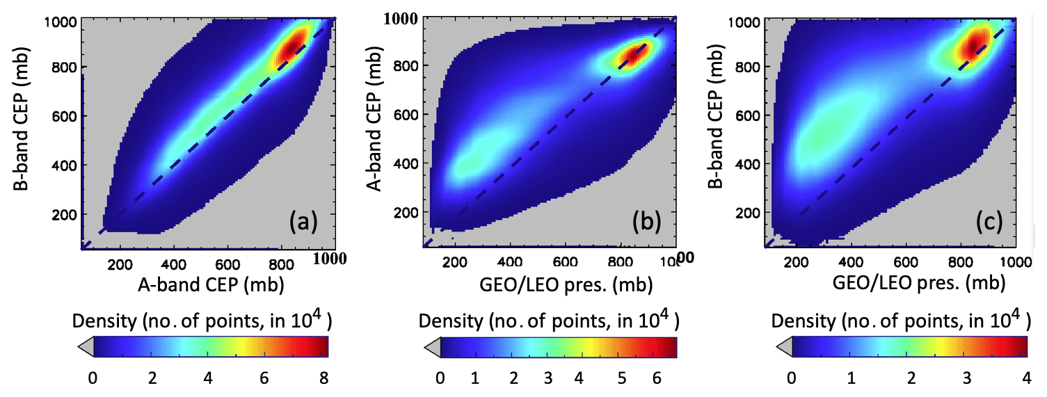
Figure 9EPIC A- and B-band CEP and the comparison with cloud pressure from GEO–LEO composites. Data used are the same as in Fig. 7. Scatterplots (a) for EPIC A- vs. B-band CEP, (b) the GEO–LEO composites cloud pressure vs. EPIC A-band CEP, and (c) the GEO–LEO composites cloud pressure vs. EPIC B-band CEP.
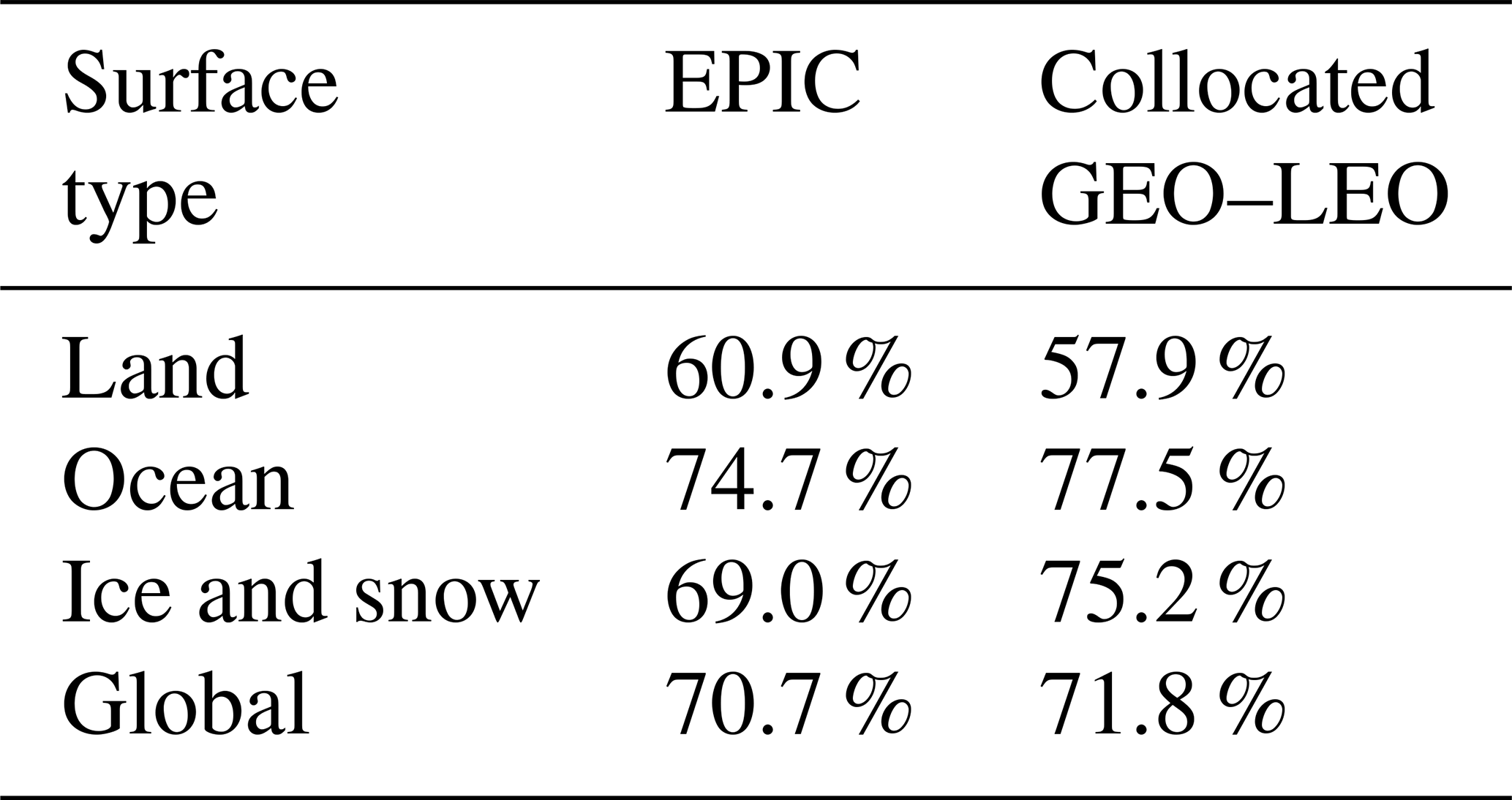
Figure 7 compares the global average cloud fraction from EPIC and from the GEO–LEO composites from 4 weeks of data, one from each season, in 2016 (6–12 March, 20–26 June, 21–27 September, and 20–26 December). Cloud fractions are calculated for each 1∘ × 1∘ latitude–longitude grid box. For this study, the global statistics are done with a customized version of the composites that uses only GEO–LEO data within ±5 min of the EPIC observation time to minimize the temporal differences between the EPIC and GEO–LEO data. As shown in the figure, the two datasets visually match each other well. The total global cloud fractions are 70.7 % and 71.8 % for EPIC and the GEO–LEO composites, respectively (Table 3). Over land it is 60.9 % for EPIC and 57.9 % for GEO–LEO; over ocean it is 74.7 % for EPIC and 77.5 % for GEO–LEO. Discrepancies exist between the two datasets; the most obvious one is over snow- and ice-covered regions. For example, EPIC misses a large portion of clouds over West Antarctica, where cloud detection uses the O2 A- and B-band ratios. Ongoing efforts are taking place to improve cloud masking performance over these regions.
Table 3Comparison between EPIC cloud fraction and collocated GEO–LEO results. Data used are the same as in Fig. 7.
To further quantify the uncertainty in the cloud mask, we use the GEO–LEO composites as the reference and calculate the accuracy, the percentage of correct detection (POCD), and the percentage of false detection (POFD):
where α, β, χ, and γ are the number of pixels corresponding to the following scenarios: (1) both the EPIC cloud mask and the GEO–LEO composite identify as cloudy; (2) both identify as clear; (3) EPIC identifies as clear, but the composite identifies as cloudy; and (4) EPIC identifies as cloudy, but the composite identifies as clear, respectively. Note that we count both the low and high confidence cloudy pixels in the EPIC cloud mask as cloudy. For the GEO–LEO composites, we consider pixels with a cloud fraction greater than 50 % as cloudy. Since the EPIC cloud mask has known issues over ice sheets, which are being worked on, we excluded ice sheets in the calculations. Results show that using the GEO–LEO composites as a reference, accuracy is 82.4 %, POCD 88.7 %, and POFD 13.1 %.
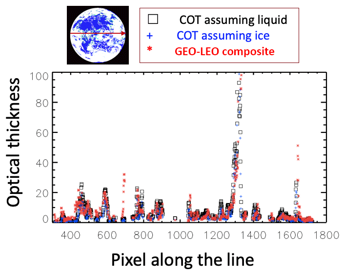
Figure 10Comparison of EPIC COT with the collocated GEO–LEO retrievals for the same granule as in Fig. 6. The comparison is done along the red arrow shown on the cloud mask thumbnail at top.
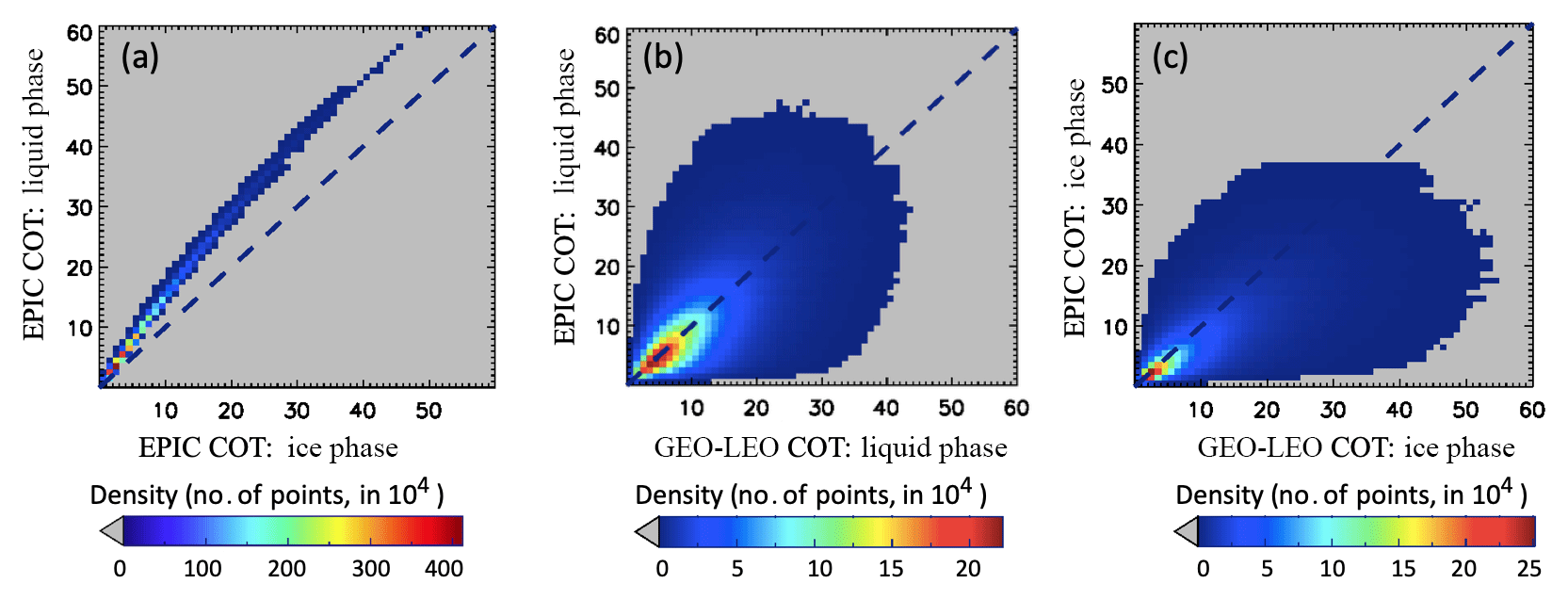
Figure 11(a) Scatterplot for EPIC COT assuming liquid vs. ice phase; (b) EPIC COT vs. GEO–LEO composites: liquid clouds only as identified by the GEO–LEO algorithms; and (c) EPIC COT vs. GEO–LEO composites: ice clouds only as identified by the GEO–LEO algorithms. Data used are the same as in Fig. 7.
3.2 Performance of EPIC CEP/CEH
As discussed above, the retrieved CEPs are generally higher (lower altitude) than the physical cloud top pressure due to the photon penetration into clouds that is ignored in the adopted MLER concept. However, at the most oblique solar zenith and view zenith angles, CEPs can be lower (higher altitude) than the physical cloud top due to the contribution of Rayleigh scattering (e.g., Y. Yang et al., 2013; Ferlay et al., 2010; Vanbauce et al., 2003).
Figure 8 compares the EPIC A-band CEP with the GEO–LEO composites. Cloud pressures in the GEO–LEO composite are derived from infrared channels, which are radiative pressures but are closer to the physical cloud top. As shown in the Figure, the EPIC A-band CEPs are generally higher (lower altitude) than those of the GEO–LEO composites (note that the vertical axis is reversed), except at the edges of the image where the solar and view zenith angles are both large. The mean cloud pressures along this line are 658 mb for the EPIC A-band and 645 mb for the GEO–LEO composite. As discussed in Sect. 2.2, the EPIC cloud pressure is essentially the centroid of the reflected photons registered at the satellite sensor. Photons penetrating into and through clouds have longer path lengths compared to photons reflected at the cloud top. Since the LER model does not take these factors into account, it is expected that the EPIC CEP is lower in altitude than the physical cloud top (higher in pressure); hence the results shown here are consistent with previous studies and theoretical predictions.
Figure 9a compares the EPIC A- and B-band CEP retrievals using the same 4 weeks of data as in Fig. 7. Results are similar to the single granule case shown in Fig. 4c. The A- and B-band CEPs are generally close to each other with the B-band CEP higher (lower altitude). The spread of the scatterplot can come from spectral surface albedo differences, changes resulting from the differences in observation time, and calibration accuracy, etc. Figure 9b and c show the comparison between EPIC A- and B-band CEP and cloud pressure from GEO–LEO composites. In general, the GEO–LEO cloud pressure is lower (higher in altitude) than the CEPs, as their sensitivity lies closer to the physical cloud top. The mean differences between the EPIC A-band and B-band CEPs and the GEO–LEO cloud pressure are 92.7 and 147.5 hPa, respectively. Again, the results are consistent with existing studies and theoretical expectations.
3.3 Performance of EPIC COT retrieval
As mentioned above, the EPIC COT retrieval adopts a single-channel approach in which the 780 and 680 nm channels are used for retrievals over ocean and over land, respectively, and the algorithm shares the same code base, forward model assumptions, and ancillary usage as the current MODIS C6/C6.1 cloud optical property products. A separate comprehensive study has been conducted to investigate the feasibility and uncertainty of the EPIC COT retrieval algorithm (Meyer et al., 2016). The study showed that for ice clouds, uncertainties are mostly less than 2 % because even though a fixed particle size is assumed (30 µm), the ice crystal model used in the retrieval (i.e., severely roughened aggregate of hexagonal columns) (P. Yang et al., 2013; Holz et al., 2016) is not sensitive to the particle size; for liquid clouds the uncertainty is larger, roughly 10 %, although for thin clouds (COT < 2) the error can be higher.
Figure 10 shows a comparison of the two EPIC COT retrievals (liquid and ice phase) with the GEO–LEO composites. In general, there is good correlation between the EPIC and GEO–LEO composite COTs. For reference, the mean EPIC COT along the selected line is 8.9 for liquid phase, 7.4 for ice phase, and 9.5 for the GEO–LEO composite. Using the same 4 weeks of data as in Fig. 7, Fig. 11a shows the relationship between the two EPIC COT retrievals by assuming ice and liquid phase, respectively. As expected, for the same reflectance, liquid clouds have higher COT than ice clouds (King et al., 2004). Figure 11b and c compare the EPIC COT with the GEO–LEO COT for liquid and ice phase clouds, as identified by the GEO–LEO retrieval algorithm (Minnis et al., 2011). In general, the two products match each other well. We emphasize again that the COT retrievals used in the GEO–LEO composites are generated by the CERES Cloud team with a different set of assumptions and cloud models (Minnis et al., 2011) than are used in the EPIC COT retrievals. Other factors that can contribute to the spread include the differences in observation time and the instrument spatial resolution.
From the Earth–Sun system L1 Lagrangian point, EPIC has been providing a continuous view of the sunlit side of the Earth since June 2015. Observations from the 10 EPIC spectral channels are a unique dataset for cloud system monitoring and cloud product development. A suite of algorithms has been developed to generate the standard EPIC Level 2 cloud products that include cloud mask, CEP/CEH, and COT. These products are archived at the Atmospheric Science Data Center at the NASA Langley Research Center.
The EPIC cloud product algorithms are presented. The EPIC cloud mask adopts the threshold method and utilizes the BRFs of the 388, 680, and 780 nm channels, the 764 and 780 nm (A-band) ratio, and the 688 and 680 nm (B-band) ratio as tests. The Earth's surface is separated into three types: land, ocean, and snow/ice; two tests are applied to each surface type, and the results from each test are combined to generate the final cloud mask, which classifies a pixel as clear or cloudy with confidence levels. The EPIC CEPs are derived with observations from the O2 A-band (780 and 764 nm) and B-band (680 and 688 nm) pairs based on the MLER model. Both A-band CEP and B-band CEP are reported in the cloud product. CEPs are converted to cloud heights using the co-located atmospheric profiles provided by the GEOS-5 model. Due to the lack of particle size sensitive channels, the EPIC COT retrieval adopts a single-channel approach in which a fixed particle size is assumed. Observations from the 780 and 680 nm channels are used for retrievals over ocean and over land, respectively. In addition, since the EPIC channels do not contain enough information to confidently determine cloud thermodynamic phase, the EPIC COT product provides two independent retrievals for each cloudy pixel, one assuming liquid phase and one assuming ice phase, respectively. A most likely cloud thermodynamic phase is also provided based on thresholds applied to the CEP and the cloud effective temperature derived from the EPIC O2 A band.
An initial comparison with co-located GEO–LEO results shows that the EPIC cloud products are performing well. Based on the analysis of 4 weeks of data from the year 2016, the total global cloud fractions are 70.7 % and 71.8 % for EPIC and the GEO–LEO composites, respectively. Due to photon penetration, the EPIC CEPs are generally higher (lower altitude) compared to the GEO–LEO retrievals from infrared channels that have sensitivity closer to the physical cloud top. The EPIC CEP retrievals are consistent with theoretical expectations. The EPIC COT retrieval shares the same code base, forward model assumptions, and ancillary usage as the current C6/C6.1 MODIS cloud optical/microphysical property retrievals (MOD06).
The EPIC cloud products provide cloud properties of the sunlit side of Earth for climate studies and for generating other geophysical products that require cloud properties as input. Known issues include the cloud detection problems over ice and snow, which lead to errors in CEP/CEH and COT retrievals. Ongoing efforts are taking place to improve the EPIC cloud products in these regions.
The DSCOVR level-1 and level-2 data used in this paper are publicly available from the NASA Langley Atmospheric Sciences Data Center (ASDC).
All authors contributed to planning and writing of the paper. YY initiated and led the EPIC Level 2 cloud product project, designed and implemented the cloud mask and effective pressure/height algorithms, and drafted the paper. KM and GW implemented the EPIC cloud phase and COT retrieval algorithm and conducted cloud product system integration; KM also conducted the EPIC COT retrieval algorithm uncertainty study and contributed to the cloud mask algorithm design. YZ conducted the cloud product assessment, AM initiated and conducted the EPIC cloud height study and provided guidance for the initial design of the cloud height retrieval algorithm, and SP provided access to the MODIS cloud product retrieval infrastructure and provided guidance for modifications to suit the EPIC product needs. QM investigated the derivation of cloud top height from EPIC cloud effective pressure/height retrievals, ABD conducted a two-pronged information content analysis of the EPIC O2 A and B band, and JJ and AV provided critical contributions to the design of the cloud effective pressure/height algorithm. DD and WS generated the GEO–LEO composites for the EPIC cloud product assessment.
The authors declare that they have no conflict of interest.
The authors thank the two anonymous reviewers and Diego Loyola for reviewing this paper and for their insightful comments. This research was supported by the NASA DSCOVR Earth Science Algorithms program managed by Richard Eckman. The authors also thank Alexander Cede, Karin Blank, and Alexei Lyapustin for helpful discussions.
This paper was edited by Jun Wang and reviewed by three anonymous referees.
Ackerman, S., Strabala, K., Menzel, P., Frey, R., Moeller, C., and Gumley, L.: Discriminating clear-sky from cloud with MODIS algorithm theoretical basis document (MOD35), MODIS Cloud Mask Team, Cooperative Institute for Meteorological Satellite Studies, University of Wisconsin, 2010.
Boucher, O., Randall, D., Artaxo, P., Bretherton, C., Feingold, G., Forster, P., Kerminen, V.-M., Kondo, Y., Liao, H., Lohmann, U., Rasch, P., Satheesh, S.K., Sherwood, S., Stevens, B., and Zhang, X.Y.: Clouds and Aerosols, in: Climate Change 2013: The Physical Science Basis. Contribution of Working Group I to the Fifth Assessment Report of the Intergovernmental Panel on Climate Change, Stocker, T. F., Qin, D., Plattner, G.-K., Tignor, M., Allen, S. K., Boschung, J., Nauels, A., Xia, Y., Bex, V., and Midgley, P. M., Cambridge University Press, Cambridge, UK and New York, NY, USA, 2013.
Buriez, J.-C., Vanbauce, C., Parol, F., Goloub, P., Herman, M., Bonnel, B., Fouquart, Y., Couvert, P., and Sèze, G.: Cloud detection and derivation of cloud properties from POLDER, Int. J. Remote Sens., 18, 2785–2813, 1997.
Chiu, J. C., Huang, C.-H., Marshak, A., Slutsker, I., Giles, D. M., Holben, B. N., Knyazikhin, Y., and Wiscombe, W. J.: Cloud optical depth retrievals from the Aerosol Robotic Network (AERONET) cloud mode observations, J. Geophys. Res., 115, D14202, https://doi.org/10.1029/2009JD013121, 2010.
Clough, S. A., Shephard, M. W., Mlawer, E. J., Delamere, J. S., Iacono, M. J., Cady-Pereira, K., Boukabara, S., and Brown, P. D.: Atmospheric radiative transfer modelling: a summary of the AER codes, Short Communication, J. Quant. Spectrosc. Ra., 91, 233–244, 2005.
Daniel, J. S., Solomon, S., Miller, H. L., Langford, A. O., Portmann, R. W., and Eubank, C. S.: Retrieving cloud information from passive measurements of solar radiation absorbed by molecular oxygen and O2-O2, J. Geophys. Res., 108, 4515, https://doi.org/10.1029/2002JD002994, 2003.
Davis, A. B., Polonsky, I. N., and Marshak, A.,: Space-time Green functions for diffusive radiation transport, in application to active and passive cloud probing, in: Light Scattering Reviews, Vol. 4, edited by: Kokhanovsky, A. A., 169–292, Springer-Praxis, Heidelberg (Germany), 2009.
Davis, A. B., Merlin, G., Cornet, C., C.-Labonnote, L., Riédi, J, Ferlay, N., Dubuisson, P., Min, Q., Yang, Y., and Marshak, A.: Cloud information content in EPIC/DSCOVR's oxygen A- and B-band channels: An optimal estimation approach, J. Quant. Spectrosc. Ra., 216, 6–16, https://doi.org/10.1016/j.jqsrt.2018.05.007, 2018a.
Davis, A. B., Ferlay, N., Libois, Q., Marshak, A., Yang, Y., and Min, Q.: Cloud information content in EPIC/DSCOVR's oxygen A- and B-band channels: A physics-based approach, J. Quant. Spectrosc. Ra., 220, 84–96, https://doi.org/10.1016/j.jqsrt.2018.09.006, 2018b.
Edwards, M.: Global Gridded Elevation and Bathymetric (ETOPO5), Digital Raster Data on a 5-Minute Geographic Grid, Boulder CO: National Oceanic and Atmospheric Administration (NOAA) National Geophysical Data Center, 1989.
Ferlay, N., Thieuleux, F., Cornet, C., and Davis, A. B.: Toward New Inferences about Cloud Structures from Multidirectional Measurements in the Oxygen A Band: Middle-of-Cloud Pressure and Cloud Geometrical Thickness from POLDER-3/PARASOL, J. Appl. Meteor. Climatol., 49, 2492–2507, https://doi.org/10.1175/2010JAMC2550.1, 2010.
Herman, J. R. and Celarier, E. A.: Earth surface reflectivity climatology at 340–380 nm from TOMS data, J. Geophys. Res., 102, 28003–28011, 1997.
Herman, J. R., Celarier, E., and Larko, D.: UV 380 nm reflectivity of the Earth's surface, clouds and aerosols, J. Geophys. Res., 106, 5335–5351, https://doi.org/10.1029/2000JD900584, 2001.
Holdaway, D. and Yang, Y.: Study of the Effect of Temporal Sampling Frequency on DSCOVR Observations Using the GEOS-5 Nature Run Results (Part II): Cloud Coverage, Remote Sens., 8, 431, https://doi.org/10.3390/rs8050431, 2016a.
Holdaway, D. and Yang, Y.: Study of the Effect of Temporal Sampling Frequency on DSCOVR Observations Using the GEOS-5 Nature Run Results (Part I): Earth's Radiation Budget, Remote Sens., 8, 98, https://doi.org/10.3390/rs8020098, 2016b.
Holz, R. E., Platnick, S., Meyer, K., Vaughan, M., Heidinger, A., Yang, P., Wind, G., Dutcher, S., Ackerman, S., Amarasinghe, N., Nagle, F., and Wang, C.: Resolving ice cloud optical thickness biases between CALIOP and MODIS using infrared retrievals, Atmos. Chem. Phys., 16, 5075–5090, https://doi.org/10.5194/acp-16-5075-2016, 2016.
Joiner, J., Vasilkov, A. P., Gupta, P., Bhartia, P. K., Veefkind, P., Sneep, M., de Haan, J., Polonsky, I., and Spurr, R.: Fast simulators for satellite cloud optical centroid pressure retrievals; evaluation of OMI cloud retrievals, Atmos. Meas. Tech., 5, 529–545, https://doi.org/10.5194/amt-5-529-2012, 2012.
Khlopenkov, K., Duda, D., Thieman, M., Minnis, P., Su, W., and Bedka, K.: Development of multi-sensor global cloud and radiance composites for earth radiation budget monitoring from DSCOVR, Proc. SPIE 10424, Remote Sens., 104240K, Warsaw, 2 October 2017, https://doi.org/10.1117/12.2278645, 2017.
King, M. D., Platnick, S., Yang, P., Arnold, G. T., Gray, M. A., Riedi, J. C., Ackerman, S. A., and Liou, K. N.: Remote sensing of liquid water and ice cloud optical thickness and effective radius in the Arctic: Application of airborne multispectral MAS data, J. Atmos. Ocean. Tech., 21, 857–875, 2004.
Koelemeijer, R. B. A., Stammes, P., Hovenier, J. W., and de Haan, J. F.: A fast method for retrieval of cloud parameters using oxygen A band measurements from the Global Ozone Monitoring Experiment, J. Geophys. Res., 106, 3475–3490, 2001.
Kokhanovsky, A. A., Rozanov, V. V., Burrows, J. P., Eichmann, K.-U., Lotz, W., and Vountas, M.: The SCIAMACHY cloud products: Algorithms and examples from ENVISAT, Adv. Space Res., 36, 789–799, https://doi.org/10.1016/j.asr.2005.03.026, 2005.
Lindstrot, R., Preusker, R., Ruhtz, T., Heese, B., Wiegner, M., Lindemann, C., and Fischer, J.: Validation of MERIS cloud top pressure using airborne lidar measurements, J. Appl. Meteor. Climatol., 45, 1612–1621, 2006.
Loyola, D. G., Gimeno García, S., Lutz, R., Argyrouli, A., Romahn, F., Spurr, R. J. D., Pedergnana, M., Doicu, A., Molina García, V., and Schüssler, O.: The operational cloud retrieval algorithms from TROPOMI on board Sentinel-5 Precursor, Atmos. Meas. Tech., 11, 409–427, https://doi.org/10.5194/amt-11-409-2018, 2018.
Lucchesi, R.: File Specification for GEOS-5 FP-IT, GMAO Office Note No. 2 (Version 1.4), 63 pp., available at: https://gmao.gsfc.nasa.gov/pubs/docs/Lucchesi865.pdf (last access: 26 March 2019), 2015.
Marchand, R., Ackerman, T., Smyth, M., and Rossow, W. B.: A review of cloud top height and optical depth histograms from MISR, ISCCP, and MODIS, J. Geophys. Res., 115, D16206, https://doi.org/10.1029/2009JD013422, 2010.
Marshak, A., Herman, J., Szabo, A., Blank, K., Cede, A., Carn, S., Geogdzhayev, I., Huang, D., Huang, L-K, Knyazikhin, Y., Kowalewski, M., Krotkov, N., Lyapustin, A., McPeters, R., Meyer, K., Torres, O., and Yang, Y.: Earth observations from DSCOVR/EPIC instrument, B. Am. Meteor. Soc., 99, 1829–1850, https://doi.org/10.1175/BAMS-D-17-0223.1, 2018.
Meyer, K., Yang, Y., and Platnick, S.: Uncertainties in cloud phase and optical thickness retrievals from the Earth Polychromatic Imaging Camera (EPIC), Atmos. Meas. Tech., 9, 1785–1797, https://doi.org/10.5194/amt-9-1785-2016, 2016.
Min, Q. L., Harrison, L. C., Kiedron, P., Berndt, J., and Joseph, E.: A high-resolution oxygen A-band and water vapor band spectrometer, J. Geophys. Res., 109, D02202, https://doi.org/10.1029/2003JD003540, 2004.
Minnis, P., Sun-Mack, S., Chen, Y., Khaiyer, M. M., Yi, Y., Ayers, J. K., Brown, R. R., Dong, X., Gibson, S. C., Heck, P. W., Lin, B., Nordeen, M.L., Nguyen, L., Palikonda, R., Smith Jr., W. L., Spangenberg, D. A., Trepte, Q. Z., and Xi, B.: CERES Edition-2 cloud property retrievals using TRMM VIRS and Terra and Aqua MODIS data, Part II: Examples of average results and comparisons with other data, IEEE T. Geosci. Remote, 49, 4401–4430, https://doi.org/10.1109/TGRS.2011.2144602, 2011.
Nakajima, T. and King, M. D.: Determination of the optical thickness and effective particle radius of clouds from reflected solar radiation measurements, Part I: Theory, J. Atmos. Sci., 47, 1878–1893, 1990.
National Academies of Sciences, Engineering, and Medicine: Thriving on Our Changing Planet: A Decadal Strategy for Earth Observation from Space, https://doi.org/10.17226/24938, The National Academies Press, Washington, DC, 2018.
Platnick, S., Meyer, K., King, M. D., Wind, G., Amarasinghe, N., Marchant, B., Arnold, G. T., Zhang, Z., Hubanks, P. A., Holz, R. E., Yang, P., Ridgway, W. L., and Riedi, J.: The MODIS cloud optical and microphysical products: Collection 6 updates and examples from Terra and Aqua, IEEE T. Geosci. Remote, 55, 502–525, https://doi.org/10.1109/TGRS.2016.2610522, 2017.
Rossow, W. B. and Garder, L. C.: Cloud Detection Using Satellite Measurements of Infrared and Visible Radiances for ISCCP, J. Climate, 6, 2341–2369, 1993.
Rossow, W. B. and Schiffer, R. A.: Advances in understanding clouds from ISCCP, B. Am. Meteor. Soc., 80, 2261–2287, https://doi.org/10.1175/1520-0477(1999)080<2261:AIUCFI>2.0.CO;2, 1999.
Schüssler, O., Loyola, D., Doicu, A., and Spurr, R.: Information Content in the Oxygen A-band for the Retrieval of Macrophysical Cloud Parameters, IEEE T. Geosci. Remote, 52, 3246–3255, 2014.
Sneep, M., de Haan, J. F., Stammes, P., Wang, P., Vanbauce, C., Joiner, J., Vasilkov, A. P., and Levelt, P. F.: Three-way comparison between OMI and PARASOL cloud pressure products, J. Geophys. Res., 113, D15S23, https://doi.org/10.1029/2007JD008694, 2008.
Stammes, P., Sneep, M., de Haan, J. F., Veefkind, J. P., Wang, P., and Levelt, P. F.: Effective cloud fractions from the Ozone Monitoring Instrument: Theoretical framework and validation, J. Geophys. Res., 113, D16S38, https://doi.org/10.1029/2007JD008820, 2008.
Stamnes, K., Tsay, S.-C., Wiscombe, W. J., and Jayaweera, K.: Numerically stable algorithm for discrete-ordinate-method radiative transfer in multiple scattering and emitting layered media, Appl. Opt., 27, 2502–2512, 1988.
Stephens, G. L. and Heidinger, A. K.: Molecular line absorption in a scattering atmosphere: Part I, Theory, J. Atmos. Sci., 57, 1599–1614, 2000.
Tilstra, L. G., Tuinder, O. N. E., Wang, P., and Stammes, P.: Surface reflectivity climatologies from UV to NIR determined from Earth observations by GOME-2 and SCIAMACHY, J. Geophys. Res.-Atmos., 122, 4084–4111, 2017.
Vanbauce, C., Cadet, B., and Marchand, R. T.: Comparison of POLDER apparent and corrected oxygen pressure to ARM/MMCR cloud boundary pressures, Geophys. Res. Lett., 30, 1212, https://doi.org/10.1029/2002GL016449, 2003.
Vasilkov, A., Joiner, J., Spurr, R., Bhartia, P. K., Levelt, P., and Stephens, G.: Evaluation of the OMI cloud pressures derived from rotational Raman scattering by comparisons with other satellite data and radiative transfer simulations, J. Geophys. Res., 113, D15S19, https://doi.org/10.1029/2007JD008689, 2008.
Vermote, E. F. and Tanre, D.: Analytical expressions for radiative properties of planar Rayleigh scattering media including polarization contribution, J. Quant. Spectrosc. Ra., 47, 305–314, 1992.
Wang, P., Stammes, P., van der A, R., Pinardi, G., and van Roozendael, M.: FRESCO+: an improved O2 A-band cloud retrieval algorithm for tropospheric trace gas retrievals, Atmos. Chem. Phys., 8, 6565–6576, https://doi.org/10.5194/acp-8-6565-2008, 2008.
Wang, P., Stammes, P., and Mueller, R.: Surface solar irradiance from SCIAMACHY measurements: algorithm and validation, Atmos. Meas. Tech., 4, 875–891, https://doi.org/10.5194/amt-4-875-2011, 2011.
Yang, P., Bi, L., Baum, B. A., Liou, K.-N., Kattawar, G. W., Mishchenko, M. I., and Cole, B.: Spectrally Consistent Scattering, Absorption, and Polarization Properties of Atmospheric Ice Crystals at Wavelengths from 0.2 to 100 µm, J. Atmos. Sci., 70, 330–347, https://doi.org/10.1175/JAS-D-12-039.1, 2013.
Yang, Y., Di Girolamo, L., and Mazzoni, D.: Selection of the automated thresholding algorithm for Multi-angle Imaging SpectroRadiometer Radiometric Camera-by-Camera Cloud Mask over land, Remote Sens. Environ., 107, 159–171, https://doi.org/10.1016/j.rse.2006.05.020, 2007.
Yang, Y., Marshak, A., Chiu, J. C., Wiscombe, W. J., Palm, S. P., Davis, A. B., Spangenberg, D. A., Nguyen, L., Spinhirne, J. D., and Minnis, P.: Retrievals of Thick Cloud Optical Depth from the Geoscience Laser Altimeter System (GLAS) by Calibration of Solar Background Signal, J. Atmos. Sci., 65, 3513–3526, https://doi.org/10.1175/2008JAS2744.1, 2008.
Yang, Y., Marshak, A., Mao, J., Lyapustin, A., and Herman, J.: A Method of Retrieving Cloud Top Height and Cloud Geometrical Thickness with Oxygen A and B bands for the Deep Space Climate Observatory (DSCOVR) Mission: Radiative Transfer Simulations, J. Quant. Spectrosc. Ra., 122, 141–149, https://doi.org/10.1016/j.jqsrt.2012.09.017, 2013.