An open platform for Aerosol InfraRed Spectroscopy analysis – AIRSpec

AIRSpec is a platform consisting of several chemometric packages developed for analysis of Fourier transform infrared (FTIR) spectra of atmospheric aerosols. The packages are accessible through a browser-based interface, which also generates the necessary input files based on user interactions for provenance management and subsequent use with a command-line interface. The current implementation includes the task of baseline correction, organic functional group (FG) analysis, and multivariate calibration for any analyte with absorption in the mid-infrared. The baseline correction package uses smoothing splines to correct the drift of the baseline of ambient aerosol spectra given the variability in both environmental mixture composition and substrates. The FG analysis is performed by fitting individual Gaussian line shapes for alcohol (aCOH), carboxylic acid (COOH), alkane (aCH), carbonyl (CO), primary amine (aNH₂), and ammonium (ammNH) for each spectrum. The multivariate calibration model uses the spectra to estimate the concentration of relevant target variables (e.g., organic or elemental carbon) measured with different reference instruments. In each of these analyses, AIRSpec receives spectra and user choices on parameters for model computation; input files with parameters that can later be used with a command-line interface for batch computation are returned together with diagnostic figures and tables in text format. AIRSpec is built using the open-source software consisting of R and Shiny and is released under the GNU Public License v3. Users can download, modify, and extend the package, or access its functionality through the web application (http://airspec.epfl.ch, last access: 3 April 2019) hosted at the École polytechnique fédérale de Lausanne (EPFL). AIRSpec provides a unified framework by which different chemometric techniques can be shared and accessed, and its underlying suite of packages provides the basic functionality for extending the platform with new types of analyses. For example, basic functionality includes operations for populating and accessing spectra residing in in-memory arrays or relational databases, input and output of spectra and results of computation, and user interface development. Moreover, AIRSpec facilitates the exploratory work, can be used by FTIR spectra acquired with different methods, and can be extended easily with new chemometric packages when they become available. Therefore AIRSpec provides a framework for centralizing and disseminating such algorithms. This paper describes the modular architecture and provides examples of the implemented packages using the spectra of aerosol samples collected on PM_2.5 polytetrafluoroethylene (Teflon) filters.

1 Introduction

Atmospheric particulate matter (PM) has been associated with increased morbidity and mortality (Janssen et al., 2011; Anderson et al., 2012), reduced visibility (Watson, 2002; Hand et al., 2012), and is one of the least understood components of the climate system (Yu et al., 2006; Bond et al., 2013). Chemical characterization of PM is paramount for understanding its source origins and properties such as the extent of oxidation and hygroscopicity, which determine its eventual fate. Fourier transform infrared spectroscopy (FTIR) is a technique that measures the absorption spectrum of molecules that can be related to its underlying structure. A particular challenge of atmospheric PM is that it is composed of a complex mixture of thousands of different molecules that vary in structure and physicochemical properties (Seinfeld and Pandis, 2016), which poses significant challenges for chemical characterization by any method or suite of methods. For FTIR, this complexity can lead to broadened and overlapping absorption bands, with significant scattering or absorption contributions from the substrate additionally impeding consistent interpretation across users.

Nonetheless, FTIR has provided chemically informative and cost-effective means for PM characterization in intensive measurements campaigns (e.g., Maria et al., 2002, 2003b; Russell, 2003) and monitoring network samples (e.g., Interagency Monitoring of PROtected Visual Environments (IMPROVE) network and the Chemical Speciation Network/Speciation Trends Network (CSN/STN) in the USA). For example, inorganic salts (Cunningham et al., 1974; Allen et al., 1994), dust (Foster and Walker, 1984), organic functional groups (Allen et al., 1994; Maria et al., 2002, 2003b; Chen et al., 2016; Coury and Dillner, 2008; Takahama et al., 2013, 2016; Faber et al., 2017), and carbonaceous content (Dillner and Takahama, 2015a, b; Reggente et al., 2016) have been estimated by calibration models developed for FTIR spectra. Spectra clustering and factor analysis have been used to estimate source contributions from fossil fuels, vegetation, marine environments, and biomass burning (Russell et al., 2009a, 2011; Liu et al., 2009; Takahama et al., 2011; Frossard et al., 2014).

In this paper, we present a framework, AIRSpec (Aerosol InfraRed Spectroscopy), that simplifies the writing and deployment of chemometric software packages for FTIR spectra processing and analysis for atmospheric aerosols and harmonizes results across users. The objective of this program is not to re-implement general purpose spectroscopic tools (e.g., Bruker OPUS) or chemometrics software (e.g., CAMO Unscrambler) but to provide a platform for sharing code specifically developed and used for the analysis of FTIR spectra of atmospheric aerosol samples.

AIRSpec is built using the open-source R statistical environment (R Core Team, 2016) and the Shiny web application framework (Chang et al., 2016), which permits the user to install the software locally or access its functionality through the web at http://airspec.epfl.ch (last access: 3 April 2019) (hosted at the École polytechnique fédérale de Lausanne, EPFL). AIRSpec provides a common data object that facilitates storage of and operations on spectra using in-memory arrays or relational databases, upon which chemometric packages that encode common decisions made for processing of spectra are built. A user interface to facilitate exploratory work consolidates the various packages and allows information to be passed among them, while power users can extend functionality or carry out batch analyses using scripts. Extensive documentation and template files provided in the demo folder of the package are provided.

In the current version, AIRSpec implements only chemometric packages of algorithm and methods already published. The available chemometric packages are the following: (i) the spectra baseline correction algorithm proposed by Kuzmiakova et al. (2016) to counteract the drift of the baseline of ambient aerosol spectra given the variability in both environmental mixture composition and substrates; (ii) the multiple peak-fitting algorithm proposed by Takahama et al. (2013) to perform functional group (FG) analysis for alcohol (aCOH), carboxylic acid (COOH), alkane (aCH), carbonyl (CO), and primary amine (aNH₂); and (iii) multivariate regression and calibration approach described by Dillner and Takahama (2015a, b) and Reggente et al. (2016). Moreover, AIRSpec uses interactive plots to facilitate the exploratory work as described in Sect. 3.1.2 and 3.3.2. Therefore, the objective of AIRSpec is also to provide a platform to facilitate the utilization of chemometric packages – that can be integrated with new ones – for the analysis of FTIR spectra of atmospheric aerosol samples. The AIRSpec package also includes a demo folder where the interested user can find instructions on how to add a new chemometric package or script in a few steps. The examples shown are provided for absorbance spectra acquired from transmission mode analysis. In principle, the methods described are applicable to spectra that can be converted to equivalent absorbance spectra – for instance, measurements from attenuated total reflectance (ATR) and diffuse reflectance Fourier transform spectroscopy (DRIFTS) can be converted to approximate absorbance spectra using the weak-absorption approximation (Harrick, 1979) or Kubelka–Munk theory (Kubelka and Munk, 1931), respectively.

We explain the modular architecture (Sect. 2) and provide further details on the implementation of the chemometric packages (Sect. 3). We conclude with a summary and outlook (Sect. 4).

2 Architecture and workflow

A diagram of the AIRSpec framework and associated chemometric packages is shown in Fig. 1. Each package is a collection of functions and scripts for accomplishing specific computations or visualizations (e.g., baseline correction); users can access available functionality through R scripts run interactively or directly through the command-line interface (CLI). Alternatively, the AIRSpec framework provides a server layer to connect users with existing scripts through Shiny modules that execute common tasks via CLI and permit each module to use outputs of other modules (formally, Shiny modules are self-contained pairs of interface and server definitions that comprise an app that can be embedded within larger apps). New packages (denoted with a dotted box and dotted arrows in Fig. 1) can furthermore be incorporated into this modular framework.

Figure 1 AIRSpec architecture diagram and workflow. Solid boxes and arrows refer to chemometric packages implemented in the current version. Dotted box and arrows denote that it is possible incorporate new packages in the modular framework.

2.1 Server

The server layer more generally consists of actions to be performed in response to user interaction with an interface. In the AIRSpec framework, the server typically invokes pre-defined system calls to the operating system to run package scripts through the CL, accepting the name of a single parameter file as input. The directory of the input file also becomes the destination for all output files so that the results can be stored together with their input parameters. The input file defines all necessary information, including location and name of spectra files, and parameters of functions used by the script. The input parameter file is specified in JSON (JavaScript Object Notation) format, which is a standard hierarchical data exchange format that is human-readable and editable. The scripts and interface-generated input files are stored on the server side and, on account of security, the user cannot edit them directly through the web interface. Details on implementation as they pertain specifically to the R language are provided in the package help files, but a basic overview is presented here.

2.2 User interface (UI)

The AIRSpec user interface (UI) module provides a mechanism for generation of input parameter files and execution of predefined scripts without the requirement for using the CLI directly. The landing page (home page) provides introductory information regarding the tool and possibility to download template files on which users can base their input files for the chemometric packages.

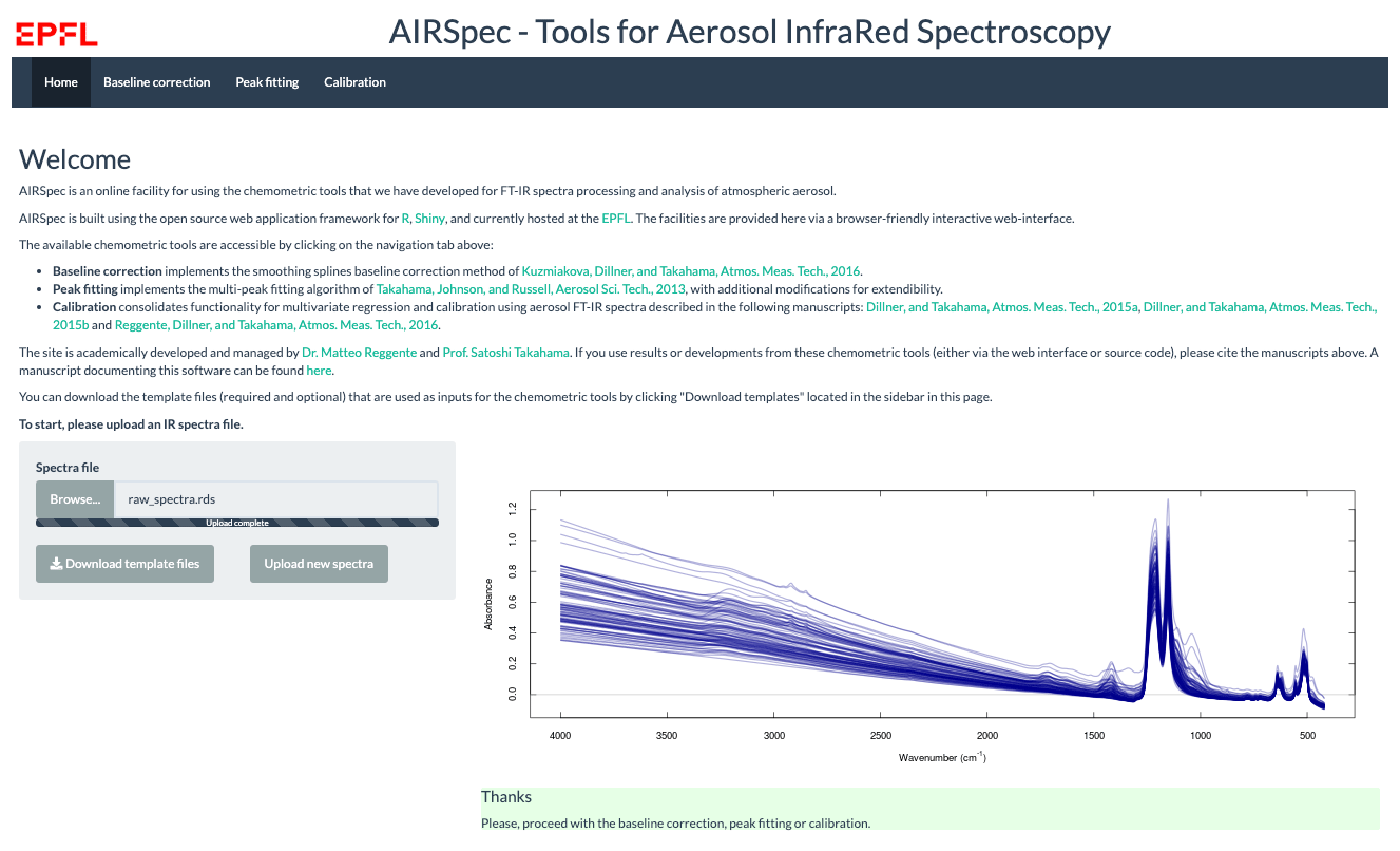
Figure 2 AIRSpec home page.

Table 1 List of inputs for each chemometric package.

2.2.1 Home page

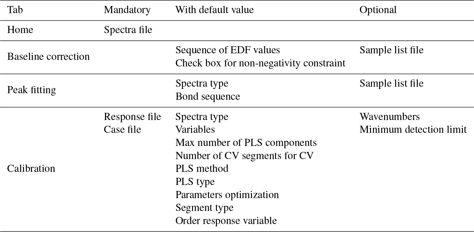
On this home page, the user typically uploads the spectra file, after which 100 random spectra are plotted for confirmation (Fig. 2). The user can then access the available chemometric packages through the additional navigation tabs. Each tab corresponds to a chemometric package, and the user can upload required and optional files or change default inputs (Table 1 summarizes the list of inputs for each tab). In each package tab, after the computation has concluded, the download button appears, and the user can retrieve an archive (zip) file containing results and input parameter files. This folder contains all the information about the analysis.

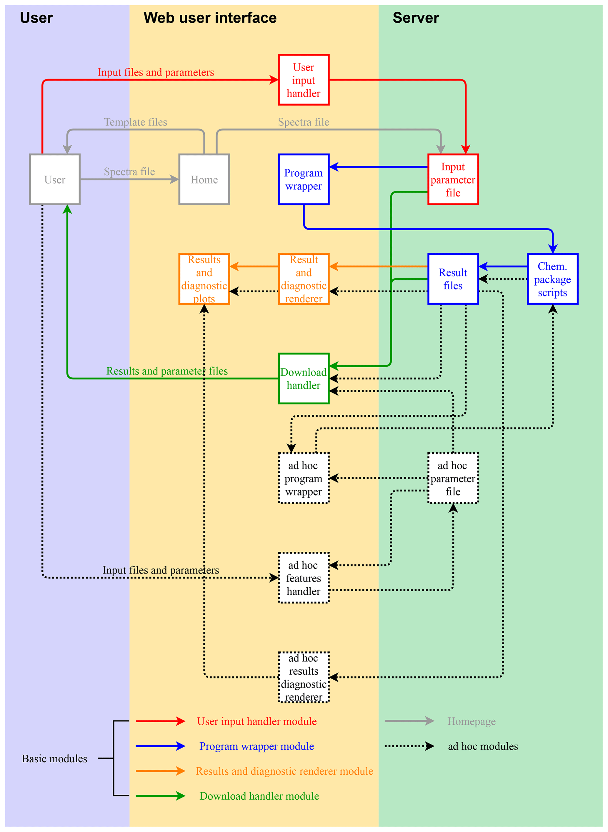
Figure 3 Chemometric package diagram and workflow. Solid boxes and arrows refer to Shiny modules used by each chemometric package (necessary modules). Supplementary features are handled by ad hoc modules and denoted by dotted boxes and arrows.

2.2.2 Tabs

In its most straightforward configuration, a chemometric package deployed on AIRSpec (solid boxes and arrows in Fig. 3) requires a script which accepts an input parameter file (JSON format) and four nested Shiny modules, which are described in turn. The user input handler module (solid red lines) writes the user inputs to the input parameter file stored in the server. The program wrapper (solid blue lines) runs the scripts of the chemometric package, passing the location of the input parameter file and saving the output files in the same folder of the input parameter file. The results and diagnostic renderer (solid orange lines) plot the output. Finally, the download handler (solid green lines) prepares and archives the input parameter file and source code output in a downloadable file.

Except for the specifications of the user input handler (e.g., input files, parameters), all the modules are general and used by each chemometric package. Therefore, to incorporate functionalities of a new package, the user only needs to prepare the package scripts and the module containing specifications of the permitted user inputs. AIRSpec additionally uses nested modules to handle ad hoc features such as dynamic input handling or ad hoc reactive plots. Again, because of the modular structure, the addition of ad hoc features does not require the changing of the necessary modules.

2.3 Relational database integration

AIRSpec uses the APRLspec package to handle its primary data object (spectra matrix) and essential operations (e.g., selecting and merging of spectra), and I/O (input/output) functions. The primary data object defines a spectrum as a row matrix with wavenumber attributes, which is a standard data structure for multivariate analysis. A new class for this type of data is defined so that operations can manipulate spectra columns and wavenumber attributes simultaneously to reduce errors of mismatched dimensions.

With an increasing number of spectra – for example in Reggente et al. (2016) the authors used thousand of spectra for their analysis – efficiency may be gained by building a spectra archive in a central, relational database. In this way, all spectra did not need to be loaded into virtual memory at once (which can be a limiting factor in analyses) but retrieved selectively from the database as necessary. The APRLspec package provides functions for accessing and storing spectra in an SQL (Structured Query Language) relational database using the similar syntax used for spectra matrices residing in virtual memory. The current implementation has been tested and used in the baseline correction package with SQLite, an embedded relational database.

3 Chemometric packages

In this section, we briefly summarize the chemometric packages developed for the analysis of atmospheric samples and currently integrated into AIRSpec: baseline correction (APRLssb R package), peak fitting (APRLmpf R package), and multivariate calibration (APRLmvr R package). For each package, we first introduce the methods and then we illustrate the analysis that the user can obtain using AIRSpec. The results are based on aerosols samples collected on PM_2.5 Teflon filters. The samples were collected at IMPROVE sites on every third day in 2011. The sample collection methods and results have been already discussed in previous works (Kuzmiakova et al., 2016; Takahama et al., 2016; Takahama and Ruggeri, 2017; Dillner and Takahama, 2015a, b; Reggente et al., 2016, 2019), and here we present some of the already published results, to give an example of what an AIRSpec user can obtain from it.

In the baseline package (Sect. 3.1.2), we first baseline-correct the spectra matrix, discussing the effective degrees of freedom (EDF) parameters selection. In Sect. 3.2.2, we use the baseline-corrected spectra of two samples (one collected at the urban site Phoenix, Arizona, and one collected at the rural location St. Marks, Florida) to quantify the FGs, the organic matter (OM), and the ratio between OM and organic carbon (OC, OM∕OC). In Sect. 3.3.2, we use the baseline-corrected spectra and collocated measurements of OC and elemental carbon (EC) – measured with thermal–optical methods – to calibrate the spectra to estimate unseen OC and EC concentrations.

3.1 Smoothing spline baseline correction

3.1.1 Background

Instrumental drift and scattering by particles and substrate used for their collection create interfering signals that hinder quantitative analysis. For the transmission mode spectra of particles collected onto PTFE presented here (obtained by ratioing sample to background single beam spectra), the subtraction of the spectrum filter before sample exposure (blank) from the aerosol spectrum has been shown to provide an insufficient remedy (Takahama et al., 2013). A smoothing spline (Reinsch, 1967) is used to model the baseline by regressing onto background regions (where no analyte absorption is expected) and interpolating through the analyte region (Kuzmiakova et al., 2016). The spectrum is divided into multiple regions so that optimal baseline correction parameters can be obtained for each segment. For each spectrum and each segment, the baseline is obtained for a given smoothness penalty λ by minimizing the objective function

$$\begin{array}{}\text{(1)}& {\displaystyle }{\displaystyle }{\min }_{\widehat{f}}\sum _{j=\mathrm{1}}^N{w}_j{\left[y_j-\widehat{f}\left({\stackrel{\mathrm{̃}}{\mathit{\nu }}}_j\right)\right]}^{\mathrm{2}}+\mathit{\lambda }\int \left[{\widehat{f}}^{\prime \prime }\right(t){]}^{\mathrm{2}}\mathrm{d}t.\end{array}$$

y_j and $\widehat{f}\left({\stackrel{\mathrm{̃}}{\mathit{\nu }}}_j\right)$ are observed and fitted absorbances at wavenumber j, respectively, and λ is a smoothing penalty. The first term represents the fidelity of fitted values to the background absorbance, and the regularization term imposes rigidity on $\widehat{f}\left({\stackrel{\mathrm{̃}}{\mathit{\nu }}}_j\right)$. The baseline is approximated by a natural cubic spline basis $\widehat{f}\left(\stackrel{\mathrm{̃}}{\mathit{\nu }}\right)=\sum _{i=\mathrm{1}}^N{B}_i\left(\stackrel{\mathrm{̃}}{\mathit{\nu }}\right){\mathit{\alpha }}_i$ with coefficient α for each basis function. w is the weight at wavenumber j, which we define as

$$\begin{array}{}\text{(2)}& {\displaystyle }{\displaystyle }{w}_j=\left\{\begin{array}{ccl}\mathrm{0}& \mathrm{if}& {\stackrel{\mathrm{̃}}{\mathit{\nu }}}_j\in {\mathcal{W}}_A\left(\mathrm{analyte}\mathrm{region}\right)\\ \mathrm{1}& \mathrm{if}& {\stackrel{\mathrm{̃}}{\mathit{\nu }}}_j\in {\mathcal{W}}_B\left(\mathrm{background}\mathrm{region}\right)\end{array}\right..\end{array}$$

λ has a monotonic relationship with the EDF of the smoothing spline fit (Hastie and Tibshirani, 1990; Green and Silverman, 1993), for which candidate values can be more easily understood through analogy to that of projection matrices commonly used in regression more generally. Letting $\mathit{f}=\left[f\right({\stackrel{\mathrm{̃}}{\mathit{\nu }}}_j\left)\right]$, W=diag(w_j), ${\mathbf{\Omega }}_N=[\int B_i^{\prime \prime }(t\left)B_j^{\prime \prime }\right(t\left)\mathrm{d}t\right]$, and $\mathbf{K}=({\mathbf{B}}^T{)}^{-\mathrm{1}}{\mathbf{\Omega }}_N{\mathbf{B}}^{-\mathrm{1}}$ with $\mathbf{B}=\left[B_i\right({\stackrel{\mathrm{̃}}{\mathit{\nu }}}_j\left)\right]$, Eq. (1) can be written as

$${\displaystyle }{\displaystyle }{\min }_{\widehat{\mathit{f}}}(\mathit{y}-\mathit{f}{)}^T\mathbf{W}(\mathit{y}-\mathit{f})+\mathit{\lambda }{\mathit{f}}^T\mathbf{K}\mathit{f},$$

for which the solution is given as a transformed version of the original spectrum:

$$\begin{array}{ll}{\displaystyle }\widehat{\mathit{f}}=\mathbf{B}\widehat{\mathit{\alpha }}& {\displaystyle }=\mathbf{B}{\left({\mathbf{B}}^T\mathbf{WB}+\mathit{\lambda }{\mathbf{\Omega }}_N\right)}^{-\mathrm{1}}{\mathbf{B}}^T\mathbf{W}\mathit{y}\\ \text{(3)}& {\displaystyle }& {\displaystyle }={\left(\mathbf{W}+\mathit{\lambda }\mathbf{K}\right)}^{-\mathrm{1}}\mathbf{W}\mathit{y}={\mathbf{S}}_{\mathit{\lambda }}\mathit{y}.\end{array}$$

For a given value of λ, the corresponding EDF_λ=Tr(S_λ) is defined by the trace of the smoother matrix S_λ, which in turn depends on the penalty matrix K and the regression weights W (Eq. 3). EDF replaces λ and its value effectively determines the rigidness of the resulting baseline (EDF = 2 is a straight line) and must be selected by the user. For a candidate set of EDF values, the negative absorbance fraction (NAF) is used to evaluate whether a physically realistic spectrum is obtained. NAF represents the contribution of negative analyte absorbance, $\left|\right|{\mathit{a}}_{A-}|{|}_{\mathrm{1}}$, to the total analyte absorbance, $\left|\right|{\mathit{a}}_A|{|}_{\mathrm{1}}$:

$$\begin{array}{}\text{(4)}& {\displaystyle }{\displaystyle }\mathrm{NAF}={\displaystyle \frac{\left|\right|{\mathit{a}}_{A-}|{|}_{\mathrm{1}}}{\left|\right|{\mathit{a}}_A|{|}_{\mathrm{1}}}}\times \mathrm{100}\mathit{\%},\end{array}$$

where $\left|\right|\cdot |{|}_{\mathrm{1}}$ denotes the 1-norm magnitude of a vector (summation of all absolute values of vector elements). NAF is calculated across the entire wavenumber range in the analyte region of in a given segment.

In our current implementation, we provide 𝒲_B for two segments (4000–1820 and 2000–1500 cm⁻¹) in the high-frequency region (>1500 cm⁻¹) of the spectrum where stretching and bending modes of bonds in carbon–hydrogen, carboxylic acid, carbonyl, hydroxyl, and primary amine groups are present (Maria et al., 2003a). This region has been used extensively for functional group analysis (Russell et al., 2011; Takahama et al., 2013) and estimation of carbon content (Dillner and Takahama, 2015a, b). The values of 𝒲_B provided undergo iterative adjustment by the algorithm to further avoid negative regions, and with this approach have generated suitable baselines for ambient PM samples (Kuzmiakova et al., 2016). However, use with laboratory samples with specific absorption patterns and low concentrations may require additional adjustment.

3.1.2 Implementation

Browser interface

In the baseline correction tab, the user can upload an optional file containing the list of samples to process; AIRSpec will otherwise baseline-correct all the samples present in the uploaded spectra file. A sequence of EDF values for which different baselines are computed and compared is provided by default but can be edited by the user. When interpolating over a wide region with substantial curvature, negative regions may arise for any EDF if the degree of curvature is not well captured by the pre-specified background regions. AIRSpec provides an option to impose a non-negativity constraint, in which interior points with substantially negative values are iteratively added to 𝒲_B during the fitting process. This heuristic approach provides a lower-bound envelope of the actual absorbance that is discernable from the spectrum. By clicking the Compute button, AIRSpec will execute prepared scripts, passing as input a file with the desired configuration generated from user choices. At the end of the computation, AIRSpec plots the spectra of the baseline-corrected samples using the EDF parameter, which minimizes the median of the NAF (Kuzmiakova et al., 2016). The EDF value can be changed by the user a posteriori, after which the plot will automatically update. 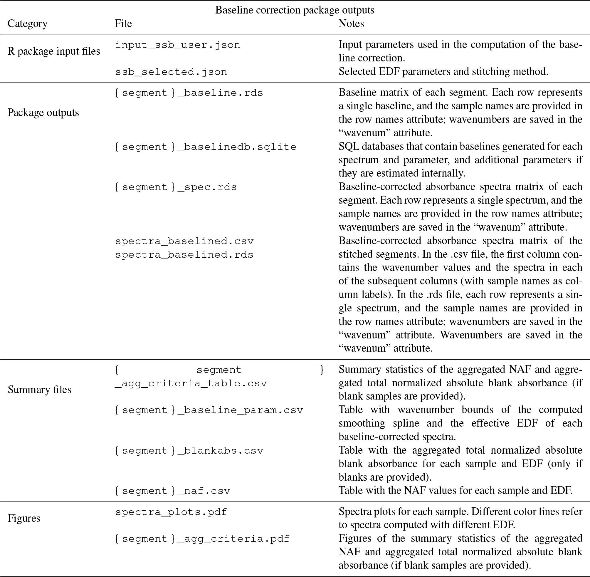A list of the output files can be found in Table 2 and in the dedicated wiki tab in the web interface.

Example output

Figure 4a shows the unprocessed and the baseline-corrected spectra of ambient samples collected on PTFE filters. The scatter from PTFE fibers results in a sloping baseline that masks the absorbance bands and therefore makes it challenging to extract the analyte contributions (unprocessed spectra). Moreover, the baseline is not the same for each spectrum on account of fiber orientation and stretching. These variances make standardized baseline preprocessing methods (e.g., blanks spectra or pre-scan subtraction) insufficient – a detailed description of these ambient samples can be found in the companion paper (Reggente et al., 2019).

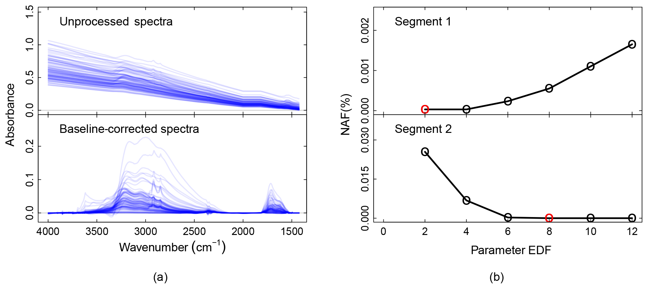
Figure 4 Baseline correction package outputs. (a) From top to down, the panels show the unprocessed and the baseline-corrected spectra of ambient samples collected on PTFE filters. A detailed description of these ambient samples can be found in the companion paper (Reggente et al., 2019). Absorbance scale in arbitrary units (a.u.). (b) The EDF selection criteria for segment one and two. The red circles represent the EDF values that minimize the median of the selection criteria NAF. In the current implementation of the chemometric package, segment one and two refer to spectra in the regions 4000–1820 and 2000–1500 cm⁻¹, respectively (Kuzmiakova et al., 2016).

In the baseline-corrected spectra (Fig. 4a) the features due to the analyte are more evident than the previous case. For example, the aNH₂ and CO peaks (around 1600 and 1700 cm⁻¹ respectively) are easily distinguishable, and it is possible to notice that there are filters with different amounts of these two FGs. Similarly, the sharp peaks around 2800 and 2900 cm⁻¹ are due to the presence of aCH, and the two broad peaks around 3100 and 3300 cm⁻¹ are due to the presence of ammonium (ammNH), aCOH, COOH, and to lesser extent to aromatic CH and alkene CH.

Table 2 List of outputs of the baseline correction chemometric package. {segment} denotes the segment label.

The baseline-corrected spectra have been computed using the EDF values that minimize the median of the NAF metric. We computed the baseline for different EDF values (2, 4, 6, 8, 10, 12 – the user can change these values), and the EDF values selected are 2 and 8 for segment 1 and 2 respectively (red dots in Fig. 4b). The AIRSpec user can check these diagnostic plots in the parameter selection tab and change the proposed EDF values using the input field provided in the web interface. Moreover, the user, using the implemented interactive plot, can immediately see the changes in the spectrum shapes when changing the EDF parameters, thus facilitating the exploratory work and parameter selection task.

3.2 Peak fitting

3.2.1 Background

The peak-fitting package implements a physically based approach to FG quantification (Alsberg et al., 1997). This method decomposes each spectrum in Gaussian peaks or line shapes which represent the absorption profile of individual bonds. The FG abundances are estimated by relating absorption peaks or line shapes with their molar absorption coefficients as described by Takahama et al. (2013).

The analysis consists of three parts: (i) estimation of molar abundances of bonds from peak areas, (ii) reapportionment of bonds to functional groups, (iii) estimation of atomic abundances from functional group abundances (from which OM, OM∕OC, O∕C are derived). In the following equations, s denotes a line-shape function defined over wavenumbers ${\stackrel{\mathrm{̃}}{\mathit{\nu }}}_{j}s$ and a set of peak parameters θ_ik for sample i for bond k. The integrated absorbance (peak area), together with a molar absorption coefficient and for the bond, is used to estimate the number of moles of bond per unit area of sample (denoted by n):

$$\begin{array}{}\text{(5)}& {\displaystyle }& {\displaystyle }{n}_{ik}={\stackrel{\mathrm{‾}}{\mathit{\epsilon }}}_k\mathrm{\Delta }\stackrel{\mathrm{̃}}{\mathit{\nu }}\sum _j{q}_{j}s\left({\stackrel{\mathrm{̃}}{\mathit{\nu }}}_j,{\mathit{\theta }}_{ik}\right)\text{(6)}& {\displaystyle }& {\displaystyle }{x}_{ij}=\sum _{k}s\left({\stackrel{\mathrm{̃}}{\mathit{\nu }}}_j,{\mathit{\theta }}_{ik}\right)+e_{ij}.\end{array}$$

q_js denotes quadrature coefficients for numerical integration. For a Gaussian line shape, θ_ik may correspond to any number of relevant amplitude, location, and width parameters for each bond, and an analytical solution exists for its integral. For fixed line shapes (e.g., cCOH), the peak parameter corresponds to a scaling coefficient. Current default values for molar absorption coefficients ε_k are those reported by Russell et al. (2009a) and Takahama et al. (2013).

The total carbonyl (tCO) quantified by peak fitting can include contributions from carboxyl, ketone, ester, and aldehyde carbonyl because of their proximity in absorption bands that are difficult to resolve in environmental samples (Takahama et al., 2013; Reggente et al., 2019). Therefore, we apportion tCO to acid (COOH) and non-acid CO (naCO):

$$\begin{array}{ll}{\displaystyle }& {\displaystyle }\left(n_{\mathrm{COOH}},n_{\mathrm{naCO}}\right)=\\ \text{(7)}& {\displaystyle }& {\displaystyle }\left\{\begin{array}{ll}\left(n_{\mathrm{COOH}},n_{\mathrm{tCO}}-n_{\mathrm{COOH}}\right),& \mathrm{if}{n}_{\mathrm{tCO}}>n_{\mathrm{COOH}}\\ \left(n_{\mathrm{COOH}},\mathrm{0}\right),& \mathrm{otherwise}\end{array}\right..\end{array}$$

Using this convention, we estimate apportionment on an individual sample basis rather than in aggregate as described by Takahama et al. (2013). We compute the OC mass, OM∕OC ratios, and O∕C ratios by the constituent atomic molar abundance n_a, which is calculated from moles n_k for FG k through a coefficient λ_ak such that n_a=λ_akn_k. The values of λ_ak are set according to the bonding configuration proposed by Takahama and Ruggeri (2017).

$$\begin{array}{}\text{(8)}& {\displaystyle }{\displaystyle }\left(\begin{array}{c}{n}_{\mathrm{C}}\\ n_{\mathrm{O}}\\ n_{\mathrm{H}}\end{array}\right)=\left(\begin{array}{ccccc}\mathrm{0.5}& \mathrm{1}& \mathrm{0.5}& \mathrm{1}& \mathrm{0.25}\\ \mathrm{1}& \mathrm{2}& \mathrm{0}& \mathrm{1}& \mathrm{0}\\ \mathrm{1}& \mathrm{1}& \mathrm{1}& \mathrm{0}& \mathrm{1}\end{array}\right)\left(\begin{array}{c}{n}_{\mathrm{aCOH}}\\ n_{\mathrm{COOH}}\\ n_{\mathrm{aCH}}\\ n_{\mathrm{naCO}}\\ n_{\mathrm{NH}}\end{array}\right).\end{array}$$

In contrast to previous studies (Russell, 2003; Ruthenburg et al., 2014), Takahama and Ruggeri (2017) proposed the value of 0.5 for λ_C⋅aCOH, which is consistent with past work by Russell et al. (2009b). A value of 0.5 corresponds to the assumption that the carbon shares an aCOH bond with a single aCH bond, whereas a value of 0 corresponds to the assumption of a terminal saturated carbon in which it is accounted for by two aCH bonds. A more detailed discussion of FG quantification in atmospheric aerosol samples by FTIR is provided in the companion paper of this work (Reggente et al., 2019).

3.2.2 Implementation

Browser interface

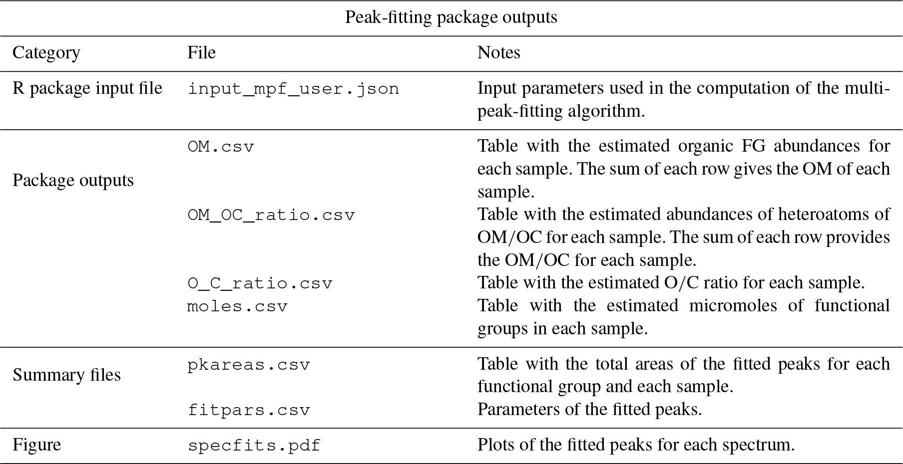
In the peak-fitting tab, the user can choose to use the uploaded spectra matrix file (uploaded in home tab) or, if already computed, the baseline-corrected spectra matrix (output of the baseline correction tab). Moreover, the user can choose the sequence of FGs (default provided) to be fitted, and the samples to process (as default AIRSpec will peak-fit all the samples present in the spectra matrix). By clicking the Compute button, AIRSpec will execute prepared scripts, passing as input a file with the desired configuration. At the end of the computation, AIRSpec plots each spectrum with the fitted peaks. Moreover, the user can download a table containing the FG distribution in organic mass (OM) and the OM∕OC ratio (for each sample). A list of the available files can be found in Table 3 and in the dedicated wiki tab in the web interface.

Example output

We fit individual Gaussian line shapes to obtain the abundance (in moles) of aCOH, COOH, aCH, CO, and aNH₂ from the baseline-corrected spectra. Figure 5a shows the fitted peaks and the spectra of the sample collected at one rural and one urban site. According to the Beer–Lambert law (variations of FGs abundance are linearly dependent to the absorbance), from a visual comparison of the two samples, we can note that the urban sample is characterized by greater abundance of aNH₂ (orange peaks around 1600 cm⁻¹) and CO (dark green peaks around 1700 cm⁻¹) FGs. Moreover, the urban sample shows greater abundances of COOH (light green bimodal line) and aCH (sharps blue peaks around 2800 and 2900 cm⁻¹). The rural site, instead, is characterized by a greater abundance of ammNH (dark orange bimodal line).

AIRSpec provides FG abundance in several representations: the areal density (µmole cm⁻²) calculated from Eq. (4), the areal mass density (µg cm⁻²) obtained from Eq. (4), and the atomic masses of each element. The OM (in units of µg cm⁻²) summed from FG contributions is also provided. To obtain atmospheric concentrations (µg m⁻³), it is necessary to multiply these areal mass densities by the substrate collection area and divide by the volume of air sampled (3.53 cm² and 32.8 m³, respectively, for examples shown in this article). In Fig. 5b, the first bar plot compares the FG distribution in the OM for the two samples. First, we note that OM is higher at the urban site, and the aCH accounts the 38 % and 57 % of the total OM at the rural and urban site respectively. These differences are mainly due to the higher impact of anthropogenic sources at the urban site. Moreover the significant contributions of aCOH (21 % and 14 % in the rural and urban samples respectively) and COOH (34 % and 23 % respectively) exemplify the influence of processed aerosol from surrounding regions affecting the PM_2.5.

Moreover, the OM∕OC and O∕C ratios (second and third bar plots in Fig. 5b respectively) are higher at the rural site than the urban (2.08 and 1.72 respectively). This result is in agreement with measurements by GC-MS and AMS (Turpin and Lim, 2001; Aiken et al., 2008) and can be explained by the condensation of functionalized molecules (Ziemann, 2005; Kroll and Seinfeld, 2008) and heterogeneous reactions (Smith et al., 2009; Lim et al., 2010) which lead to chemical aging.

Figure 5 Peak-fitting package outputs. Example of FG analysis by FT-IR spectroscopy of atmospheric aerosol collected on one Teflon filter. (a) Baseline-corrected spectra (black lines) with fitted FGs (colored lines) for the rural (top panel) and urban (bottom panel) samples. (b) From left to right the bar plots represent the FG contributions to total OM, their non-carbon contributions to the total OM∕OC ratio (Takahama and Ruggeri, 2017), and the O∕C atomic ratio for rural and urban samples.

Table 3 List of outputs of the peak-fitting chemometric package.

3.3 Multivariate calibration

3.3.1 Background

Multivariate calibration is a general technique that can be applied for prediction of functional groups or any arbitrary property to which spectra can be related. Many decisions for this implementation are based on the work of Dillner and Takahama (2015a, b) to predict carbonaceous content and EC from FTIR spectra. The calibration package uses partial least squares regression (PLSR, Wold et al., 1983b; Geladi and Kowalski, 1986) implemented by the PLS package (Mevik and Wehrens, 2007) of the R statistical environment (R Core Team, 2016). The goal is to estimate a set of coefficients B from a matrix of mean-centered spectra X for mean-centered response variables Y, with residuals E:

$$\begin{array}{}\text{(9)}& {\displaystyle }{\displaystyle }\mathbf{Y}=\mathbf{XB}+\mathbf{E}.\end{array}$$

Because strong correlation of absorbances across wavenumbers (collinearity) exists among variables in X and the number of wavenumbers in X exceeds the number of observations, PLSR is used to combine correlated features into a smaller number of latent variables. PLSR performs a bilinear decomposition of both X and Y: X is decomposed into a product of orthogonal factors (X loadings, P) and their respective contributions (scores, T), while Y is decomposed reconstructed through T and their coefficients (or Y loadings, Q):

$$\begin{array}{}\text{(10)}& {\displaystyle }& {\displaystyle }\mathbf{X}={\mathbf{TP}}^T+\mathbf{F}\text{(11)}& {\displaystyle }& {\displaystyle }\mathbf{Y}={\mathbf{TQ}}^T+\mathbf{E}.\end{array}$$

T captures the variations across both X and Y. B can be estimated from a matrix of direction vectors $\mathbf{R}=\mathbf{W}({\mathbf{P}}^T\mathbf{W}{)}^{-\mathrm{1}}$ found to maximize covariance of transformed X with Y (hats over symbols denote statistically estimated quantities):

$$\begin{array}{ll}{\displaystyle }& {\displaystyle }\widehat{\mathbf{T}}=\mathbf{X}\widehat{\mathbf{R}}\\ {\displaystyle }& {\displaystyle }\widehat{\mathbf{B}}=\widehat{\mathbf{R}}{\widehat{\mathbf{Q}}}^T.\end{array}$$

Candidate models for calibration are generated by varying the number of factors (or latent variables LVs) used to represent the matrix of spectra. The anticipated performance of the model for each number of factors is estimated using root mean square error of cross-validation (CV) (Hastie et al., 2009; Arlot and Celisse, 2010), and by default the model with the minimum value is selected.

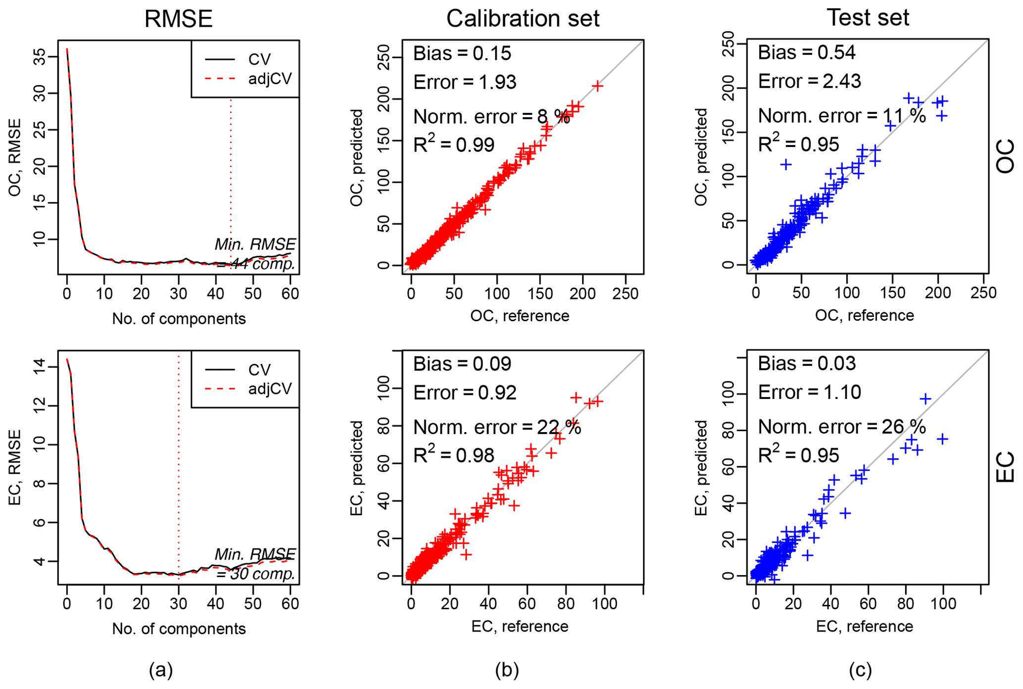
Figure 6 Calibration package. Example of calibration output. (a) RMSE in cross-validation against the number of components (latent variables), and the dotted vertical line indicates the number of components selected according to the minimum RMSE. (b) and (c) indicate scatterplots of predicted against observed (or reference) values for the calibration and test datasets respectively.

Further measures for model interpretation are provided. The explained variation in the response variable, EV${}_{\mathrm{r}k}^{\left(Y\right)}$, varies between 0 and 1 and describes the contribution of component k to the variance of the response variable r. The explained variation in the spectra, EV${}_{jk}^{\left(X\right)}$, varies between 0 and 1 describes the contribution of component k to the variance of the spectra at wavenumber j. The variable importance in projection (VIP) (Wold et al., 1983a) provides complementary information to EV${}_{jk}^{\left(X\right)}$ in that it assesses the weighting of the jth wavenumber toward the explained variation in the response variable. VIP scores greater than unity for any wavenumber suggests their importance, but this value can in practice vary according to the noise level and the number of uninformative variables (Chong and Jun, 2005a). These expressions are calculated from the measurement and model sum of squares:

$$\begin{array}{ll}{\displaystyle }& {\displaystyle }{\mathrm{EV}}_{\mathrm{r}k}^{\left(Y\right)}={\displaystyle \frac{\mathrm{Tr}\left({\mathbf{T}}^T\mathbf{T}\right)\cdot \mathrm{Tr}\left({\mathbf{QQ}}^T\right)}{\mathrm{Tr}\left({\mathbf{Y}}^T\mathbf{Y}\right)}}={\displaystyle \frac{\left({\mathit{t}}_k^T{\mathit{t}}_k\right)\cdot \left({\mathit{q}}_{\mathrm{r}}^T{\mathit{q}}_{\mathrm{r}}\right)}{{\mathbf{y}}_{\mathrm{r}}^T{\mathbf{y}}_{\mathrm{r}}}}\\ {\displaystyle }& {\displaystyle }{\mathrm{EV}}_{jk}^{\left(X\right)}={\displaystyle \frac{\mathrm{Tr}\left({\mathbf{T}}^T\mathbf{T}\right)\cdot \mathrm{Tr}\left({\mathbf{PP}}^T\right)}{\mathrm{Tr}\left({\mathbf{X}}^T\mathbf{X}\right)}}={\displaystyle \frac{\left({\mathit{t}}_k^T{\mathit{t}}_k\right)\cdot \left({\mathit{p}}_j^T{\mathit{p}}_j\right)}{{\mathit{x}}_j^T{\mathit{x}}_j}}\\ {\displaystyle }& {\displaystyle }{\mathrm{VIP}}_{\mathrm{r}jk}={\left(N{\displaystyle \frac{\sum _{\mathrm{\ell }=\mathrm{1}}^k{\mathrm{EV}}_{\mathrm{r}\mathrm{\ell }}^{\left(Y\right)}{w}_{j\mathrm{\ell }}^{\mathrm{2}}}{\sum _{\mathrm{\ell }=\mathrm{1}}^k{\mathrm{EV}}_{\mathrm{r}\mathrm{\ell }}^{\left(Y\right)}}}\right)}^{\mathrm{1}/\mathrm{2}}.\end{array}$$

N is the number of wavenumbers, and w is the elements of unit normal weight vectors, which together with X loadings construct the direction vectors R. Tr(⋅) is the trace of the matrix. Their use is described by our companion paper (Reggente et al., 2019).

3.3.2 Implementation

Browser interface

In the calibration tab, the user can choose to use the uploaded spectra matrix file (uploaded in home tab) or, if already computed, the baseline-corrected spectra matrix (output of the baseline correction tab). Two additional files are required: one containing the response values (target variables), and one containing the list of samples to be used for calibration and test. After providing the response file, the user chooses the target variables of the regression from a list given by the column names of the response file uploaded. The user can choose single or multiple variables, and accordingly to the type of PLS desired (PLS type field). In the case of multiple variables, AIRSpec will process a regression model for each variable (PLS1) or a regression model for the whole matrix of variables (PLS2). The user can also upload an optional file to use only specified wavenumbers or to exclude responses below the minimum detection limit of the response variable. Moreover, the user can change the default parameters used in the regression (e.g., fitting algorithm, parameters optimization criteria, limit the number of latent variables). By clicking the Compute button, AIRSpec will execute prepared scripts, passing as input a file with the desired configuration. Evaluation of models by RMSE of cross-validation, detailed statistics (figures of merit) of the calibration models, prediction values, and the diagnostic measures (EVs and VIP) are provided. A list of the available files can be found in Table 4 and in the dedicated wiki tab in the web interface.

Example output

We present an example of organic and elemental carbon (OC and EC, respectively) prediction analyzed by thermal optical reflectance (TOR). Dillner and Takahama (2015a, b) demonstrated that the FTIR spectra of aerosol samples collected on Teflon filters could be used to estimate OC and EC concentrations by building a calibration model using FTIR spectra paired with collocated quartz fiber filters analyzed for TOR OC and EC. These models achieved accuracy and precision on a par with the TOR precision for samples collected in the same year and at the same sites as those included in the calibration. Reggente et al. (2016) showed that the same calibration model could be used in different years and at different sites when concentration range and composition of carbonaceous samples in the calibration set approximately resemble those in the prediction set (new samples for which predictions are desired).

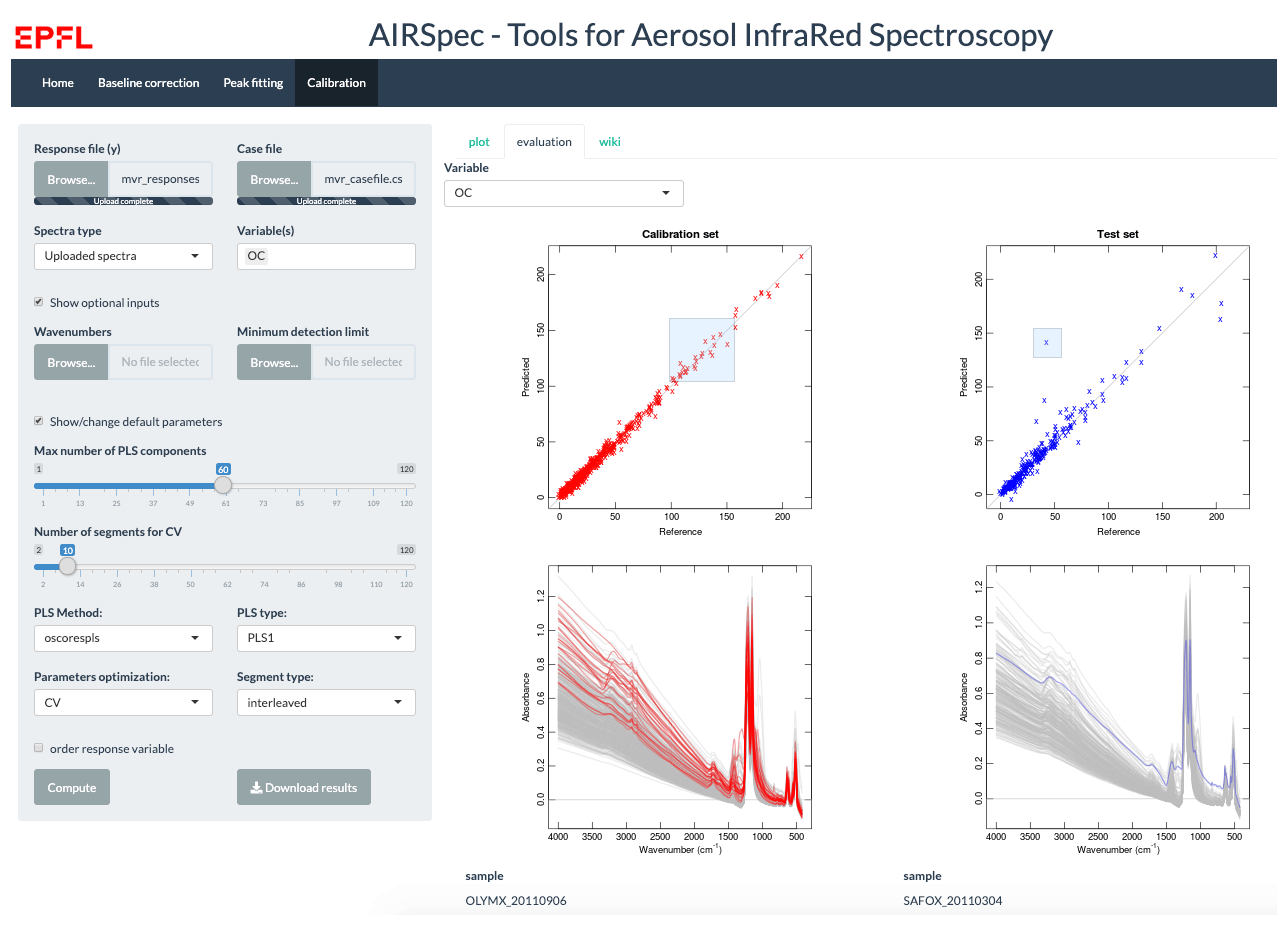
Figure 7 AIRSpec calibration package tab.

Chong and Jun (2005b)

Table 4 List of outputs of the calibration chemometric package.

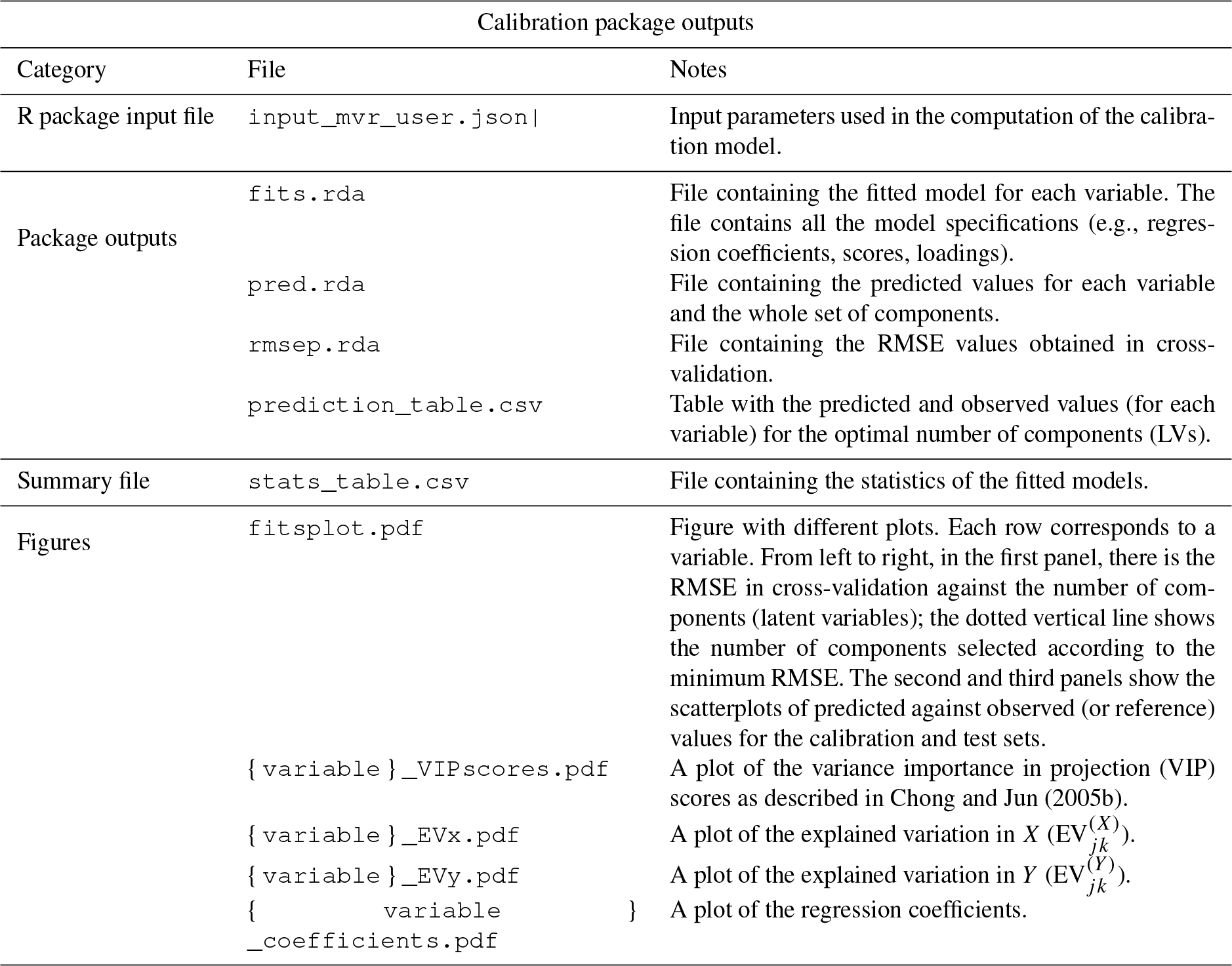
Figure 6 shows the results of the calibration models for OC (top row) and EC (bottom row); 794 IMPROVE samples and 54 blanks are divided into two sets: one is used for model training and parameter selection (calibration set), and one is used for the evaluation (test set). The calibration set contains two-thirds of the total (chronologically stratified within each site) and the test set the remaining third. We used the baseline-corrected spectra (output of the baseline correction package, Sect. 3.1.2).

The first column of Fig. 6a shows the RMSE in cross-validation against the number of components (latent variables), and the dotted vertical line indicates the number of components selected according to the minimum RMSE. The second and third columns show the scatterplots of predicted against observed (or reference) values for the calibration (b) and test datasets (c) respectively. Bias (median difference between measured and predicted), error (median absolute bias), normalized error (median of the error divided by each measured value), and the coefficient of determination of the linear regression fit of the predicted and measured values (R²) are reported in each scatterplot. The scatterplots and metrics revealed that there is a good agreement between measured (OC and EC reference) and predicted OC and EC values. A detailed description and discussion of these results are described by Dillner and Takahama (2015a, b). In the evaluation tab (Fig. 7), there are interactive plots to highlight the desired spectra. The user can select samples from the scatterplots (using a brush tool, square boxes in Fig. 7), and then the selected spectra will change color (red for calibration samples and blue for test samples). This plot can help the user in interpreting the prediction performances, by, for example, comparing the spectra of samples with different prediction quality.

4 Summary and future development

FTIR spectroscopy is a useful tool for obtaining the functional group representation of the chemical composition of atmospheric PM. However, the complexity of FTIR spectra of PM requires algorithms for consistent interpretation applied across diverse samples. AIRSpec provides a framework for centralizing and disseminating such algorithms. We present three examples of packages implemented for specific tasks: baseline correction, peak fitting, and multivariate calibration. The decoupling of the user interface with the bulk of underlying computation provides flexibility in that exploratory work can be performed with the former, while batch computations can be carried out directly through shell scripts and new scripts can be written to take advantage of existing functions in the underlying packages. The browser interface generates input files so that provenance between input parameters and computation results are preserved, and users can use input files as templates for new computations. The outputs of the program include diagnostic plots, tables of calculations, and statistics that are relevant to the atmospheric aerosol analysis. The modular architecture exploits common patterns in input specification, computation, and user interaction such that implementation of new collections of algorithms is facilitated by reuse of existing functions. Incorporation of factor and cluster analyses, sparse calibration, and other algorithms is anticipated for future development.