A method to assess the accuracy of sonic anemometer measurements

We propose a method to assess the accuracy of atmospheric turbulence measurements performed by sonic anemometers and test it by analysis of measurements from two commonly used sonic anemometers, a Metek USA-1 and a Campbell CSAT3, at two locations in Denmark. The method relies on the estimation of the ratio of the vertical to the along-wind velocity power spectrum within the inertial subrange and does not require the use of another measurement as reference. When we correct the USA-1 to account for three-dimensional flow-distortion effects, as recommended by Metek GmbH, the ratio is very close to 4∕3 as expected from Kolmogorov's hypothesis, whereas non-corrected data show a ratio close to 1. For the CSAT3, non-corrected data show a ratio close to 1.1 for the two sites and for wind directions where the instrument is not directly affected by the mast. After applying a previously suggested flow-distortion correction, the ratio increases up to ≈1.2, implying that the effect of flow distortion in this instrument is still not properly accounted for.

1 Introduction

Accurate observations of atmospheric flow velocities, turbulence, and turbulence fluxes are critical for our understanding of all physical processes that occur in the atmospheric boundary layer and for the improvement of atmospheric modeling. Examples of intensely researched applications of turbulent fluxes include the closure of the surface energy balance (Foken, 2008), as well as the estimation of the carbon balance based on eddy-covariance observations, in which a very small systematic error can have a significant effect on the yearly carbon budget (Ibrom et al., 2007). Other applications include wind-power meteorology: turbulence is an important design parameter for wind turbines as the turbine loads are directly related to the velocity variances, and turbulence measurements are therefore needed to find out whether a wind turbine can withstand the local flow conditions (Dimitrov et al., 2015; Mücke et al., 2011).

Our current understanding of atmospheric turbulence is, to a high degree, based on measurements performed with three-dimensional sonic anemometers deployed on meteorological towers. However, sonic anemometer measurements suffer from flow distortion due to the effects of both the structure(s) where the anemometer is mounted on, i.e., booms, clamps, and the bulk of the mast itself (Dyer, 1981; McCaffrey et al., 2017), and the anemometer itself. The latter effect has been recognized as a limitation for the accuracy of sonic anemometer observations for several decades (Grelle and Lindroth, 1994; Horst et al., 2015; Wyngaard, 1981; Zhang et al., 1986; van der Molen et al., 2004).

Some of the first wind-tunnel investigations on how the sonic anemometer structure impacts the measurements' accuracy were performed on the Kaijo Denki DAT-300 sonic anemometer (Kraan and Oost, 1989; Mortensen, 1994). They showed azimuth-dependent errors in the observed wind speed, which reflected the geometry of the probe head. These studies were followed by wind-tunnel investigations of the much more slender Gill R2 sonic anemometers by Grelle and Lindroth (1994), who showed the influence from the three supporting bars on the probe head leading to maximum wind speed errors of 15 %, whereas the change of tilt within a small interval of angles showed less effect. This study was followed by that of Mortensen and Højstrup (1995), who showed influence on the accuracy of the measured velocity both from the ambient temperature and wind speed. Later, van der Molen et al. (2004) investigated Gill R2 and R3 sonic anemometers for a much wider range of tilt angles than those from the previous two studies. They demonstrated that the vertical velocity was severely underestimated at large tilt angles. Whereas surface sensible heat flux observations taken over forest increased by 4 % using the calibration scheme by Grelle and Lindroth (1994), the calibration scheme by van der Molen et al. (2004) resulted in sensible heat flux increases of 15 % for a different forested site. For the USA-1 (or its more modern version the uSonic3) sonic anemometer from Metek GmbH, Hamburg, Germany, two-dimensional and three-dimensional flow-distortion corrections were provided by Metek GmbH (2004) (hereafter M04). They are based on wind-tunnel observations for a number of azimuths and tilt angles.

Högström and Smedman (2004) documented an intercomparison between hot-film anemometers and Gill Solent R2 and R3 sonic anemometers. Both types of instruments were calibrated in a wind tunnel and subsequently intercompared in full-scale experiments. Whereas the hot-film anemometers retained their precision from the calibration, that of the sonic anemometers deteriorated in the field tests. Högström and Smedman (2004) argued that this difference could be explained by the effect of atmospheric turbulence and, hence, that wind-tunnel-based calibrations may not be valid.

Another method for testing the precision and accuracy of sonic anemometers is to mount different brands closely and study the agreement between their turbulence measurements (Kochendorfer et al., 2012; Mauder et al., 2007). The challenge with this method is the difficulty to objectively determine which of the sonic anemometers measures best. Also, if agreement is found, this could be due to a similar error.

A third variant for assessing sonic anemometer performance is by comparing several of the same brand by mounting them at different tilts (Kochendorfer et al., 2012; Meyers and Heuer, 2006; Nakai and Shimoyama, 2012) and azimuths (Kaimal et al., 1990). Nakai and Shimoyama (2012) used five WindMaster sonic anemometers mounted at different angles relative to each other and deduced flow-distortion correction schemes based on the anemometers' different responses as a function of both tilt and azimuth angles. Since the geometry of the WindMaster is identical to that of the Solent R2 and R3, the resulting flow-distortion correction scheme could be compared to that of van der Molen et al. (2004). The new scheme by Nakai and Shimoyama (2012) pointed to slightly higher increases in the turbulent fluxes than that by van der Molen et al. (2004). Kochendorfer et al. (2012) used three sonic anemometers by R. M. Young, and studied the observations of the vertical wind speed over a wide range of azimuth and tilt angles. They found that for their sites, the vertical wind speed was underestimated by ≈11 %, and when applying their derived corrections, the heat fluxes increased by 9 %–13 %. Whereas this method avoids the potential problems associated with quasi-laminar wind-tunnel calibrations, the accuracy of the correction cannot be better than the accuracy of the instrument chosen as the reference. Also, it is hard to evaluate whether the somewhat “busy” setup with several sonic anemometers in a small area could lead to additional and larger flow distortions than those using a single sonic anemometer.

Several combinations of the three different methods outlined above (wind-tunnel calibration, comparison of different brands of sonic anemometers, and tilting sonic anemometers of the same brand relative to each other) have also been demonstrated. Using four CSAT3 sonic anemometers and one ATI sonic anemometer, where two of the CSAT3 instruments were rotated 90^∘, Frank et al. (2013) showed that the CSAT3 underestimated the vertical velocities, which led to an underestimation of the sensible heat flux of about 10 %. Horst et al. (2015) (hereafter H15) used a combination of all three of the methods to derive a flow-distortion correction for the CSAT3. Their correction, when applied to sensible heat flux data taken over an orchard canopy, showed a more modest effect closer to 5 %. Based on the same data as those in Frank et al. (2013), Frank et al. (2016) demonstrated the use of a Bayesian model to estimate the most likely flow-distortion correction scheme of the CSAT3 and found a 10 % increase in vertical velocities and sensible heat flux as well. Huq et al. (2017) presented a novel approach for estimating the accuracy of the CSAT3 by using numerical simulations. The results of the study pointed to flow-distortion errors of similar magnitude as those in H15. The discrepancies in the findings of the previous studies foster the debate on the magnitude of the CSAT3 flow-distortion correction. Given the key role that sonic anemometers have in the field of experimental micrometeorology, it is of great importance to find objective standards by which accuracy and precision can be evaluated.

The aim of the current study is two-fold. First we introduce a new method for evaluating sonic anemometer accuracy, and second, we evaluate the effect of flow-distortion corrections for two different sonic anemometers using this method. The two sonic anemometers are the USA-1, for which we apply the manufacturer's flow-distortion correction, which is based on wind-tunnel measurements, and the CSAT3, for which we apply the correction by H15. To our knowledge, the method, which is based on the relation between the velocity spectra within the inertial subrange, has not been used previously for diagnosing sonic anemometer accuracy.

2 Background and methods

We first start by introducing the expected relations between velocity spectra within the inertial subrange in Sect. 2.1 and later introduce the flow corrections commonly used for sonic anemometers measurements in Sect. 2.2.

2.1 Inertial subrange

The inertial subrange corresponds to the region in the atmospheric energy spectrum where energy is neither produced nor dissipated and where the transfer of energy from the energy-containing range (buoyancy- and shear-produced energy) to the dissipation range (kinetic to internal energy) is controlled by ε, which is the rate at which energy is converted to heat in the dissipation range (Kaimal and Finnigan, 1994).

Following the dimensional considerations of Kolmogorov (1941), the power spectrum of u, which is that of the along-wind component of the velocity, within the inertial subrange becomes

$$\begin{array}{}\text{(1)}& F_u\left(k_{\mathrm{1}}\right)=\mathit{\alpha }{\mathit{\epsilon }}^{\mathrm{2}/\mathrm{3}}{k}_{\mathrm{1}}^{-\mathrm{5}/\mathrm{3}},\end{array}$$

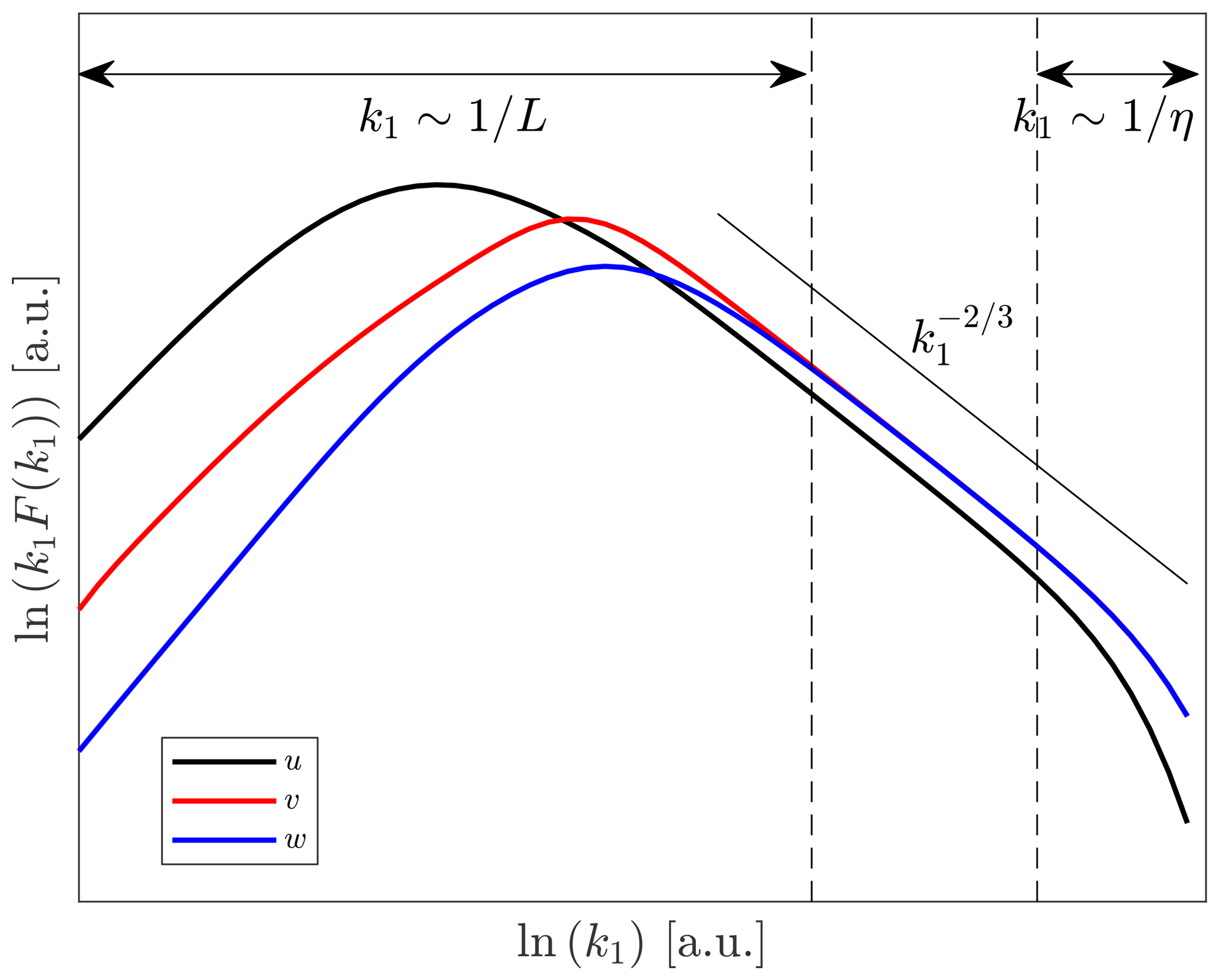
where k₁ is the along-wind wavenumber, and α is the universal Kolmogorov constant (≈0.5). Statistical isotropy of the second order means that no second-order statistics change if the coordinate system is rotated in any way. This would imply that the variances of the three velocity components would be identical and the covariances would be zero. But we can say that turbulence is locally isotropic within the inertial subrange, which means that within that range all one-point cross-spectra between different velocity components approach zero faster than the velocity-component spectra. For example, the cross-spectrum between u and w, where w is the vertical velocity component, decreases like $k_{\mathrm{1}}^{-\mathrm{7}/\mathrm{3}}$, which is more rapid than F_u and the bulk of the momentum flux $\langle u^{\prime }{w}^{\prime }\rangle$, where the prime indicates fluctuations, is located at a wavenumber lower than the inertial subrange. Due to incompressibility and isotropy, the velocity power spectra follow the relation (Pope, 2000),

$$\begin{array}{}\text{(2)}& F_w\left(k_{\mathrm{1}}\right)=F_v\left(k_{\mathrm{1}}\right)={\displaystyle \frac{\mathrm{4}}{\mathrm{3}}}{F}_u\left(k_{\mathrm{1}}\right),\end{array}$$

where v is the cross velocity component. Figure 1 illustrates idealized velocity spectra showing the spectral regions, the behavior of each velocity component, and the relations in the inertial subrange. It is important to note that Eq. (2) is only an asymptotic relation valid for $\mathrm{1}/L\ll k_{\mathrm{1}}\ll \mathrm{1}/\mathit{\eta }$ where L is an outer scale of the turbulence, for example, the most energy-containing scales, and $\mathit{\eta }={\left({\mathit{\nu }}^{\mathrm{3}}/\mathit{\epsilon }\right)}^{\mathrm{1}/\mathrm{4}}$, where η is the Kolmogorov length scale and ν the kinematic viscosity. Also important is that η is much smaller than the distance between transducers of a typical sonic anemometer (also known as path length), so viscosity is not important for the fluctuations measured by such an instrument.

Figure 1 Idealized atmospheric velocity spectra showing the spectral regions and the relations in the inertial subrange (indicated within the vertical dashed lines). Notice that the spectra in the y axis are premultiplied by k₁ and so the spectral slope is $-\mathrm{2}/\mathrm{3}$ instead of $-\mathrm{5}/\mathrm{3}$ as in Eq. (1).

2.2 Corrections to sonic anemometer measurements

2.2.1 Path-length averaging correction

For observations taken near the surface or during stable atmospheric conditions, the path length p over which the wind field is averaged may be a significant fraction of the length scale of the turbulence. A measured velocity power spectrum can therefore show a reduction of magnitude in the inertial subrange. Using similar methods as in Kaimal et al. (1968), Horst and Oncley (2006) (hereafter H06) calculated how path-length averaging influences sonic anemometer measurements for the geometries of the CSAT3 and Gill R3 sonic anemometers. The path-length averaging errors are expressed as transfer functions for each velocity component and depend on k₁p. Here, we implement the results by H06 using the transfer functions for each of the velocity components by means of interpolation of tabular values to observed k₁p values. The tabular values for the CSAT3 are listed in H06, Table BI, Appendix B. Since the USA-1 has the same geometry as the Gill R3, the values in Table BII, Appendix B in H06 can be applied to the former instrument. It turns out that the effect of path-length averaging on the three velocity components is different for both the CSAT3 and Gill R3 geometries. For $k_{\mathrm{1}}<\mathrm{1}/p$, which is the most relevant range for this investigation, the u component is more attenuated than the v and w components.

2.2.2 Flow-distortion correction for the CSAT3 sonic anemometer

We implement the scheme by H15, which is based on that by Wyngaard and Zhang (1985) and calibrated through wind tunnel observations. The procedure has the following steps:

1. calculation of the length of the instantaneous wind vector $\mathit{S}=\sqrt{x^{\mathrm{2}}+y^{\mathrm{2}}+z^{\mathrm{2}}}$, where x, y, and z are the raw velocity components in the instrument's coordinate system;

2. projection of the velocity components $\mathit{u}=(x,y,z)$ to the vectors defined by the paths of the sonic anemometer;

3. calculation of the angle between the wind vector and each of the paths (subindex p), ${\mathit{\theta }}_i=\arccos (u_{\mathrm{p},i}/\mathit{S})$, where i=1–3 denote paths 1–3, and u_p,i the projection of the velocity component on each path;

4. correction (subindex c) of transducer shadowing $u_{\mathrm{p},i,\mathrm{c}}=u_{\mathrm{p},i}/(\mathrm{0.84}+\mathrm{0.16}\sin {\mathit{\theta }}_i)$; and

5. a final rotation of the corrected velocities back to a Cartesian coordinate system.

2.2.3 Flow-distortion corrections for the Metek USA-1 sonic anemometer

There are two types of flow corrections available for the USA-1. The first one is a two-dimensional (2-D) correction that takes into account the azimuth angle and, the second, a three-dimensional (3-D) correction accounting for the tilt as well. Both are suggested by M04. The 2-D-corrected velocities are

$$\begin{array}{}\text{(3)}& {\displaystyle }{x}_{\mathrm{2}\text{-}\mathrm{D}}& {\displaystyle }=x\mathit{\delta },\text{(4)}& {\displaystyle }{y}_{\mathrm{2}\text{-}\mathrm{D}}& {\displaystyle }=y\mathit{\delta },\text{(5)}& {\displaystyle }{z}_{\mathrm{2}\text{-}\mathrm{D}}& {\displaystyle }=z+\mathrm{0.031}{U}_r\left[\sin \left(\mathrm{3}\mathit{\alpha }\right)-\mathrm{1}\right],\end{array}$$

where $\mathit{\delta }=\mathrm{1.00}+\mathrm{0.015}\sin (\mathrm{3}\mathit{\alpha }+\mathit{\pi }/\mathrm{6})$, $U_r=\mathit{\delta }{\left(x^{\mathrm{2}}+y^{\mathrm{2}}\right)}^{\mathrm{1}/\mathrm{2}}$, and $\mathit{\alpha }=-\mathrm{atan}\mathrm{2}\left(y,x\right)$. The 3-D correction is applied through look-up tables (LUTs) derived from wind-tunnel measurements. Defining the instantaneous horizontal wind vector as ${\mathit{S}}_{\mathrm{h}}={\left(x^{\mathrm{2}}+y^{\mathrm{2}}\right)}^{\mathrm{1}/\mathrm{2}}$, and the azimuth and tilt angles as $\mathit{\alpha }=\mathrm{atan}\mathrm{2}\left(-y,-x\right)$ and $\mathit{\varphi }=-\mathrm{atan}\mathrm{2}\left(z,{\mathit{S}}_{\mathrm{h}}\right)$, the velocity, azimuth, and tilt are corrected as

$$\begin{array}{}\text{(6)}& {\displaystyle }{V}_{\mathrm{3}\text{-}\mathrm{D}}& {\displaystyle }=n_{\mathrm{c}}(\mathit{\alpha },\mathit{\varphi })\mathit{S},\text{(7)}& {\displaystyle }{\mathit{\alpha }}_{\mathrm{3}\text{-}\mathrm{D}}& {\displaystyle }=\mathit{\alpha }+{\mathit{\alpha }}_{\mathrm{c}}(\mathit{\alpha },\mathit{\varphi }),\text{(8)}& {\displaystyle }{\mathit{\varphi }}_{\mathrm{3}\text{-}\mathrm{D}}& {\displaystyle }=\mathit{\varphi }+{\mathit{\varphi }}_{\mathrm{c}}(\mathit{\alpha },\mathit{\varphi }),\end{array}$$

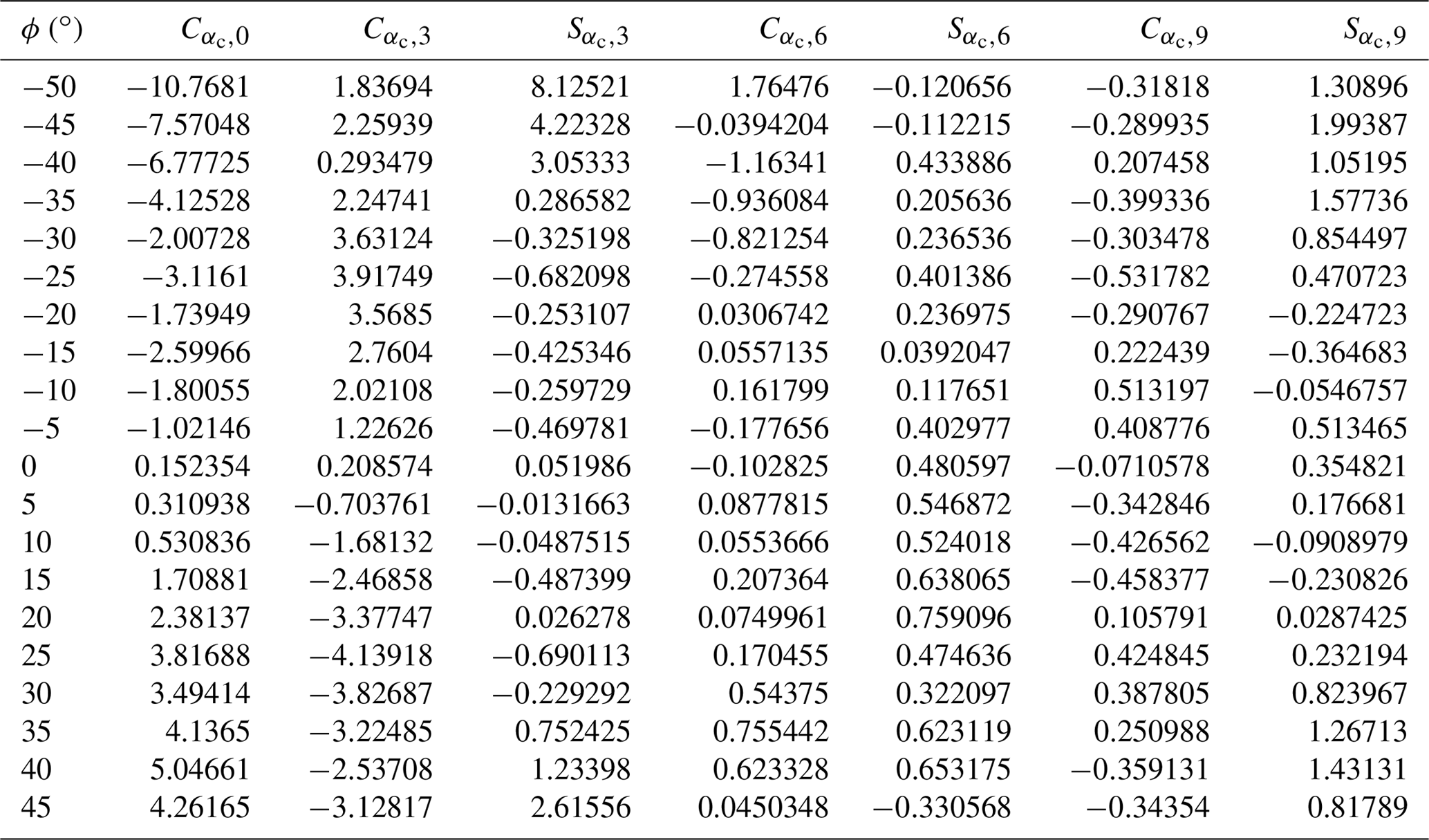
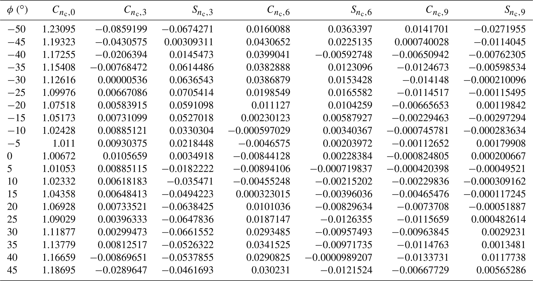
where n_c(α,ϕ), α_c(α,ϕ), and ϕ_c(α,ϕ) are α- and ϕ-dependent correction factors (note that there is a typo in V_3-D in M04), which are computed through Fourier series with coefficients C_f,i(ϕ) and S_f,i(ϕ) that are provided in the LUTs,

$$\begin{array}{}\text{(9)}& f_{\mathrm{c}}(\mathit{\alpha },\mathit{\varphi })=\sum _{i=\mathrm{0},\mathrm{3},\mathrm{6},\mathrm{9}}\left[C_{f_{\mathrm{c}},i}\left(\mathit{\varphi }\right)\cos \left(i\mathit{\alpha }\right)+S_{f_{\mathrm{c}},i}\left(\mathit{\varphi }\right)\sin \left(i\mathit{\alpha }\right)\right],\end{array}$$

where f_c(α,ϕ) is either n_c(α,ϕ), α_c(α,ϕ), or ϕ_c(α,ϕ). The LUTs are not given in M04 and so we provide them in Appendix A. The 3-D-corrected velocities are

$$\begin{array}{}\text{(10)}& {\displaystyle }{x}_{\mathrm{3}\text{-}\mathrm{D}}& {\displaystyle }=-V_{\mathrm{3}\text{-}\mathrm{D}}\cos {\mathit{\alpha }}_{\mathrm{3}\text{-}\mathrm{D}}\cos {\mathit{\varphi }}_{\mathrm{3}\text{-}\mathrm{D}},\text{(11)}& {\displaystyle }{y}_{\mathrm{3}\text{-}\mathrm{D}}& {\displaystyle }=-V_{\mathrm{3}\text{-}\mathrm{D}}\sin {\mathit{\alpha }}_{\mathrm{3}\text{-}\mathrm{D}}\cos {\mathit{\varphi }}_{\mathrm{3}\text{-}\mathrm{D}},\text{(12)}& {\displaystyle }{z}_{\mathrm{3}\text{-}\mathrm{D}}& {\displaystyle }=-V_{\mathrm{3}\text{-}\mathrm{D}}\sin {\mathit{\varphi }}_{\mathrm{3}\text{-}\mathrm{D}}.\end{array}$$

3 Sites and instrumentation

Measurements were collected from sonic anemometers mounted on three meteorological masts at two sites in Denmark: the Risø test site on the Zealand island and the Nørrekær Enge wind farm on northern Jutland (see Fig. 2). The Risø test site is over a slightly undulating terrain with a mix of cropland, grassland, artificial land, and coast (the Roskilde Fjord coastline is ≈250 m northwest of the turbine stands). The Nørrekær Enge wind farm is located ≈350 m southeast of the water body Limfjorden over flat terrain with a mix of croplands and grasslands.

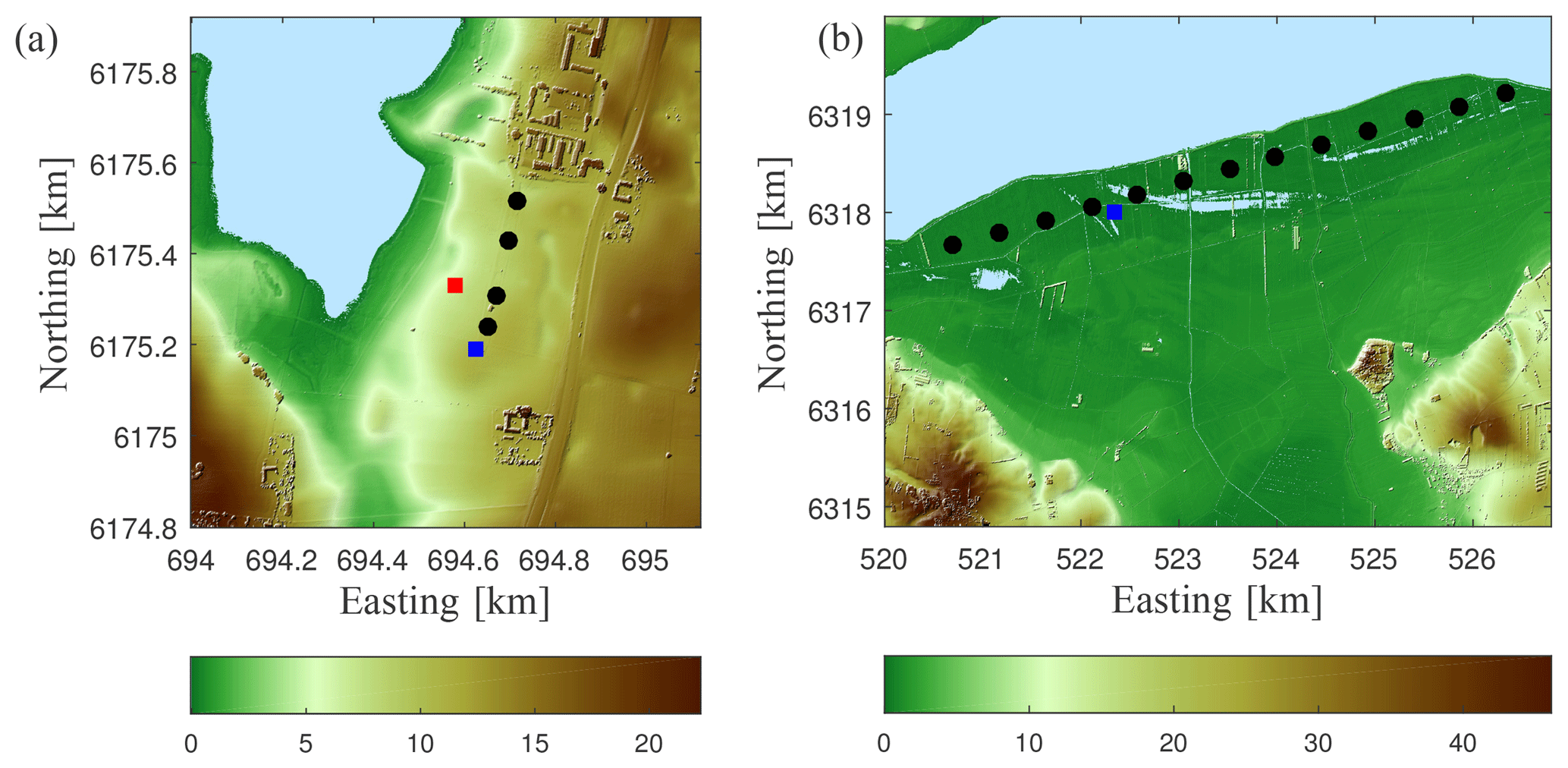
Figure 2 Locations of the sonic anemometer measurements. Wind turbines are indicated by black circles, masts with a CSAT3 by blue squares, and the mast with a USA-1 by a red square. Panel (a) shows the Risø test site and (b) the Nørrekær wind farm site. The color bar indicates the height above mean sea level in meters based on a digital surface elevation model (UTM32 WGS84).

At the Risø test site, a CSAT3 was mounted at 6.4 m above ground level (a.g.l.) on a 2.5 m boom on a 15 m tall tower. The boom was oriented 14^∘ from the north. The tower was a triangular lattice structure with a side length of 0.4 m at the measurement height. The data acquisition unit was placed on the western leg of the tower, just below the boom. From the point of view of the mast, turbines were located within the direction sector 16–29^∘.

Also at the Risø test site, but on a different mast, a USA-1 Basic was mounted at 16.5 m a.g.l. on a 2 m boom, which is oriented 10^∘ from the north, on a 54 m tall tower that is located west of the wind turbine stands. The tower is a square lattice structure 0.3 m wide from bottom to top. From the point of view of the mast, turbines are located within the direction sector 36–142^∘.

At the Nørrekær Enge wind farm, a CSAT3 was mounted at 76 m a.g.l. on a 3.1 m boom, which is oriented 192.5^∘ from the north, on a 80 m mast that is located southeast of the row of wind turbines between stands 4 and 5, numbered from left to right. From the point of view of the mast, these two turbines are located within the direction sector 281–40^∘. The closest turbine (4) is at 232 m and turbines are separated by 487 m. The mast is an equilateral triangular lattice structure with a width of 0.4 m at 80 m.

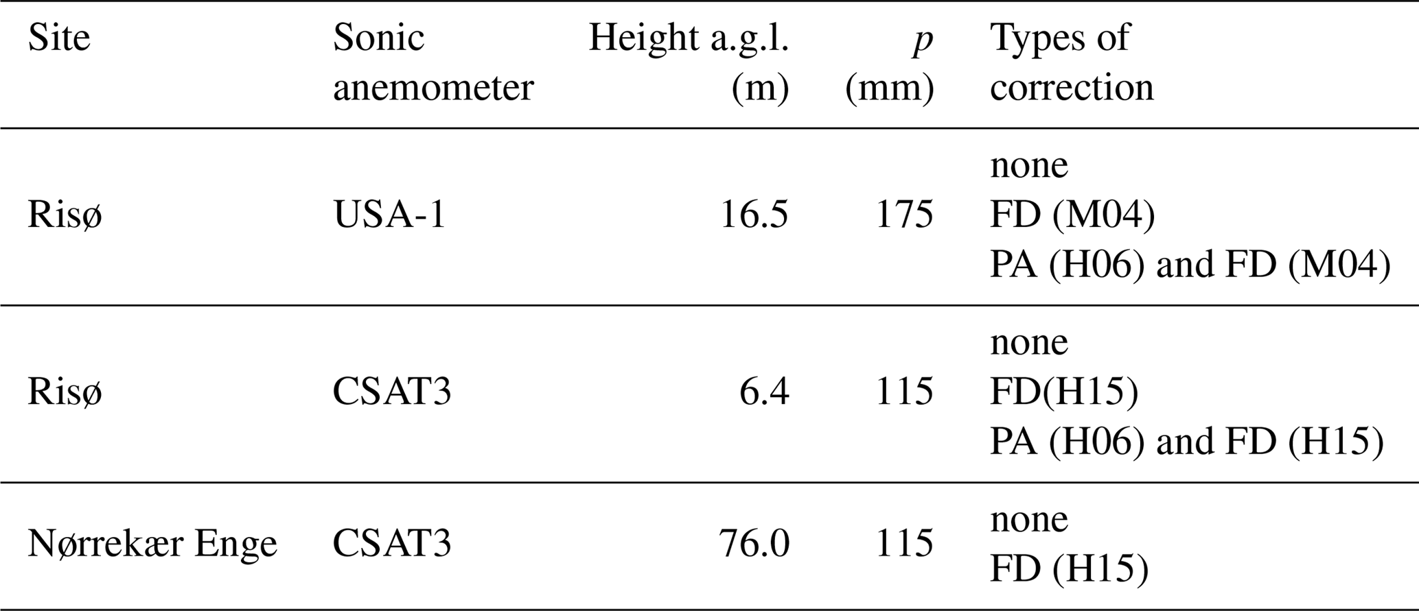
At all sites the sonic anemometers were mounted so that their north was aligned with the boom direction. Thus, wind directions are hereafter relative to the sonic anemometer orientation where 0^∘ is aligned with the boom. In Table 1, the specifications of the sonic anemometers at the two sites and the applied corrections are provided.

Table 1 Sonic anemometer specifications for each measurement site including the types of flow-distortion (FD) and/or path-averaging (PA) corrections applied. Due to the height of the instrument at Nørrekær Enge, we did not apply a PA correction as the error should be negligible.

4 Data treatments

For all sonic anemometers, we analyzed the time series of the three velocity components on a 10 min basis when U>3 m s⁻¹. We applied azimuth and tilt rotations to the time series so that u became aligned with the mean wind vector for each 10 min period. Finally, we computed all velocity spectra and co-spectra as well as the mean wind direction for each 10 min period. All mentions of direction hereafter refer to the 10 min mean relative to the boom orientation.

4.1 USA-1 at the Risø test site

The USA-1 measurements at Risø were sampled at 20 Hz. We used (a total of 25 401) 10 min time series of measurements conducted in 2014 in order to have sufficient data covering all directions. We did all spectra calculations on each the raw (non-corrected data), the 2-D-, and 3-D-corrected data. We also applied the path-length averaging correction by H06 to the 3-D-corrected data.

4.2 CSAT3 at the Risø test site

The CSAT3 measurements at Risø were taken between November 2013 and mid-January 2014, and sampled at 60 Hz. For the analysis, it was required that all recorded velocities had the manufacturer's quality signal equal to zero. Two velocity corrections were performed: the path-length averaging (H06) and the flow-distortion correction suggested by H15. After the quality signal filter, the amount of 10 min time series left were 2720.

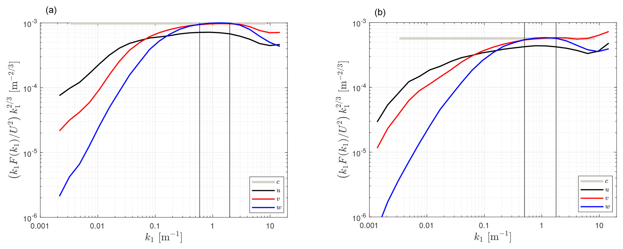
Figure 3 Ensemble-averaged, 3-D-corrected velocity spectra by the USA-1 at the Risø test site at 16.5 m for two directions intervals: one parallel 0±10^∘ (a) and another perpendicular 90±10^∘ (b) to the boom. A 0^∘ polynomial (c) was fit to the normalized w spectra within the wavenumber range indicated by black vertical lines.

4.3 CSAT3 at the Nørrekær Enge wind farm

The CSAT3 measurements at Nørrekær Enge were sampled at 10 Hz. We used (a total of 27 837) 10 min time series of measurements conducted in 2015, when the manufacturer's quality signal was equal to zero and no precipitation was recorded by a rain gauge on the mast. We also applied the flow-distortion correction suggested by H15.

5 Results

For the three sonic anemometers, we first show velocity spectra ensemble-averaged over two direction intervals: one parallel and another perpendicular to the boom direction. The wavenumber premultiplied spectra were normalized using the horizontal wind-speed magnitude, which, in our analysis, has been shown to reduce the scatter in the velocity spectra. To illustrate that within a wavenumber range, the velocity spectra ratios approach the theoretical spectral slopes of the inertial subrange closely, the wavenumber premultiplied spectra were multiplied by $k_{\mathrm{1}}^{\mathrm{2}/\mathrm{3}}$ (in contrast to the idealized wavenumber premultiplied spectra in Fig. 1) so that the inertial subrange can be distinguished as a flat region.

Second, for the selected wavenumber range, the velocity spectra ratios were computed for each 10 min sample and the statistics of these ratios were calculated for a wind direction range where the influence of the mast should be the lowest and incorporated in Table 2. We also show all 10 min velocity spectra ratios as a function of direction (with and without flow corrections). For the specific case of the USA-1, we show the ratios of the velocity variances as function of direction as well.

Further, to assess whether or not within the selected wavenumber range the velocity spectra conformed to the expected behavior within the inertial subrange, we also filtered out “poorly” behaved spectra (e.g., from those winds affected by wind turbine wakes) by assuring that within the selected wavenumber range, both the slope of the w velocity spectrum was $-\mathrm{5}/\mathrm{3}\pm \mathrm{0.003}$ and $|F_{uw}/\sqrt{F_u{F}_w}|<\mathrm{0.02}$ (i.e., a uw co-covariance test narrowing for isotropy, see Sect. 2.1) for each 10 min sample. The slope was computed by fitting a 0^∘ polynomial to the normalized w spectra within the selected wavenumber range. We call these two latter tests “sharpened” criteria in Table 2.

5.1 USA-1 at the Risø test site

Figure 3 shows two examples of 3-D-corrected velocity spectra, ensemble-averaged over two direction intervals for measurements of the USA-1 at the Risø test site. It is seen that for both direction intervals, the region in which the w velocity spectrum becomes flat is within the same wavenumber range ($\mathrm{0.5}{\mathrm{m}}^{-\mathrm{1}}\le k_{\mathrm{1}}\le \mathrm{1.8}$ m⁻¹). It is also observed that the spectra of the directions parallel to the sonic orientation have higher power spectral density than those of the directions perpendicular because for the latter, the spectra are influenced by the fjord. Thus, we assumed at first that each 10 min spectrum can be analyzed within the same range, irrespective of the wind conditions; this assumption is later tested using the sharpened criteria.

Figure 4a shows the w to u spectra ratio for each non-corrected and 3-D-corrected 10 min. It is clearly seen that the non-corrected data approach a ratio close to 1, whereas the 3-D-corrected data approach 4∕3. Figure 4b shows the v to u spectra ratio for each non-corrected and 3-D-corrected 10 min. It is shown that both sets of data approach a ratio close to 4∕3, although the 3-D correction seems to generally increase the ratio. The u and v spectra did not change much after the 3-D correction (not shown). Table 2 provides the computed velocity spectra ratios within the inertial subrange for the direction interval where there was no direct influence by the mast or winds were not affected by turbine wakes and for each the non-corrected measurements, the 3-D corrected, and the path-length averaging- and 3-D-corrected measurements. It is important to note that for all correction types, the v to u spectra ratio is close to 4∕3 and that by applying the sharpened criteria, the statistics on both spectra ratios did not change significantly. The effect of path-length averaging (H06) on the spectra ratios was opposite to that of the 3-D correction but rather small.

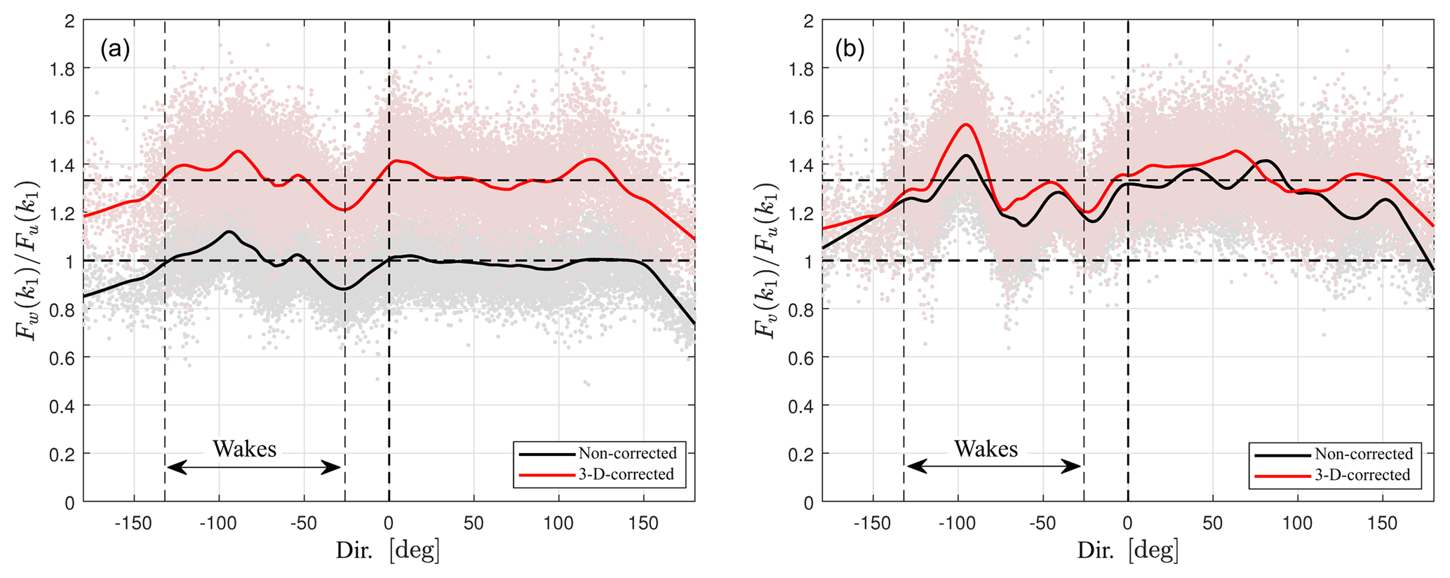
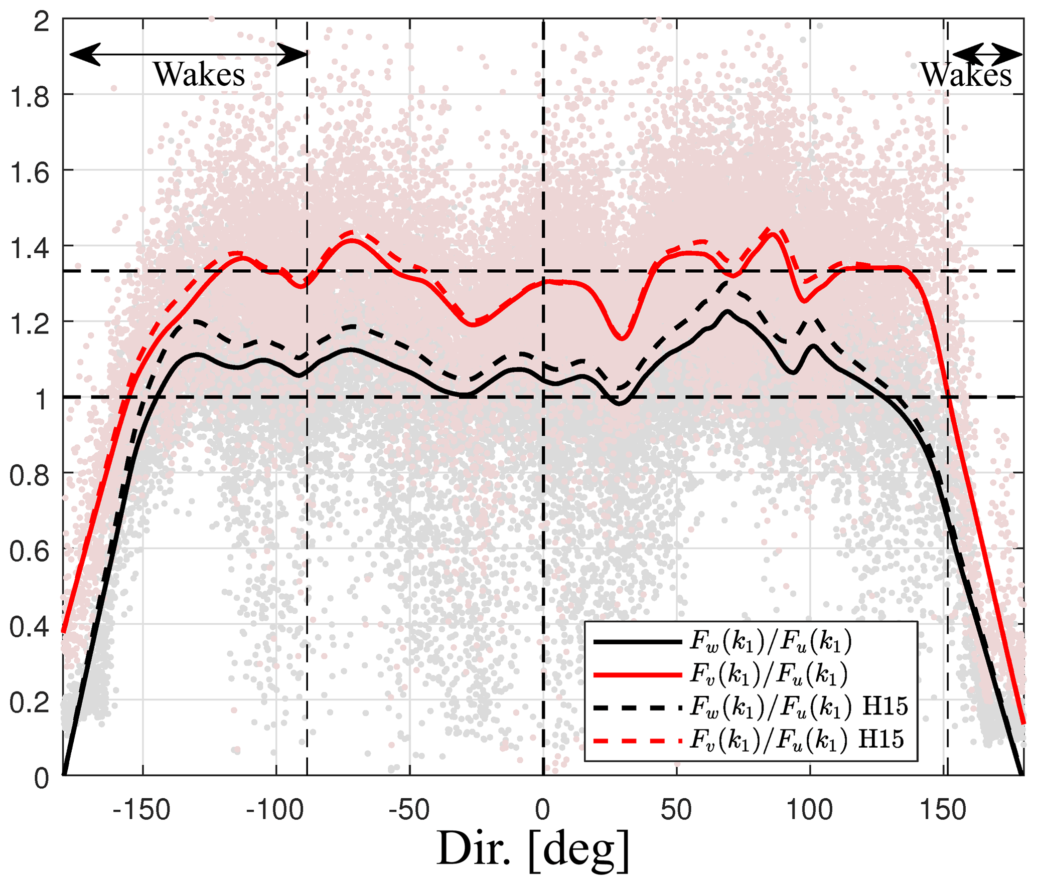
Figure 4 Velocity spectra ratios by the USA-1 at the Risø test site as function of wind direction. (a) w to u velocity and (b) v to u velocity spectra ratios for the non- and 3-D-corrected data. Each 10 min ratio is shown in markers and the solid lines show a loess fit of the scatter. The thick dashed vertical line indicates the 0^∘ direction, the thin dashed vertical lines indicate the sector with possible turbine wakes, and two dashed horizontal lines the values 1 and 4∕3. The standard error of the fit to the 3-D-corrected w to u velocity spectra ratios is within 0.0020–0.0031.

Table 2 Computed velocity spectra ratios within the inertial subrange for the direction range within ±120^∘ and excluding directions possibly affected by turbine wakes. The mean value is given ± 1 standard deviation.

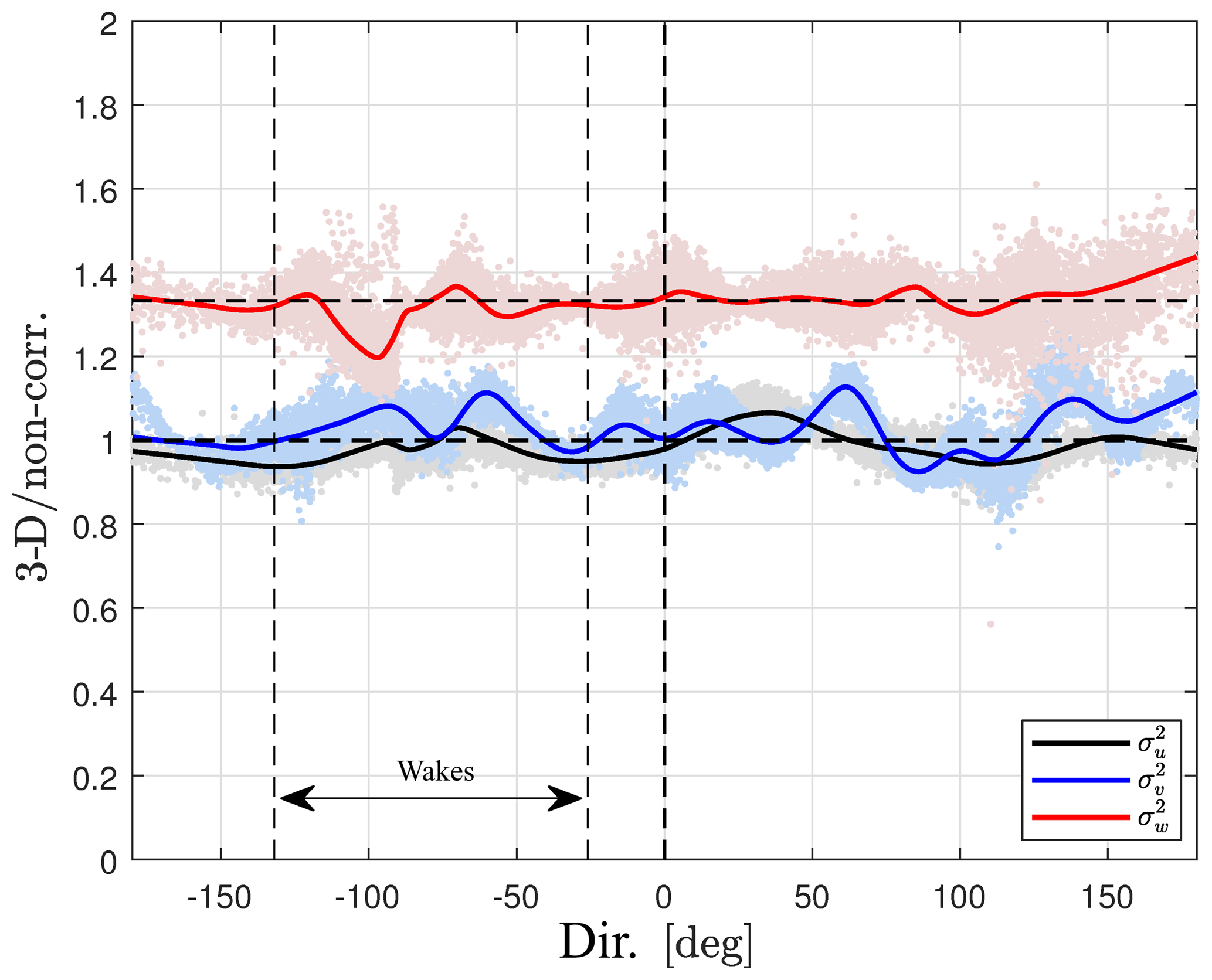
Figure 5 shows the ratio of the 3-D-corrected to the non-corrected velocity variances as function of wind direction. It is clearly seen that the 3-D correction did not only change the spectral density of w within the inertial subrange but that it increased the spectral density at all wavenumbers, and so the 3-D-corrected variance is 33.33 % higher than the non-corrected one. As expected, the 3-D correction did not change the u and v variances much.

Figure 5 Ratios of the 3-D-corrected to the non-corrected velocity variances by the USA-1 at the Risø test site as function of the wind direction. Each 10 min ratio is shown in markers and the lines show a moving average of the scatter. Horizontal and vertical dashed lines as in Fig. 4.

5.2 CSAT3 at the Risø test site

From the investigated sonic anemometers, the CSAT3 at Risø had the lowest measurement height. Since the velocity spectra scale with height, the inertial subrange was expected to be within a range of higher wavenumbers compared to those from the other two sonic anemometers. The wavenumber range at which the premultiplied velocity spectra from this sonic anemometer showed an approximately flat range is $k_{\mathrm{1}}=[\mathrm{2},\mathrm{5}]$ m⁻¹ (see Fig. 6). Such high wave numbers might be affected by white noise from the data acquisition itself. The upper limit of the k₁ interval chosen for analysis was therefore limited, particularly for the u and v components (refer to Appendix B for an explanation of why each velocity component is affected differently by noise), which caused the spectral slope to be greater than $-\mathrm{5}/\mathrm{3}$.

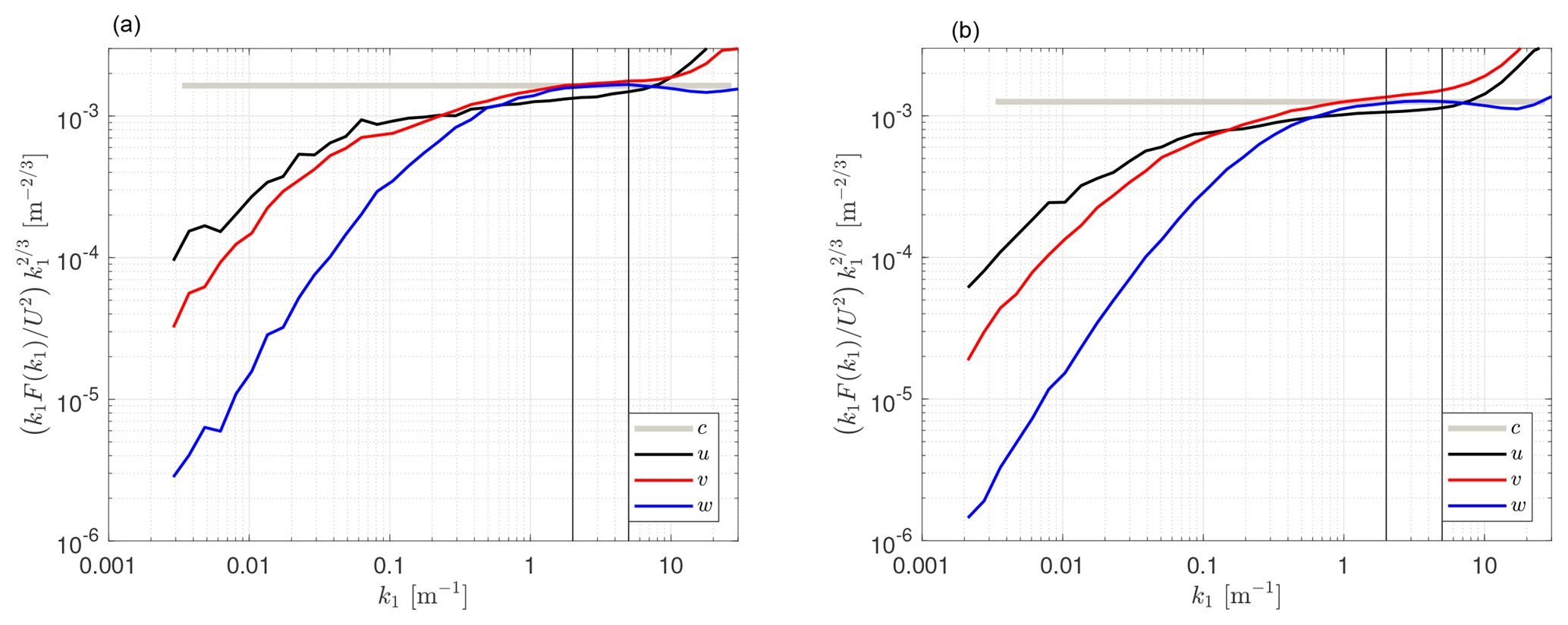
Figure 6 Similar to Fig. 3, but for the CSAT3 at the Risø test site. For the direction parallel to the boom (a), the average spectra were computed over 72 different 10 min samples, whereas for the directions perpendicular to the boom (b), the average was based on 453 different 10 min samples.

Figure 7 illustrates the computed velocity-component spectra ratios. Both F_w(k₁)∕F_u(k₁) and F_v(k₁)∕F_u(k₁) showed very low values for absolute directions greater than ≈150^∘. For directions more aligned to the boom, the ratios varied between 1.0 and 1.6 (Fig. 7a). For most of the directional intervals, the ratio F_v(k₁)∕F_u(k₁) was clearly higher than the F_w(k₁)∕F_u(k₁) ratio. Due to the large difference in heights between this sonic anemometer and the hub height of the turbines in the site and because the closest turbine to the mast was not in operation during the acquisition of the sonic anemometer measurements, we judged that the wake effects are negligible for the computed ratios in Table 2. As shown in the table, the results for the mean velocity ratios were insensitive to the poor spectra filter. As for the USA-1 at Risø, for all correction types and criteria used, the v to u spectra ratio was close to 4∕3.

In Fig. 7b, we show the loess fit for the cases: no correction, H15 correction, and the combination of the H06 and H15 corrections. Whereas the H15 correction increased the ratios, by adding the H06 correction, the ratio was reduced. It can be observed that the effect of path-length averaging (H06) was opposite to that of transducer shadowing (H15). As discussed before, F_u is attenuated more than F_v and F_w by path-length averaging in the inertial subrange. Therefore, when path-length averaging was accounted for, the ratios reduced.

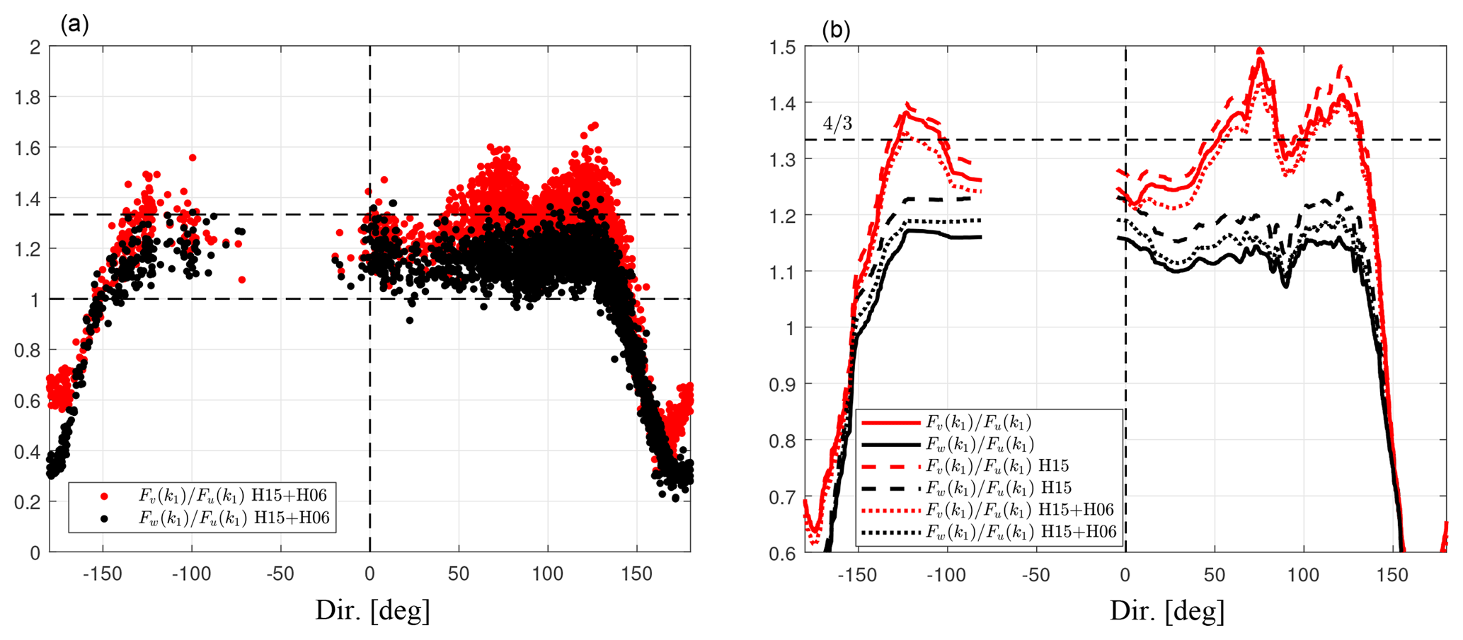
Figure 7 Velocity spectra ratios by the CSAT3 at the Risø test site as a function of wind direction for each 10 min period after applying the corrections in H15 and H06 (a) and loess fits of the scatter (b). Horizontal and vertical dashed lines as in Fig. 4. The standard error of the fit to the w to u velocity spectra ratios is within 0.0024–0.0072.

5.3 CSAT3 at the Nørrekær Enge wind farm

Figure 8 shows two examples of normalized velocity spectra, ensemble-averaged over two direction intervals for measurements of the CSAT3 at Nørrekær Enge as well as the polynomial fit within a chosen wavenumber range. The wavenumber range was limited to exclude noise apparent at higher wavenumbers (k₁>1 m⁻¹). Similar to the velocity spectra measured by the CSAT3 at the Risø test site, the w spectrum closely followed the u spectrum and the v spectrum showed the highest spectral density within the inertial subrange ($\mathrm{0.38}{\mathrm{m}}^{-\mathrm{1}}\le k_{\mathrm{1}}\le \mathrm{0.88}$ m⁻¹).

Figure 8 Similar to Fig. 3 but for the CSAT3 at the Nørrekær Enge wind farm.

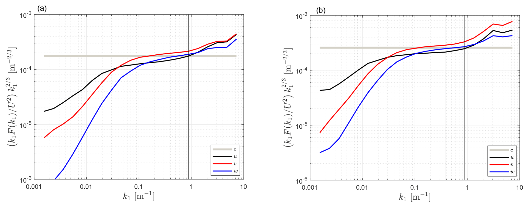
Figure 9 shows the w and v to u spectra ratios for each 10 min. The result is very similar to that for the CSAT3 at the Risø test site where within a range of directions of $\pm \mathrm{150}{}^{\circ }$, the w to u spectra ratios were close to 1, whereas the v to u spectra ratios were close to 4∕3. The boom and mast structure had a greater effect on the CSAT3 at the Nørrekær Enge wind farm than at the Risø site as expected due to the setup. For both sites, the effect of the boom and mast at directions close to $\pm \mathrm{180}{}^{\circ }$ was very similar. In agreement with the findings using the CSAT3 at Risø (Sect. 5.2), the H15 correction increased both the F_w(k₁)∕F_u(k₁) and F_v(k₁)∕F_u(k₁) spectra ratios (particularly for the former) but not enough to reach the 4∕3 value for F_w(k₁)∕F_u(k₁) (see Table 2). As for the previous two cases, for all correction types and criteria, the v to u spectra ratio was close to 4∕3.

Figure 9 CSAT3 velocity spectra ratios with wind direction at the Nørrekær Enge wind farm. Horizontal and vertical dashed lines as in Fig. 4. The standard error of the fit to the w to u velocity spectra ratios is within 0.0038–0.0086 for the H15 correction.

6 Discussion

6.1 Uncertainties

The aim of the spectral analysis displayed in Figs. 3, 6, and 8 was to find the optimal inertial subrange for each site and setup. A high-end limitation to this interval can be the presence of white noise in the spectra, which would tend to reduce the examined spectral ratios. For the velocity spectra at all three locations, we observe that the high-frequency w noise is the lowest of the three velocity components and is proportionally lower for the CSAT3 than for the USA-1, which is consistent with its larger path elevation angle as explained theoretically in Appendix B. According to the theory, the noise in the v and u spectra should be identical irrespective of the wind direction relative to the boom. The data showed deviations from this prediction. In addition, for the Risø CSAT3 setup, numerous tests with regard to both wavenumber and frequency ranges were performed, resulting in only very slight changes to the results in Fig. 7 (not shown). Another test for the robustness of the results was performed by selecting only those spectra that showed close to perfect inertial subrange behavior within the selected wavenumber range (a close to $-\mathrm{5}/\mathrm{3}$ slope for F_w(k₁) and a low uw co-covariance, see “Sharpened criteria” in Table 2), which increased the CSAT3 ratios at Risø by 0.6 %–1.6 % only.

The choice of thresholds for the sharpened criteria compromised the amount of data left for the analysis; about 4 %, 25 %, and 1 % of the original amount of 10 min periods for the USA-1 at Risø, CSAT3 at Risø, and the CSAT3 at Nørrekær Enge, respectively. The choice, however, did not change the velocity spectra ratios significantly. The softening of the values to, e.g., 0.03 and 0.2 for the w spectral slope and the uw co-covariance, respectively, resulted in a change of the w to u velocity spectra ratio of ≈0.6 % for the USA-1, ≈1.5 % for the CSAT3 at Risø, and ≈0.8 % for the CSAT3 at Nørrekær Enge, only.

Another potential source of error comes from the choice of coordinate system in which the spectra were calculated. Here, we used two rotations for each 10 min block of data, whereas Horst et al. (2015) used the planar-fit coordinate system by Wilczak et al. (2001). We tested whether an error in rotation angle would change the results. This was done by rotating the sonic anemometer measurements of the velocity components and applying an isotropic inertial subrange 3-D spectral velocity tensor, as in H06, to calculate the nominal component spectra for this configuration. A change of up to $\pm \mathrm{5}{}^{\circ }$ in the rotation angles of the sonic anemometer about vertical and transverse axes resulted in a less than 0.7 % reduction in the spectral ratio; therefore, we consider rotation-related errors to be of no importance.

6.2 Implications

We base our analysis on theoretical arguments about the w and v to u velocity spectral ratios, which should be equal to 4∕3 within the inertial subrange. We find such ratios by applying the 3-D wind-tunnel-derived flow-distortion corrections to atmospheric velocity measurements performed with a USA-1 (Table 2), whereas applying a flow-distortion correction to the CSAT3 results in ratios within the range 1.12–1.19. If we assume that the discrepancy to 4∕3 is due to remaining uncorrected flow distortion and further, that flow distortion affects the observed frequencies equally, which is an assumption supported by the results presented in Huq et al. (2017), the imperfect ratios correspond directly to an underestimation in the velocity variances. Since our results do not indicate how each velocity component is affected, it is still difficult to directly use the results presented here to correct the variances. However, some qualitative comparisons can be made. If, for example, the u and v velocity components are measured with no error, the observed ratios of 1.12–1.19 can only turn into 4∕3 if the w variance is increased by 18 %–26 %, which means that the w component itself should increase by 8 %–12 %. This error range is in agreement with the results by Frank et al. (2016), but higher than the error suggested by Huq et al. (2017). If we, on the other hand, assume equal errors on all velocity components (positive for u and v, and negative for w) the ideal ratio of 4∕3 can be reached with a 4 %–6 % correction on the velocity components. These examples illustrate that our method can be a useful tool for judging whether flow-distortion corrections of a particular sonic anemometer are adequate or not but that it cannot be used directly to quantify the error.

Another clear result from the presented analyses concerns the difference between observed mast, boom, and instrument shadowing for the USA-1 and CSAT3; even from narrow masts and relatively long supporting booms, the mast influence is more marked for the CSAT3 than for the USA-1. Whereas Foken (2008) recommended the use of sonic anemometers without a pole directly under the sonic measurement volume for atmospheric turbulence research, we stress here that this statement can at best be valid only for a limited wind direction interval. For anemometers mounted on bulky walk-up towers, the direction interval where data will be biased from the tower will likely be much larger. We further stress that a sonic anemometer that cannot reproduce a 4∕3 ratio in the inertial subrange cannot be trusted to give accurate observations of all velocity components, provided that an inertial subrange is clearly apparent. Despite a higher ratio of transducer diameter to path length, which is sometimes used as a sonic anemometer quality marker, the USA-1, including the wind-tunnel-derived flow-distortion correction, therefore comes out better from our analysis.

6.3 Sonic anemometry quality assessments

We suggest that the spectral ratios of velocity components within the inertial subrange are a valuable addition to field tests and wind-tunnel calibrations. The advantage of the presented method is that any sonic anemometer can be tested provided that inertial subrange characteristics are expected from the particular measurements. Unlike sonic anemometer intercomparisons, where ideal flat and uniform sites are preferred (Mauder et al., 2007), the spectral ratio method did not seem to be sensitive to the spatial and flow heterogeneity at the sites used here.

As mentioned above, a limitation to our method is that the accuracy of individual velocity components cannot be assessed; the 3-D-corrected observations from the USA-1, although almost perfect in terms of the 4∕3 ratio, might still be inaccurate if all three velocity components are biased. Looking ahead, a reference for sonic anemometer measurements could be found in small-volume lidar anemometry (Abari et al., 2015), which is free of flow distortion.

6.4 Can wind-tunnel-based calibrations be trusted in atmospheric turbulence?

Starting with Högström and Smedman (2004), the validity of wind-tunnel calibrations for sonic anemometer has been questioned for applications in the turbulent atmosphere. Using large-eddy simulation results, Huq et al. (2017) argued that the magnitude of the flow-distortion error caused by the sonic anemometer is smaller under turbulent conditions than under quasi-laminar flow while also showing that the flow-distortion error does not depend on the frequency of the fluctuations. Taken the latter result to the extreme low-frequency limit, these two results appear inconsistent. In this study, the application of a flow-distortion correction for the USA-1, derived from wind-tunnel observations, led to near-perfect spectral ratios in the inertial subrange, whereas that by H15, based on both field tests and wind-tunnel observations, did not. Provided that the wind-tunnel reference instrument is accurate and the blockage ratio in the tunnel is small, we argue that flow distortion can be correctly quantified also in quasi-laminar flow because the turbulence eddy sizes are significantly larger than the transducer size. In this way, the atmospheric turbulent flow appears laminar as seen from the transducer. An explanation for the deviation of the results between sonic anemometer observations in wind tunnel and field tests in Högström and Smedman (2004) could also be that the velocities recorded by the early Gill sonic anemometers showed a marked temperature dependence (Mortensen and Højstrup, 1995).

7 Conclusions

The accuracy of atmospheric turbulence measurements performed by sonic anemometers was investigated using two instruments, a CSAT3 and a USA-1, at two locations in Denmark. This was achieved by computing velocity spectra ratios within the inertial subrange. It was found that 3-D flow corrections applied to measurements from the USA-1 helped in recovering the 4∕3 ratio of the w to the u velocity spectra that is expected within the inertial subrange. The 3-D corrections also have a strong influence on the estimated w variances, which are systematically found to be ≈33.33 % higher than those of the uncorrected measurements. For the CSAT3, which is commonly categorized as the sonic anemometer closest to being a distortion-free instrument, the ratio of the w to the u velocity spectra is ≈1.1 without applying a flow-distortion correction. Using a previously proposed flow-distortion correction, the ratios changed to ≈1.15 on average, indicating that more work is needed to correctly quantify the flow distortion of this instrument. We propose to perform this type of analysis, in addition to field site intercomparisons and wind-tunnel calibrations, to assess the accuracy of sonic anemometer measurements. We also found that the influence of the mast, boom, and the instrument itself was higher on the CSAT3 compared to the USA-1 measurements.

Appendix A: Metek USA-1 3-D flow-distortion corrections

Table A1 LUT for α_c(α,ϕ).

Table A2 LUT for ϕ_c(α,ϕ).

Table A3 LUT for n_c(α,ϕ).

Appendix B: Sonic anemometer noise

The transformation matrix to convert the three sonic path velocities $\mathbf{s}=(s_{\mathrm{1}},s_{\mathrm{2}},s_{\mathrm{3}})$, which are assumed positive from the lower to the upper acoustical transducer, to right-handed orthogonal velocity components $\mathit{u}=(u_{\mathrm{1}},u_{\mathrm{2}},u_{\mathrm{3}})=(u,v,w)$, with u in the direction of the horizontal boom, v horizontal and transverse to u, and w in the vertical direction and positive upwards, is

$$\begin{array}{}\text{(B1)}& T=\left(\begin{array}{ccc}-{\displaystyle \frac{\mathrm{2}\sec {\mathit{\varphi }}_{\mathrm{p}}}{\mathrm{3}}}& {\displaystyle \frac{\sec {\mathit{\varphi }}_{\mathrm{p}}}{\mathrm{3}}}& {\displaystyle \frac{\sec {\mathit{\varphi }}_{\mathrm{p}}}{\mathrm{3}}}\\ \mathrm{0}& {\displaystyle \frac{\sec {\mathit{\varphi }}_{\mathrm{p}}}{\sqrt{\mathrm{3}}}}& -{\displaystyle \frac{\sec {\mathit{\varphi }}_{\mathrm{p}}}{\sqrt{\mathrm{3}}}}\\ {\displaystyle \frac{\csc {\mathit{\varphi }}_{\mathrm{p}}}{\mathrm{3}}}& {\displaystyle \frac{\csc {\mathit{\varphi }}_{\mathrm{p}}}{\mathrm{3}}}& {\displaystyle \frac{\csc {\mathit{\varphi }}_{\mathrm{p}}}{\mathrm{3}}}.\end{array}\right),\end{array}$$

where ϕ_p is the path elevation angle, so

$$\begin{array}{}\text{(B2)}& u_i=T_{ij}{s}_j,\end{array}$$

and we also assume the sonic anemometer paths to be oriented in the azimuthal direction like the CSAT3 or the USA-1.

Suppose now that the sonic anemometer signals are composed of uncorrelated, white noise $\langle s_i{s}_j\rangle ={\mathit{\sigma }}_s^{\mathrm{2}}{\mathit{\delta }}_{ij}$, where δ is the Kronecker delta symbol and ${\mathit{\sigma }}_s^{\mathrm{2}}$ is the noise variance. The resulting noise on the orthogonal velocity components then becomes

$$\begin{array}{ll}{\displaystyle }\langle u_i{u}_j\rangle & {\displaystyle }=\langle T_{ik}{s}_k{T}_{jl}{s}_l\rangle ={\mathit{\sigma }}_s^{\mathrm{2}}{T}_{ik}{\mathit{\delta }}_{kl}{T}_{jl}={\mathit{\sigma }}_s^{\mathrm{2}}{T}_{ik}{T}_{jk}\\ \text{(B3)}& {\displaystyle }& {\displaystyle }={\mathit{\sigma }}_s^{\mathrm{2}}\left(\begin{array}{ccc}{\displaystyle \frac{\mathrm{2}{\sec }^{\mathrm{2}}{\mathit{\varphi }}_{\mathrm{p}}}{\mathrm{3}}}& \mathrm{0}& \mathrm{0}\\ \mathrm{0}& {\displaystyle \frac{\mathrm{2}{\sec }^{\mathrm{2}}{\mathit{\varphi }}_{\mathrm{p}}}{\mathrm{3}}}& \mathrm{0}\\ \mathrm{0}& \mathrm{0}& {\displaystyle \frac{{\csc }^{\mathrm{2}}{\mathit{\varphi }}_{\mathrm{p}}}{\mathrm{3}}}\end{array}\right).\end{array}$$

Since the u and v components behave identically in terms of noise, the error is also given by Eq. (B3) if the components are rotated into the mean wind direction coordinate system and as long as the wind vector is horizontal. Also, since the noise is assumed white, the relative strengths of noise-dominated spectra will also follow Eq. (B3). The ratio between the horizontal and vertical spectra will therefore increase rapidly with path elevation angle as shown in Fig. B1. The unit ratio occurs for ${\mathit{\varphi }}_{\mathrm{p}}={\tan }^{-\mathrm{1}}\left({\mathrm{2}}^{-\mathrm{1}/\mathrm{2}}\right)\approx \mathrm{35}{}^{\circ }$ or at a path zenith angle of $\mathrm{90}{}^{\circ }-{\mathit{\varphi }}_{\mathrm{p}}\approx \mathrm{55}{}^{\circ }$. This is also the path elevation angle where the sum of the three component variances obtains a minimum of exactly 3 times ${\mathit{\sigma }}_s^{\mathrm{2}}$. Because of flow distortion, sonic anemometers do not have such a low path elevation angle.

Figure B1 The ratio of the noise level in the horizontal velocity components to the vertical one as a function of path elevation angle.