the Creative Commons Attribution 4.0 License.
the Creative Commons Attribution 4.0 License.
 | 23 Apr 2019
FRESCO-B: a fast cloud retrieval algorithm using oxygen B-band measurements from GOME-2
Marine Desmons
Ping Wang
Piet Stammes
L. Gijsbert Tilstra
The FRESCO (Fast Retrieval Scheme for Clouds from the Oxygen A band) algorithm is a simple, fast and robust algorithm used to retrieve cloud information in operational satellite data processing. It has been applied to GOME-1 (Global Ozone Monitoring Experiment), SCIAMACHY (Scanning Imaging Absorption Spectrometer for Atmospheric Chartography), GOME-2 and more recently to TROPOMI (Tropospheric Monitoring Instrument). FRESCO retrieves effective cloud fraction and cloud pressure from measurements in the oxygen A band around 761 nm. In this paper, we propose a new version of the algorithm, called FRESCO-B, which is based on measurements in the oxygen B band around 687 nm. Such a method is interesting for vegetated surfaces where the surface albedo is much lower in the B band than in the A band, which limits the ground contribution to the top-of-atmosphere reflectances. In this study we first perform retrieval simulations. These show that the retrieved cloud pressures from FRESCO-B and FRESCO differ only between −10 and +10 hPa, except for high, thin clouds over vegetation where the difference is larger (about +15 to +30 hPa), with FRESCO-B yielding higher pressure. Next, inter-comparison between FRESCO-B and FRESCO retrievals over 1 month of GOME-2B data reveals that the effective cloud fractions retrieved in the O2 A and B bands are very similar (mean difference of 0.003), while the cloud pressures show a mean difference of 11.5 hPa, with FRESCO-B retrieving higher pressures than FRESCO. This agrees with the simulations and is partly due to deeper photon penetrations of the O2 B band in clouds compared to the O2 A-band photons and partly due to the surface albedo bias in FRESCO. Finally, validation with ground-based measurements shows that the FRESCO-B cloud pressure represents an altitude within the cloud boundaries for clouds that are not too far from the Lambertian reflector model, which occurs in about 50 % of the cases.
- Article
(2142 KB) - Full-text XML
- BibTeX
- EndNote


The Global Ozone Monitoring Experiment-2 (GOME-2) is a spectrometer flying on the MetOp series of satellites: on MetOp-A since 2006, on MetOp-B since 2012 and on MetOp-C, which was launched in November 2018. The GOME-2 instruments sense the backscattered Earth radiance and solar irradiance in the ultraviolet and visible part of the spectrum (240–790 nm) with a spectral resolution between 0.26 and 0.51 nm. The primary goal of GOME-2 measurements is the study of ozone as well as atmospheric trace gases and pollutants (e.g. nitrogen dioxide, sulfur dioxide, water vapour, bromine oxide). The trace-gas retrieval algorithms rely on information on cloud properties for each ground pixel. Indeed, clouds strongly affect trace-gas retrievals from satellite measurements because of their shielding effect, albedo effect and in-cloud absorption effect (Stammes et al., 2008). Therefore, in order to ensure good-quality trace-gas retrievals, it is very important to retrieve various cloud properties; specifically, the cloud top height, cloud geometrical thickness, cloud fraction, cloud optical thickness and the number of cloud layers (Boersma et al., 2004).
From a larger perspective, clouds are a key component of the Earth's climate system through their role in the Earth's hydrological cycle and radiation balance. Global observation and description of clouds is necessary to understand and properly depict their multiple overall effects. This is particularly true in the context of the climate change we are experiencing. In particular, the question of whether the coverage of different cloud types will change or if the partition of low-level versus high-level clouds – which have different and sometimes opposite radiative effects – will change is a crucial one. This is recognised as one of the major challenges in climate change predictions (Bony and Dufresne, 2005; Andrews et al., 2012; Vial et al., 2013).
The usage of the oxygen absorption for the retrieval of cloud pressure has already been studied for several decades. Indeed, O2 is well mixed in the atmosphere and the degree of O2 absorption can be related to a certain atmospheric path length. Above a bright surface, as a cloud acts in first approximation, O2 absorption that affects solar radiation backscattered towards a space-borne sensor is mainly related to the scene height (the cloud height in our case). Such methods using reflected sunlight in oxygen absorption bands depend very weakly on the pressure and temperature vertical profiles. They do not suffer from a lack of sensitivity in the case of low clouds and are not sensitive to temperature inversions like retrievals with infrared measurements. The use of the oxygen A band for remote sensing of cloud properties has been extensively studied (Wu, 1985; Fischer and Grassl, 1991; Kuze and Chance, 1994) and used in airborne campaigns (Fischer et al., 1991) and satellite missions (Vanbauce et al., 1998; Koelemeijer et al., 2001; Fournier et al., 2006; Lindstrot et al., 2006; Preusker et al., 2007; Lelli et al., 2012), demonstrating its capability of retrieving an apparent cloud pressure using different sensors with narrow spectral bands centred on the oxygen A-band region. However, the use of the oxygen B band for such retrievals remains quite limited, usually in association with measurements in the A band (Kuze and Chance, 1994; Yang et al., 2013) or applied to the retrieval of aerosols or vegetation properties (Marshak and Knyazikhin, 2017; Xu et al., 2017). In this paper, we propose a new version of the Fast Retrieval Scheme for Clouds from the Oxygen A band (FRESCO) algorithm, called FRESCO-B, which is based on measurements in the B band. Such a method is interesting for vegetated surfaces. Indeed for this type of surface, the surface reflectance is much lower in the B band than in the A band (Tilstra et al., 2017), limiting the ground contribution to the top-of-atmosphere (TOA) measured reflectances.
This paper is organised as follows. In Sect. 2, we present the FRESCO algorithm and our motivations to apply it in the oxygen B band. In Sect. 3, we describe the oxygen A and B bands, as well as the FRESCO-B retrieval method. In Sect. 4, we perform simulations of cloud retrievals in the oxygen A and B bands. In Sect. 5, we apply FRESCO-B to GOME-2 data and validate the results by performing comparisons with FRESCO and with ground-based measurements. We conclude this study in Sect. 6.
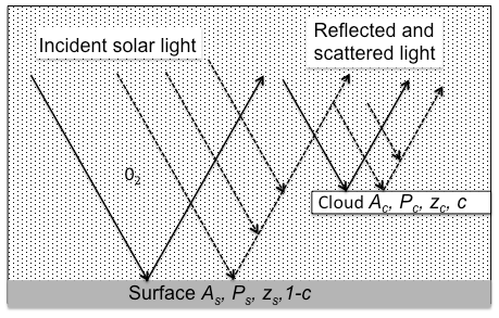
Figure 1The atmospheric radiation model used in the FRESCO retrieval algorithm. Three light paths are considered: (1) from sun to surface to satellite, (2) from sun to cloud to satellite (1–2: solid lines) and (3) from sun to atmosphere to satellite according to single Rayleigh scattering (dashed lines). The pixel is partly cloudy, with c the effective cloud fraction, and partly clear. As, Ps and zs stand, respectively, for the surface albedo, pressure and altitude, while Ac, Pc and zc indicate, respectively, the cloud albedo, pressure and altitude.
In the FRESCO algorithm (Koelemeijer et al., 2001; Wang et al., 2008), information on cloud pressure and the effective cloud fraction is derived from the reflectances in three 1 nm wide windows situated in and around the O2 A band. The algorithm fits a simulated reflectance spectrum to the measured reflectance spectrum in the three windows: namely 758–759, 760–761 and 765–766 nm. The atmospheric model used, shown in Fig. 1, is based on the independent pixel approximation: the top-of-atmosphere simulated reflectances (Rsim) are computed as the weighted sum of the reflectances of the cloud-free and cloudy parts of the pixel, using the cloud fraction for the weight. The atmosphere above the ground surface or cloud is treated as an absorbing (due to oxygen) and purely Rayleigh-scattering medium. The simulated reflectances can be written as follows (Wang et al., 2008):
where c is the effective cloud fraction while Ac and As stand for the cloud and surface albedo. Rc, Tc and Rs, Ts are the single Rayleigh-scattering reflectances and transmittances of the cloudy and cloud-free part of the pixel, respectively. The transmission and Rayleigh-scattering reflectances are precalculated as a function of the solar zenith angle (SZA), viewing zenith angle (VZA), azimuth difference, wavelength and pressure level (Pc, Ps). The transmission and reflectance spectra are calculated using a line-by-line method using the line parameters from HITRAN2016 (Gordon et al., 2017) and then convolved using the instrument spectral response function at the measurement wavelength grid. In this model, reflection occurs only at the ground surface or cloud top, and both the ground surface and the cloud are assumed to be Lambertian reflectors. Consequently, the area below the cloud does not contribute in the radiative transfer calculation. The surface albedo is taken from an existing climatology (Tilstra et al., 2017), while the surface pressure is calculated from surface elevation using the mid-latitude summer atmospheric profile. The cloud albedo is assumed to be 0.8 or set to the reflectance at 758 nm if the reflectance is larger than 0.8. The retrieval method is based on minimising the difference between the measured and simulated spectrum using a Levenberg–Marquardt non-linear least-squares method.
The primary aim of FRESCO is to serve the cloud correction in the trace-gas retrievals, but cloud modellers are also interested in the FRESCO data because the retrieval method uses oxygen and not temperature and is therefore also sensitive to low, warm clouds. The FRESCO cloud algorithm is simple, fast and robust (Wang and Stammes, 2014) and therefore suitable for operational processing; it has been applied to GOME-1, SCIAMACHY (Scanning Imaging Absorption Spectrometer for Atmospheric Chartography), GOME-2 and, more recently, to TROPOMI (Tropospheric Monitoring Instrument). Consequently, it is worth continuing to improve the method and to develop new applications.
A motivation to use the B band to estimate the cloud height is the surface albedo at the B-band wavelengths. Figure 2 shows the mean surface albedo values from the SCIAMACHY surface Lambertian equivalent reflectivity (LER) database (Tilstra et al., 2017). The values are taken for the month of August for different regions (the Atlantic Ocean, the Sahara and the Amazon rainforest) and are of the “MODE-LER” type. We can see that for vegetation the surface albedo is significantly lower within the B band than within the A band. This means that the contribution of the ground in the top-of-atmosphere reflectances is lower in the oxygen B band than in the A band which may lead to more accurate cloud properties retrieval in the B band over vegetation.
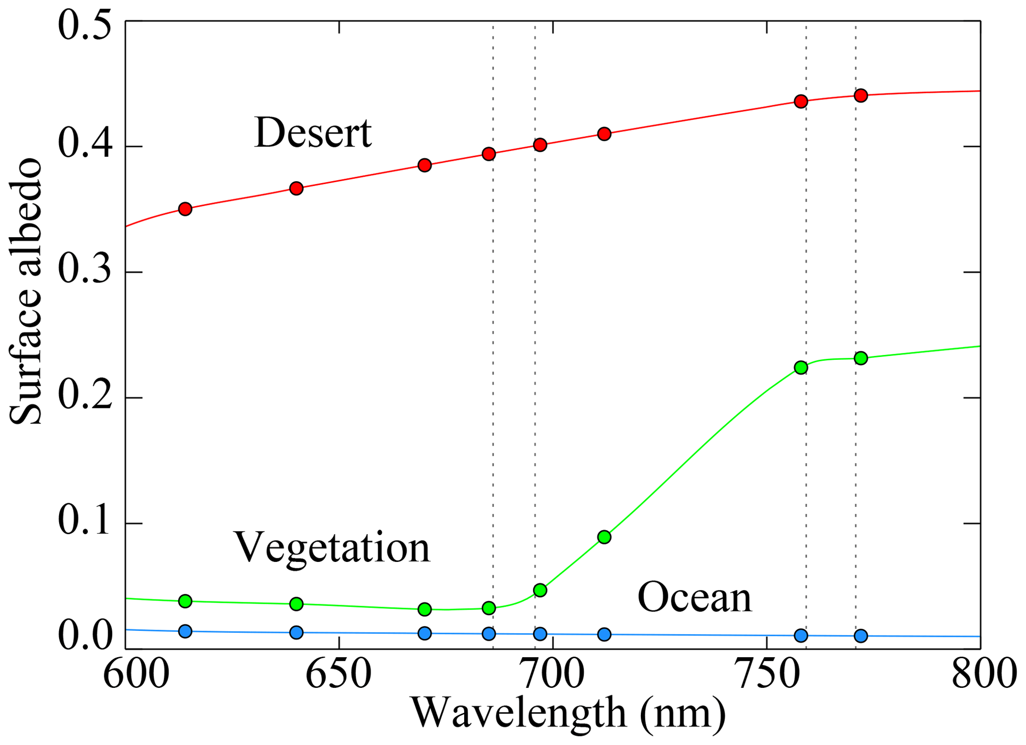
Figure 2Mean surface albedo over 1 month (August) and for different surface types as a function of wavelength. “Desert” stands for the Sahara, “Ocean” for the Atlantic Ocean and “Vegetation” for the Amazon rainforest. The vertical dashed lines indicate the location of the oxygen A band (around 761 nm) and B band (around 687 nm). The values come from the SCIAMACHY surface albedo database described in Tilstra et al. (2017).
3.1 Oxygen A and B bands
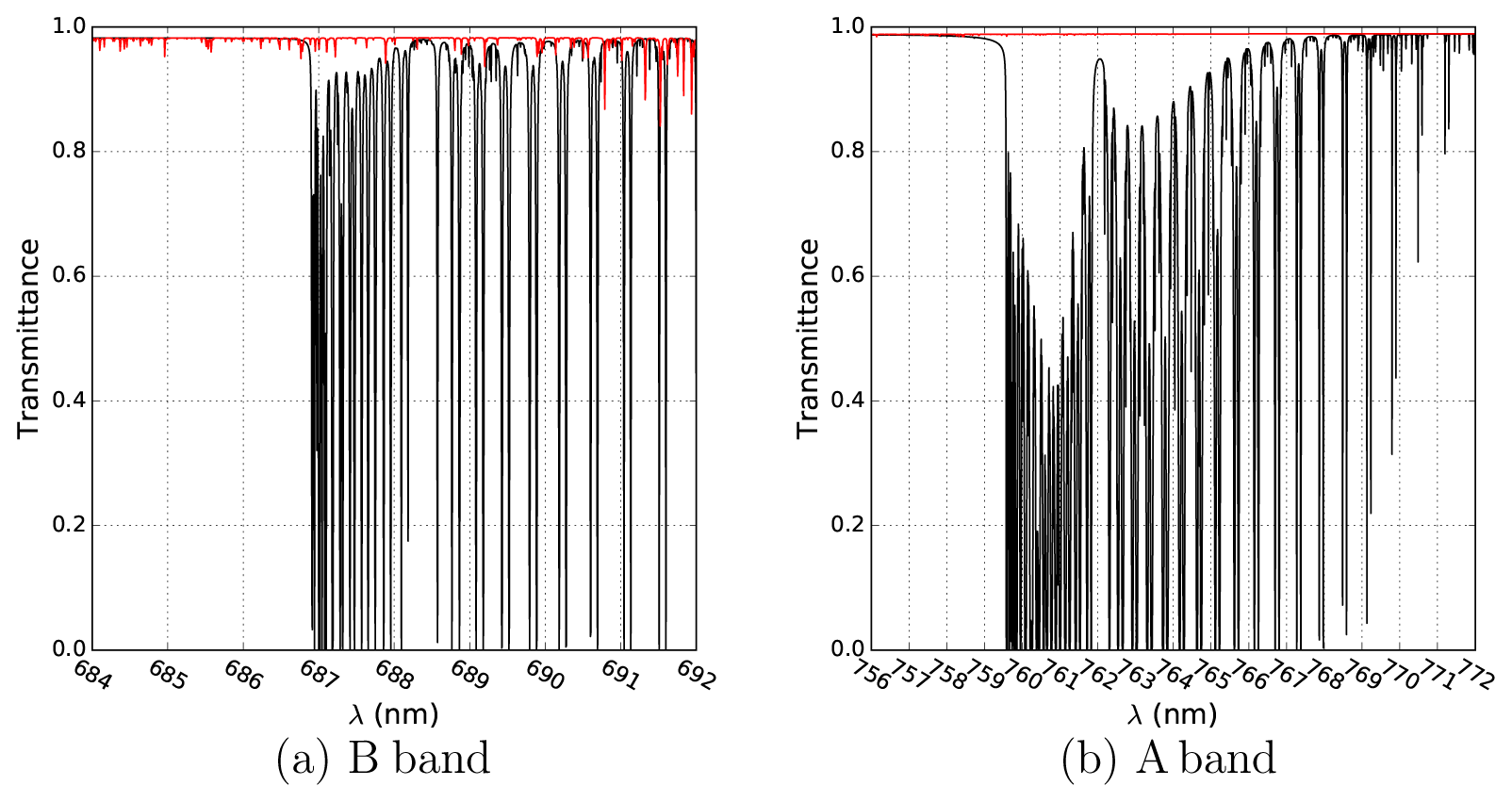
Figure 3Line-by-line transmittances in the oxygen A (b) and B (a) bands (black lines). The transmittances of the overlapping water vapour lines are represented in red. The calculations are computed using the HITRAN2016 database (Gordon et al., 2017) for a solar zenith angle of 0∘.
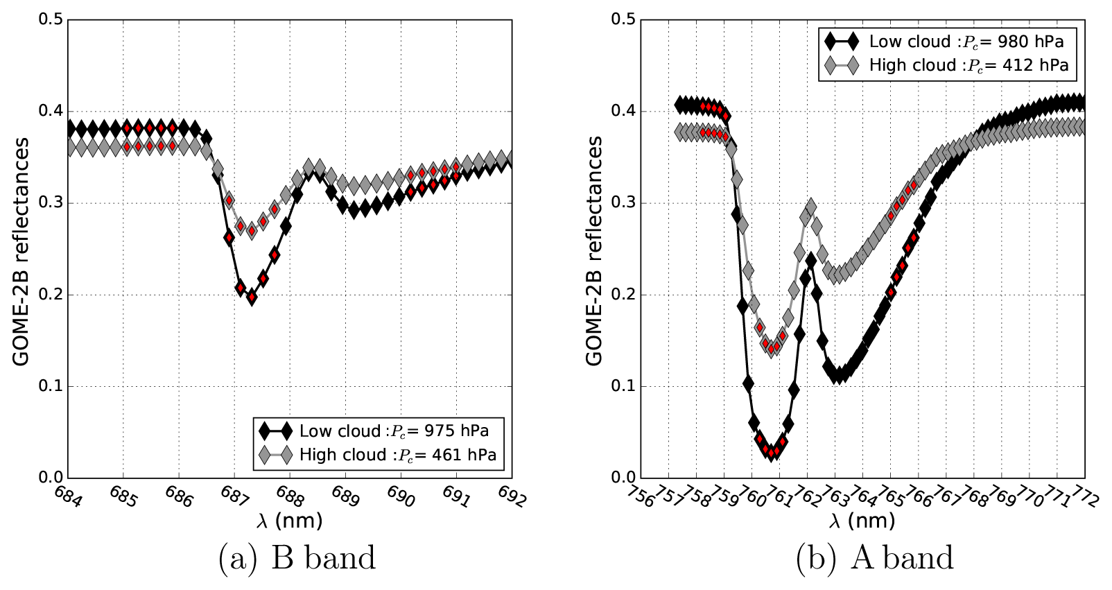
Figure 4Example of GOME-2B spectral reflectance measurements in the B band (a) and A band (b) for low clouds (black line) and high clouds (grey line) taken from a pixel over ocean. The red symbols in (a) and (b) indicate the measurements that are used in the FRESCO-B and FRESCO algorithms, respectively. The cloud pressures retrieved with FRESCO-B and FRESCO are indicated.
The oxygen molecule has two strong absorption bands: the A band around 761 nm and the B band around 687 nm. Figure 3 shows the high-resolution transmittances calculated using the 2016 HITRAN database (Gordon et al., 2017). We can clearly see that the B band is less deep than the A band, which means that less light is absorbed by oxygen in the B band than in the A band. With the hypothesis of a cloud acting like a high-albedo Lambertian reflector, the cloud height retrieved in the B band is usually lower than the cloud height retrieved in the A band (Yang et al., 2013). This is visible in Fig. 4, which shows GOME-2B measurements in the oxygen A and B bands for two clouds at different altitudes over ocean. For the low cloud (black lines), FRESCO-B and FRESCO retrieve similar cloud pressures of 975 and 980 hPa, respectively. However, for the high cloud, the retrieved pressures are quite different, as FRESCO-B cloud pressure is 461 hPa, while FRESCO cloud pressure is 412 hPa. This large difference will be discussed later on, but it is clear that retrieving cloud height from measurements in the oxygen B band is very valuable. Indeed, it brings new information regarding the vertical location of the cloud, which can then be used together with the measurements in the oxygen A band in order to have more information about the cloud layer.
3.2 FRESCO-B retrieval method
Similarly to FRESCO (Koelemeijer et al., 2001; Wang et al., 2008), the FRESCO-B retrieval method is based on minimising the difference between a measured and a simulated spectrum using a Levenberg–Marquardt non-linear least-squares method. FRESCO-B retrieves the effective cloud fraction and the cloud pressure from the top-of-atmosphere reflectances at three 1 nm wide windows: namely 685–686, 686.8–687.8 and 690–691 nm. The wavelengths are chosen in order to maximise the difference in absorption between the windows. Figure 3 also shows that the contamination by water vapour is small so we decided to neglect it. Each of the three windows contains five reflectance measurements by GOME-2B as can be seen in Fig. 4a. While the reflectances measured in the continuum (between 685 and 686 nm) are not impacted by the altitude of the cloud but only by its albedo, the amount of absorption in the two other windows varies according to the cloud altitude.
4.1 Methodology
In order to understand FRESCO-B and its differences with FRESCO, we have simulated spectra for four different cloud cases. O2 A- and B-band reflectance spectra have been simulated with the DAK (Doubling-Adding KNMI) model (De Haan et al., 1987; Stammes et al., 1989; Stammes, 2001), which is a line-by-line radiative transfer model. The spectral simulations have been made for a mid-latitude summer atmosphere consisting of 33 plane-parallel homogeneous layers with multiple scattering and oxygen absorption. The O2 absorption cross sections were calculated using HITRAN2016 line parameters (Gordon et al., 2017). In this atmosphere, homogeneous scattering cloud layers are inserted with varying optical thickness. The cloud particle scattering phase function is a Henyey–Greenstein function with an asymmetry parameter of 0.85 and a single scattering albedo of 1. The cloud scenes are simulated with single-layer clouds, which fully cover the pixels with a top altitude of either 5 or 10 km, a geometrical thickness of 3 km, and an optical thickness of 9 or 42. The four different cases, similar to the ones used in Sneep et al. (2008), are described in Table 1. The spectra were calculated from 684 to 692 nm for the B band and from 756 to 772 nm for the A band, both at 0.005 nm resolution. For each band, the simulations have been done for ocean and vegetation, with surface albedo values taken from the database described in Sect. 2. Following this, we have convolved the obtained spectra with the GOME-2B slit functions and applied the FRESCO-B and FRESCO algorithms. Results are shown for four different viewing and solar geometries.
4.2 Cloud fraction
In Fig. 5, we can see that the retrieved effective cloud fraction is sometimes higher than 1. This is due to the principle of the FRESCO algorithm. Indeed, the effective cloud fraction is the part of the pixel that the Lambertian cloud has to occupy to match the observed reflectance, while the geometric cloud fraction is the part of the pixel that is covered by the true clouds. The effective cloud fraction is strongly coupled to the choice of the cloud albedo Ac. The choice of Ac=0.8 has been made in the FRESCO algorithm (Koelemeijer et al., 2001; Stammes et al., 2008) for various reasons (correction of trace gases for clouds, consistency of the Lambertian model, ability to approach the measured reflectivities by simulations) and can lead to effective cloud fractions somewhat higher than 1.
In Fig. 5a, we can see that, for the cloud cases over ocean, the effective cloud fraction retrieved with FRESCO-B and FRESCO are very similar, as the difference ranges from 0 to 0.02. Figure 5b shows that over vegetation the difference between the two effective cloud fractions is higher as it is comprised between 0.01 and 0.04. The effective cloud fraction retrieved with FRESCO-B is always higher than the one retrieved with FRESCO. This behaviour is as expected. Indeed, for wavelengths in the continuum (which are used in the effective cloud fraction retrievals), we may set T=1 in Eq. (1). Using Rsim(λ)≈Rmeas(λ) leads to the following equation:
Differentiation to As gives the change in the retrieved effective cloud fraction, Δc, due to a small change in the assumed surface albedo, ΔAs (Koelemeijer et al., 2001):
As the albedo of vegetation is lower in the B band than in the A band (see Fig. 2), we expect to retrieve a higher cloud fraction with FRESCO-B for this type of surface. For ocean, the surface albedo chosen for the simulations is the same in the two spectral regions, so we do not expect any impact on the effective cloud fraction.
Table 1Parameters for the four cloud cases used in the retrieval simulations.
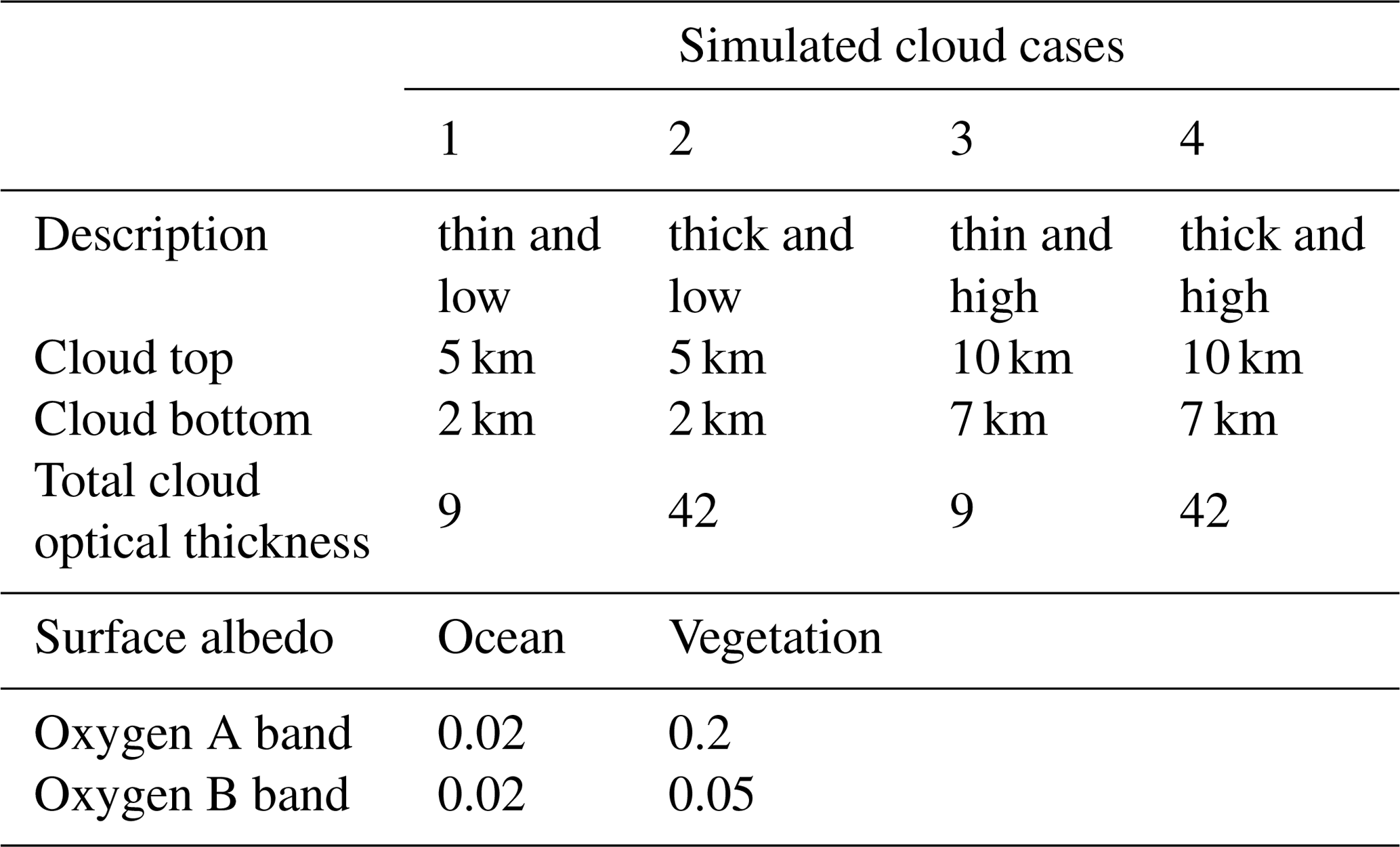
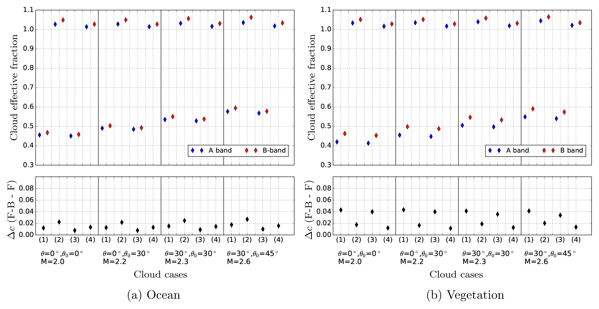
Figure 5FRESCO-B (F-B) and FRESCO (F) effective cloud fraction retrievals (top panels) and effective cloud fraction differences (bottom panels) for the simulated cloud scenes over ocean (a) and vegetation (b). The cloud cases are described in Table 1. The simulations have been made with an azimuth angle difference of 90∘.
4.3 Cloud pressure
In Fig. 6, we see that the pressures retrieved by FRESCO-B and FRESCO in the simulations indicate an altitude inside the cloud layer but well below the cloud top altitude. This feature is well known and common to algorithms which are based upon the hypothesis of a Lambertian cloud to retrieve the cloud top pressure (Saiedy et al., 1965; Vanbauce et al., 1998; Parol et al., 1999; Wang et al., 2008; Sneep et al., 2008). Indeed, real clouds do not act as perfect reflecting boundaries and the algorithm takes into account neither the photons reflected by the surface below the cloud, nor the photon penetration into the cloud layer. In both cases, the photon path increases in addition to the oxygen absorption, which leads to a higher pressure than the cloud top. For optically thick clouds, the retrieved pressure is closer to the cloud top than for thinner clouds; the thick clouds are closer to the model of a Lambertian cloud. We also observe a decrease in the retrieved cloud pressures with increasing geometric air mass factor. Indeed, the larger the solar and viewing zenith angles are, the shallower the photon penetrates into the cloud layer.
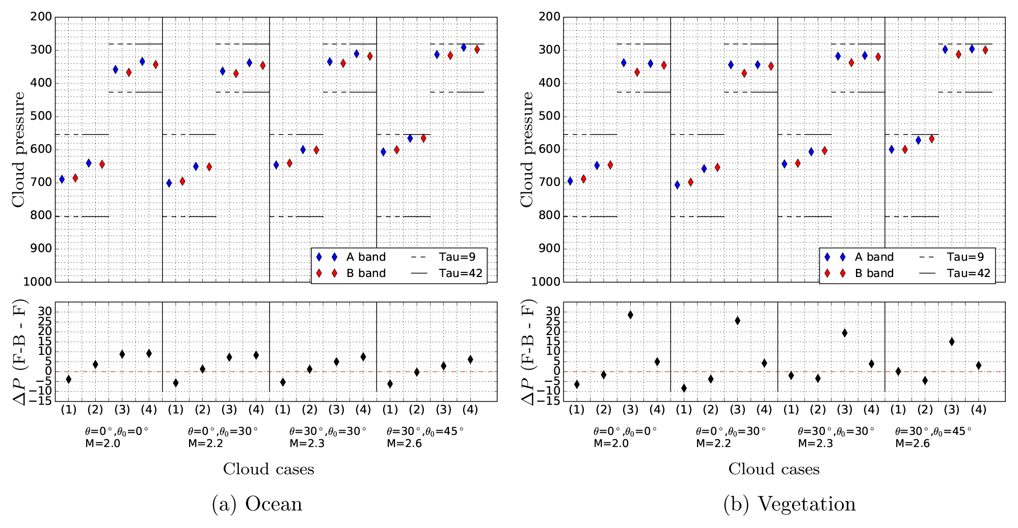
Figure 6FRESCO-B (F-B) and FRESCO (F) cloud pressure retrievals (top panels) and cloud pressure differences (bottom panels) for the simulated cloud scenes over ocean (a) and vegetation (b). The cloud cases are described in Table 1. The simulations have been made with an azimuth angle difference of 90∘.
In Fig. 6a, we can see that, over ocean, the difference in retrieved pressure between FRESCO-B and FRESCO is between about −5 and +10 hPa and increases with the cloud altitude. Indeed, the higher the cloud, the longer the photon's path under the cloud, where it undergoes oxygen absorption. As this path under the cloud is not taken into account in FRESCO and FRESCO-B, high cloud altitudes lead to larger pressure differences.
In Fig. 6b, we can see that over vegetation the difference in pressure between FRESCO-B and FRESCO is between about −10 and +10 hPa, except for high (top altitude 10 km), optically thin clouds (τ=9) clouds, where the difference is much larger. The reason that FRESCO-B retrieves a (much higher) higher cloud pressure than FRESCO for (thin) high clouds is twofold. Firstly, the O2 B band is less strong than the O2 A band so that radiation in the B band penetrates deeper into clouds and the atmosphere than in the A band, thus down to higher pressures. Secondly, for optically thin clouds there is a relatively large cloud-free part of the pixel in the FRESCO retrieval model (see Fig. 1). Since the surface albedo of land is higher in the O2 A band than in the O2 B band, there are more photons reflected by the surface in the A band than in the B band for the cloud-free part. These photons have experienced high pressure and large O2 absorption. To compensate for this large O2 absorption, the FRESCO retrieval places the cloud at a lower pressure than the FRESCO-B retrieval does. Both effects lead to a positive difference between FRESCO-B and FRESCO cloud pressures. The second effect explains the surface albedo bias of the FRESCO retrieval as compared to the FRESCO-B retrieval.
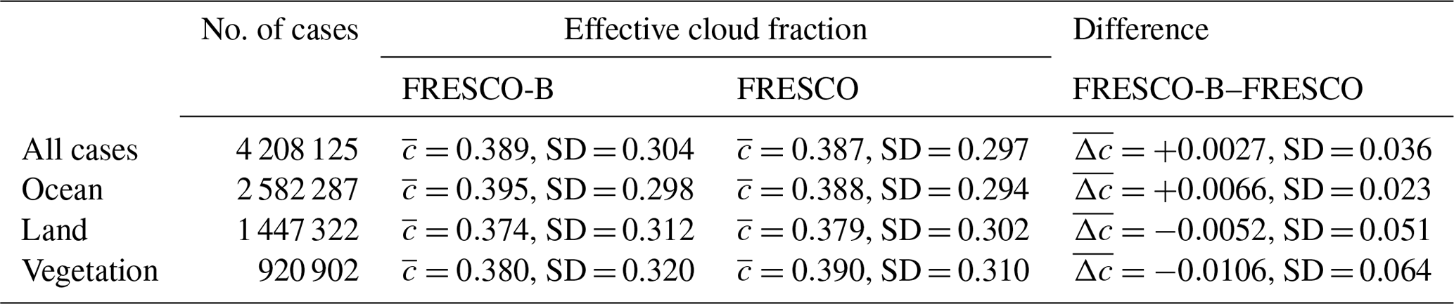
Table 2Mean effective cloud fractions and standard deviations for FRESCO-B and FRESCO, as well as the mean difference between them, for GOME-2B measurements in July 2014 over different surfaces. The vegetation category is a subpart of the land category.
For the case of a low, thin cloud, the FRESCO-B pressure is a bit lower than the FRESCO pressure. This holds for both the ocean and vegetation cases, except for the most oblique geometry for vegetation. This feature can be due to the Rayleigh scattering. Since the B band is weaker than the A band, multiple scattering between the cloud particles and the molecular Rayleigh scatterers above, inside and below the cloud is stronger in the B band than in the A band. At 685 nm there is 50 % more Rayleigh scattering than at 760 nm. Most Rayleigh scattering is above 5 km, so the pressure retrieved in the B band is lowered by the scattering happening above the cloud, leading to a smaller (negative) difference in pressure.
The FRESCO algorithm works best for clouds over a dark surface because in that case the major part of the radiation comes from the cloud and not from the surface. When the surface albedo is increased in FRESCO, which happens when going from the O2 B band to the O2 A band, the cloud fraction and the cloud pressure decreases (the cloud rises). This behaviour agrees with earlier studies, simulations and retrievals of FRESCO using the A band when changing the surface albedo. In our simulations of clouds over vegetation the cloud fraction is indeed decreasing when going from the B band to the A band and the cloud pressure is decreasing for high, thin clouds by about 25–30 hPa when going from the B band to the A band.
5.1 FRESCO in the oxygen A and B bands applied to GOME-2B data
In this section we compare the effective cloud fraction and cloud pressure retrieved by the two versions of FRESCO. We have run the two algorithms over 1 month of GOME-2B data in July 2014, excluding the snow and ice cases. The dataset contains 4 208 125 cases.
5.1.1 Cloud fraction
The differences of effective cloud fraction between FRESCO-B and FRESCO are shown in Fig. 7a. We see the highest difference at high latitudes and over bright surfaces. The distributions of the differences between FRESCO-B and FRESCO retrievals over ocean and land are shown in Fig. 8a and b and the mean values are summarised in Table 2. Both over ocean and land the differences are almost zero, with mean values of +0.0066 and −0.0052, respectively. These very small differences are expected as the cloud fraction is mainly determined through the reflectance measurements performed in the non-absorbed part of the spectrum. Over land, the distribution of the cloud effective fraction differences is more widespread than over ocean, which is due to the more important variability of the surface albedo over this type of surface.
However, over vegetation both Fig. 7a and Table 2 show that the effective cloud fraction retrieved in the B band is lower than the one retrieved in the A band, while the simulations suggest the opposite (see Sect. 4.2). Indeed, although the surface reflectance has an anisotropic BRDF function, the surface is often assumed to be Lambertian, as in many situations the full BRDF is not available or the radiative transfer code used is not equipped to handle the BRDF properly. This is the case in FRESCO and FRESCO-B for which we use a MODE-LER surface albedo climatology established from SCIAMACHY measurements (Tilstra et al., 2017). This anisotropy is stronger over vegetation which has non-isotropic elements like dense trees with heterogeneous leaves and shadow effects and in the near-infrared (NIR) domain (0.7–2.5 µm), where the atmosphere is more transparent. Recently, Lorente et al. (2018) have shown that this assumption of a Lambertian surface leads to across-track biases on satellite retrievals that use those climatologies, such as the effective cloud fraction, for the solar and viewing geometries of GOME-2. It is shown by Lorente et al. (2018) that the western part of the swath has the most biased FRESCO cloud fraction. Consequently, for the vegetation case, we have recompiled the mean effective cloud fractions for FRESCO and FRESCO-B, distinguishing the eastern, nadir and western pixels of the GOME-2B swath. The results are summarised in Table 3. We see that for the eastern and nadir pixels of the swath, the effective cloud fraction retrieved by FRESCO-B is higher than the one retrieved by FRESCO, which agrees with our simulations, while for the western pixels this is the opposite. Indeed, for the western part of the swath, the cloud effective fraction retrieved in the O2 A band is too high because the surface albedo is high (red edge; Tilstra et al., 2017) and the anisotropy is stronger, while in the O2 B band the surface albedo is low and the anisotropy is smaller. Consequently, the error in As due to the assumption of a Lambertian surface has a smaller impact on effective cloud fraction in the B band than in the A band. This difference in behaviour of the retrievals according to the part of the swath corroborates the conclusions of Lorente et al. (2018).
Table 3Mean effective cloud fractions and standard deviations for FRESCO-B and FRESCO, as well as the mean difference, for GOME-2B measurements in July 2014 over vegetation. We distinguish the eastern (pixels 1 to 8), nadir (pixels 9 to 16) and western (pixels 17 to 24) parts of the swath.
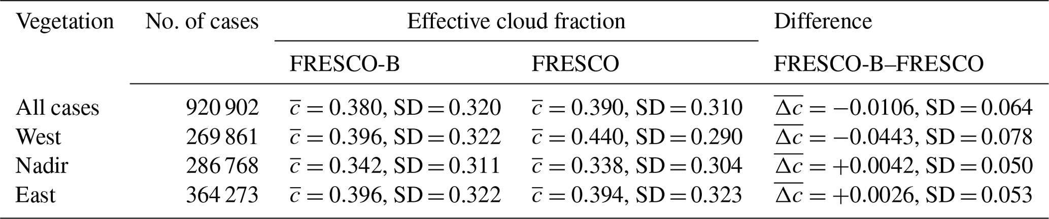
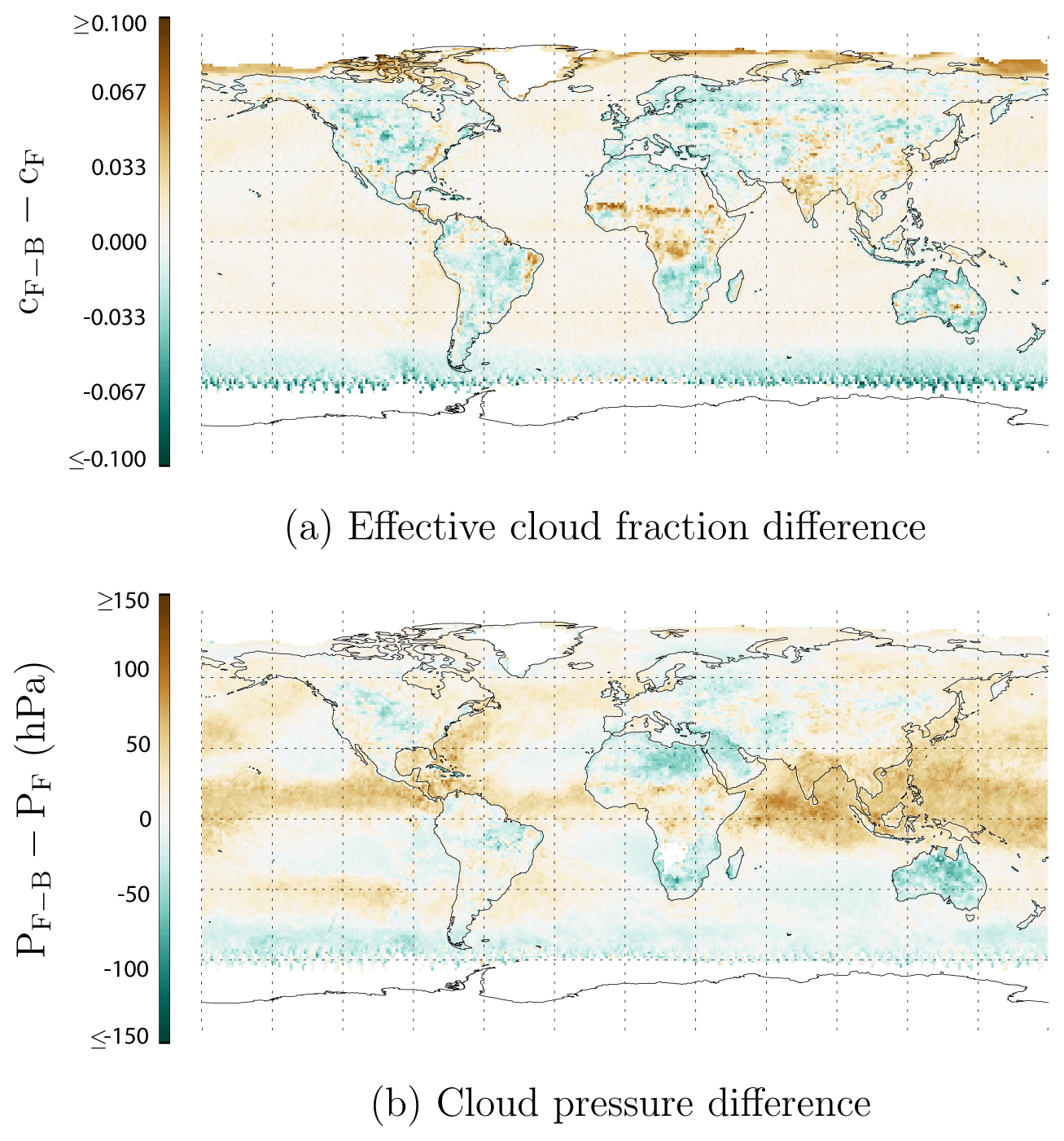
Figure 7Differences of effective cloud fraction and cloud pressure between FRESCO-B and FRESCO for July 2014.
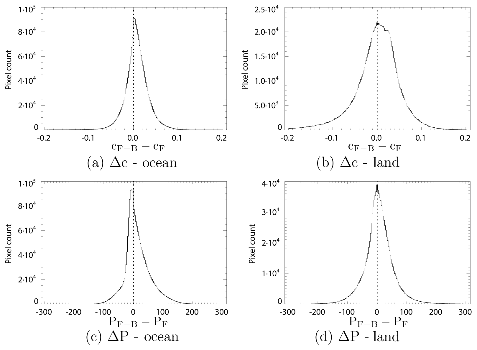
Figure 8Histograms of the differences in effective cloud fraction (a, b) and cloud pressure (c, d) between FRESCO-B and FRESCO for July 2014 over ocean (a, c) and over land (b, d).
5.1.2 Cloud pressure
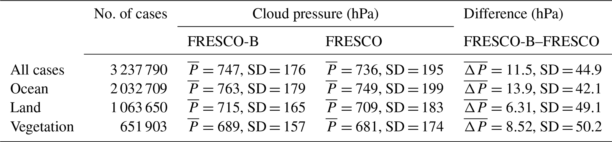
Table 4Mean cloud pressures and standard deviations for FRESCO-B and FRESCO, as well as the mean difference between FRESCO-B and FRESCO, for GOME-2B measurements in July 2014 over different surfaces. The vegetation category is a subpart of the land category.
In this subsection we limit our study to the pixels for which the FRESCO effective cloud fraction is higher than or equal to 0.1; indeed, as mentioned in Wang et al. (2008), cloud pressures have large uncertainties when effective cloud fraction is lower than 0.1. This selection leaves us with 3 237 790 pixels.
The differences in cloud pressure retrieved with FRESCO-B and FRESCO are shown in Fig. 7b. We have also analysed the differences separating the pixels according to the underlying surface type. The distributions of the differences between FRESCO-B and FRESCO are shown in Fig. 8c and d, while the mean values are summarised in Table 4. The mean cloud pressures are 736±195 hPa in the A band and 747±176 hPa in the B band. As already mentioned, this behaviour is expected as the B band is less absorbing.

Figure 9MODIS normalised difference vegetation index (NDVI) for July 2014. Source: https://earthobservatory.nasa.gov/global-maps/TRMM_3B43M/MOD_NDVI_M (last access: 2 April 2019)
Over ocean the mean cloud pressure is 763±179 hPa with FRESCO-B, while with FRESCO this value is 749±199 hPa and the mean difference is 13.9±42.1 hPa. The surface albedo of ocean is very similar in the oxygen A and B bands; therefore, the differences we observe in cloud pressure are only due to a difference in absorption inside and under the cloud. For instance, in Fig. 7b, we observe the larger pressure differences in the intertropical convergence zone (ITCZ), where there are a lot of high clouds (cumulonimbus, cirrus), which agrees with the simulations presented in Sect. 4.3. Over ocean, the coefficient of correlation between the difference in pressure and the difference in cloud effective fraction is 0.0949.
Over land, the cloud pressure difference is also positive on average, with a mean value of 6.31±49.1 hPa. However, as we can see in Fig. 8d, the range of the values is larger than over ocean, with a lot of pixels having a negative difference in pressure. This is again due to the high variability of the surface albedo for this type of surface and is coherent with the observations we have made of the simulations. Over land, the coefficient of correlation between the difference in pressure and the difference in cloud effective fractions is 0.523.
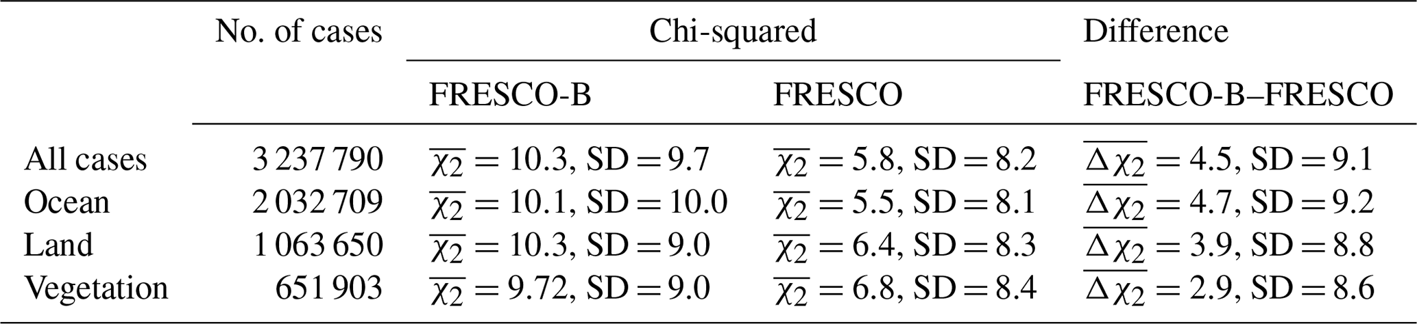
Over vegetation, we observe small pressure differences on average, the mean cloud pressures being 689±157 hPa with FRESCO-B and 681±174 hPa with FRESCO. Figure 9 allows us to visualise the vegetated areas in July (the higher the index, the greener the area). We can see in Fig. 7b that those areas (north-western North America, northern South America and the northern part of Europe and Asia have, on average, small cloud pressure differences, which also agrees with the simulations we have described in Sect. 4.3. Moreover, as seen in Fig. 2, the surface albedo of vegetation surfaces is much lower in the oxygen B band than in the oxygen A band. Therefore, the contribution of the ground in the reflectances is lower in the oxygen B band than in the A band, so we expect more accurate retrievals in the B band. Table 5 shows the value of χ2 obtained with FRESCO and FRESCO-B for different types of surfaces. We can see that the χ2 is always higher for FRESCO-B than FRESCO. This is due to the fits of the algorithms: the difference between the simulated reflectances and the measured ones is always higher in the B band. However, we can notice that while with FRESCO the χ2 is higher for vegetation, this is the opposite with FRESCO-B. FRESCO-B is the most suited over vegetated surfaces.
Table 5Mean chi-squared and standard deviations for FRESCO-B and FRESCO, as well as the mean difference between FRESCO-B and FRESCO, for GOME-2B measurements in July 2014 over different surfaces. The vegetation category is a subpart of the land category.
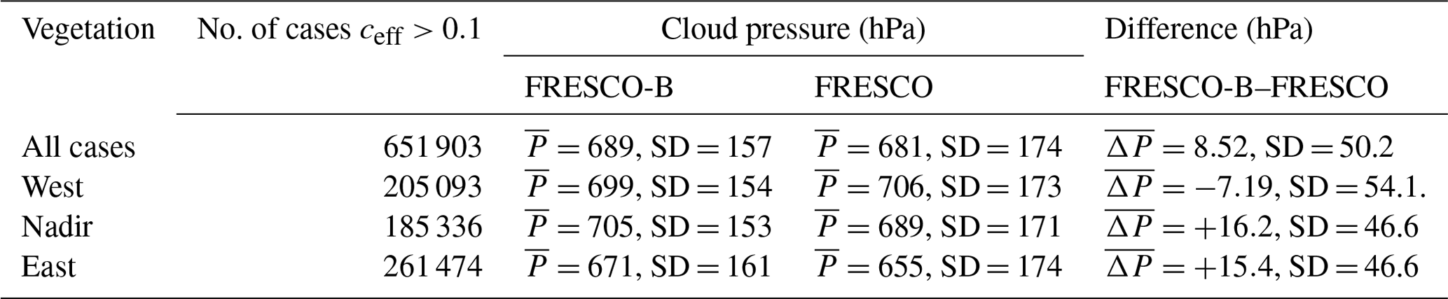
As we have mentioned the anisotropy of the surface albedo over vegetation and its consequences on effective cloud fraction retrieval previously, we have compiled the mean cloud pressure retrieved with FRESCO and FRESCO-B for the different part of the swath. The results are summarised in Table 6. We see that the pressure retrieved with FRESCO-B is higher than the one retrieved with FRESCO for the eastern and nadir part of the swath, while it is the opposite for the western pixels. This last observation is due to the bias albedo on the western part of the swath: as mentioned in Sect. 5.1.1, the use of a Lambertian albedo in FRESCO and FRESCO-B leads to artificially high values of FRESCO effective cloud fraction for those pixels and consequently to artificially low values of FRESCO cloud pressure (see Eq. 1). On the other side, the B band is less impacted by the bias albedo as is the FRESCO-B cloud pressure. This albedo bias impacting more of the O2 A-band measurements than the O2 B band leads to a higher cloud pressure difference than expected.
Table 6Mean cloud pressure for FRESCO-B and FRESCO, as well as the difference between them, for GOME-2B measurements in July 2014 over vegetation. We distinguish the eastern (pixels 1 to 8), nadir (pixels 9 to 16) and western (pixels 17 to 24) parts of the swath .
The mean difference in cloud pressure between FRESCO-B and FRESCO is 11.5 hPa, but the difference does not have the same signification according to the underlying surface: over ocean, the two pressures indicate different pieces of information about the vertical structure of the cloud layer, while over vegetation the difference is partly due to the difference in surface albedo. Over vegetation, the FRESCO-B cloud pressure is more accurate than the FRESCO one. In the future we also recommend using a surface albedo database which takes into account the anisotropy of the surface to avoid biases.
5.2 Comparison with ground-based measurements
5.2.1 Cloudnet target classification product
Cloudnet is a network of ground-based measurement facilities for the evaluation of clouds and aerosols in forecast models. Cloudnet started around 2001 with three observation sites (at Cabauw, Palaiseau and Chilbolton) and includes now five other permanent sites (at Jülich, Leipzig, Lindenberg, Mace Head and Potenza). In this study, we reject the data from the Mace Head site as it is on the seaside, while the other sites can be considered to be surrounded by vegetation. These sites are equipped with active sensors, such as lidar and Doppler millimetre-wave radar that provide vertical profiles of cloud and aerosol properties, as well as ice and liquid cloud water content, at high temporal and spatial resolution. In this study, we use the Cloudnet level 2 classification product (Illingworth et al., 2007), which is based on the combination of the vertically pointing Doppler cloud radar and backscatter lidar and is available approximately every 30 s. This product classifies each vertical layer as 1 of 11 classes, which distinguishes ice and water clouds, precipitation, aerosols, insects, clear sky, and combination thereof. Indeed the radar detects large particles such as rain and drizzle drops, ice particles and insects, while the lidar is sensitive to smaller particles such as cloud droplets and aerosols. The target classification product also contains cloud top height and cloud base height. Cloud top and cloud base heights correspond, respectively, to the highest and lowest altitudes of the backscatter altitude grid boxes that have clouds. Consequently, for multilayer cloud situations, the cloud top height refers to the top of the highest layer, while the cloud base height refers to the base of the lowest layer.
5.2.2 Methodology
In this section we perform comparisons between the two versions of the FRESCO and Cloudnet target classification products and the cloud boundaries for the seven Cloudnet observation sites in July and August 2014. For every GOME-2B pixel collocated with a Cloudnet site, we select 1 h (±30 min) of Cloudnet target classification. For every cloud height measurement from GOME-2B, there are about 120 (temporal) × 495 (vertical) radar and lidar backscatter Cloudnet pixels, which are classified as 1 of the 11 categories mentioned earlier. In this study, we keep the cloudy cases, which consist of the classes “ice” and “cloud droplets only” as well as the precipitation classes: “drizzle or rain”, “drizzle or rain and cloud droplets”, “ice and supercooled droplets”, “melting ice”, and “melting ice and cloud droplets”. We then determine the height distributions of the backscatter pixels, from 270 to 15 000 m with a bin size of 270 m, following the method defined by Wang and Stammes (2014). If the distribution presents a unique mode, without an interruption by a clear-sky pixel, the cloud is considered a monolayer case. If not, it is classified as a multilayer case. The Cloudnet cloud top and base heights are calculated averaging the cloud top and base heights in the 1 h period around the GOME-2B overpass time.
5.2.3 Results
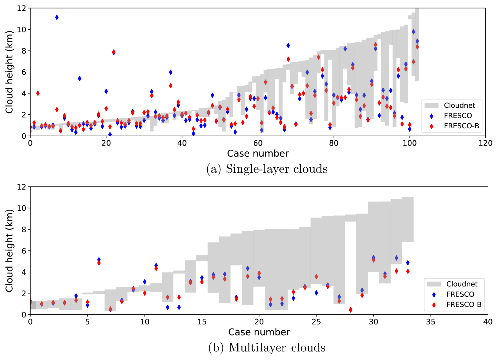
Figure 10Comparison of the cloud heights retrieved by FRESCO-B, FRESCO and Cloudnet in July and August 2014 for six Cloudnet sites (Hyytiälä, Jülich, Leipzig, Lindenberg, Palaiseau and Potenza).
For the 2 months considered, the collocation process provides us with 339 collocated cloud cases that we further filter as follows.
-
We keep only the cases for which the Cloudnet cloud fraction is higher than 0.05. This Cloudnet cloud fraction is calculated by dividing the number of cloudy pixels by the number of pixels accumulated during the 1 h period. With this filtering, we exclude the almost cloud-free scenes.
-
Then we further filter the Cloudnet data excluding the cases for which the standard deviation of the cloud top height exceeds 1.5 km. This criterion used in Veefkind et al. (2016) allows us to avoid the cases with a large temporal variability during the satellite overpass.
-
Finally, we filter the cases according to the FRESCO-B cloud fraction, excluding the cases with c<0.1. Indeed, it is known that the FRESCO cloud pressures are often too low when the cloud fraction is lower than 0.1 (Wang et al., 2008).
Those criteria leave us with 138 cases: monolayer clouds are represented in Fig. 10a, while multilayer situations are shown in Fig. 10b. In both panels, the clouds are ordered by increasing Cloudnet top height altitude. We can distinguish three different regimes, for which the clouds properties are resumed in Table 7.
-
For 68 cases (49 % of the clouds), the FRESCO-B cloud pressure is inside the Cloudnet cloud boundaries. This population corresponds to 46 % of the monolayer clouds and to 59 % of the multilayer clouds and concerns vertically extended middle to high clouds (mean cloud height of 5.5 km and mean cloud thickness of 3.7 km). With FRESCO, the retrieved pressure is inside the Cloudnet boundaries for 64 cases (46 % of the clouds) that are a bit higher (mean altitude of 6 km) and a bit thicker (mean thickness 4.1 km) than for FRESCO-B.
-
In 51 cases, the FRESCO-B cloud pressure indicates an altitude lower than the Cloudnet cloud boundaries. This expected behaviour concerns mainly middle to high (mean cloud height of 5.7 km) monolayer clouds with a limited vertical extent (mean geometrical thickness of 2 km). As already shown (Wang et al., 2008; Sneep et al., 2008), light can penetrate within the clouds where it is absorbed. As this phenomenon is not taken into account in FRESCO, the retrieved cloud height is lower than the cloud top height. This is the case in other retrieval algorithms based on oxygen absorption (Ferlay et al., 2010; Desmons et al., 2013). FRESCO cloud altitude is lower than Cloudnet in 53 cases. It concerns lower (mean altitude of 5.1 km) and thinner (mean thickness of 1.6 km) clouds than for FRESCO-B.
-
In the last 19 cases, the FRESCO-B cloud pressure indicates an altitude higher than the Cloudnet cloud boundaries. This concerns mainly monolayer low (mean top height of 1.9 km) thin (mean cloud geometrical thickness of 0.4 km) clouds. In those cases, many photons are transmitted and reach the surface before being reflected back to space. This situation concerns 21 cases for FRESCO, also quite low (mean top height of 2.3 km) and thin (mean cloud geometrical thickness of 0.5 km).
Table 7Number of collocated cloud cases for which FRESCO-B and FRESCO cloud pressures are inside, lower or higher than the Cloudnet (CN) cloud range. For each case, the mean Cloudnet cloud altitude () and geometrical thickness () are indicated. Collocated Cloudnet–GOME-2B data for July and August 2014 from the Cloudnet sites of Hyytiälä, Jülich, Leipzig, Lindenberg, Palaiseau and Potenza.
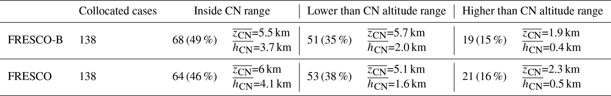
The results shown by FRESCO-B are very similar to the ones obtained with FRESCO; however, FRESCO-B performs slightly better than FRESCO, as with FRESCO-B 49 % of the retrieved cloud pressures are within the Cloudnet cloud boundaries, while this number is 46 % with FRESCO. Additionally, for monolayer clouds, FRESCO-B retrieves an altitude within Cloudnet range in 46 % of the cases, while this value is 41 % with FRESCO. For multilayer clouds, FRESCO performs slightly better than FRESCO-B, indicating an altitude within Cloudnet range for 62 % of the cases, while this value is 59 % with FRESCO-B. Those performances are very promising and show that it would be very valuable to use both FRESCO-B and FRESCO retrievals, particularly in the case of multilayer clouds.
Like in the previous section, we have also filtered the pixels according to their position in the swath, keeping only the nadir and eastern pixels of the swath. Because of this, the FRESCO-B cloud pressure is inside the Cloudnet cloud boundaries in 49 % of the cases, as with all the pixels; for FRESCO, this number stays stable too, as it is now 47 % (46 % for all the swath). Excluding the western pixels of the swath does not seem to change the performance of the two algorithms. However, the size of the database is too small to deduce strong conclusions. We should also keep in mind that the Cloudnet sites are situated in Europe, while the study made by Lorente et al. (2018) takes place in Amazonia. The vegetation is probably very different between those two regions (grass and forests) and their surface albedos are probably different as well.
In this paper, we present a new cloud retrieval algorithm called FRESCO-B for GOME-2 measurements in the oxygen B band. FRESCO-B is based on the algorithm FRESCO, which uses measurements in the oxygen A band to retrieve cloud properties (effective cloud fraction and cloud pressure). However, while the surface albedo in the O2 A band is very low over ocean, the albedo takes larger values over vegetation, which can lead to biases in the retrievals. In this paper, we apply FRESCO-B to GOME-2B measurements in the O2 B band, which is a wavelength range where the surface albedo stays relatively low whatever the underlying surface is.
First, we simulated cloudy scenes, which showed that FRESCO-B and FRESCO retrievals indicate an altitude inside the cloud layer but well below the top, which was expected. We have noted that the difference between the pressures obtained with the two algorithms depends on the geometry of the scenes and ranges between −10 and +10 hPa, except for high, thin clouds where it can reach +30 hPa. Then inter-comparisons between FRESCO-B and FRESCO over 1 month of GOME-2B data showed that the effective cloud fraction retrieved is very similar in the two bands. These comparisons have also revealed that FRESCO-B retrieves a higher cloud pressure than FRESCO (mean difference of 11.5 hPa) and is more accurate over vegetation (χ2 is lower over vegetation than for other surfaces). Finally, we have validated FRESCO-B and FRESCO to in situ data over vegetation obtained with the Cloudnet network of instruments. These comparisons have shown that FRESCO-B and FRESCO can retrieve a pressure which stands inside the cloud layers for clouds that are not too far from the Lambertian model. In the future, we would like to apply FRESCO-B and FRESCO to TROPOMI (Veefkind et al., 2012) measurements in the O2 A and B bands. Indeed its high spatial resolution (7 km × 3.5 km) compared to previous spectrometers (80 km × 40 km for GOME-2B) should provide much more detailed cloud structures.
In the future, the authors would like to merge the measurements in the O2 A and B bands in order to retrieve more information about the vertical structure of cloud layers. Excluding the western part of the swath of GOME-2B in the comparisons has improved the performance of FRESCO-B, which corroborates the conclusions of Lorente et al. (2018) on the surface albedo bias regarding these pixels. Since this bias leads to biases in cloud retrievals, the authors recommend taking into account the anisotropy of the surface reflectances for future surface albedo climatologies (ongoing work within within the Eumetsat satellite application facility on atmospheric composition monitoring project).
As FRESCO-B is not operational yet, the data is available per request.
The authors declare that they have no conflict of interest.
This research was funded by the Netherlands Space Office (NSO) User Support Programme Space Research through the FRESCO-B project, ALW-GO/16-23. We acknowledge the EU Cloudnet and the EU H2020 ACTRIS projects for providing the cloud classification datasets for the Cloudnet sites. We thank Maarten Sneep and Olaf Tuinder for the processing and visualisation tools they have provided.
This paper was edited by Jun Wang and reviewed by two anonymous referees.
Andrews, T., Gregory, J., Webb, M. J., and Taylor, K. E.: Forcing, feedbacks and climate sensitivity in CMIP5 coupled atmosphere-ocean climate models, Geophys. Res. Lett., 39, L09712, https://doi.org/10.1029/2012GL051607, 2012. a
Boersma, K. F., Eskes, H. J., and Brinksma, E. J.: Error analysis for tropospheric NO2 retrieval from space, J. Geophys. Res., 109, D04311, https://doi.org/10.1029/2003JD003962, 2004. a
Bony, S. and Dufresne, J.-L.: Marine boundary layer clouds at the heart of tropical cloud feedback uncertainties in climate models, Geophys. Res. Lett., 32, L20806, https://doi.org/10.1029/2005GL023851, 2005. a
De Haan, J. F., Bosma, P. B, and Hovenier, J. W.: The adding method for multiple scattering calculations of polarized light, Astron. Astrophys., 183, 371–391, 1987. a
Desmons, M., Ferlay, N., Parol, F., Mcharek, L., and Vanbauce, C.: Improved information about the vertical location and extent of monolayer clouds from POLDER3 measurements in the oxygen A-band, Atmos. Meas. Tech., 6, 2221–2238, https://doi.org/10.5194/amt-6-2221-2013, 2013. a
Ferlay, N., Thieuleux, F., Cornet, C., Davis, A. B., Dubuisson, P., Ducos, F., Parol, F., Riédi, J., and Vanbauce, C.: Toward New Inferences about Cloud Structures from Multidirectional Measurements in the Oxygen A Band: Middle-of-Cloud Pressure and Cloud Geometrical Thickness from POLDER-3/PARASOL, J. Appl. Meteor. Climatol., 49, 2492–2507, https://doi.org/10.1175/2010JAMC2550.1, 2010. a
Fournier, N., Stammes, P., de Graaf, M., van der A, R., Piters, A., Grzegorski, M., and Kokhanovsky, A.: Improving cloud information over deserts from SCIAMACHY Oxygen A-band measurements, Atmos. Chem. Phys., 6, 163–172, https://doi.org/10.5194/acp-6-163-2006, 2006. a
Gordon, I., Rothman, L., Hill, C., Kochanov, R., Tan, Y., Bernath, P., Birk, M., Boudon, V., Campargue, A., Chance, K., Drouin, B., Flaud, J.-M., Gamache, R., Hodges, J., Jacquemart, D., Perevalov, V., Perrin, A., Shine, K., Smith, M.-A., Tennyson, J., Toon, G., Tran, H., Tyuterev, V., Barbe, A., Császár, A. A., Devi, V., Furtenbacher, T., Harrison, J., Hartmann, J.-M., Jolly, A., Johnson, T., Karman, T., Kleiner, I., Kyuberis, A., Loos, J., Lyulin, O., Massie, S., Mikhailenko, S., Moazzen-Ahmadi, N., Müller, H., Naumenko, O., Nikitin, A., Polyansky, O., Rey, M., Rotger, M., Sharpe, S., Sung, K., Starikova, E., Tashkun, S., Auwera, J. V., Wagner, G., Wilzewski, J., Wcisło, P., Yu, S., and Zak, E.: The HITRAN 2016 molecular spectroscopic database, J. Quant. Spectrosc. Ra., 203, 3–69, https://doi.org/10.1016/j.jqsrt.2017.06.038, 2017. a, b, c, d
Illingworth, A. J., Hogan, R. J., O'Connor, E. J., Bouniol, D., Delanoë, J., Pelon, J., Protat, A., Brooks, M. E., Gaussiat, N., Wilson, D. R., Donovan, D. P., Baltink, H. K., van Zadelhoff, G.-J., Eastment, J. D., Goddard, J. W. F., Wrench, C. L., Haeffelin, M., Krasnov, O. A., Russchenberg, H. W. J., Piriou, J.-M., Vinit, F., Seifert, A., Tompkins, A. M., and Willén, U.: CLOUDNET – Continuous evaluation of Cloud Profiles in Seven Operational Models using Ground-Based Observations, Bull. Amer. Meteor. Soc., 88, 883–898, https://doi.org/10.1175/BAMS-88-6-883, 2007. a
Koelemeijer, R. B. A., Stammes, P., Hovenier, J. W., and de Haan, J. F.: A fast method for retrieval of cloud parameters using Oxygen A band measurements from GOME, J. Geophys. Res., 106, 3475–3490, https://doi.org/10.1029/2000JD900657, 2001. a, b, c, d
Kuze, A. and Chance, K. V.: Analysis of cloud top height and cloud coverage from satellites using the O2 A and B bands, J. Geophys. Res., 99, 14481–14492, https://doi.org/10.1029/94JD01152, 1994. a
Lelli, L., Kokhanovsky, A. A., Rozanov, V. V., Vountas, M., Sayer, A. M., and Burrows, J. P.: Seven years of global retrieval of cloud properties using space-borne data of GOME, Atmos. Meas. Tech., 5, 1551–1570, https://doi.org/10.5194/amt-5-1551-2012, 2012. a
Lindstrot, R., Preusker, R., Ruhtz, T., Heese, B., Wiegner, M., Lindemann, C., and Fischer, J.: Validation of MERIS cloud top pressure using airborne lidar measurements, J. Appl. Meteor. Clim., 45, 1612–1621, https://doi.org/10.1175/JAM2436.1, 2006. a
Lorente, A., Boersma, K. F., Stammes, P., Tilstra, L. G., Richter, A., Yu, H., Kharbouche, S., and Muller, J.-P.: The importance of surface reflectance anisotropy for cloud and NO2 retrievals from GOME-2 and OMI, Atmos. Meas. Tech., 11, 4509–4529, https://doi.org/10.5194/amt-11-4509-2018, 2018. a, b, c, d, e
Marshak, A. and Knyazikhin, Y.: The spectral invariant approximation within canopy radiative transfer to support the use of the EPIC/DSCOVR oxygen B-band for monitoring vegetation, J. Quant. Spectrosc. Ra., 191, 7–12, https://doi.org/10.1016/j.jqsrt.2017.01.015, 2017. a
Parol, F., Buriez, J.-C., Vanbauce, C., Couvert, P., Séze, G., Goloub, P., and Cheinet, S.: First results of the POLDER Earth Radiation Budget and Clouds operational algorithm, IEEE T. Geosci. Remote, 37, 1597–1612, 1999. a
Preusker, R., Fischer, J. P. A., Bennartz, R., and Schüller, L.: Cloud-top pressure retrieval using the oxygen A-band in the IRS-3 MOS intrument, Int. J. Remote. Sens., 28, 1957–1967, https://doi.org/10.1080/01431160600641632, 2007. a
Saiedy, F., Hilleary, D. T., and Morgan, W. A.: Cloud-top altitude measurements from satellites, Appl. Opt., 4, 495–500, 1965. a
Sneep, M., de Haan, J. F., Stammes, P., Wang, P., Vanbauce, C., Vasilkov, A. P., and Levelt, P. F.: Three-way comparison between OMI and PARASOL cloud pressure products, J. Geophys. Res., 113, D15S23, https://doi.org/10.1029/2007JD008694, 2008. a, b, c
Stammes, P.: Satellite Radiance Modelling in the UV-Visible Range, in: Current Problems in Atmospheric Radiation, edited by Smith, W. and Timofeyev, Y., 385–388, A. Deepak, Hampton, VA, 2001. a
Stammes, P., de Haan, J. F., and Hovenier, J. W.: The polarized internal radiation field of a planetary atmosphere, Astron. Astrophys., 225, 239–259, 1989. a
Stammes, P., Sneep, M., de Haan, J. F., Veefkind, J. P., Wang, P., and Levelt, P. F.: Effective cloud fractions from the Ozone Monitoring Instrument: Theoretical framework and validation, J. Geophys. Res.-Atmos., 113, D16S38, https://doi.org/10.1029/2007JD008820, 2008. a
Tilstra, L. G., Tuinder, O. N. E., Wang, P., and Stammes, P.: Surface reflectivity climatologies from UV to NIR determined from Earth observations by GOME-2 and SCIAMACHY, J. Geophys. Res.-Atmos., 122, 4084–4111, https://doi.org/10.1002/2016JD025940, 2017. a, b, c, d, e, f
Vanbauce, C., Buriez, J., Parol, F., Bonnel, B., Sèze, G., and Couvert, P.: Apparent pressure derived from ADEOS-POLDER observations in the oxygen A-band over ocean, Geophys. Res. Lett., 25, 3159–3162, 1998. a, b
Veefkind, J. P., Aben, I., McMullan, K., Föster, H., de Vries, J., Otter, G., Claas, J., Eskes, H. J., de Haan, J. F., Kleipool, Q., van Weele, M., Hasekamp, O., Hoogeveen, R., Landgraf, J., Snel, R., Tol, P., Ingmann, P., Voors, R., Kruizinga, B., Vink, R., Visser, H., and Levelt, P. F.: TROPOMI on the ESA Sentinel-5 Precursor: A GMES mission for global observations of the atmospheric composition for climate, air quality and ozone layer applications, Remote. Sens. Environ., 120, 70–83, https://doi.org/10.1016/j.rse.2011.09.027, 2012. a
Veefkind, J. P., de Haan, J. F., Sneep, M., and Levelt, P. F.: Improvements to the OMI O2-O2 operational cloud algorithm and comparisons with ground-based radar-lidar observations, Atmos. Meas. Tech., 9, 6035–6049, https://doi.org/10.5194/amt-9-6035-2016, 2016. a
Vial, J., Dufresne, J.-L., and Bony, S.: On the interpretation of inter-model spread in CMIP5 climate sensitivity estimates, Clim. Dynam., 41, 3339–3362, https://doi.org/10.1007/s00382-013-1725-9, 2013. a
Wang, P. and Stammes, P.: Evaluation of SCIAMACHY Oxygen A band cloud heights using Cloudnet measurements, Atmos. Meas. Tech., 7, 1331–1350, https://doi.org/10.5194/amt-7-1331-2014, 2014. a, b
Wang, P., Stammes, P., van der A, R., Pinardi, G., and van Roozendael, M.: FRESCO+: an improved O2 A-band cloud retrieval algorithm for tropospheric trace gas retrievals, Atmos. Chem. Phys., 8, 6565–6576, https://doi.org/10.5194/acp-8-6565-2008, 2008. a, b, c, d, e, f, g
Xu, X., Wang, J., Wang, Y., Zeng, J., Torres, O., Yang, Y., Marshak, A., Reid, J., and Miller, S.: Passive remote sensing of altitude and optical depth of dust plumes using the oxygen A and B bands: First results from EPIC/DSCOVR at Lagrange-1 point, Geophys. Res. Lett., 44, 7544–7554, https://doi.org/10.1002/2017GL073939, 2017. a
Yang, Y., Marshak, A., Mao, J., Lyapustin, A., and Herman, J.: A method of retrieving cloud top height and cloud geometrical thickness with oxygen A and B bands for the Deep Space Climate Observatory (DSCOVR) mission: Radiative transfer simulations, J. Quant. Spectrosc. Ra., 122, 141–149, https://doi.org/10.1016/j.jqsrt.2012.09.017, 2013. a, b