the Creative Commons Attribution 4.0 License.
the Creative Commons Attribution 4.0 License.
 | 15 Jan 2019
Implementation of polarization diversity pulse-pair technique using airborne W-band radar
Mengistu Wolde
Alessandro Battaglia
Cuong Nguyen
Andrew L. Pazmany
Anthony Illingworth
This work describes the implementation of polarization diversity on the National Research Council Canada W-band Doppler radar and presents the first-ever airborne Doppler measurements derived via polarization diversity pulse-pair processing. The polarization diversity pulse-pair measurements are interleaved with standard pulse-pair measurements with staggered pulse repetition frequency, this allows a better understanding of the strengths and drawbacks of polarization diversity, a methodology that has been recently proposed for wind-focused Doppler radar space missions. Polarization diversity has the clear advantage of making possible Doppler observations of very fast decorrelating media (as expected when deploying Doppler radars on fast-moving satellites) and of widening the Nyquist interval, thus enabling the observation of very high Doppler velocities (up to more than 100 m s−1 in the present work). Crosstalk between the two polarizations, mainly caused by depolarization at backscattering, deteriorated the quality of the observations by introducing ghost echoes in the power signals and by increasing the noise level in the Doppler measurements. In the different cases analyzed during the field campaigns, the regions affected by crosstalk were generally associated with highly depolarized surface returns and depolarization of backscatter from hydrometeors located at short ranges from the aircraft. The variance of the Doppler velocity estimates can be well predicted from theory and were also estimated directly from the observed correlation between the H-polarized and V-polarized successive pulses. The study represents a key milestone towards the implementation of polarization diversity in Doppler space-borne radars.
- Article
(9776 KB) - Full-text XML
- BibTeX
- EndNote


The measurement of 3-D atmospheric winds in the troposphere and in the boundary layer remains one of the great priorities of the next decade (The Decadal Survey, 2017; Zeng et al., 2016). Such measurements have the potential to shed light on a variety of processes ranging from cloud dynamics and convection to transport of aerosols, pollutants and gases (including water vapour). Moreover, if assimilated, they can improve the numerical weather prediction of large-scale circulation systems (Illingworth et al., 2018a).
A combination of active systems (radars and lidars) and passive radiometry is currently envisaged to be the best approach in order to provide global observations from satellites. Passive measurements provide atmospheric motion vectors; the technique is well established, well suited to geostationary platforms and benefits significantly from the improved temporal and spatial resolution of current geostationary observing systems (e.g. for the Advanced Himawari Imager on board the Japanese satellite Himawari 8; see Bessho et al., 2016). However, atmospheric motion vectors suffer from height assignment errors which can cause systematic biases (see Illingworth et al., 2018a, and references therein).
Active sensors that exploit the Doppler effect and use either aerosol, gas molecules or cloud particles as tracers of the winds have the clear advantage of providing vertical profiles of winds but are more technologically challenging. The ESA Aeolus mission (planned for late 2018, Stoffelen et al., 2005) with its Doppler lidar and the ESA–JAXA EarthCARE mission (planned for early 2020, Illingworth et al., 2015) with its nadir-pointing Doppler W-band radar will offer a first assessment of the potential of such instruments in mapping at least one component of the winds (the line of sight wind in clear air and thin ice clouds for Aelous and the vertical wind in clouds for EarthCARE).
The implementation of Doppler radar has been a challenging concept to bring to a space-borne platform (Kollias et al., 2014; Tanelli et al., 2002). This is due to the fast movement of the platform, coupled with the finite beamwidth of the radar antenna, which induces broad Doppler spectra and very short decorrelation times. Due to their high sensitivity and narrow beamwidth for a given antenna size, radars in the W-band frequency will spearhead the implementation of space-borne Doppler radar. Despite their ideal properties for space-borne platforms, W-band radars are still impacted by detrimental effects such as attenuation and multiple scattering (Battaglia et al., 2010, 2011; Lhermitte, 1990; Matrosov et al., 2008). One such implementation is the EarthCARE 94 GHz radar system, where the Doppler velocity will be derived via the standard pulse-pair (PP) technique, but it is widely recognized that the same approach cannot be applied to obtain global 3-D wind measurements (Battaglia and Kollias, 2014; Battaglia et al., 2013; Illingworth et al., 2018a) or for the study of microphysical processes (Durden et al., 2016). The radar scientific community has proposed different alternatives to the standard Doppler approach to mitigate issues such as short decorrelation times, non-uniform beam-filling (Tanelli et al., 2002) and aliasing. Two approaches have emerged as the strongest candidates:
-
displaced phase centre antennas, which involve the use of two antennas for transmitting and receiving with pulse timing and distance between antennas appropriately chosen to cancel the platform motion effect (Durden et al., 2007);
-
polarization diversity (Kobayashi et al., 2002; Pazmany et al., 1999) with a single (large) antenna.
Polarization diversity (see Fig. 1) exploits the correlation between the backscattering returns from pairs of pulses transmitted with alternating polarization H- (blue) and V- (red), spaced by a short time separation, Thv. Because H- and V-polarised pulses backscatter and propagate through the atmosphere independently, the returns from the two closely spaced pulses can be received distinctly by the H- and V-receivers. Pairs of H- and V-pulses are transmitted with a low pulse repetition frequency (PRF). This practically solves the range ambiguity issues associated with standard pulse-pair configurations adopting high pulse repetition frequencies. In fact it decouples the maximum unambiguous range, , and the Nyquist velocity, , c being the speed of light and λ the radar wavelength. Note that, in order to cancel out phase shifts occurring in the path between the radar and the scatterers and for any difference in the transmission paths between the two polarizations, H- and V-pairs are interleaved with V- and H-pairs (see Fig. 1).
An airborne demonstration of the displaced phase centre antenna concept has been recently completed using Ka-band radar (Tanelli et al., 2016). A ground-based demonstrator for polarization diversity Doppler radar was already available at the beginning of the millennium at W-band (Bluestein and Pazmany, 2000; Bluestein et al., 2004) and recently the Chilbolton W-band radar have also been upgraded to polarization diversity (Illingworth et al., 2018a). The aim of the current project, funded in the framework of a European Space Agency activity, is to demonstrate the polarization diversity pulse-pair (PDPP) technique using an airborne W-band Doppler radar. Following the successful completion of the ESA PDPP demonstration project, a new satellite concept named the Wind Velocity Radar Nephoscope (WIVERN) – scanning W-band radar operating in PDPP mode has been proposed as a candidate for the ESA Earth Explorer Mission-10 (Battaglia et al., 2018; Illingworth et al., 2018b).
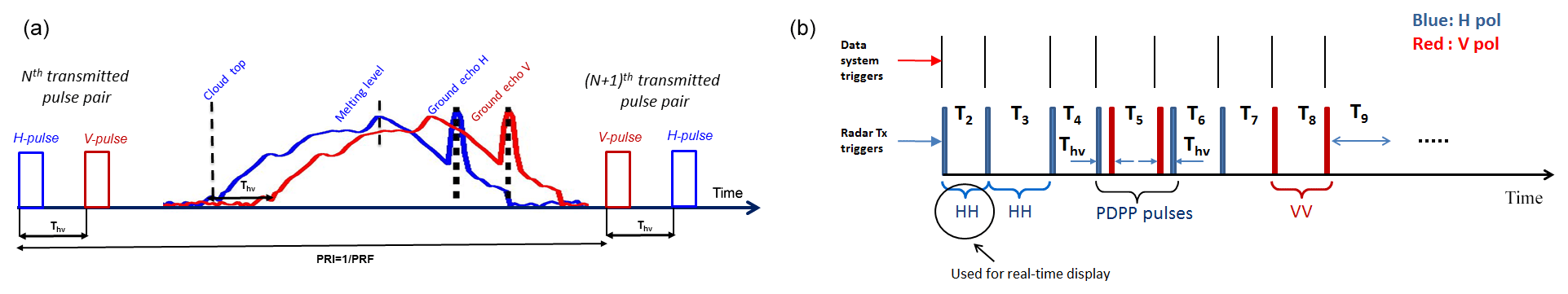
Figure 1(a) Schematic for the polarization diversity pulse mode. The terms H- and V- refer to the polarization state of the outgoing pulses. Pairs of H and V pulses are transmitted with a pulse-pair interval Thv and with a pair repetition interval PRI. Each V–H pair is followed by an H–V pair. Between transmitted pulses, the H (blue) and V (red) receivers sample the backscattered power. (b) A group of 10 pulses (PP10 mode) that contain regular staggered pulse pairs and a PDPP waveform was implemented in the NRC airborne W-band radar system.

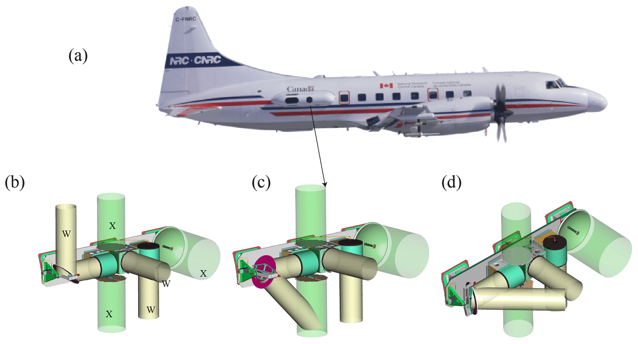
Figure 2(a) The NRC airborne W- and X-band (NAWX) radar installation inside the starboard blister radome mounted on the Convair 580. The aft antenna beam can be redirected from nadir and up to 50∘ forward along the flight direction. The aft antenna beam redirected (b) to the zenith direction using a reflector, (c) to the nadir-forward and (d) to the side-forward directions.
2.1 The NRC airborne W-band radar system
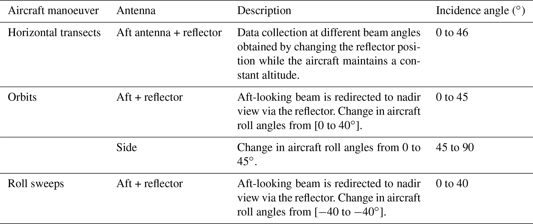
The NRC airborne W- and X-band Polarimetric Doppler Radar system (NAWX) was developed by the NRC Flight Research Lab in collaboration with ProSensing Inc. for the NRC Convair-580 aircraft between 2005 and 2007. The NAWX radar system consists of two single-band subsystems, one operating at W-band (NAW) and another at X-band (NAX). A summary of the NAW system specifications is given in Table 1. The NAWX radar's electronics and data system are rack mounted inside the aircraft cabin while the antenna sub system is housed inside an un-pressurized blister radome (Fig. 2). The NAW antenna subsystem includes three W-band antennas in nadir, aft- and side-looking directions. Two of the antennas, the aft and side antennas, have dual-polarization capability. In addition, a two-axis motorized reflector plate was designed to allow the beam from the aft antenna to be redirected from nadir and up to 50∘ in the forward direction in either horizontal or vertical planes providing Doppler measurement at a wide range of incidence angles. The PDPP data were collected using either the dual-polarization aft-looking antenna and reflector combinations or the side dual-polarization antenna. Radar beam incidence angles ranging from 0 to 80∘ are achieved by performing different aircraft manoeuvres (Table 2). Other unique features of the NAW are listed below.
-
A high quality 1.7 kW peak power air-cooled Extended Interaction Klystron amplifier (EIKA) with a maximum 3 % duty cycle (same as the one used in the CloudSat mission).
-
A two channel 12-bit digital receivers with capability of recording radar raw I and Q data for post processing.
-
An innovative design incorporating NRC-developed INS-GPS integrated navigation system for accurate Doppler correction.
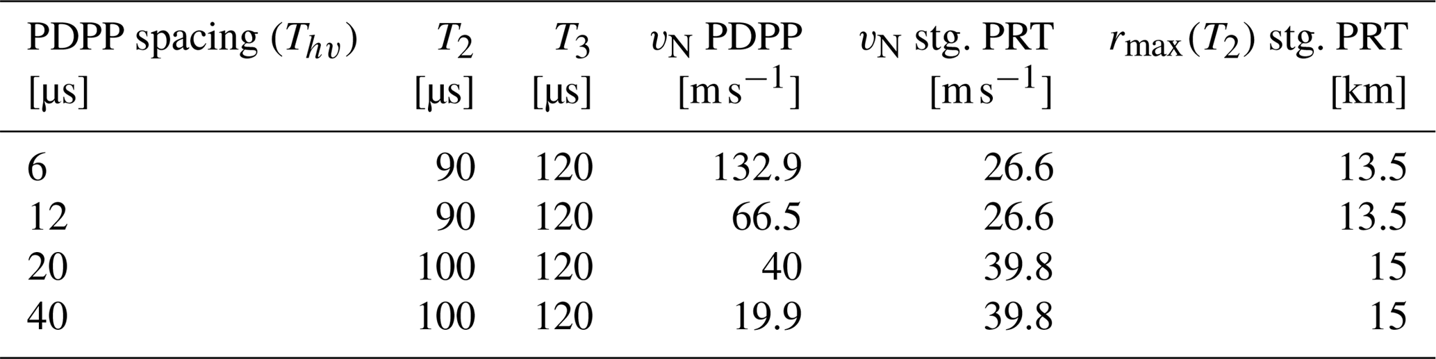
With its unique capability, the NAW is an ideal platform to demonstrate the PDPP technique for airborne and space-borne applications. The NAW radar was originally built using a modulator which was not able to double pulse at very short (of the order of µs) pulse spacings that is required by the PDPP technique. Therefore, the radar was upgraded with a state-of-the-art modulator allowing the radar to double pulse with pulse spacing as small as 0.5 µs. In this mission, PDPP pulse spacing (Thv) of 6, 12, 20 and 40 µs were selected. These specific spacings match integer multiples of the available effective range gate of the radar which is 17.1 m. This eliminates the need to Nyquist sample the return signal and then interpolate the data to co-locate the V and H-pol return gates. In order to efficiently evaluate the performance of PDPP technique, a sequence of and polarization diversity pulse-pairs is interleaved with a conventional staggered pulse repetition time (PRT) waveform (Fig. 1b.). The first three pulses of the waveform form a staggered PRT scheme which extends the unambiguous Doppler velocity range. If the pulse-pair processing is applied to a staggered PRT observation, the maximum unambiguous Doppler velocity is determined by the PRT difference (Zrnic and Mahapatra, 1985). Generally, the staggered PRTs are selected as multiples of a curtained unit time. Zrnic and Mahapatra (1985) have shown that for the pulse-pair technique, the optimal staggered PRT ratio is 2:3. Therefore, the PDPP waveform was designed such that T2:T3 is close to 2:3. Additionally, the pulse spacing T2 and T3 were set according to the maximum desired measurement range – velocity and the transmitter duty cycle limit of the radar. Combinations of T2 and T3 used for this project are given in Table 3.
Pulse spaces should also be small enough to maintain high pulse-to-pulse signal correlation. The normalized signal correlation can be approximated using Eq. (6.5) from Doviak and Zrnić (1993) as
where Td is pulse spacing (PRI), σv is the Doppler velocity spectrum width and λ is the radar wavelength. At the Convair true air speed (va) of 100 m s−1 and antenna beam width θ3 dB of 0.74∘, the aircraft motion induced σv is approximately 0.55 (), assuming a Gaussian antenna beam pattern. In addition, turbulence in the sample volume can further increase σv, so the maximum Td to maintain ρ>0.9 should be less than about 200 µs. However, the PDPP pulse pairs have to be spaced farther than this, so as not to exceed the maximum average transmitter duty cycle. The selected PRTs for PDPP modes are given in Table 3.
2.2 Reflectivity calibration
This section focuses on the calibration of the NAW reflectivity and differential reflectivity measurements. The transmit power, and the gain and noise figure of the two receiver channels were measured by ProSensing Inc. of Amherst, MA, USA using laboratory test equipment, after the PDPP upgrade. Subsequent drifts in the transmitter power were monitored using a coupled detector circuit. Additionally, the receiver gain and noise figure were continuously measured using the Y-factor technique with an internal ambient temperature and heated waveguide terminations in each receiver. The calibration of the remaining sections, such as at the antennas and front-end waveguides, without disassembling the radar, require external reference targets. Water surface and pole-mounted corner reflectors have been tried for calibrations. Using a pole-mounted reflector calibration was problematic due to the difficulty of accurately and consistently pointing a narrow antenna beam at the reflector, while maintaining a high ( dB) reflector signal-to-clutter ratio, without saturating the receiver, so this technique was not employed during the PDPP implementation.
In this work, the end-to-end calibration was done using backscattering properties of the water surface. A detailed description of this method can be found in e.g. Li et al. (2005), Tanelli et al. (2008). In summary, for 94 GHz radars at a 10∘ incidence angle, the mean value of measured σ0 (in clear air conditions) is 5.85 dB with a standard deviation of 0.6 dB (Li et al., 2005). Figure 3 shows the water surface radar cross section (σ0) as a function of incidence angle at different polarizations and with respect to different surface wind directions. It is shown that the horizontal and vertical polarization reflectivity agree very well and there is a crossover point around an incidence angle of 10∘, with near-constant radar cross section regardless of wind direction.

Figure 3Radar cross section of the surface (σ0) as a function of incidence angle: (a) measured σ0 from H polarization over water surface with different wind direction from the 29 March 2016 calibration flight. Gas attenuation and water vapour corrections have not been applied, since the flight in question was performed at a sufficiently low altitude in clear air condition. As a result, the effects of water vapour and gas attenuation are minimal. There is a cross point at incidence angle of around 10∘ and σ0 of 5.85 dB. (b) σ0 from both horizontal and vertical polarizations for 4 March 2017 flight shows a good polarimetric calibration.
The airborne PDPP flights were conducted from March 2016 to April 2017. We collected a total of over 31 flight hours of PDPP data (4 TB) from 22 flights over diverse weather (clear air, cloud and precipitation systems) and surface conditions (open water, snow and land). Most of the open water flights were conducted over the Great Lakes region. However, dedicated PDPP flights were also flown over the Pacific and Atlantic Oceans. These flights were conducted in diverse wind conditions, which allowed for characterization of the radar cross section at varying wind conditions. Values of σ0 in various surface conditions and sea states at elevation angles ranging from near nadir to 80∘ were analyzed (Battaglia et al., 2017). In this paper, we focus our observations and analysis of the PDPP data during two weather flights.
As presented in Sect. 2, the PDPP data collection was obtained using two fixed antennas and a reflector that allowed redirecting one of the fixed antennas (aft-looking) into the desired beam angles. Figure 4 shows a typical flight track during the PDPP data collections, where the aircraft sampled a region of interest by performing a series of horizontal transects, roll sweeps and orbit manoeuvres. This allowed accumulating data at various PDPP configurations as well as beam angles ranging from near 0 to about 80∘. Table 2 summarizes aircraft manoeuvres used in the PDPP data collections.
The location and range of the ground return and Doppler velocity from the platform-motion depend on the antenna used and the aircraft manoeuvre. Figures 5–6 show examples of the aircraft and ground-beam tracks obtained using the side and aft antennas during a roll sweep manoeuvre. For the side antenna, the platform motion plus the measured Doppler velocity is generally less than 20 m s−1 even at the maximum steep roll angle (≈50∘) at the Convair's mean true air speed of 100 m s−1. In contrast, when using the aft antenna and redirecting the beam forward along the flight direction, the platform motion contribution to the Doppler velocity can exceed 100 m s−1.

Figure 4Typical PDPP flight track showing where the aircraft performed a series of horizontal transects (HT), roll sweeps (RS) and orbits of various roll angles.

Figure 5(a) The NRC Convair-580 flight track (red) and the beam ground track (orange) during a PDPP data collection flight on 10 January 2017. The beam ground track show the side antenna beam ground track while the aircraft is performing a partial roll sweep manoeuvre. The inserts at the bottom of the image show aircraft (b) pitch angle, (c) roll angle, (d) beam incidence angle and aircraft altitude.
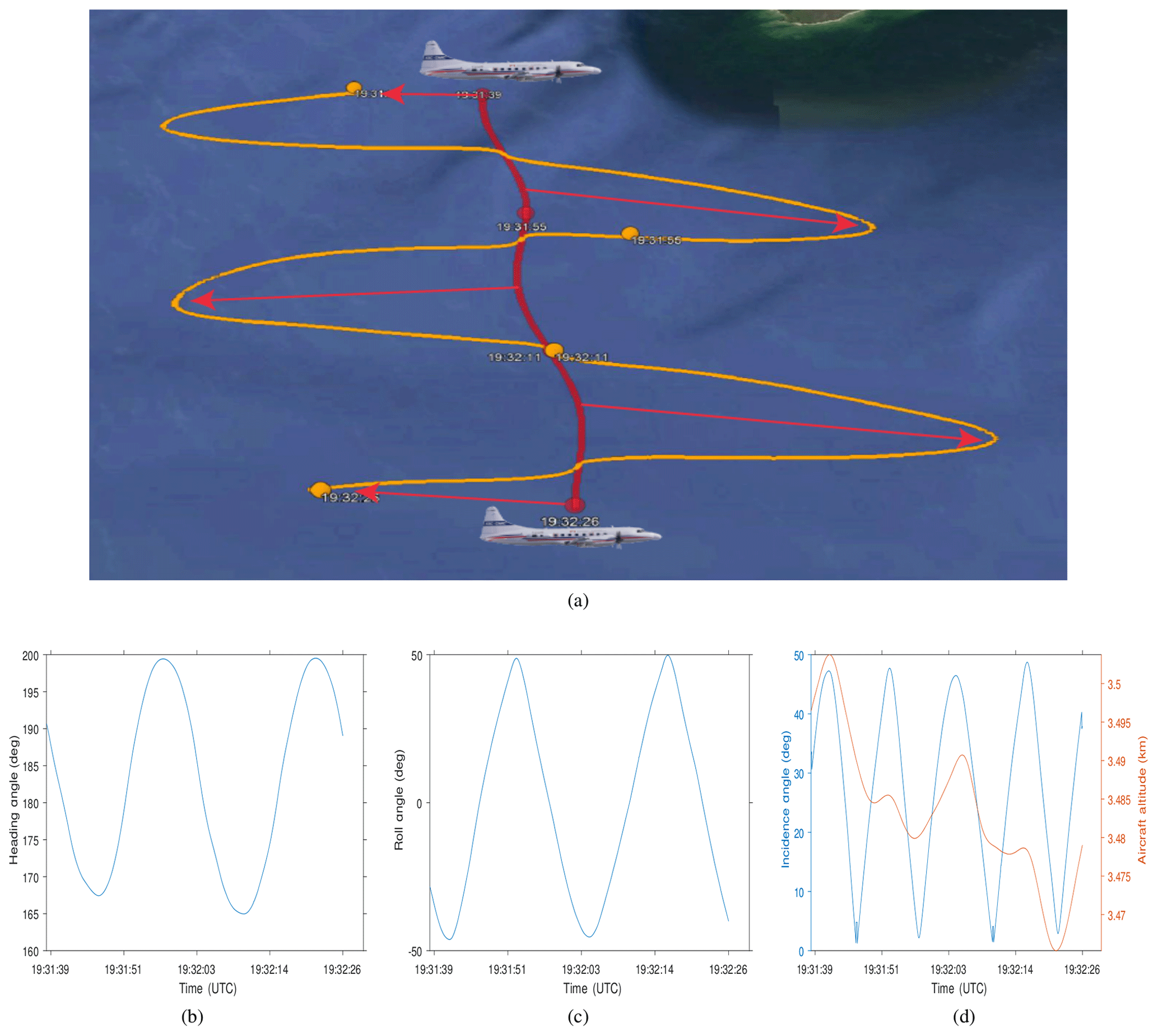
Figure 6Example of beam angle from aft antenna redirected to nadir by the reflector and the aircraft performing a roll sweep from ∘ over Lake Ontario on 27 January 2017.
The goals of the field campaign were as follows:
-
to characterize the σ0 and the cross-pol signatures of ocean and land surfaces;
-
to use the characterization of σ0 in order to portray a typical ground surface clutter and the resultant surface blind zone;
-
to investigate the presence of ghosts associated with cross polar returns induced both by the surface and by meteorological targets;
-
to check the validity of the dependence of the variance of the velocity estimates on the signal-to-noise ratio (e.g. on different reflectivities or different cloud systems), the signal-to-ghost ratio, the Thv and the number of samples.
The first two goals were addressed in a previous paper (Battaglia et al., 2017); the foci of this paper are on the last two project goals.
4.1 Ghost echoes and impacts on PDPP velocity estimates: theoretical considerations
The key assumption underpinning the polarization diversity methodology is that the H- and V- pulses are independent. Cross-coupling between the two polarizations can occur either at the hardware level or can be induced during radar beam interactions with the hydrometeors (propagation and/or backscattering in the atmosphere). While the former is typically reduced to values lower than −25 dB, the latter can be important and is characterized by the linear depolarization ratio (LDR). LDR values depend on hydrometeor types and radar beam angles. For example, melting crystals produce high LDR signatures at low to high radar beam incidence angles while for columnar crystals, LDR values increase with radar beam angle. For 94 GHz radars at large incidence angles (e.g. 40∘ for WIVERN), atmospheric hydrometeors like melting snowflakes and columnar crystals produce LDR up to −12 dB (Wolde and Vali, 2001a, b). From measurements done by the NRC airborne W-band radar, surfaces tend to strongly depolarize with characteristic values of −10 and −15 dB over land and over sea, respectively (Battaglia et al., 2017). The effect of cross-polarization is the production of an interference signal in both H and V receiver channels. The strength of such interference at sampling time t depends on the strength of the cross-polar signal at the time t shifted by the time separation Thv (forward or backward depending upon whether the receiving channel corresponds to the polarization of the first or of the second pulse of the pair). When converted into range, r, the voltages measured in the two orthogonal receiving channels can be expressed as follows:
where and 𝒱ij is the voltage at the output of the i-polarized receiver when j polarization is transmitted, and 𝒩V and 𝒩H represent the system noise in the vertical and horizontal receiver channels, respectively. Here we have assumed that the H-pulse is the first pulse emitted (like for the first pair of Fig. 1). The powers can be computed from averaging the modular square of the voltages, e.g. , , and .
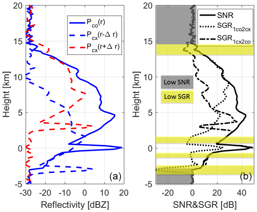
Figure 7Example of cross talk interference in the PDPP scheme for a reflectivity profile extracted from CloudSat (a −28 dBZ equivalent noise power for the H- and V-channel is assumed). (a) The V-pulse produces both a co-polar (PVV) and a cx-polar return (PHV); the same is true for the H-pulse. An LDR of −15 dB and a Thv=20 µs (corresponding to a height separation of 3 km at nadir incidence) are assumed. (b) Signal-to-noise ratio (black) and signal-to-ghost ratios as defined in Eqs. (4)–(5). The gray areas identify regions with SNR<3 dB and the yellow bands regions with SGRs<0 dB.
In the left panel of Fig. 7 the co-polar power (continuous line) and cross-polar powers (dashed lines) are depicted for a plausible profile (the co-polar profile is extracted from a CloudSat observation) with the cross-polar signals derived under the assumption of a constant dB for the whole profile. There are two possible sources of cross-coupling:
-
The co-polar signal of the first pulse of the pair, P1co, (continuous blue) interferes with the cross coupling of the second pulse, P2cx, at a range reduced by (dashed blue line, second term on the right-hand side of Eq. 2);
-
The co-polar signal of the second pulse of the pair, P2co, (continuous blue) interferes with the cross coupling of the first pulse, P1cx, at a range increased by (dashed red line, second term on the right-hand side of Eq. 3).
In the power domain, these interferences contribute to the measured co-polar backscattering signal and sometimes can exceed it (e.g. in the left panel of Fig. 7 near the cloud top at 14.5 km height), thus appearing as “ghost echoes” (Battaglia et al., 2013). To quantify the strength of the interference signals it is useful to define the “signal-to-ghost ratios” (SGR) as follows:
These quantities are depicted in the right panel of Fig. 7 for the profile shown on the left panel.
Because crosstalk signals come from different range gates, they are independent of the co-polar echoes and do not bias the velocity estimates. However, ghost echoes increase the velocity estimation error as a function of the signal-to-ghost ratio (SGR). There are two possible ways to predict the increase in the variance of the mean velocity estimate. In the first approach, following Pazmany et al. (1999), the variance of the mean velocity estimate for the V–H pair, , can be estimated as follows:
where Rvh(r,Thv) is the cross-correlation function at lag Thv which can be estimated as follows:
while the variance on the right-hand side can be computed as (see Appendix in Pazmany et al., 1999):
where M (V–H) pairs have been considered. Here SNRH and SNRV stand for signal-to-noise ratios of the H and V signals, respectively ( and ).
The expression in Eq. (8) shows that SGR values lower than 1 (0 dB) can become increasingly detrimental for the variance, which is inversely proportional to the number of sampled pairs. A similar expression is valid for the (H–V) pair.
In a second approach, the variance of the velocity estimates is completely characterized by the observed correlation between pairs of H and V pulses, ρobs(Thv), defined as follows:
which accounts for the effects of the target repositioning (decorrelation), of noise and of the crosstalk introduced by the ghosts. For instance, an increase of noise increases the denominator and produces a drop in ρobs. If we can assume independent sample pairs (which is typically true if the PRI is longer than the decorrelation time) then the variance of the pulse-pair velocity estimates can be expressed as (Doviak and Zrnić, 1993):
where M (V–H) pairs have been considered. Since the velocity estimate is obtained from the average of V–H and H–V pulse-pair phase measurements then the variance of the velocity estimate will be
The approaches described above both confer advantages and limitations. Selecting which one to use then depends on the application in question. The first approach is very useful in simulation frameworks; in such conditions the voltage signals described in Eqs. (2)–(3) can be neatly separated into all three of their components and therefore all the terms in Eqs. (6)–(8) can be derived ( can be estimated from the Doppler spectral width). On the other hand, the second approach Eq. (10) provides an estimate of the variance of the velocities directly from an observable (the observed correlation, ρobs). This allows an inherent assessment of the measurement-derived Doppler signal quality.
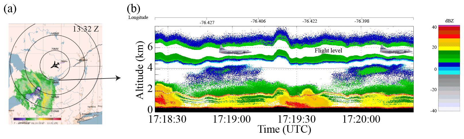
Figure 8(a) Screen capture of NexRad Buffalo S-band radar received at the aircraft as it leaves Ottawa, ON, Canada on 10 January 2017. (b) Vertical cross section of reflectivity obtained by the NRC airborne X-band (NAX) radar while the aircraft is sampling a cloud system over Lake Ontario.
4.2 Field campaign case studies
In this section, we will present two different flight segments where PDPP data were collected while the aircraft sampled winter clouds.
4.2.1 Case 1 (10 January 2017): ghost echoes and impacts on PDPP velocity estimates
In this flight the Convair made extensive samplings of a frontal system over Lake Ontario and its surrounding regions in Ontario, Canada and the state of NY, USA. Figure 8a shows a screen capture of a Buffalo NexRad image received using the onboard datalink as the aircraft departed Ottawa to sample the precipitation system that covered Lake Ontario and part of Lake Huron. The NAW was run in PP10 mode (10 conventional pulse-pairs) for the initial portion of the flight supporting other objectives, and then switched to PDPP mode for the remainder of the flight duration, during which the aircraft sampled the tail of a winter storm over Lake Ontario.
During the PDPP data collection, the aircraft first performed repeated roll sweep manoeuvres by varying the roll angles , and then performed an orbit manoeuvre using the side antenna. Winds at the flight level of ≈5 km were north-west at 30 m s−1. For this case, we selected to highlight the PDPP observations during the orbit manoeuvre using the side dual-pol antenna. As the W-band measurement was limited to nadir or nadir-fore view, the X-band reflectivity profile showing the aircraft altitude with respect to ground and cloud and precipitation structures is shown in Fig. 8b. The aircraft was just below the cloud top, but there was a break in the cloud layer below with a stronger Ze value extending from the surface to about 1.5 km.
A segment of the flight track performed between 17:19 and 17:20:04 UTC over the north-eastern bank of Lake Ontario is shown in Fig. 5. For this data file, Thv is set to 12 µs (equivalent to 900 m). The aircraft performed a complete circle with roll angles between 39 and 49∘, at an altitude of 4 km. As a result, the range to the surface is changing between 5.8 and 6.2 km.
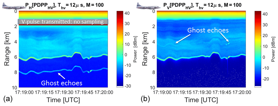
Figure 9Example of power as recorded when operating in PDPP mode with H-pulse followed by a V-pulse after 12 µs. (a) Power received in the H-channel; (b) power received in the V-channel. The mechanism for producing ghost echoes is explained in the upper part of the panel.
The received powers in the H and V-channel when the radar was operating in PDPP mode are shown in Fig. 9. Even if the roll and beam angle changes are modest during the aircraft orbit manoeuvre, there is still significant change to the surface Ze values, likely due to a change in surface water wave patterns, water surface targets such as boats, and other ground targets. The linear depolarization ratio (not shown) clearly shows enhanced areas of LDR (approximately between −15 and −12 dB) in correspondence to the surface. In contrast, LDR from hydrometeors were not detectable except when at close range to the aircraft. Note that the H-receiver must be turned off when the V-pulse is sent out, which corresponds to a blind layer in the left panel. Since the power P is depicted (and not reflectivity), targets at close ranges produce larger signals (since ).
The ghost echoes and returns shown in Fig. 9 appear in both H & V channels at different ranges. As explained in Sect. 4.1 these ghosts are the result of cross talk occurring at the same range increased (left panel) or decreased (right panel) by cThv∕2 which in this case is equal to 1.8 km. Two kind of ghosts are clearly detectable (see white arrows): those related to the surface and those produced just after a range equal to cThv∕2 associated with the enhancement of backscattered power by targets at very short ranges. The latter are spurious effects which will not be produced in a space-borne configuration (when all targets are basically at the same distance).
The signal-to-ghost ratios, as defined by Eqs. (4)–(5), are plotted in two panels of Fig. 10. The areas with blue colours correspond to regions where the magnitude of the ghosts is comparable or larger than the magnitude of the signal and will be therefore characterized by a significant reduction in Doppler accuracy, as previously discussed. On the left panel the extended area of small SGR just after a range of 1.8 km is caused by the interference of the cross-polar signal at very short ranges; other ghosts are present below the surface range. On the other hand, the key features observable on the right panel of Fig. 10 are found in correspondence to ranges 1.8 km shorter than the surface range. This is caused by the strong cross-pol signal of the first pulse in the pair.
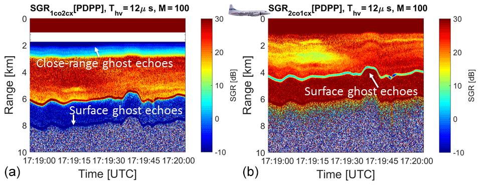
Figure 10Signal-to-ghost ratios as defined by Eqs. (4)–(5). Areas with blue colours will have a significant reduction in Doppler accuracy due to the additional noise produced by the ghosts. Note on the right panel the extended area of small SGR caused by the interference of cross-polar signal at very short ranges.
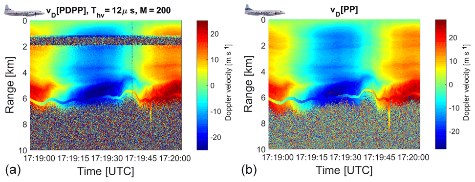
Figure 11Velocity as measured by the PDPP technique with Thv=12 µs (a) and by the pulse-pair with two staggered pulse repetition times of 90 and 120 µs (b).
Figure 11 shows a comparison of the Doppler velocities as measured via a PDPP sequence with Thv=12 µs ( m s−1) and a conventional PP technique using two staggered PRFs ( m s−1) (Torres et al., 2004). The line of sight winds are seen to change as expected, with a sinusoidal pattern in time, clearly mirroring the change in the heading of the aircraft (see Fig. 5). The estimates have been done using 100 H–V plus 100 V–H pairs and 100+100 staggered conventional and pairs (corresponding to roughly 20 km integration in the WIVERN configuration). The vD from PDPP is similar to the one estimated using standard PP, except for those ranges when the receiver was turned off because of the transmission in the other channel. In that situation the velocity is a random number within the Nyquist interval (like in all the other regions dominated by noise).
For better comparison we have used the same scale between −26.6 and 26.6 m s−1 for the Doppler velocities (but in the left panel the velocities range between −66.5 and +66.5 m s−1). In this scenario there were no high winds and therefore the staggered pulse-pair Nyquist interval was good enough for measuring the Doppler velocities (though there are a few aliased points close to the surface at about 17:19:22 UTC), but of course the PDPP has the potential to unambiguously measure much higher velocities. However, this improvement is not without drawback, as PDPP produces a noisier estimate of the Doppler velocities (compare the two panels), particularly in presence of low SGRs (e.g. SGR<0 like in correspondence with the blue-coloured regions highlighted by the white arrows in the two panels of Fig. 10).
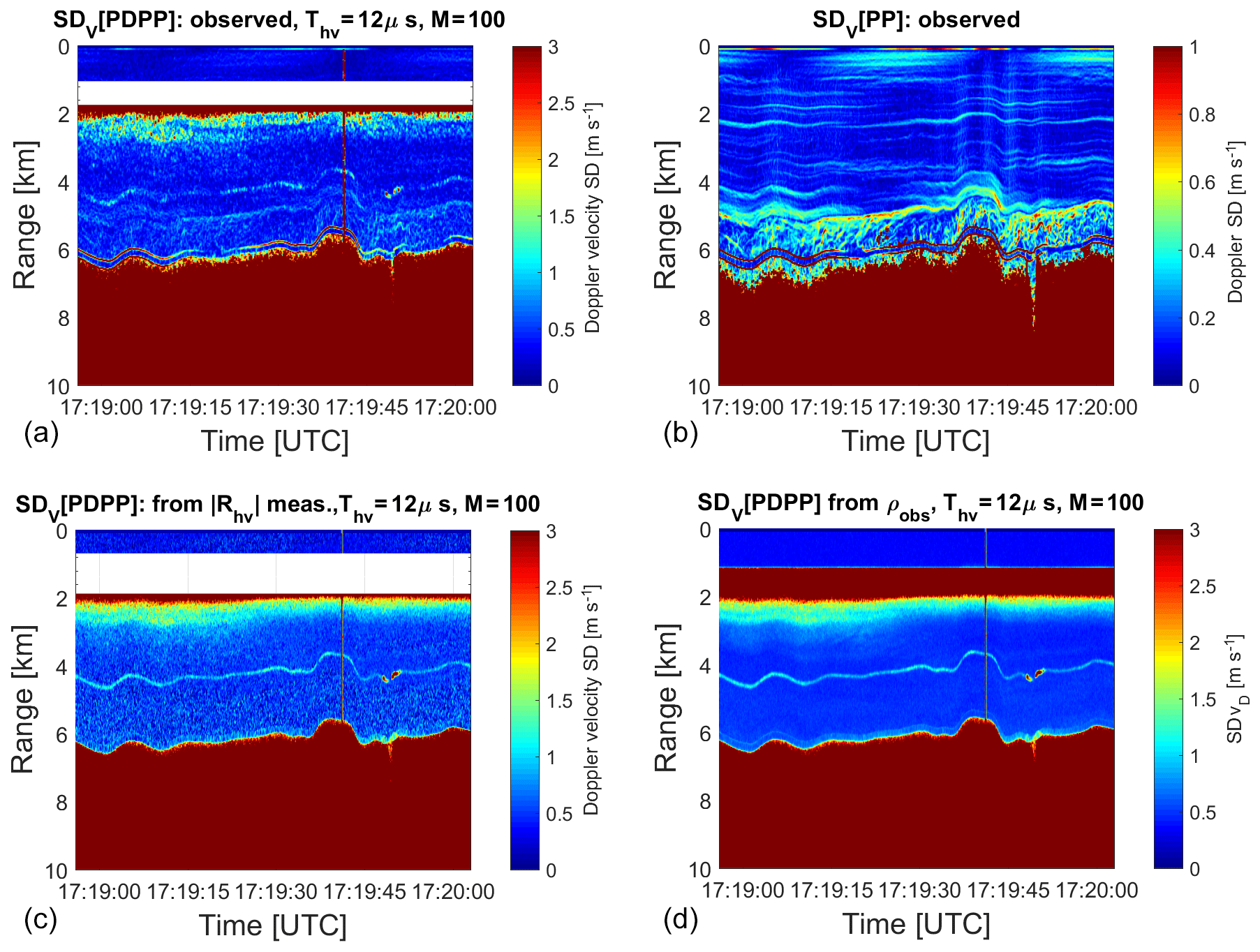
Figure 12(a, b) Standard deviation of Doppler velocity estimated from the spatial variability of the velocity fields shown in Fig. 11 for the PDPP (a, c) and PP (b, d) technique, respectively (note different scales for the colourbar). Standard deviation of Doppler velocity as derived from Eq. (8) (c) and Eq. (10) (d).
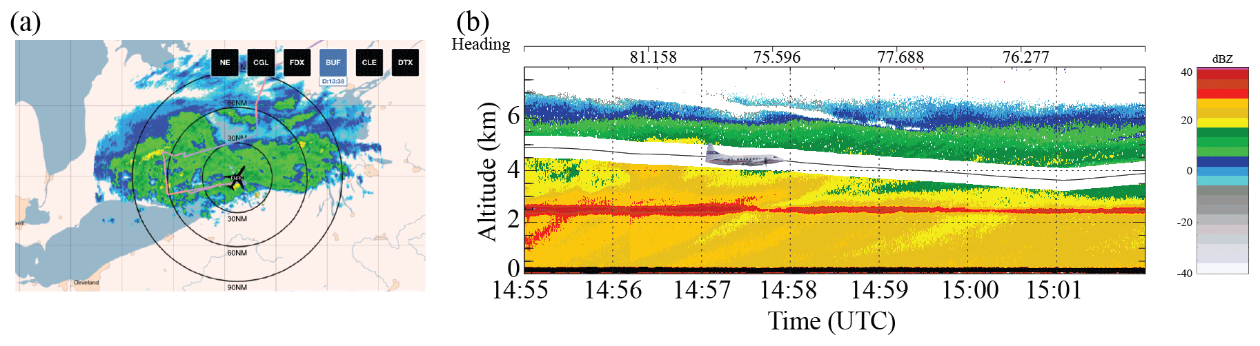
Figure 13Same as Fig. 8 except during the PDPP data collection inside a winter storm on 25 March 2017.
As a proxy for the velocity estimate standard deviation, the standard deviation was computed for each point, using a 3×3 pixel window centred on each position (in time and space); results are shown in Fig. 12 for the PDPP (top left) and the PP (top right) estimates. This will be referred to as the velocity standard deviation estimated from the spatial and temporal variability. This method might overestimate the velocity standard deviation, because it has enhanced values in correspondence to strong spatial gradients of the Doppler velocities (e.g. in the region about 1 km above the surface). The PP is clearly significantly better (note that the colourbar scale is ranging from 0 to 1 m s−1), with the PDPP performing particularly poorly in correspondence to the surface and to the close range ghost echoes. On the other hand, the velocity standard deviation can be computed using either Eq. (8) (see bottom left panel) or Eq. (10) (see bottom right panel). In the first case all the quantities that appear on the right-hand side of Eq. (8), except for |Rvh(r,Thv)| which is estimated via Eq. (7), must be computed from the measurements in PP mode. This requires firstly an estimation on a ray by ray basis, for the noise levels in the two receiver channels, and secondly an estimate of the noise-subtracted co- and cross-polar powers. Finally, from these estimations, SNRs and the SGRs are both computed. Both techniques produce results very similar to the velocity standard deviation estimated from the spatial variability with the largest discrepancies concentrated in areas where the Doppler velocity field is rapidly changing (compare with the left panel in Fig. 11), though the results in the left bottom panel are noisier. Again, it is useful to underline that Eq. (10) can be directly applied to an observed variable (the observed correlation). Not only does the PDPP allow for the estimation of the Doppler velocity but also its expected accuracy.
4.2.2 Case 2 (25 March 2017): extreme Doppler velocity measurements
For this case, we highlight instances of high VD from the PDPP measurement inside a major winter storm on 25 March 2017. The Convair flew for over 5 h sampling the winter storm over land near Buffalo, NY, over Lake Huron and Lake Ontario as the frontal system moved towards south-eastern Ontario. Figure 13 shows a screen capture of the US Buffalo NexRad Ze and the Ze profiles of the NRC airborne X-band (NAX) radar corresponding to the PDPP data segment of Case 2. The NAX Ze imagery shows the aircraft descended from about an altitude of 4.8 to 4 km and remained in cloud above a well defined melting layer (2.5 km). The PDPP data were collected using the aft antenna and reflector combinations while the aircraft is performing a horizontal transect and descending from 5 to 4.4 km.
The use of the aft antenna in combination with the reflector provides a unique means to direct the antenna beam to a wide range of positions. By steering the aft antenna's beam to a large slant angle, the maximum Doppler velocity introduced by the aircraft motion can reach up to 100 m s−1, which makes a good test for evaluating the PDPP method's high velocity retrieval capability. Figure 14 shows the aircraft flight track, the beam ground intersection track, the aircraft altitude, as well the beam incidence angle during the 25 March 2017 flight. The beam position began at nadir, and was steered to the reflector limit (50∘ incidence angle) at which point the beam was then moved back to the nadir position in step decrements of 10∘. The PDPP spacing (Thv) for this case was set at 6 µs (900 m) which provides a maximum unambiguous Doppler of 132.9 m s−1 (Table 3).

Figure 14Flight track and beam configuration during the PDPP data collection on 25 March 2017. (a) The NRC Convair-580 flight track (red) and the radar beam ground-track (orange). The locations of the two radiosonde stations, Buffalo, NY (BUF) and Maniwaki, Quebec (WMV) and Ottawa (YOW) are also shown to aid the interpretation of the data presented in Fig. 13. (b) Aft-antenna beam incidence angle and aircraft altitude.
Figure 15 shows PDPP reflectivity fields measured during this stepped change in the reflector's angle. There was a well-defined melting layer at around 2.5 km (consistent with the NAX Ze profile shown in Fig. 13b), which can be seen at the beginning of this segment when the antenna beam was at nadir position. As the antenna beam moved forward toward the flight path, the ground and melting layers appear at different radar range. Similar to the case study in Sect. 4.2.1, ghost echoes associated with the ground and melting layer are observed in the second PDPP pulse reflectivity (Zhh and Zvh in Fig. 15).

Figure 15Similar to Fig. 9 but for 25 March flight and in reflectivity space. The PDPP spacing in this case is 6 µs.
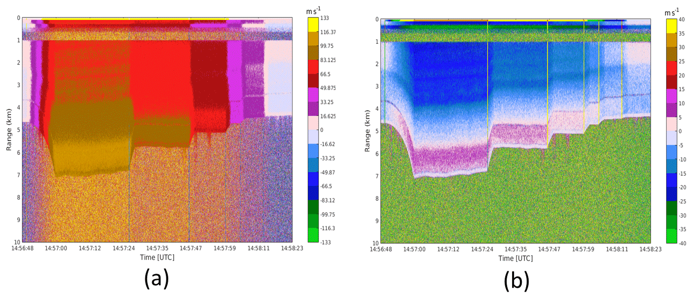
Figure 16Velocity fields for the case study in Fig. 15: (a) measured PDPP velocity and (b) estimated velocity of the precipitation along the direction of the antenna beam based on PDPP measurements and after removal of aircraft motion.
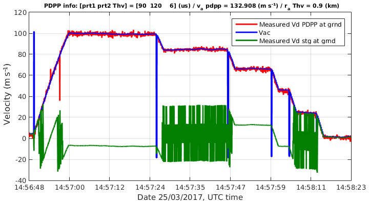
Figure 17PDPP measured velocity (red line), the aircraft contribution computed from the aircraft INS data (blue line) and velocity estimates using staggered PRT pulses (green) at ground gates for the study case in Fig. 13.
The measured PDPP Doppler velocity was properly retrieved using a method described in Nguyen and Wolde (2019) is depicted in Fig. 16a. The measured Doppler was as high as 100 m s−1 in regions where the reflector was steered at and reduced to a few m s−1 when the reflector moved back to nadir position. In all scenarios, PDPP technique works very well. There was almost no velocity folding even at weak signal regions (around 14:57:12 UTC and at 6 km altitude). A comparison of Vd obtained from PDPP with the conventional staggered PRT techniques is shown in Fig. 16. Due to a much narrower Nyquist range, staggered PRT velocity was folded many times. This case is a successful example of using the PDPP technique to measure very high radial Doppler velocity in order to obtain accurate horizontal winds from space.
Figure 16b depicts the Doppler velocity after removing the aircraft motion. Once the aircraft contribution into the Doppler velocity is removed, the vD estimates are a combination of the hydrometeor's terminal velocity as well as the wind along the line of sight. In this case, the hydrometeor's terminal velocity can be neglected except in rain, below the melting layer and when the beam is in nadir position. It can be seen that the strongest Doppler velocity after removing the platform motion was recorded when the Aft antenna beam was redirected nearly 50∘ forward along the flight direction (14:57:00–14:57:24). In this high vD segment, the vD was negative (away from the radar) between flight levels with slightly decreasing magnitude from −20 m s−1 at the flight level to nearly 0 m s−1 at around 5.5 km range. The vD became positive (towards the radar) between the surface 5.5 km radar range. The PDPP vD profiles are consistent with the vertical profile of horizontal wind measured by the aircraft and radiosonde soundings of nearby stations (not shown).
This work describes the implementation of polarization diversity on the NRC airborne W-band radar and the novel results collected during different flights conducted over North America in 2016 and 2017. This was the first time a PDPP mode has been implemented on a W-band radar on a moving platform. The conclusions of this study can be summarized as follows:
-
A comprehensive PDPP I&Q dataset has been collected, which allows characterizing PDPP-based Doppler velocity estimates in various environmental conditions.
-
The polarization diversity technique allowed much larger velocity to be measured unambiguously. Doppler velocities exceeding 100 m s−1 were measured during the field campaign when adopting a pulse-pair separation Thv equal 6 µs.
-
Crosstalk between the two polarizations caused by depolarization at backscattering deteriorated the quality of the observations by introducing “ghost echoes” in the power signals and by increasing the noise level in the Doppler measurements. The regions affected by crosstalk were generally associated with the strongly depolarizing surface returns and to the depolarization of hydrometeors located at short ranges from the aircraft.
-
The increased variance in Doppler velocity estimates were well predicted in cases where the signal-to-noise and signal-to-ghost ratios are known (Eqs. 6–8) or in cases where the observed correlation between the H-polarized and V-polarized successive pulses was measured (Eq. 10). The first approach can be used in simulation frameworks and end-to-end simulators; the second can be used to estimate the quality of the Doppler measurements directly from the observations themselves.
-
The airborne field campaign has also provided novel observations of the backscattering properties of sea and land surfaces at W-band at viewing angles larger than 30∘. This is the topic of a companion paper (Battaglia et al., 2017).
The measurement of 3-D atmospheric winds in the troposphere remains one of the great priorities of the next decade (The Decadal Survey, 2017) and polarization diversity offers a solution to the short decorrelation expected from fast moving platforms. Different concepts are currently being examined by different agencies (Durden et al., 2016; Illingworth et al., 2018a). This study provided a full proof-of-concept for an airborne W-band Doppler radar equipped with polarization diversity and therefore represents a key milestone towards the implementation of polarization diversity in space.
The project data has been submitted to the ESA. A request for the data can be submitted to the ESA by referring the ESA-ESTEC contract no. 4000114108/15/NL/MP.
AI is the PI for the project, and MW and AB are members of the science team that developed the ESA proposal. ALP came up with a design to modify the NRC W-band radar to have PDPP capability. MW was the flight mission scientist for all the flights and CN flew during most of the research flights and operated the radar. CN wrote the code for processing the I&Q data. MW, CN and their student Kenny Bala generated all the figures except Figs. 1a and 7 that were generated by AB. The paper is written by MW, AB and CN. AI and ALP have provided contents for sections of the paper and also reviewed the draft and made some changes to the original draft.
The authors declare that they have no conflict of interest.
This work was supported in part by the European Space Agency under the
activity Doppler Wind Radar Demonstrator (ESA-ESTEC) contract no.
4000114108/15/NL/MP and in part by CEOI-UKSA under contract RP10G0327E13. We
acknowledge the support from the NRC flight and support staff during the
flight campaign. We would like also to thank the Carleton University co-op
student Kenny Bala, who generated some of the figures used in the paper.
Edited by: Murray Hamilton
Reviewed by: three anonymous referees
Battaglia, A. and Kollias, P.: Error Analysis of a Conceptual Cloud Doppler Stereoradar with Polarization Diversity for Better Understanding Space Applications, J. Atmos. Ocean Technol., 32, 1298–1319, https://doi.org/10.1175/JTECH-D-14-00015.1, 2014. a
Battaglia, A., Tanelli, S., Kobayashi, S., Zrnic, D., Hogan, R., and Simmer, C.: Multiple-scattering in radar systems: a review, J. Quant. Spectrosc. Ra., 111, 917–947, https://doi.org/10.1016/j.jqsrt.2009.11.024, 2010. a
Battaglia, A., Augustynek, T., Tanelli, S., and Kollias, P.: Multiple scattering identification in spaceborne W-band radar measurements of deep convective cores, J. Geophys. Res., 116, D19201, https://doi.org/10.1029/2011JD016142, 2011. a
Battaglia, A., Tanelli, S., and Kollias, P.: Polarization diversity for millimeter space-borne Doppler radars: an answer for observing deep convection?, J. Atmos. Ocean Technol., 30, 2768–2787, https://doi.org/10.1175/JTECH-D-13-00085.1, 2013. a, b
Battaglia, A., Wolde, M., D'Adderio, L. P., Nguyen, C., Fois, F., Illingworth, A., and Midthassel, R.: Characterization of Surface Radar Cross Sections at W-Band at Moderate Incidence Angles, IEEE T. Geosci. Remote, 55, 3846–3859, https://doi.org/10.1109/TGRS.2017.2682423, 2017. a, b, c, d
Battaglia, A., Dhillon, R., and Illingworth, A.: Doppler W-band polarization diversity space-borne radar simulator for wind studies, Atmos. Meas. Tech., 11, 5965–5979, https://doi.org/10.5194/amt-11-5965-2018, 2018. a
Bessho, K., Date, K., Hayashi, M., Ikeda, A., Imai, T., Inoue, H., Kumagai, Y., Miyakawa, T., Murata, H., Ohno, T., Okuyama, A., Oyama, R., Sasaki, Y., Shimazu, Y., Shimoji, K., Sumida, Y., Suzuki, M., Taniguchi, H., Tsuchiyama, H., Uesawa, D., Yokota, H., and Yoshida, R.: An introduction to Himawari-8/9 – Japan's new-generation geostationary meteorological satellites, J. Meteor. Soc. Jpn., 94, 151–183, https://doi.org/10.2151/jmsj.2016-009, 2016. a
Bluestein, H. B. and Pazmany, A. L.: Observations of Tornadoes and Other Convective Phenomena with a Mobile, 3-mm Wavelength, Doppler Radar: The Spring 1999 Field Experiment, B. Am. Meteorol. Soc., 81, 2939–2951, 2000. a
Bluestein, H. B., Weiss, C. C., and Pazmany, A.: The Vertical Structure of a Tornado near Happy, Texas, on 5 May 2002: High-Resolution, Mobile, W-band, Doppler Radar Observations, Mon. Weather Rev., 132, 2325–2337, 2004. a
Doviak, R. J. and Zrnić, D. S.: Doppler Radar and Weather Observations, Academic Press, 1993. a, b
Durden, S. L., Siqueira, P. R., and Tanelli, S.: On the use of multi-antenna radars for spaceborne Doppler precipitation measurements, IEEE Geosci. Remote Sens. Lett., 4, 181–183, 2007. a
Durden, S. L., Tanelli, S., Epp, L. W., Jamnejad, V., Long, E. M., Perez, R. M., and Prata, A.: System Design and Subsystem Technology for a Future Spaceborne Cloud Radar, IEEE Geosci. Remote Sens. Lett., 13, 560–564, 2016. a, b
Illingworth, A. J., Barker, H. W., Beljaars, A., Chepfer, H., Delanoe, J., Domenech, C., Donovan, D. P., Fukuda, S., Hirakata, M., Hogan, R. J., Huenerbein, A., Kollias, P., Kubota, T., Nakajima, T., Nakajima, T. Y., Nishizawa, T., Ohno, Y., Okamoto, H., Oki, R., Sato, K., Satoh, M., Wandinger, U., and Wehr., T.: The EarthCARE Satellite: the next step forward in global measurements of clouds, aerosols, precipitation and radiation, B. Am. Meteorol. Soc., 96, 1311–1332, https://doi.org/10.1175/BAMS-D-12-00227.1, 2015. a
Illingworth, A. J., Battaglia, A., Bradford, J., Forsythe, M., Joe, P., Kollias, P., Lean, K., Lori, M., Mahfouf, J.-F., Mello, S., Midthassel, R., Munro, Y., Nicol, J., Potthast, R., Rennie, M., Stein, T., Tanelli, S., Tridon, F., Walden, C., and Wolde, M.: WIVERN: A new satellite concept to provide global in-cloud winds, precipitation and cloud properties, B. Am. Meteorol. Soc., 99, 1699–1687, https://doi.org/10.1175/BAMS-D-16-0047.1, 2018a. a, b, c, d, e
Illingworth, A. J., Battaglia, A., Delanoe, J., Forsythe, M., Joe, P., Kollias, P., Mahfouf, J.-F., Potthast, R., Rennie, M., Tanelli, S., Viltard, N., Walden, C., Witschas, B., and Wolde, M.: WIVERN (WInd VElocity Radar Nephoscope), Proposal submitted to ESA in response to the Call for Earth Explorer-10 Mission Ideas, 2018b. a
Kobayashi, S., Kumagai, H., and Kuroiwa, H.: A Proposal of Pulse-Pair Doppler Operation on a Spaceborne Cloud-Profiling Radar in the W Band, J. Atmos. Ocean Technol., 19, 1294–1306, https://doi.org/10.1175/1520-0426(2002)019<1294:APOPPD>2.0.CO;2, 2002. a
Kollias, P., Tanelli, S., Battaglia, A., and Tatarevic, A.: Evaluation of EarthCARE Cloud Profiling Radar Doppler Velocity Measurements in Particle Sedimentation Regimes, J. Atmos. Ocean Technol., 31, 366–386, https://doi.org/10.1175/JTECH-D-11-00202.1, 2014. a
Lhermitte, R.: Attenuation and Scattering of Millimeter Wavelength Radiation by Clouds and Precipitation, J. Atmos. Ocean Technol., 7, 464–479, 1990. a
Li, L., Heymsfield, G. M., Tian, L., and Racette, P. E.: Measurements of Ocean Surface Backscattering Using an Airborne 94 GHz Cloud Radar- Implication for Calibration of Airborne and Spaceborne W-Band Radars, J. Atmos. Ocean Technol., 22, 1033–1045, https://doi.org/10.1175/JTECH1722.1, 2005. a, b
Matrosov, S. Y., Battaglia, A., and Rodriguez, P.: Effects of Multiple Scattering on Attenuation-Based Retrievals of Stratiform Rainfall from CloudSat, J. Atmos. Ocean Technol., 25, 2199–2208, https://doi.org/10.1175/2008JTECHA1095.1, 2008. a
Nguyen, C. and Wolde, M.: NRC W-band and X-band airborne radars: signal processing and data quality control, Geoscientific Instrumentation, Methods and Data Systems Discussions, in preparation, 2019. a
Pazmany, A., Galloway, J., Mead, J., Popstefanija, I., McIntosh, R., and Bluestein, H.: Polarization Diversity Pulse-Pair Technique for Millimetre-Wave Doppler Radar Measurements of Severe Storm Features, J. Atmos. Ocean Technol., 16, 1900–1910, 1999. a, b, c
Stoffelen, A., Pailleux, J., Kallen, E., Vaughan, J. M., Isaksen, L., Flamant, P., Wergen, W., Andersson, E., Schyberg, H., Culoma, A., Meynart, R., Endemann, M., and Ingmann, P.: The Atmospheric Dynamics Mission for Global Wind Field Measurement, B. Am. Meteorol. Soc., 86, 73–87, 2005. a
Tanelli, S., Im, E., Durden, S. L., Facheris, L., and Giuli, D.: The effects of nonuniform beam filling on vertical rainfall velocity measurements with a spaceborne Doppler radar, J. Atmos. Ocean Technol., 19, 1019–1034, https://doi.org/10.1175/1520-0426(2002)019<1019:TEONBF>2.0.CO;2, 2002. a, b
Tanelli, S., Durden, S., Im, E., Pak, K., Reinke, D., Partain, P., Haynes, J., and Marchand, R.: CloudSat's Cloud Profiling Radar After 2 Years in Orbit: Performance, Calibration, and Processing, IEEE T. Geosci. Remote, 46, 3560–3573, 2008. a
Tanelli, S., Durden, S. L., and Johnson, M. P.: Airborne Demonstration of DPCA for Velocity Measurements of Distributed Targets, IEEE Geosci. Remote Sens. Lett., 13, 1415–1419, 2016. a
The Decadal Survey (Ed.): Thriving on Our Changing Planet: A Decadal Strategy for Earth Observation from Space, The National Academies Press, 2017. a, b
Torres, S. M., Dubel, Y. F., and Zrnic, D. S.: Design, implementation, and demonstration of a staggered PRT algorithm for the WSR-88D, J. Atmos. Ocean Technol., 21, 1389–1399, 2004. a
Wolde, M. and Vali, G.: Polarimetric Signatures from Ice Crystals Observed at 95 GHz in Winter Clouds. Part I: Dependence on Crystal Form, J. Atmos. Sci., 58, 828–841, 2001a. a
Wolde, M. and Vali, G.: Polarimetric Signatures from Ice Crystals Observed at 95 GHz in Winter Clouds. Part II: Frequencies of Occurrence, J. Atmos. Sci., 58, 842–849, 2001b. a
Zeng, X., Ackerman, S., Ferraro, R. D., Lee, T. J., Murray, J., Pawswson, S., Reynoldsldslds, C., and Teixeira, J.: Challenges and opportunities in NASA weather research, B. Am. Meteorol. Soc., 97, ES137–ES140, https://doi.org/10.1175/BAMS-D-15-00195.1, 2016. a
Zrnic, D. S. and Mahapatra, P. R.: Two methods of ambiguity resolution in pulsed Doppler weather radars, IEEE Trans. Aerosp. Electron. Syst., AES-21, 470–483, 1985. a, b