the Creative Commons Attribution 4.0 License.
the Creative Commons Attribution 4.0 License.
 | 27 May 2019
Polarimetric radar characteristics of lightning initiation and propagating channels
Jordi Figueras i Ventura
Nicolau Pineda
Nikola Besic
Jacopo Grazioli
Alessandro Hering
Oscar A. van der Velde
David Romero
Antonio Sunjerga
Amirhossein Mostajabi
Mohammad Azadifar
Marcos Rubinstein
Joan Montanyà
Urs Germann
Farhad Rachidi
In this paper we present an analysis of a large dataset of lightning and polarimetric weather radar data collected in the course of a lightning measurement campaign that took place in the summer of 2017 in the area surrounding Säntis, in the northeastern part of Switzerland. For this campaign and for the first time in the Alps, a lightning mapping array (LMA) was deployed. The main objective of the campaign was to study the atmospheric conditions leading to lightning production with a particular focus on the lightning discharges generated due to the presence of the 124 m tall Säntis telecommunications tower. In this paper we relate LMA very high frequency (VHF) sources data with co-located radar data in order to characterise the main features (location, timing, polarimetric signatures, etc.) of both the flash origin and its propagation path. We provide this type of analysis first for all of the data and then we separate the datasets into intra-cloud and cloud-to-ground flashes (and within this category positive and negative flashes) and also upward lightning. We show that polarimetric weather radar data can be helpful in determining regions where lightning is more likely to occur but that lightning climatology and/or knowledge of the orography and man-made structures is also relevant.
- Article
(8918 KB) - Full-text XML
- BibTeX
- EndNote


The first lightning mapping arrays (LMAs) were introduced in South Africa by Proctor (1971, 1981) and Proctor et al. (1988). They have gradually experienced significant improvements both in terms of software and hardware and in the understanding of their limitations (e.g. Thomas et al., 2004; Fuchs et al., 2016), and they have become a fundamental tool in the lightning research community. Networks have been deployed or are currently operational in various locations in the USA and Europe, either on a permanent basis (e.g. Koshak et al., 2004; van der Velde and Montanyà, 2013) or in the context of specific measurement campaigns (e.g. Defer et al., 2015).
By coupling LMA data with information obtained from polarimetric weather radar, one can obtain valuable information about the type of precipitating system that produced the lightning activity and the sort of environment where the flashes propagate. In particular, polarimetric weather radars can inform us of the dominant hydrometeor type in the region where the flash propagates. Numerous studies using both LMA and polarimetric weather radar data have been presented in the past, although most of them were discussing data from individual storms or types of storms. For example, in the context of the Thunderstorm Electrification and Lightning Experiment (TELEX) measurement campaign in US planes, (MacGorman et al., 2008), several case studies were published about, for example, observations of a multicell storm (Bruning et al., 2007), a small mesoscale convective system (Lund et al., 2009) or of the presence of a lightning ring in a supercell storm (Payne et al., 2010). Within the context of another measurement campaign in the US planes, the Severe Thunderstorm Electrification and Precipitation Study (STEPS) (Lang et al., 2004), observations were presented about storms with normal and inverted polarity (Tessendorf et al., 2007). More recently, Kumjian and Deierling (2015) and Schultz et al. (2018) examined lightning-producing snow storms.
Some well-known polarimetric signatures of electrification processes, have been discussed in the literature over the course of the years. For example, it is widely reported that strong electric fields may align ice particles, resulting in negative values of the differential reflectivity Zdr and specific differential phase Kdp (e.g. Figueras i Ventura et al., 2013; Hubbert et al., 2014). Other authors have observed that the presence of a Zdr column is an indicator of a strong updraft (Snyder et al., 2015), which has been repeatedly reported to favour lightning activity (Calhoun et al., 2013). Hence, the presence of a Zdr column would be an indirect indicator of possible lightning activity. There is also considerable evidence that the presence of large quantities of graupel (retrievable with polarimetric weather radars) in an environment with supercooled water leads to the production of lightning through non-inductive charging (e.g. Saunders et al., 2006; Ribaud et al., 2016).
Other studies presented relevant features of lightning activity extracted from large datasets of LMA data, but they did not provide a direct connection with the precipitation regime as observed by polarimetric radars. For example, López et al. (2017) examined the spatio-temporal characteristics of 29 000 flashes in the northeast of the Iberian Peninsula. Chronis et al. (2015) used a large dataset obtained by the São Paolo LMA to construct a climatology of the diurnal variability of lightning activity in the area. Fuchs et al. (2015) did use a large dataset of storms data from four different LMA networks in the USA and the 3-D mosaic of reflectivity from the WSR88D network to determine the environmental characteristics affecting the electrical behaviour of storms. The authors essentially focused on the vertical profile of reflectivity of the convective storms. Another notable study from Mattos et al. (2016) establishes relationships between the vertical profiles of polarimetric data obtained from an X-band Doppler polarimetric weather radar and the flash density.
This paper reports on a measurement campaign that took place in the area around Säntis, in the northeastern part of Switzerland, during the summer of 2017. Within this campaign, and for the first time in the Alps, a lightning mapping array (LMA) was deployed. The main objective of the campaign was to study the atmospheric conditions leading to lightning discharges generated due to the presence of the 124 m tall Säntis telecommunications tower (Mostajabi et al., 2018). In the course of the campaign, a sufficient amount of data was collected to allow a more general analysis of the atmospheric conditions leading to lightning generation and propagation. In this respect, LMAs offer a unique dataset since they provide 3-D information of the discharge path, including channels within the cloud, with acceptable temporal and spatial precision.
In this study we use a relatively large dataset of LMA data (more than 12 000 flashes collected over 8 different days) and a nearby operational C-band Doppler polarimetric weather radar to determine the most likely precipitation conditions for both flash generation and flash propagation. The study makes use of the basic polarimetric variables, as well as the derived hydrometeor classification. Moreover, for the first time, we go one step further and we apply a technique that allows us to obtain semi-quantitative information on the composition of the precipitating system at sub-radar resolution volume scale. We will provide a general analysis of all the LMA data collected and then categorise them according to whether they produced cloud-to-ground (CG) lightning or not (and according to the CG flash polarity) as well as whether they produced upward lightning.
LMAs require direct line-of-sight to operate and, therefore, as a general rule, they do not provide information from the lowest layer of the atmosphere. Hence, they are not capable of directly sensing CG flashes. Indirect information of flashes reaching the ground can be obtained by observing the presence of stepped leaders, i.e. sets of very high frequency (VHF) sources propagating downwards. Dart leaders, on the other hand, are poorly traced because they propagate more directly to the ground. Networks of low-frequency sensors, such as the EUCLID network in Europe, on the other hand, offer a high probability of detection of CG lightning data with good location accuracy. Their detection capability of intra-cloud (IC) lightning, however, is much more limited. It is, therefore, clear that the data offered by both sensors are largely complementary. In this paper we have used data from both networks to distinguish those flashes detected by the LMA that have produced lightning strokes to the ground according to the EUCLID network from those that have not. Moreover, since the EUCLID network provides information about the polarity of the lightning stroke, we can further distinguish the LMA flashes causing positive CG strokes and those causing negative CG strokes.
Upward lightning is a source of continuous interest in the research community. This type of lightning is generally associated with the existence of tall structures and with the global expansion of wind farms its incidence is likely to increase in the future (Rachidi et al., 2008). However, a significant number of this type of flashes is not detected by conventional lightning detection systems since they might contain only an initial continuous current with neither superimposed pulses nor return strokes (e.g. Diendorfer et al., 2009; Smorgonskiy et al., 2013; Azadifar et al., 2015). Moreover, another significant portion is actually detected but misclassified as IC (Azadifar et al., 2015). In this study, we have collected all flashes detected by the LMA with the first VHF source located in the liquid or mixed-phase regions of the precipitating system, according to the radar-based hydrometeor classification. Although detectability issues may not be ruled out, especially in such complex orography, the flashes thus collected are more likely to correspond to genuine upward lightning, and hence they deserve a separate analysis of their propagation conditions.
Summarising, the main goals of this study are as follows:
-
To determine whether and which polarimetric signatures can inform us of the likelihood of lightning activity;
-
To find out whether polarimetric signatures can be used to distinguish between precipitating conditions producing mostly IC lightning activity from those producing CG activity;
-
To study, from a statistical perspective, the environmental conditions leading to upward lightning.
The paper is organised as follows: Sect. 2 provides an overview of the Säntis measurement campaign, the instrumentation used and the data-processing methods. Section 3 contains a detailed data analysis. Firstly, the data availability and coverage is discussed, followed by a general overview of all the data analysed, and finally the data are classified into different categories: intra-cloud, cloud-to-ground (positive or negative), and flashes with an origin in the mixed-phase or liquid-phase layers. General conclusions and recommendations are discussed in Sect. 4.
The Säntis measurement campaign was a joint venture between the Electromagnetic Compatibility Laboratory (EMC LAB) of the Swiss Federal Institute of Technology in Lausanne (EPFL), the Institute for Information and Communication Technologies of the University of Applied Sciences of Western Switzerland (HEIG-VD), the Lightning Research Group (LRG) of the Technical University of Catalonia, the Meteorological Service of Catalonia (Meteo.cat) and the Radar Satellite and Nowcasting Division of the Federal Office of Meteorology and Climatology (MeteoSwiss). The campaign took place in the summer of 2017. The main objective of the campaign was to study the atmospheric conditions leading to lightning production in the vicinity of the Säntis telecommunications tower, with a particular focus on the upward lightning discharges generated by the tower itself. The 124 m tall telecommunications tower is situated on top of Säntis (47.2429∘ N, 9.3393∘ E, 2502 ), in St. Gallen in the northeast of Switzerland. The main instruments of the campaign were in situ measurements on the tower, a lightning mapping array (LMA) network and a polarimetric Doppler weather radar. The area covered by the campaign and the location of the instrumentation can be seen in Fig. 1. In the following, a brief description of the instrumentation used during the campaign is provided.
2.1 Lightning measurements
2.1.1 Lightning measurements at the Säntis tower
Since May 2010, EPFL and HEIG-VD operate instrumentation to detect and characterise lightning strikes on the Säntis tower. Lightning currents at the tower are measured using two sets of Rogowski coils and multi-gap B-dot sensors located at two different heights along the tower (82 and 24 m) (Romero et al., 2012). The analogue outputs are relayed to a digitising system by means of optical fiber links. A PXI platform digitises and records the measured waveforms at a sampling rate of 50 Mega Samples s−1. The lightning current is recorded over a 2.4 s time with a pre-trigger delay of 960 ms. The system is GPS equipped and allows remote maintenance, monitoring and control via the internet.
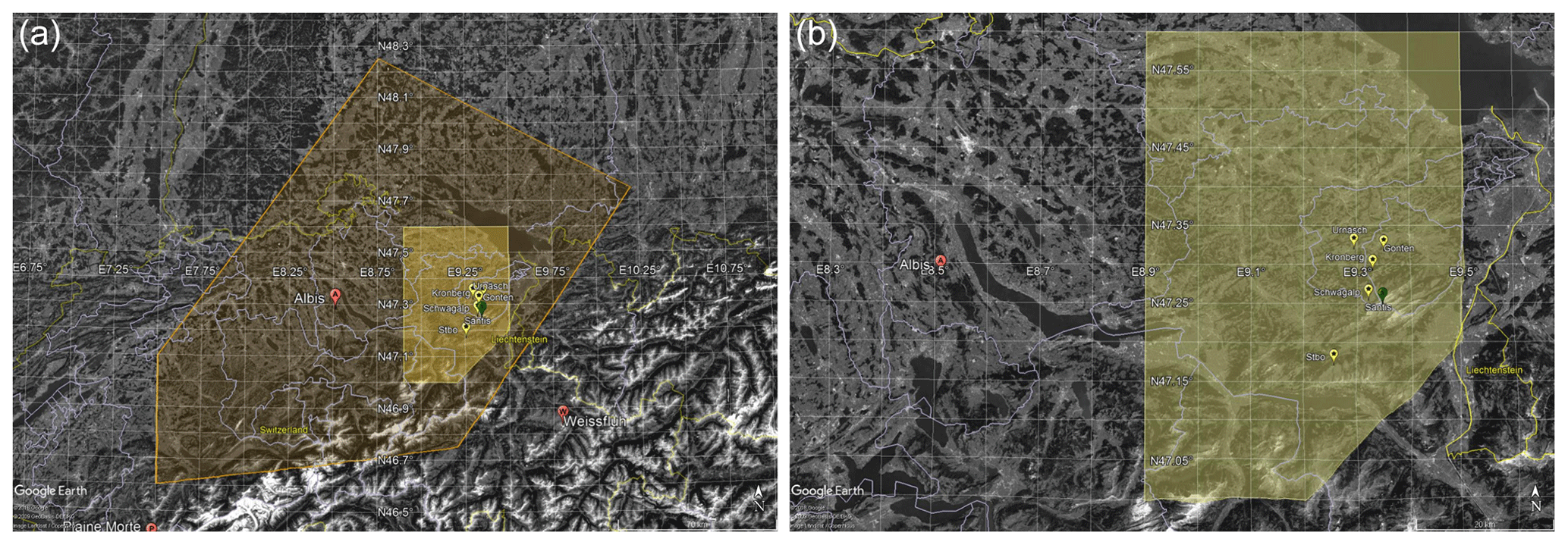
Figure 1(a) Approximate extent of the maximum area covered by the LMA (orange polygon). The yellow area shows the region with more comprehensive coverage. Radar positions are marked by red dots, while the position of the LMA sensors is marked by yellow dots. The Säntis tower is marked by a green dot. (b) Zoom over the best-covered area.
Since 15 July 2016, an EFM-100 field mill is installed 85 m from the tower to measure the electrostatic field. The system can detect lightning activity up to distances of about 40 km from the tower (Azadifar, 2017). In addition to this, an electric field measuring system comprised of a flat plate antenna and an analogue integrator with an overall operating frequency band between 30 Hz and 2 MHz is installed 14.7 km away from the Säntis tower (He et al., 2018).
2.1.2 Lightning mapping array
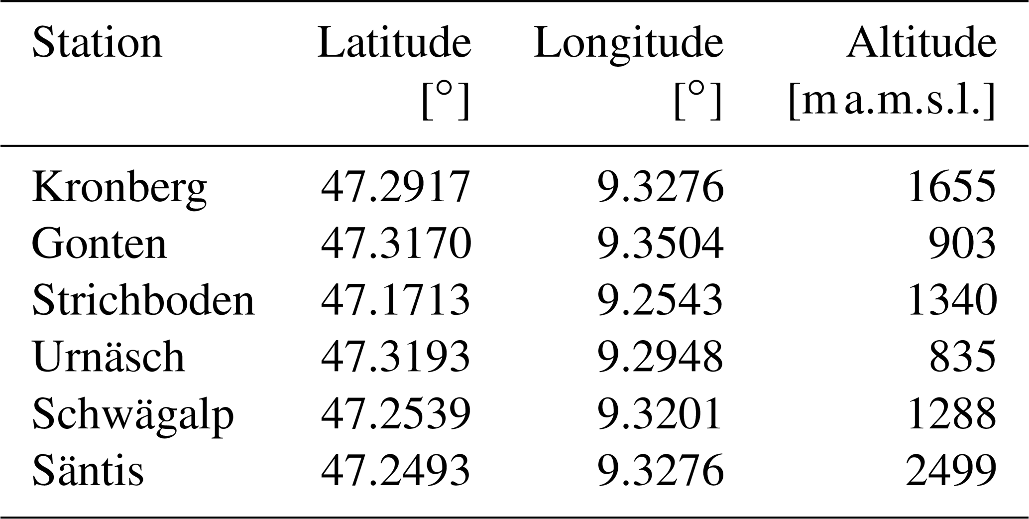
LRG owns and operates a 3-D LMA installed on a permanent basis at the lower part of the Ebro Valley, in Catalonia (van der Velde and Montanyà, 2013). The LMA network there consists of 12 VHF (60–66 MHz) sensors, some of which are mobile. For this campaign, 6 sensors were moved temporarily to locations in the area surrounding Säntis (see Table 1 and Fig. 1 for the locations). The network was operational from 29 June to 15 August 2017, although not all the sensors were operating during the entire period. The selection of the locations was made taking into consideration practical installation aspects such as accessibility, security, and reliable access to AC power and communication, as well as considerations of the magnitude of the local noise within the frequency band and the distance to the Säntis tower. In the end, the sensors were located in the vicinity of mobile phone base stations belonging to Swisscom and Swisscom Broadcast, which in the cases of the Gonten, Schwägalp and Säntis stations resulted in an increased noise level coming from the on-site telecommunications equipment. The Säntis station had the added challenge of being located indoors.
Each sensor measures the arrival times of the impulsive VHF radiation sources with an accuracy of 50 ns using a PC-based digitiser card coupled to a GPS receiver. The received signal is digitised and the peaks (within a 80 µs window) are time-tagged using the time derived from GPS receivers, which provide a timing pulse once per second (Rison et al., 1999). The timed data are stored on-site as well as transmitted over wireless modems to a central site for real time analysis and display. If at least four stations are able to measure the time of arrival of the radiation from a particular impulsive event, the three-dimensional position of the source region can be estimated since this is described by four unknowns (the three position coordinates, x, y, z, plus the exact time when the discharge occurred t). A redundancy in the number of stations observing the event allows for better accuracy and helps in filtering out noise spikes from other source types. After post-processing, individual sources deemed to be part of the same flash are clustered together and assigned a unique ID number (Fuchs et al., 2015). If the data point is not identified as belonging to any flash, it is assigned the ID number 0. A file with data from all the sources is generated each day. In this campaign, in order to account for the increased noisiness of the data and the poor visibility, a minimum of 10 detected VHF sources is required for a flash to be accepted.
Since the detection of the lightning strike requires direct line of sight of the source, LMAs observe mainly IC activity, mostly from negative leaders moving through regions of positive charge. However, weaker sources from positive leaders moving through negative charge regions are often detected. CG activity is often detected indirectly from stepped negative leaders or, less often, from negative dart leaders and sometimes positive leaders as well.
2.1.3 EUCLID lightning detection network
Operational detection of CG and IC activity is performed by the European Cooperation for Lightning Detection Network (EUCLID) (Schulz et al., 2016). The network uses various Vaisala sensors that detect low-frequency (1–350 kHz) electromagnetic signals and GPS receivers providing the time. The raw data are sent to a centralised location where they are processed and for each lightning strike the time of event, latitude and longitude of the impact point, and the current intensity and polarity are recorded. The EUCLID network has a high CG detection efficiency (on the order of 95 %) but a reduced IC detection efficiency, typically on the order of 50 %. The median accuracy is on the order of 100 m, although it may be worse in mountainous areas (Azadifar et al., 2015). The data available at MeteoSwiss is provided by Météorage and has a time resolution of 0.1 s.
2.2 Polarimetric weather radar data
MeteoSwiss owns and operates a network of five C-band Doppler polarimetric weather radars. The network was recently renewed within the project Rad4Alp, which was concluded in 2016 (Germann et al., 2015). The five systems have identical specifications and modes of operation. The scanning strategy consists of 20 horizontal scans with elevations ranging from −0.2 to 40∘ repeated every 5 min. The elevations are inter-leaved, every 2.5 min a half-volume of 10 elevations from top to bottom is concluded. A very short pulse of 0.5 µs is used to obtain data with a range resolution of 83.3 m with angular resolution of 1∘. In-phase and quadrature components of a signal (IQ) data are processed on-site using standard techniques (e.g. Doviak and Zrnic, 2006) to obtain the basic polarimetric moments, i.e. reflectivity (horizontal Zh and vertical Zv), differential reflectivity (Zdr), co-polar correlation coefficient (ρhv) and raw co-polar differential phase (ψdp), as well as Doppler moments. These basic moments are transmitted to a central server. The operational data processing involves a clutter detection using a sophisticated decision tree filter (DT-filter) and a reduction of the resolution to 500 m by averaging six consecutive gates (only the clutter-free ones). From the low-resolution polarimetric moments all subsequent products are generated. For the measurement campaign, data from the Albis radar (47.2843∘ N 8.5120∘ E, 938 ), situated 63 km west of the Säntis tower (see Fig. 1) were used.
2.2.1 Basic radar data processing
A specific non-operational processing was applied to radar data obtained in real time during the campaign. The processing was performed using the Python-based open-source software Pyrad/Py-ART (Figueras i Ventura et al., 2017). The first step was calculating the signal-to-noise ratio (SNR) of the horizontal channel using the estimated receiver noise from a high elevation angle (40 or 35∘). The SNR, together with the ratio between the horizontal and vertical channel receiver noise were used to minimise the effect of noise on ρhv (Gourley et al., 2006). Clutter identification was performed using a simple DT-filter based on the textures of Zh, Zdr, ρhv, and ψdp and the value of ρhv. Range gates identified as clutter-contaminated were removed from the analysis. ψdp was processed by first filtering out range gates with an SNR below 10 dB to reduce the influence of phase noise and then applying a double window moving median filter. The length of the windows was 1000 and 3000 m, respectively. The short window was applied in regions of high reflectivity (above 40 dBZ) while the long window was used elsewhere. The filtered differential phase (ϕdp) was used to compute the specific attenuation Ah using the ZPHI algorithm (Ryzhkov et al., 2014; Testud et al., 2000). Ah was estimated up to the freezing level height as determined by the temperature provided by the closest available run of the Numerical Weather Prediction (NWP) model COSMO-1 (see http://www.cosmo-model.org/, last access: 21 May 2019). From Ah, the specific differential attenuation Adp was derived. By integrating Ah (Adp) attenuation, the path integrated (differential) attenuation was obtained and this quantity was added to the (differential) reflectivity in order to correct for the precipitation-induced attenuation. In parallel to the attenuation correction, the specific differential phase (Kdp) was derived from ϕdp using the method described in Vulpiani et al. (2012).
Kdp, Zh, Zdr, ρhv and the temperature from the COSMO model were inputs of the semi-supervised hydrometeor classification described by Besic et al. (2016). The hydrometeor classification provides the following outputs: aggregates (AG), ice crystals (CR), light rain (LR), rimed particles (RP), rain (RN), vertically oriented ice crystals (VI), wet snow (WS), melting hail (MH), ice hail and high density graupel (IH), and no classification (no valid radar data, NC). An example of the output can be found in Fig. 11 of the aforementioned paper. It must be mentioned here that the category vertically oriented ice crystals is often misclassified. It is highly dependent on the Zdr value, with the assumption of Zdr being negative when the particles are vertically oriented. Unfortunately, at the C-band large values of Adp are not uncommon. Although Adp is corrected for, insufficient correction typically results in negative Zdr values at the far end of the ray. Therefore, the vertically oriented ice crystals category may contain a large proportion of regularly oriented ice crystals situated at range gates far away from the radar.
In addition to the dominant hydrometeor class, the MeteoSwiss hydrometeor classification algorithm also provides an estimation of the entropy (Besic et al., 2018). Such a quantity provides information about whether there is a clearly dominant hydrometeor type within the radar resolution volume (entropy 0) or if it is a heterogeneous mixture without any dominant hydrometeor type (entropy 1). Moreover, using the technique described in Besic et al. (2018), we are able to extract semi-quantitative information of the proportion of each hydrometeor type contained in the resolution volume.
At the end of the processing, high-resolution clutter-free volumes of attenuation-corrected Zh and Zdr, ρhv, Kdp, the model air temperature, the dominant hydrometeor type, the entropy, and the proportion of each hydrometeor type at each range gate were obtained. These parameters were used in the subsequent analysis.
2.2.2 Radar data along lightning trajectories
Within the radar data processing tool Pyrad, a lightning trajectory function has been implemented. This function reads the daily produced LMA lightning data and determines from them the time of the first and last VHF source detection. It then loops over all the radar volumes within this time interval and assigns to each VHF source the value of the polarimetric parameter in the range gate closest (both in time and space) to the source location. For each radar variable a file is generated containing the flash source time, the flash number, the value at the flash position and the mean, minimum and maximum of the cube formed by the neighbours.
2.2.3 Association of LMA flashes to EUCLID CG strokes
A two-step algorithm associates LMA flashes to corresponding EUCLID CG strokes. The first step looks for EUCLID CG strokes occurring during the propagation time of each LMA flash. A 0.1 s tolerance is added to the start and the end of the LMA flash since this is the time resolution of the EUCLID data available at MeteoSwiss. If EUCLID strokes have been found within the LMA flash duration, a second step looks at whether these EUCLID strokes are within the area covered by the LMA flash. The LMA flash area is defined as the minimum oriented rectangle that contains all the VHF sources of the flash projected to the ground. The minimum area of this rectangle is set to 25 km2, which is considered a reasonable area to look for in case of flashes with reduced horizontal extent. A scaling factor of 1.2 is applied to each dimension of the rectangle if its area is larger than the minimum area to account for the fact that the flash may still propagate horizontally below the LMA detectable altitude. If EUCLID strokes are present within the LMA flash area, the LMA flash data are saved in a separate file. This process can be performed to associate LMA flashes to all, only positive or only negative CG EUCLID strokes. A separate process gets the complementary data, i.e. LMA flashes without associated CG EUCLID strokes, by comparing the file with all the flash data with the resultant filtered data file.
3.1 Data availability and coverage
The LMA was installed in the Säntis area between 29 June and 15 August 2017. On half of the days that the campaign lasted (24 out of 48) some lightning activity was registered in the area covered by the LMA of the EUCLID network. Of these, on 15 d lightning activity was registered within 2 km from the Säntis tower. On 10 of these, direct strikes to the tower were also registered by the in situ sensors. According to the operational MeteoSwiss probability of hail (POH) algorithm, hail with a probability above 90 % was present somewhere within the domain on 11 d. On 6 of these days hail was detected within 20 km of the Säntis tower. Figure 2 provides an overview of the relevant events during the campaign. For our analysis, we have focused on events that produced lightning in the immediate proximity of the tower. Of these, 22, 24 and 25 July were excluded because fewer than five LMA stations were operational. The data from 5, 8, 9 and 15 August were excluded as well because, although enough stations were operating, for reasons still under investigation the data quality was poor. Some characteristics of the events with lightning in the vicinity of the Säntis tower can be seen in Table 2. During the 8 d where LMA data were analysed, a total of 1 586 394 VHF sources, corresponding to 12 062 flashes, were detected (i.e. 132 VHF sources per flash). Almost half of them were detected on the first of August alone.
Table 2Analysed days and some of their general characteristics.

NA: not available
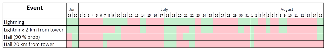
Figure 2Overview of relevant events within the LMA reduced domain occurred during the 2017 campaign. Hail probability is derived from the POH radar product. Occurrence of relevant events is marked in green.
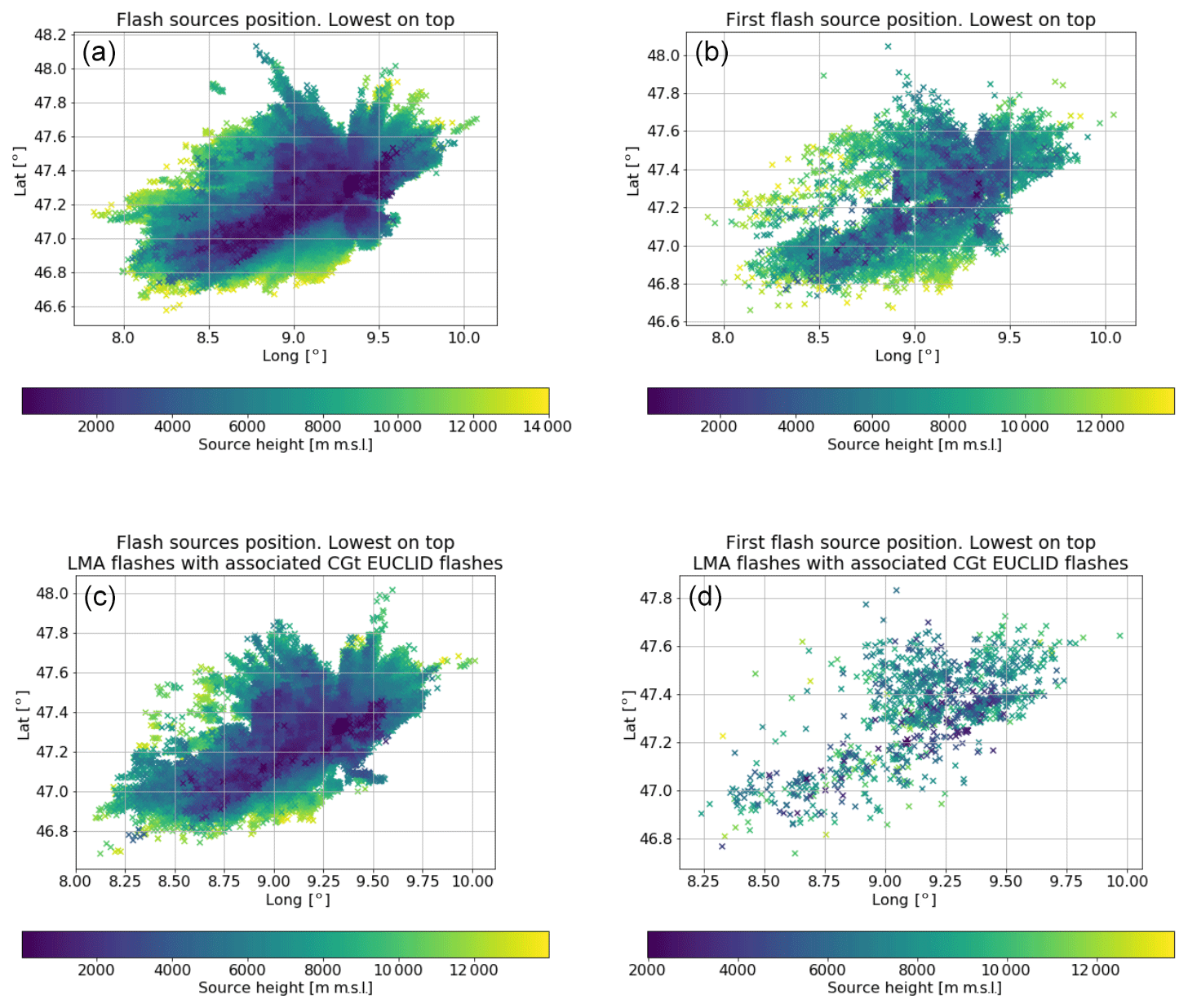
Figure 3Position of detected VHF sources for the days examined. (a, c) All VHF sources. (b, d) Only the first sources of each flash. (a, b) All data. (c, d) Flashes with associated EUCLID CG strokes.
Figure 3a plots the position of all the LMA detected VHF sources during the days analysed. Each cross in the plot is a detected LMA VHF source. The data have been colour-coded by estimated altitude with lowest altitude in dark blue. The lowest-altitude VHF sources are plotted on top. As the plot shows, the data are distributed over a broad surface oriented from southwest to northeast, which was the moving direction of most of the convective cells during the period analysed. It is also apparent that the coverage of the LMA network is uneven. There is a section in the south, oriented from southwest to northeast, where the minimum altitude at which data are detected is much higher due to blockage from the Alps. Likewise, there is a gradual loss of detectability the further one moves away from the centre of the network. Since the number of operational sensors varied between five and six during the days examined and the malfunctioning sensor was not always the same, the actual detectability varies between days. Nevertheless, the area surrounding Säntis appears to be reasonably well covered. Figure 3b plots the position of the first LMA detected VHF source of each flash during the days analysed. It can be seen that they have an uneven distribution with a band with high density of flashes to the south and a second band with a lower flash density further north. However, this seems to be associated more to the path of individual storms than to specific detectability issues.
3.2 General data analysis
This section discusses the bluish areas of the histograms in Figs. 4–8 that provide a general overview of all the data sources collected during the days analysed. It should be noticed that in all the histograms presented in this paper, the values outside of the histogram range are added to the bins at the extremes, e.g. the last bin in the histograms in Fig. 4a include all the values above 900 ms.
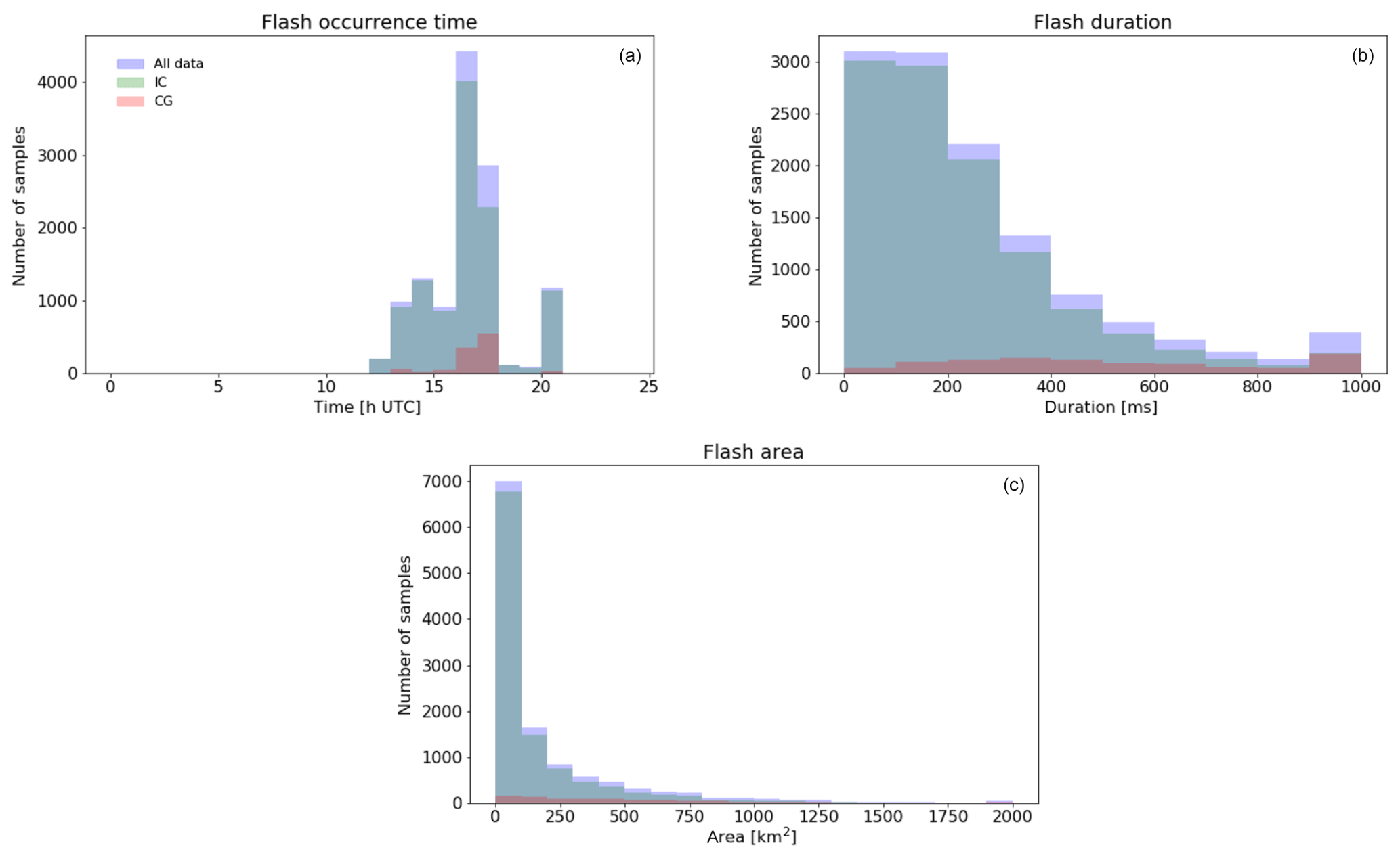
Figure 4Distribution of the LMA flashes for all days analysed: (a) time of occurrence, (b) duration, (c) 2-D projection area over the day for all days analysed. Bluish area: all data. Greenish area: flashes without associated EUCLID CG strokes. Reddish area: flashes with associated EUCLID CG strokes. Note that the values outside of the histogram range are added to the bins at the extremes.
Concerning the distribution of the flashes over the day (see Fig. 4a), they are concentrated in the afternoon. The first flashes are detected at 10:00 UTC and the last at 21:00 UTC, with a clear peak at 16:00 UTC. Obviously, with so few events, the distribution is highly dependent on the severity and time of occurrence of the individual events but it seems probable that in the study area there is a diurnal cycle with a peak at mid-afternoon during the summer months. Figure 4b shows the distribution of the duration of the flashes. For our purposes we define the flash duration as the time difference between the first and the last VHF source identified as belonging to a single flash. As it can be seen it has an exponential distribution. A total of 51 % of flashes have a duration of up to 200 ms. On the other hand, 3 % of flashes have a duration of more than 900 ms. The flash area (see Fig. 4 bottom panel) also follows a marked exponential distribution with more than half (58 %) covering an area of less than 100 km2. There are few flashes though (0.4 %) that cover an area of more than 1900 km2.
Figure 5 shows histograms of the power of the VHF sources detected by the LMA. In Fig. 5a, all sources are shown while in Fig. 5b only the first detected source for each flash (which we consider a proxy for flash origin) is shown. The histogram exhibits a Gaussian-like shape with median of 18.5 dBm. Detected sources had power ranging from −16 to 46 dBm. The sources power at the origin also has a Gaussian-like shape but has increased power. The median in this case is 20.5 dBm.
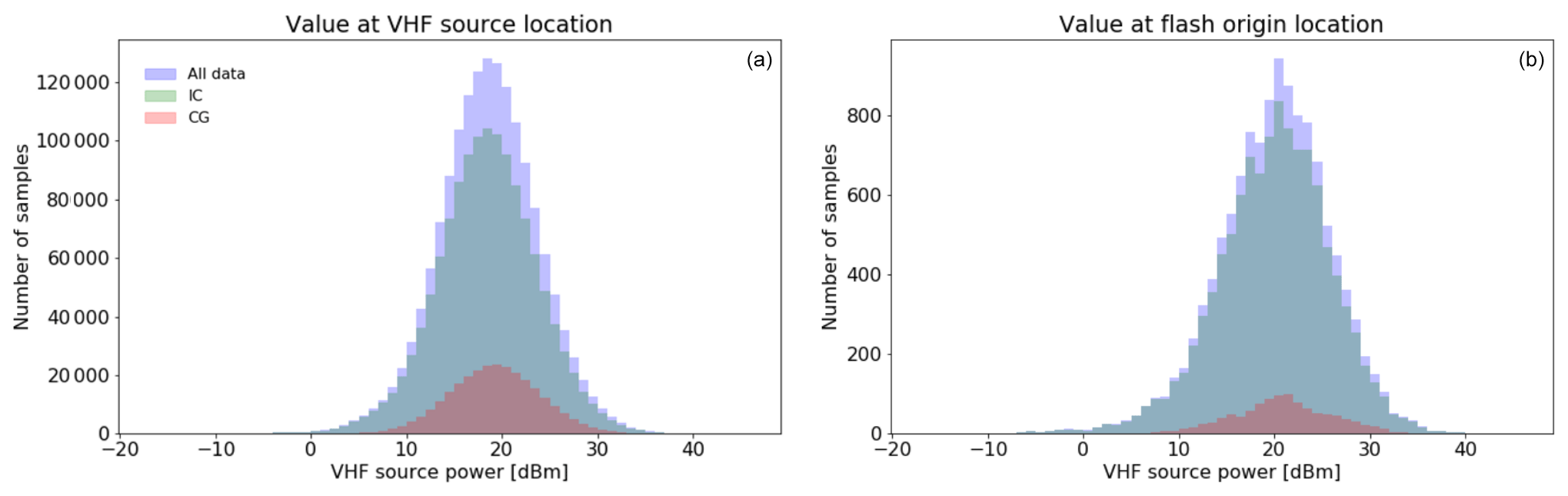
Figure 5Histogram of VHF sources power for all days analysed. (a) All sources. (b) Only the first sources of each flash. Bluish area: all data. Greenish area: flashes without associated EUCLID CG strokes. Reddish area: flashes with associated EUCLID CG strokes. Note that the values outside of the histogram range are added to the bins at the extremes.
Table 3Number of VHF sources (flashes) detected and percentage of each dominant hydrometeor type at the location of each flash type.
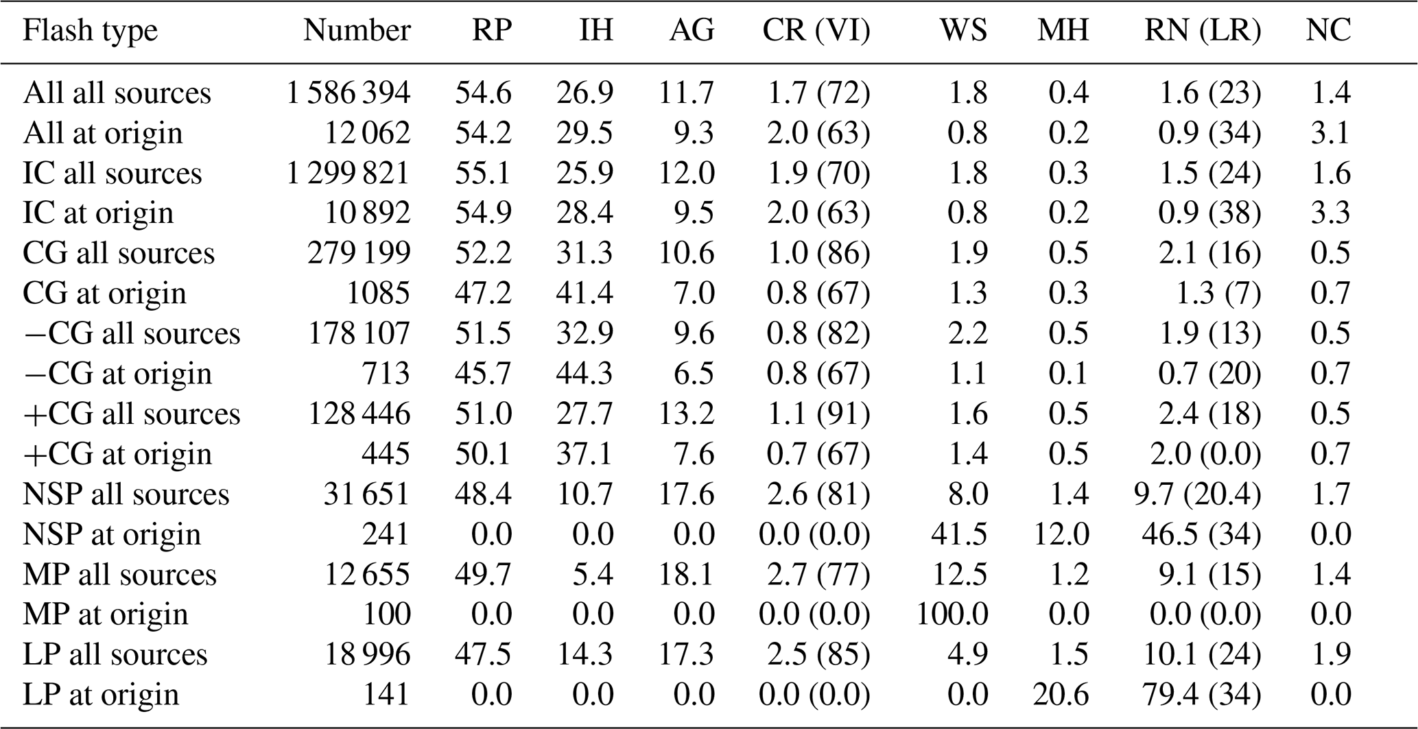
Figure 6a and b show histograms of the altitude of the VHF sources detected by the LMA. It can be seen that, whereas the altitude histogram of the flash origin has a Gaussian-like shape with a mode of 8600 and median of 8200 (Fig. 6b), when all sources are considered the histogram has a bimodal shape with two distinct peaks: the main one at 7400 and a secondary one at 4000 (Fig. 6a). This suggests that most of the IC lightning activity is generated at the higher part of the clouds with the majority of the flashes roughly propagating horizontally but a significant proportion descending into lower layers. This observation is further confirmed by Fig. 6c and d in which the temperature at the location of each lightning source, obtained from the COSMO-1 NWP model, can be seen. Indeed, the vast majority of the sources are detected at freezing temperatures. The median temperature for all sources is −20∘C, while the lightning origin is at −25∘C.
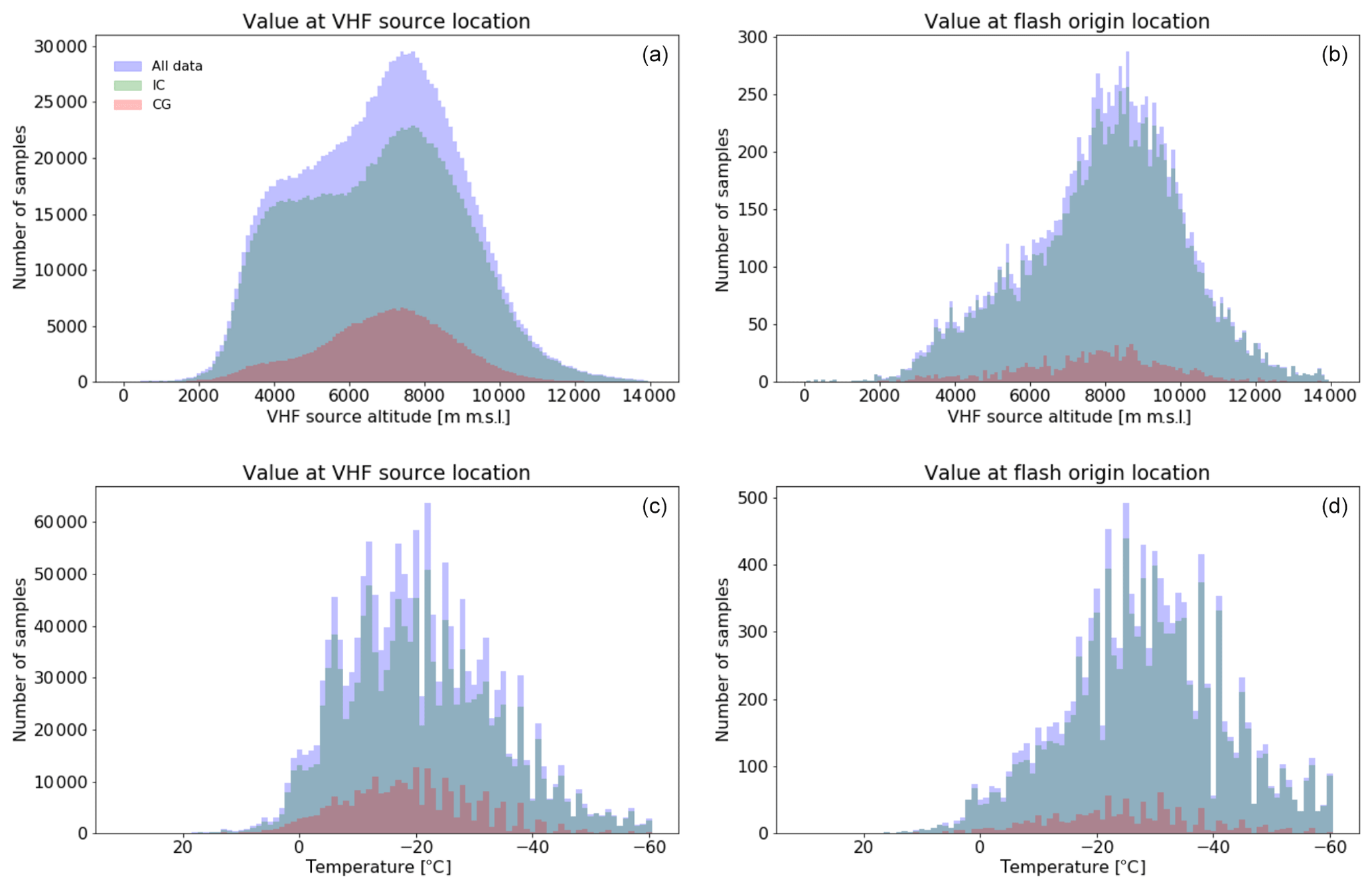
Figure 6Histogram during all days analysed of (a) VHF sources altitude. (b) Only the first sources of each flash altitude. (c) The model air temperature of all sources. (d) The first source's model air temperature. Bluish area: all data. Greenish area: flashes without associated EUCLID CG strokes. Reddish area: flashes with associated EUCLID CG strokes. Note that the values outside of the histogram range are added to the bins at the extremes.
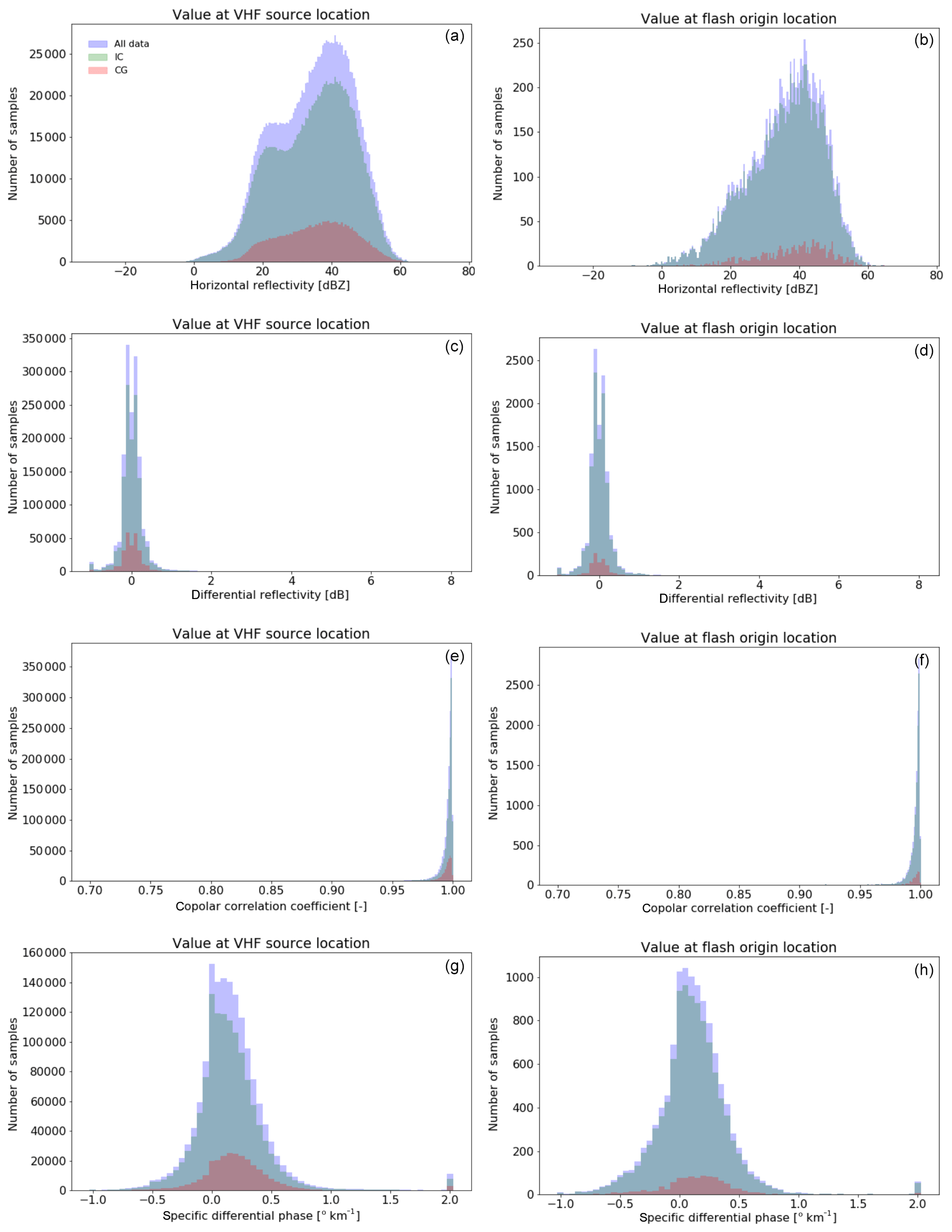
Figure 7Histogram during all days analysed of, from top to bottom, Zh, Zdr, ρhv and Kdp. (a, c, e, g) All sources. (b, d, f, h) The first source only. Bluish area: all data. Greenish area: flashes without associated EUCLID CG strokes. Reddish area: flashes with associated EUCLID CG strokes. Note that the values outside of the histogram range are added to the bins at the extremes.
The reflectivity data (Fig. 7a and b) of all sources show a bimodal distribution with a main peak at 41 dBZ and a secondary peak at 25 dBZ. Interestingly, when looking only at the first source the main peak is maintained (at 41.5 dBZ), but the secondary peak is barely visible. It is worth noting that a similar behaviour was observed when looking at the altitude of the VHF sources (Fig. 6). We think that this is due to the tendency of flashes to preferentially propagate horizontally through layers with a high density of charge. The 2-D histogram of altitude–reflectivity and the analysis of individual storms (not shown) show that there are three areas with a higher density of flashes. Indeed, most sources are concentrated in an area with roughly the same altitude and reflectivity as the flash origin while two other less dense preferential areas appear: one at roughly the same altitude but with lower reflectivity and another with similar reflectivity values but at another altitude. Our interpretation is that flashes are likely to either propagate horizontally at similar altitudes to where they are generated, sometimes extending beyond the convective core (hence the lower reflectivity), or move to a lower layer within the convective core. The Zdr data (upper-middle panels) exhibit a similar Gaussian-like shape both when all sources are considered and when only the first source is considered. In both cases the distribution is centred around 0 but with very long tails. ρhv data (lower middle panels) have a log-normal shape with most values well above 0.99. The mode is 0.9990 both when considering all sources and when only considering the first one. Kdp values (lowermost panels) are centred at 0, but they are noticeably skewed towards positive values.
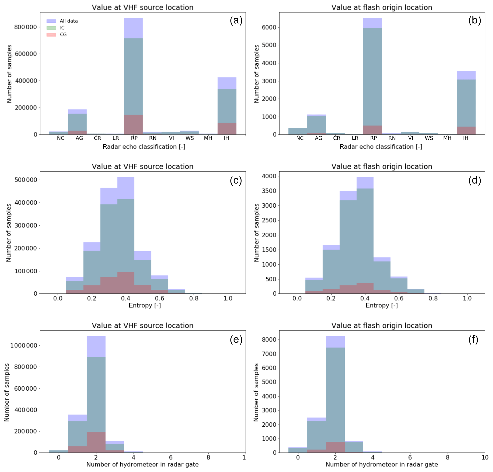
Figure 8Histogram during all days analysed of, from top to bottom, the dominant hydrometeor at the radar gate collocated with the VHF source position, the hydrometeor-classification-derived entropy at the radar gate collocated with the VHF source position and the number of hydrometeor types with a significant presence at the radar gate collocated with the VHF source position. (a, c, e) All sources. (b, d, f) The first source only. Bluish area: all data. Greenish area: flashes without associated EUCLID CG strokes. Reddish area: flashes with associated EUCLID CG strokes. Note that the values outside of the histogram range are added to the bins at the extremes.
Figure 8a and b show histograms of the dominant hydrometeor at the location of the VHF sources. This information is tabulated in Table 3. As it can be seen, the large majority of the sources are produced in areas of rimed particles or dry hail. When considering only the first sources, the proportions of these species are essentially maintained, with a slight increase in the solid hail proportion. The other classes with significant VHF sources are dry snow and ice crystals. A high percentage of ice crystals are labelled as vertically aligned ice crystals, which is indicative that those are ice crystals situated at the far end of the radar, i.e. high up in the atmosphere. Again, similar proportions are encountered when examining only the first sources, but there is a decrease in vertically aligned ice crystals, which may indicate that flashes are less likely to originate at the very top of the cloud. The percentage of VHF sources detected in the mixed-phase or liquid-phase layers (i.e. wet snow, melting hail or rain) is marginal, a mere 3.8 %. A total of 94.9 % of the flashes detected originated at the solid-phase region of the precipitating systems whereas only 2.0 % originated in the mixed-phase or liquid-phase regions of the precipitating systems. A total of 3.1 % have an origin in regions where no radar echo was detected but from examining the location (not shown) it can be inferred that for the most part they correspond to the solid-phase region.
Figure 8c and d show histograms of the entropy of the hydrometeor classification at the location of the VHF sources. It is evident from the graph that the entropy tends to be rather high, with values on the order of 0.3 and 0.4 dominating the distribution and representing 62.4 % of all the VHF sources and 64 % of all the flash origins where radar data were present. Indeed, when looking at how many hydrometeor types have a significant presence within the radar gates collocated with VHF sources (more than 10 % contribution to the hydrometeor proportions) (see Fig. 8e and f), it turns out that in a large majority of them there is more than one hydrometeor type and up to a maximum of 6. A total of 69 % are composed of two hydrometeor types, while only 22 % contain one single dominant hydrometeor. If looking at the flash origin only, the number of gates containing only one hydrometeor type decreases further by one point (21 %).
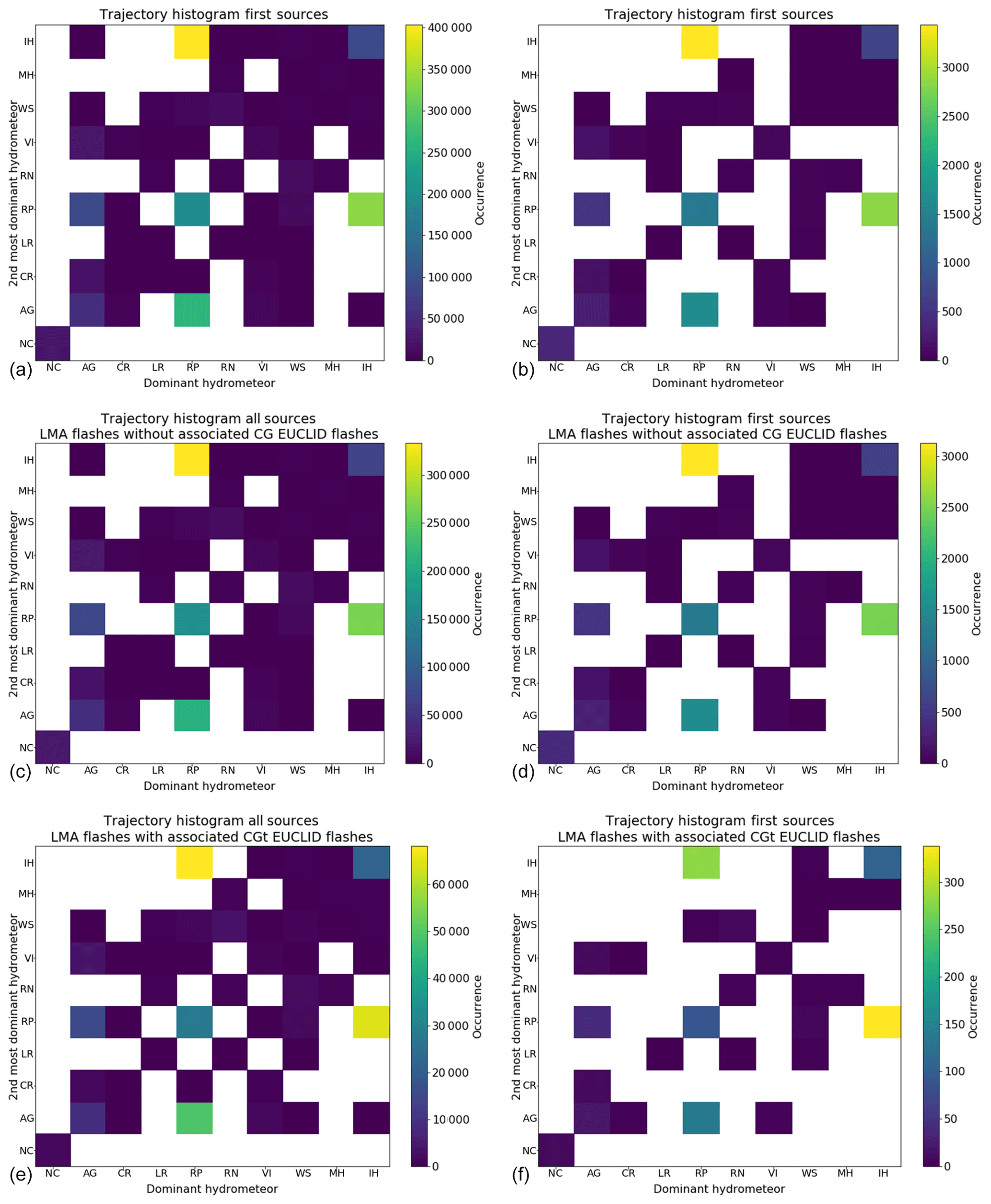
Figure 9Two-dimensional histogram of the type of the most-dominant and second most-dominant hydrometeor at the radar gate collocated with the VHF source position. From top to bottom: all data, flashes without associated EUCLID CG strokes, flashes with associated EUCLID CG strokes. (a, c, e) All VHF sources in the flash. (b, d, f) Only the first VHF sources.
Figure 9a and b show 2-D histograms of the most-dominant and second most-dominant hydrometeors. The most likely combination of hydrometeors in the presence of VHF sources by far is a combination of rimed particles as the most-dominant type and solid hail as the second most common. The second most likely is the combination of solid hail as the most-dominant type and rimed particles as the second most common. The third is a combination of rimed particles as the most dominant and aggregates as the second most common, while the fourth is rimed particles as single dominant hydrometeor. When focusing on the flash origin this ranking is essentially maintained but the likelihood of a combination of rimed particles and aggregates decreases. It seems clear from these results that lightning tends to originate in areas with an important presence of rimed particles or solid hail.
3.3 Characteristics of the flashes without associated EUCLID cloud-to-ground strokes
Here we analyse the characteristics of flashes without associated EUCLID CG strokes, which we use as a proxy for IC flashes. This section discusses the greenish area of the histograms in Figs. 4 to 8. A total of 90.30 % of the total flashes (10 892) correspond to this category. Those flashes contain 81.94 % of the total detected sources (1 299 821). The fact that flashes without associated EUCLID CG strokes have fewer sources per flash (119 compared to 132) may be an indicator that this type of flash is more short-lived and has a simpler structure.
Since a very large proportion of flashes are IC flashes, their characteristics do not differ significantly from the general analysis performed in the previous subsection. The VHF source power distribution (see Fig. 5) is very similar. The VHF source altitude (Fig. 6) and the reflectivity distributions (Fig. 7a) have a more marked bimodality.
The distribution of the values of the hydrometeor classification (see Fig. 8a and b and Table 3) is essentially the same as when all data are considered. As is the case with all the data, the entropy is quite high (see Fig. 8c and d), and most of the radar gates where VHF sources are located contain more than one hydrometeor type (see Fig. 8e and f). Rimed particles or solid hailstones are present in most regions where the flashes propagate (see Fig. 9c and d).
3.4 Characteristics of the flashes with associated EUCLID cloud-to-ground strokes
Here we analyse the characteristics of flashes that have associated EUCLID CG strokes, referred to here as CG flashes. This section discusses the reddish area of the histograms in Figs. 4 to 8. This category contains a total of 1085 flashes, which correspond to 9.0% of the total. Those flashes contain 17.60 % of all the sources detected during the days analysed (279 199). On average the CG flashes during the campaign contain 257 sources. This would suggest that those flashes have a more complex structure than the IC flashes. Figure 3c and d show the spatial distribution of all the VHF sources of these flashes (left) and the first VHF source of each flash (right). The spatial distribution of all VHF sources approximately covers the same area that was covered by all data. However, the density of the flash origin is much lower and there are few detections in the northeast band of lightning activity, suggesting that individual storms have a varying ratio of CG to IC flashes. That is further confirmed by looking at the time of occurrence of the flashes (see Fig. 4a), since the shape of the distribution changes significantly. The flash duration distribution (Fig. 4b) does not follow an exponential distribution anymore but has a mode of 350 ms, and a large number of flashes (17 %) have a duration of more than 900 ms. The area covered by the flashes (Fig. 4) also tends to be larger. Only 15 % of the flashes cover an area of less than 200 km2 and 3 % of the flashes cover an area of more than 1900 km2.
In terms of source power (Fig. 5), CG flashes exhibit similar characteristics to those of the global analysis. Their histogram again has a Gaussian-like shape with the median a bit higher (19.5 dBm). When only the first sources are considered the median is the same as in the global analysis, 20.5 dBm. Regarding the altitude of the VHF sources, there are remarkable differences (see Fig. 6a and b) to the global data. When all sources are considered, the histogram exhibits a Gaussian-like distribution but skewed towards lower altitudes with a median of 7000 and a mode of 7400 . When only considering the origin of the flashes, the histogram has an almost uniform-like distribution with a mode of 8700 and median of 7900 . There is a 300 m difference between the median of CG flashes with respect to the global data, which may indicate that those flashes are more likely to be generated at lower altitude. This is backed also by the fact that the median temperature at the flash origin (Fig. 6 bottom right panel) is −25∘C compared to the −28∘C of the global data.
In terms of distribution, the polarimetric variables show subtle differences with respect to the global data (see Fig. 7). When all sources are considered, the secondary peak in the reflectivity distribution is almost unnoticeable and the mode is lower (39 dBZ) and the median higher, 36.5 dBZ. When only the origin is taken into account, both the median and the mode are decisively larger (40 and 44 dBZ, respectively). The Zdr distribution is similar but with comparatively fatter tails. ρhv has slightly lower median (0.996 both when all sources are considered and when only the first source is considered). The Kdp distribution is very similar but shifted towards higher values, particularly for the source origin, where the median has moved to 0.15.
Although the general distribution is maintained with respect to the global data analysis, the proportions of each hydrometeor class are slightly different (see Fig. 8a and b and Table 3). When considering all VHF sources in the solid phase, their proportion decreases slightly but not dramatically. As would be expected, the percentage of sources transiting through the rain medium is remarkably higher with respect to IC flashes. When looking at the origin of the flashes, the percentages of flashes originating in the solid phase decreases with respect to the global data. It is interesting to notice that there is a marked increase in flashes having their origin in solid hail regions and a decrease in flashes produced in the dry snow or ice crystals regions with respect to the global data. The percentage of VHF sources where hydrometeor classification could not be performed is lower than in the global analysis, which corroborates the statement that non-classified data are located mostly at high altitude.
As was the case with the global data, the entropy of the hydrometeor classification is rather high, with a large percentage of VHF sources located in regions with entropy on the order of 0.3–0.4 (see Fig. 8c and d). Again, flashes are more likely to be generated and propagate in areas where at least two hydrometeor types are present in significant proportions (see Fig. 8e and f).
Figure 9e and f show 2-D histograms of the most-dominant and second most-dominant hydrometeors for sources associated with EUCLID CG strokes. When looking at all sources (Fig. 9e) the distribution is rather similar to the global data. The main difference is that the combination of solid hail as the most dominant and rimed particles as the second most dominant has a comparatively higher weight. However, when looking at the flash origin (Fig. 9f) the mentioned combination becomes the most likely.
LMA flashes stratified by associated positive and negative CG activity
In this subsection we further stratify the data into flashes associated with negative EUCLID CG strokes (hereby −CG flashes) and flashes associated with positive EUCLID CG strokes (hereby +CG flashes). This section discusses the histograms presented in Figs. 10–13. In those figures the greenish area of the histograms correspond to −CG flashes while the reddish area of the histograms correspond to +CG flashes.

Figure 10Distribution of the flashes for all days analysed: (a) time of occurrence, (b) duration and (c) 2-D projection area over the day for all days analysed. (d) Number of detected EUCLID CG strokes per LMA flash. Bluish area: all flashes with associated EUCLID CG strokes. Greenish area: flashes with associated EUCLID −CG strokes. Reddish area: flashes with associated EUCLID +CG strokes. Note that the values outside of the histogram range are added to the bins at the extremes.
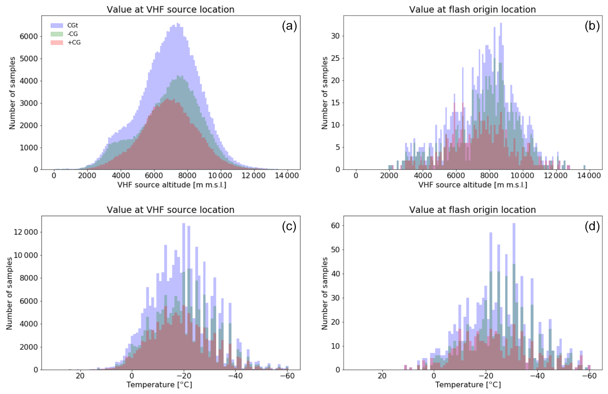
Figure 11Histogram during all days analysed of (a) VHF sources altitude, (b) only the first sources of each flash altitude, (c) all sources model air temperature and (d) the first source's model air temperature. Bluish area: all flashes with associated EUCLID CG strokes. Greenish area: flashes with associated EUCLID −CG strokes. Reddish area: flashes with associated EUCLID +CG strokes. Note that the values outside of the histogram range are added to the bins at the extremes.
There are 713 −CG flashes and 445 +CG flashes detected in the dataset. It should be noted that of the total CG flashes, 73 have both positive and negative CG strokes. Although the existence of bipolar flashes has been documented in the past, at this point we believe that this is mainly due to the limitations in the technique used to stratify the flashes. The necessary tolerance in time and space to associate multiple strokes into flashes may have resulted in the misattribution of strokes for flashes that are very close in time and/or space. In any case, the proportion of +CG flashes with respect to the total number of CG flashes (41 %) is significantly higher than that observed on the Säntis tower over a 2 year period (15 %) (Romero et al., 2013). That is due to the fact that on 3 out of the 8 analysed days (10 and 19 July and 1 August), the proportion of +CG flashes is abnormally high (see Table 2). The percentage of +CG flashes on 19 July (72.6 %) is particularly noteworthy. On that day, large swathes of terrain south of the Säntis tower were affected by hail according to the POH algorithm. There was also extensive hail recorded on 1 August. A higher proportion of +CG flashes have been linked to severe hail-bearing storms in past studies (see the introduction of Pineda et al., 2016, for a summary). The −CG flashes have a total of 178 107 VHF sources while +CG flashes have 128 446 VHF sources, thus +CG flashes have a more complex structure, with an average of 289 sources per flash with respect to the 250 sources associated with −CG flashes.
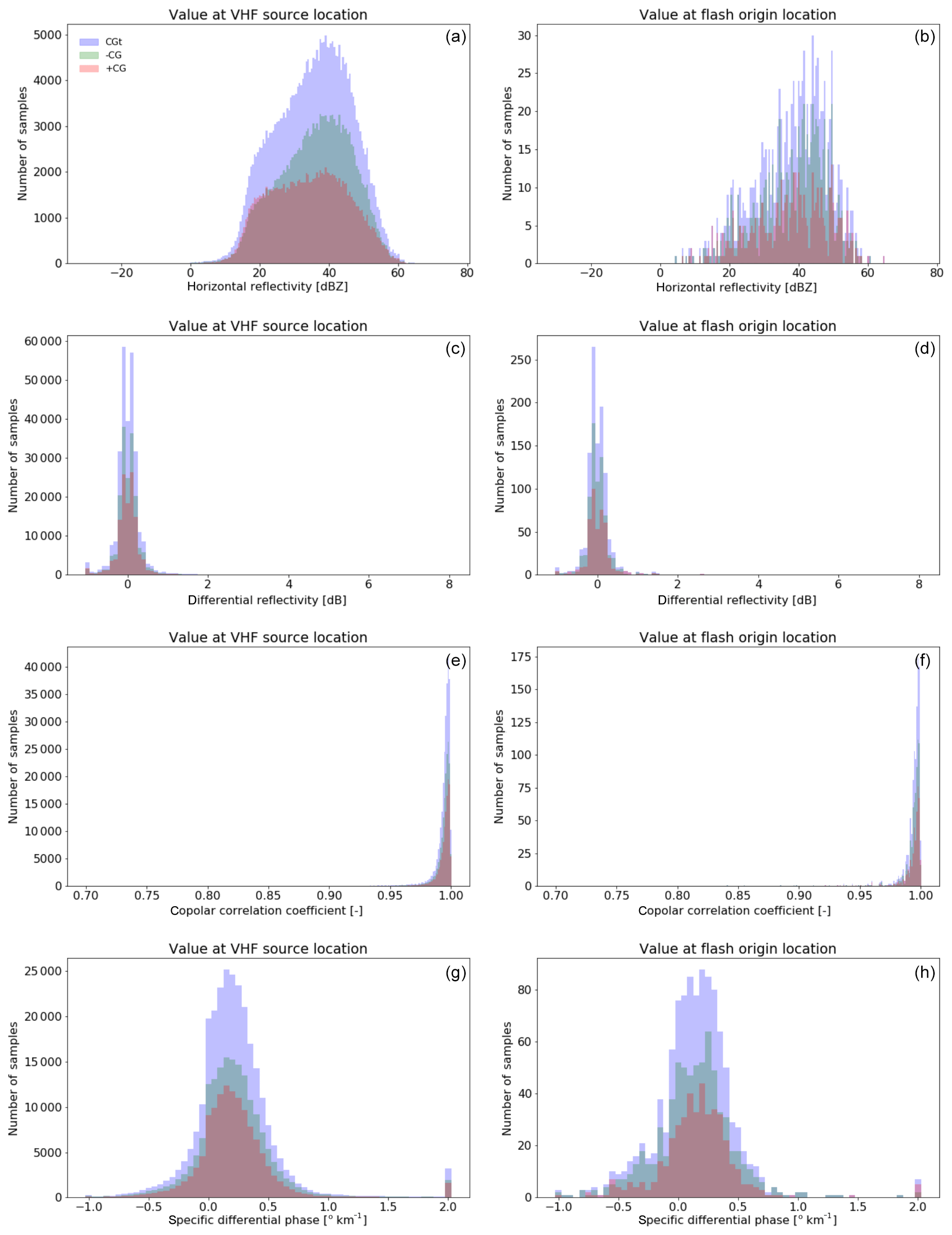
Figure 12Histogram during all days analysed of from top to bottom, Zh, Zdr, ρhv and Kdp. (a, c, e, g) All sources. (b, d, f, h) The first source only. Bluish area: all flashes with associated EUCLID CG strokes. Greenish area: flashes with associated EUCLID −CG strokes. Reddish area: flashes with associated EUCLID +CG strokes. Note that the values outside of the histogram range are added to the bins at the extremes.
Regarding the time of occurrence (see Fig. 10a), for both types of CG flashes there is a well-defined peak of occurrence between 16:00 and 18:00. However, while the number of −CG and +CG flashes occurring between 16:00 and 17:00 is roughly the same, between 17:00 and 18:00 the number of −CG flashes is double that of +CG flashes. This indicates that individual storms have a preference to produce either one type of flash or the other. The flash duration distribution (Fig. 10b) is very similar for both −CG and +CG flashes but +CG flashes tend to cover a larger area (Fig. 10c). Indeed the mode and the median of the +CG flashes area coverage is 450 and 650 km2, respectively, while that of the −CG flashes is 50 and 350 km2. Figure 10d shows the distribution of number of EUCLID CG strokes per LMA flash, i.e. its multiplicity. +CG flashes are mostly associated with a single EUCLID +CG stroke whereas −CG flashes are more likely to have several EUCLID −CG detections associated with them. The maximum number of EUCLID strokes detected for −CG flashes is 20 while for +CG flashes it is just 5.
In terms of source power (not shown), when looking at all VHF sources the distribution is very similar for both +CG flashes and −CG flashes and the median value is the same, 19.5 dBm. However, when looking at the first source the median power of +CG flashes is larger (21.5 dBm compared to 20.5 dBm).
Regarding the altitude of the VHF sources, there are remarkable differences between the two CG flash types (see Fig. 11a and b). −CG flashes exhibit a bimodal distribution with a peak at 7400 and another one at roughly 4000 . By contrast, +CG flashes have a Gaussian-like distribution with median value 6900 . When looking at the flash origin the contrast is even more marked. +CG flashes have a median altitude of 7500 , while −CG flashes have a larger median altitude of 8000 . Looking at the temperature data from the COSMO model (see Fig. 11c and d) we again observe a modest decrease in median value when all sources are considered from −CG flashes to +CG flashes (−19 to −18∘C) but a larger decrease when focusing on the flash origin (from −26 to −22∘C). Therefore, it seems clear +CG flashes tend to have an origin at lower levels in the precipitating system.
In terms of the distribution of the polarimetric variables (see Fig. 12), some minor differences can also be noticed. The reflectivity distribution of −CG flashes has a Gaussian-like shape, although skewed towards lower values, with median 37 dBZ, while +CG flashes have an almost uniform distribution with median value 34.5 dBZ when all sources are considered. When only the first sources are considered, the median is 40.5 dBZ for −CG flashes and 39 dBZ for +CG flashes. The other polarimetric variables have very similar distributions.
Focusing on the dominant hydrometeor types at each flash location (see Table 3) it is worth highlighting that a higher percentage of +CG flashes originate in the liquid-phase region than the corresponding percentage of −CG flashes (0.8 %). Also worth noting is the fact that a larger percentage of −CG flashes have an origin in regions where solid hail is the dominant particle with respect to +CG flashes. Having said that, as has been the case throughout all the data analysis, the entropy of the hydrometeor classification is rather high (0.4 mode), and most of the radar gates contain two or more hydrometeor types in significant proportions.
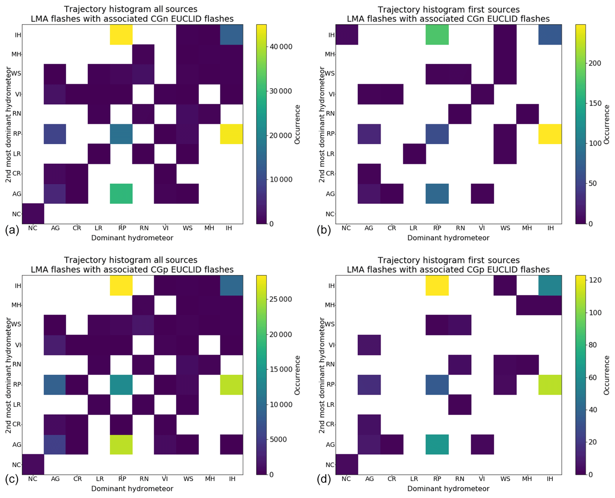
Figure 132-D histogram of the type of the most-dominant and second most-dominant hydrometeor at the radar gate collocated with the VHF source position. From top to bottom: all flashes with associated EUCLID CG data, flashes with associated EUCLID −CG strokes, flashes with associated EUCLID +CG strokes. (a, c) All VHF sources in the flash (b, d) and only the first VHF sources.
Figure 13 examines the most likely combination of hydrometeors at the location of the VHF sources. When looking at all sources, the most likely combinations for −CG flashes are solid hail and rimed particles, regardless of the dominant type, followed by a combination of rimed particles as the most dominant and aggregates as the second most common. When looking at the flash origin, the most likely combination is clearly dominant solid hail and rimed particles as the second most-dominant hydrometeor followed by rimed particles as the most dominant and solid hail as the second most dominant. When looking at +CG flashes the distribution is similar but there are some significant differences. The most likely combination when looking at all VHF sources clearly becomes rimed particles as the most dominant and solid hail as the second most dominant. In second place with similar percentages there is solid hail as the most dominant and rimed particles as the second most dominant and rimed particles as the most dominant and aggregates as the second most dominant. When looking at the flash origin, the most likely combination is rimed particles as the most dominant and solid hail as the second most dominant followed by solid hail as the most dominant and rimed particles as the second most dominant. A significant percentage of flashes have an origin in areas where rimed particles are dominant but aggregates are the second most dominant and in areas where the radar volume essentially contains solid hail.
3.5 Characteristics of the flashes with an origin in the liquid or mixed-phase regions
Here we focus our attention on LMA flashes with an origin in the liquid or mixed-phase regions. The reason for that is that those flashes are more likely to be of the upward lightning type. For our classification we have considered flashes whose first VHF source was in areas where the dominant hydrometeor was light rain, rain, melting hail or wet snow as belonging to the mixed-phase or liquid-phase regions . Flashes located in regions of wet snow are considered to have an origin in the mixed phase while flashes with sources in light rain, rain or melting hail are considered to have an origin in the liquid-phase region. This section discusses the histograms presented in Figs. 15 to 19. In those figures, the bluish area of the histogram corresponds to flashes with an origin in either the mixed-phase or liquid-phase regions, the greenish area of the histograms corresponds to flashes with an origin in the mixed-phase regions and the reddish area of the histograms correspond to flashes with an origin in the liquid phase. In the following we will call flashes with an origin in the liquid-phase (LP) flashes, flashes with an origin in the mixed-phase (MP) classes and flashes with an origin either in the mixed-phase or the liquid-phase non-solid-phase (NSP) flashes.
There are only 241 NSP flashes in the dataset. These flashes generated a total of 31 651 VHF sources. Of those, 100 are MP flashes (with 12 655 VHF sources) and 141 are LP flashes (with 18 996 sources). Regarding their position, Fig. 14 shows that they are mostly distributed in a narrow area going from southwest to northeast in line with the direction of the Alps. It is interesting to notice that a higher concentration of flash origins can be seen at the location of the Säntis tower and at another location south of it that we have identified as the Gamsberg area. This backs our assumption that a large percentage of those flashes have origins on the ground.
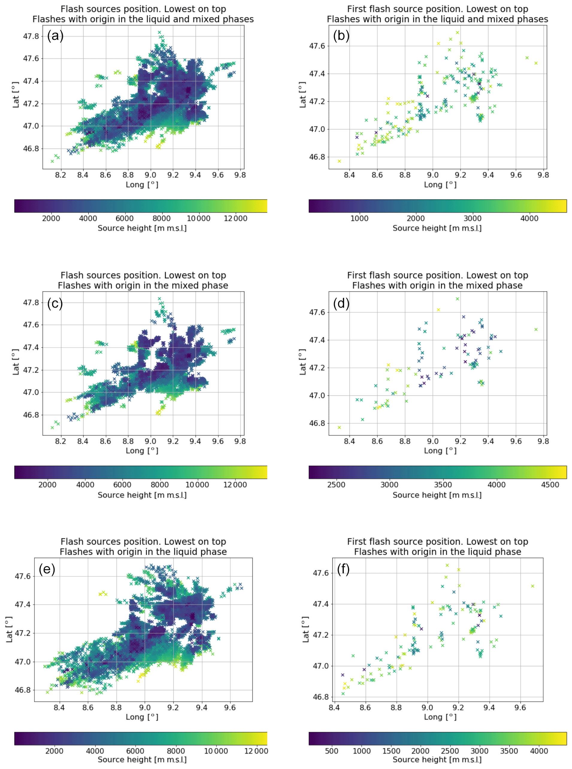
Figure 14Position of detected VHF sources for the days examined. (a, c, e) All VHF sources. (b, d, f) Only the first sources of each flash. From top to bottom: flashes with an origin in the liquid- and mixed-phase regions, flashes with an origin in the mixed-phase region, and flashes with an origin in the liquid-phase region.
Regarding the time of occurrence (see Fig. 15a), it is interesting to note that those types of flashes are distributed in a more uniform manner than when considering all the flashes. The flash duration distribution (Fig. 15b) shows that most flashes are relatively short-lived. The median duration of NSP flashes is 150 ms. They also cover a reduced area with a median of 50 km2 (see Fig. 15c).
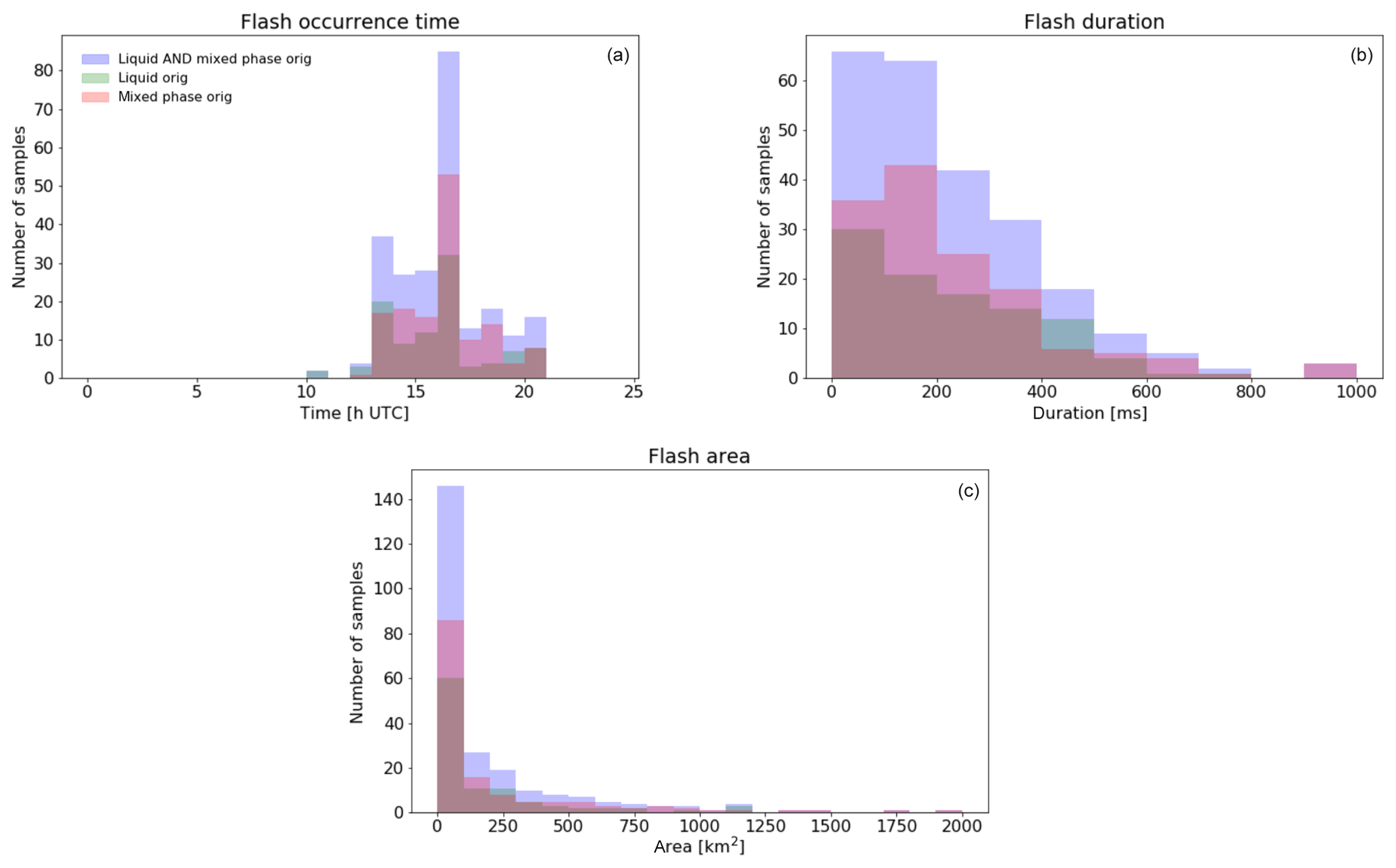
Figure 15Distribution of the flashes for all days analysed: (a) time of occurrence, (b) duration and (c) the 2-D projection area over the day for all days analysed. Bluish area: flashes with an origin in the liquid- and mixed-phase regions. Greenish area: flashes with an origin in the mixed-phase region. Reddish area: flashes with an origin in the liquid-phase region. Note that the values outside of the histogram range are added to the bins at the extremes.
In terms of source power (Fig. 16), when all VHF sources are considered, these flashes have a lower median than the general data, 18.5 dBm. When only the first VHF source in the flash is considered, the median power is 19.5 dBm for MP flashes and 18.5 dBm for LP flashes. It should be noticed that the distribution is not Gaussian-like but has two distinct peaks. A main one at roughly 20 dBm and a second one around 5 dBm, although this could simply be due to undersampling.
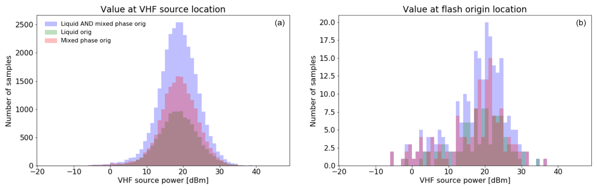
Figure 16Histogram of VHF sources power for all days analysed. (a) All sources. (b) Only the first sources of each flash. Bluish area: flashes with an origin in the liquid- and mixed-phase regions. Greenish area: flashes with an origin in the mixed-phase region. Reddish area: flashes with an origin in the liquid-phase region. Note that the values outside of the histogram range are added to the bins at the extremes.
Regarding the altitude of the VHF sources, there are remarkable differences with the global data (see Fig. 17a and b). As it should be expected NSP flashes are first detected at low altitudes (median of 3500 for MP flashes and 3200 for LP flashes), but their altitude when considering all sources has a bimodal distribution with a main peak at 3600 for MP flashes (3800 for LP flashes) and another roughly at 9000 for both. These data are further confirmed when looking at the temperature from the model (Fig. 17 bottom panels). When first detected, NSP flashes are located in regions with a temperature of 0∘C or a positive temperature, but they seem to extend higher up and concentrate in two main layers, one roughly at −5∘C and the other at −30∘C.
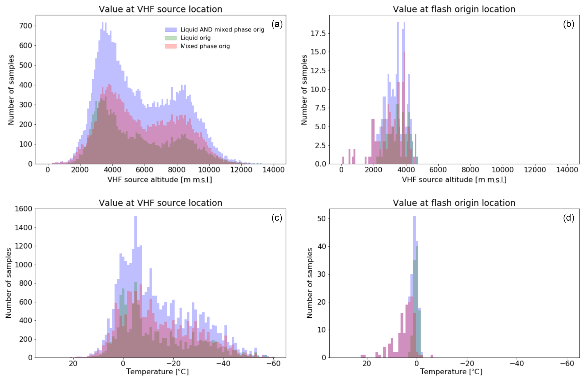
Figure 17Histogram during all days analysed of (a) VHF sources altitude, (b) only the first sources of each flash altitude, (c) all sources model air temperature, and (d) the first source's model air temperature. Bluish area: flashes with an origin in the liquid- and mixed-phase regions. Greenish area: flashes with an origin in the mixed-phase region. Reddish area: flashes with an origin in the liquid-phase region. Note that the values outside of the histogram range are added to the bins at the extremes.
The distribution of the polarimetric variables (see Fig. 18) has significant differences with the global data. The reflectivity has a uniform-like distribution extending from roughly 10 to 50 dBZ, with two barely visible peaks at 10 and 40 dBZ. There is not enough data to fully characterise the reflectivity at the flash origin, but it appears to have a Gaussian-like distribution with a median of 35.5 dBZ for NSP flashes and 32 and 40 dBZ when stratifying into MP and LP flashes, respectively. Zdr has a Gaussian-like shape centred at 0 dB when considering all VHF sources. When considering only the flash origin, the distribution is also Gaussian-like but with a positive median of 0.3 dB for NSP flashes (0.3 and 0.6 for MP and LP flashes, respectively). ρhv also has a much wider distribution than the global data, particularly when considering the flash origin. The mode is 0.997 for NSP (0.998 for MP flashes and 0.994 for LP flashes). Kdp is skewed towards positive values. The large prevalence of values 2 or larger in LP flashes is particularly remarkable.
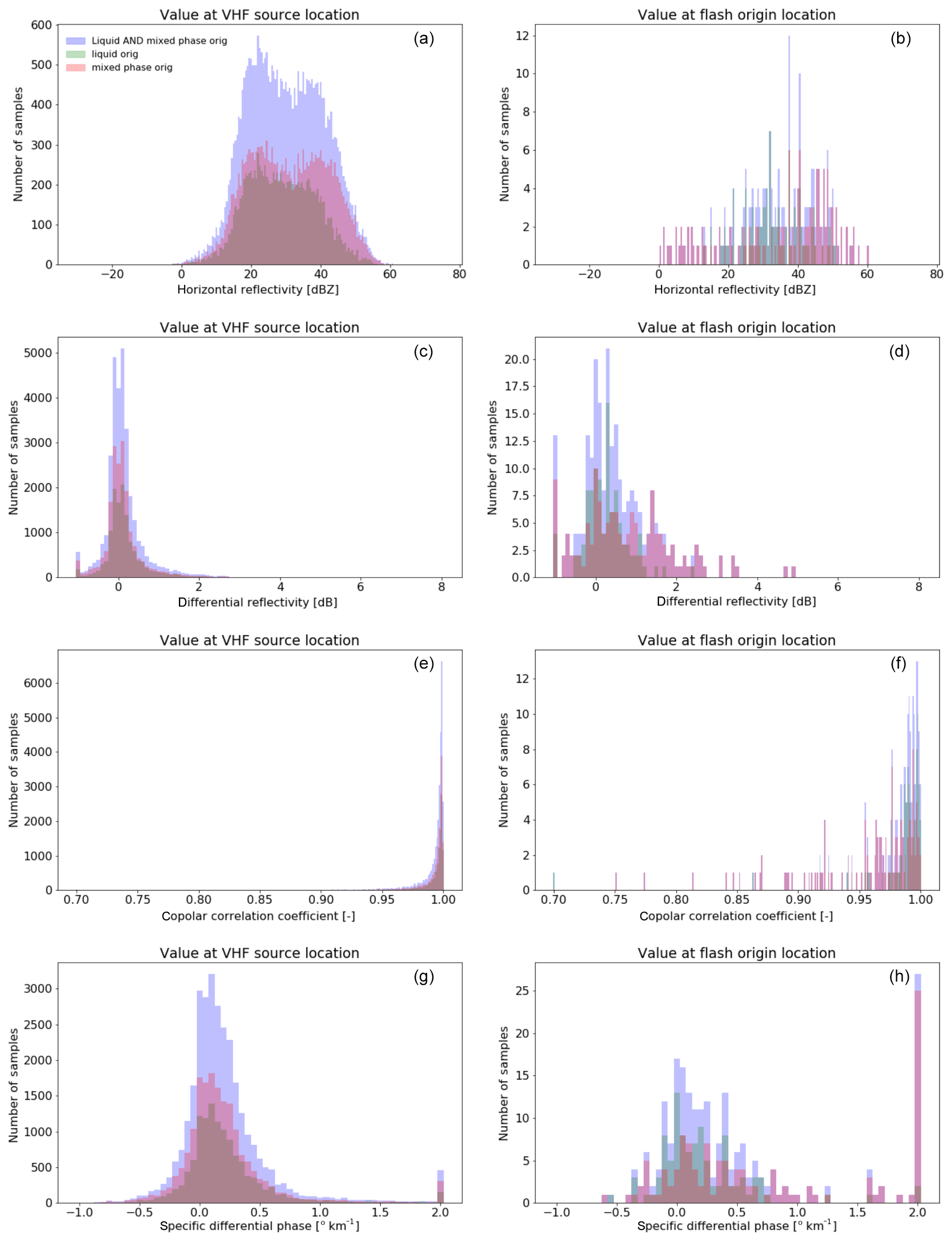
Figure 18Histogram during all days analysed of, from top to bottom, Zh, Zdr, ρhv and Kdp. (a, c, e, g) All sources. (b, d, f, h) The first source only. Bluish area: Flashes with an origin in the liquid- and mixed-phase regions. Greenish area: flashes with an origin in the mixed-phase region. Reddish area: flashes with an origin in the liquid-phase region. Note that the values outside of the histogram range are added to the bins at the extremes.
Figure 19a and Table 3 show the distribution of the dominant hydrometeors at the flash source locations. There are remarkable differences with respect to the global data. When considering NSP flashes, as usual the most common hydrometeor is rimed particles with 48.4 % but it is followed by dry snow with solid hail being the third most common. A large percentage of sources are located in areas of rain and wet snow. When further stratifying the data according to the flash origin, it can be seen that there is a larger proportion of sources located in the mixed phase for MP flashes with respect to LP flashes. The most salient feature is a significant increase in the solid hail proportion of LP flashes. What is most remarkable though is that when examining the entropy of the hydrometeor classification (see Fig. 19 middle panels) at the flash origin, it is much higher than that of the global data. Indeed, LP flashes have an entropy mode of 0.5 and MP flashes have an even higher entropy mode of 0.6. That translates into a higher proportion of flashes with an origin in radar gates containing a mix of at least two and up to five hydrometeors (see Fig. 19e and f).
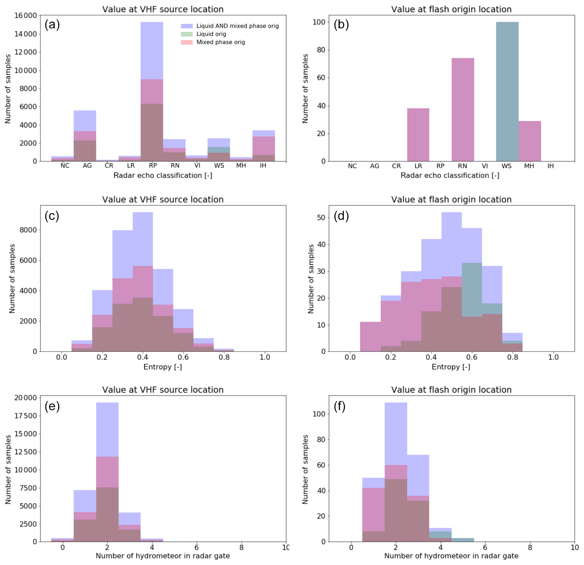
Figure 19Histogram during all days analysed of, from top to bottom, the dominant hydrometeor at the radar gate collocated with the VHF source position, the hydrometeor-classification-derived entropy at the radar gate collocated with the VHF source position, and the number of hydrometeor types with a significant presence at the radar gate collocated with the VHF source position. (a, c, e) All sources. (b, d, f) The first source only. Bluish area: flashes with an origin in the liquid- and mixed-phase regions. Greenish area: flashes with an origin in the mixed-phase region. Reddish area: flashes with an origin in the liquid-phase region. Note that the values outside of the histogram range are added to the bins at the extremes.
Figure 20 examines the most likely combination of hydrometeors at the location of the VHF sources. Unlike in the other data analysed, when all VHF sources are considered, the most common combination is that of rimed particles and snow, followed by rimed particles and dry hail. The most striking feature when looking at the flash origin is that the most-dominant combination is a mixture. In the case of MP flashes the most likely combination is wet snow and rain, followed by wet snow and rimed particles. LP flashes, on the other hand, have a mixture of rain and wet snow as the most likely.
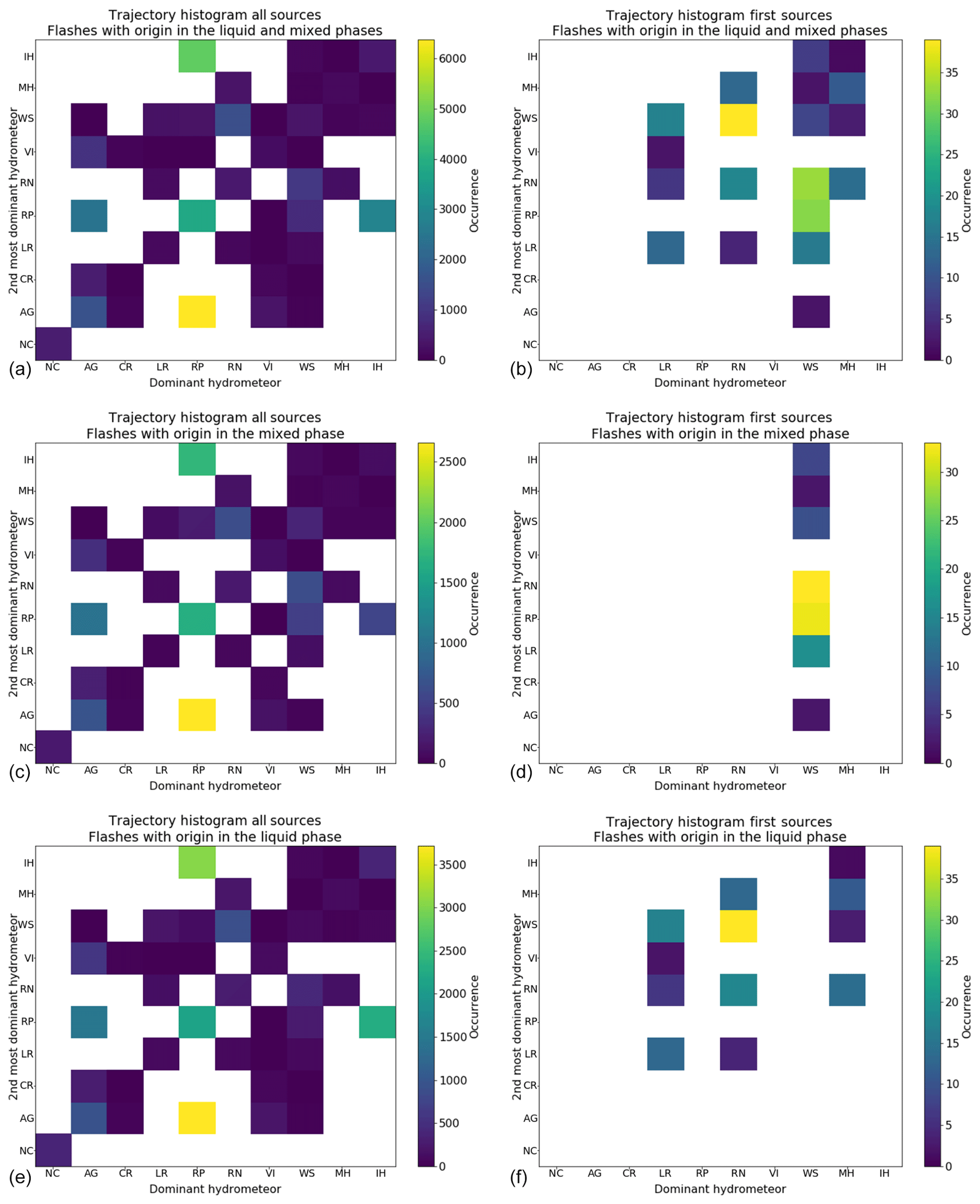
Figure 20A 2-D histogram of the type of the most-dominant and second most-dominant hydrometeor at the radar gate, collocated with the VHF source position. From top to bottom: Flashes with an origin in the liquid- and mixed-phase regions, flashes with an origin in the mixed-phase region, and flashes with an origin in the liquid-phase region. (a, c, e) All VHF sources in the flash. (b, d, f) Only the first VHF sources.
3.6 Discussion
Our dataset is dominated by data taken from 2 days: 1 August and 19 July. Both of these days represent 62% of the total number of flashes in the dataset but 86 % of the CG flashes and an outstanding 93 % of the CG+ flashes, a fact that has to be taken into account in order to interpret the results.
Most of the lightning activity during the 8 d analysed took place in the late afternoon. This seems to hint that a strong diurnal cycle, possibly reinforced by topographically induced wind systems, is what enables the level of convection necessary to trigger the lightning production mechanism (Trefalt et al., 2018). The passage of a cold front, typically from west-southwest to east-northeast in this region and synchronised with the diurnal cycle, might have increased the severity of the storms and had a positive impact on lightning production (Schemm et al., 2016). Observing the synoptic situation on the days analysed (not shown) this seems to be the case for the 1 August and the 10 and 30 July.
Most flashes were intra-cloud and only 9 % reached the ground, although this percentage varied widely from day to day, from a minimum of 1.5 % on 1 August to 17.6 % on 29 June. This result is consistent with that reported for storms during the summer period in the Ebro Valley (6.9 %) by López et al. (2017), which is the largest study with LMA data in the Mediterranean basin so far. Also consistent with that study, IC flashes tended to be shorter lived and of a smaller area than CG flashes. Flashes with an origin in the liquid- or mixed-phase layers of precipitation represented approximately 2 % of the dataset. Here there were again large day-to-day variations, from 1.1 % to 12.4 %.
The large majority of the flashes detected in our study originated in areas where rimed particles and/or solid hail were dominant. In a significant number of cases, the presence of other hydrometeors such as aggregates was non-negligible. Most flashes had an origin at relatively high altitudes (8000–9000 ). It is interesting to notice that, examining the median origin altitude of individual days (not shown) it can be observed that on days with less activity, the flash origin altitude is remarkably lower (4000–5000 ). Although no data were available during the campaign about the vertical wind at the onset of lightning, the widespread presence of rimed particles makes it very likely that, either at the onset of lightning or moments before, a significant number of super-cooled liquid water was present. Considering the altitude at which they were located, it is also safe to assume that flashes were most likely originated in transition areas between regions dominated by rimed particles and regions where the effects of the updraft were diminished and ice crystals or aggregates were dominant. Overall the data agrees with the graupel–ice collision mechanism (e.g. Takahashi, 1978; Brooks and Saunders, 1994), whereby individual particles acquire charge by collisions between precipitation particles and cloud particles, and gravity acts as a charge separator by pulling down most of the precipitating particles (i.e. rimed particles), while cloud particles (i.e. ice crystals or small aggregates) remain aloft. A shallower region dominated by rimed particles seems to result in lower lightning activity. Thus, in line with research from past studies (e.g. Petersen and Rutledge, 1998; Wiens et al., 2005), we find a relationship between the vertical extent of the regions dominated by rimed particles and the intensity of lightning activity.
When analysing GC flashes in detail we found that, with respect to IC flashes, there was a remarkable increase in flashes with an origin in regions dominated by hail and a noticeable increase in those with an origin in the liquid- and mixed-phase regions. That, coupled with a lower median origin altitude, suggests that flashes generated at the lower parts of the convective system are more likely to reach the ground. The general picture that emerges from these considerations is that of a classical tripole (Williams, 1989) with a small positively charged layer at the bottom (close or at the melting layer), a higher negative layer at the centre (in a region of high density of rimed particles) and a positive layer at the top (in the region where fewer rimed particles are formed and more ice crystals and aggregates are present). Most of the flashes are generated in the transition between the top negative and positive layers and propagate through the negative layer. The bottom layer tends to be less active but flashes generated there are more likely to reach the ground.
Our dataset contained an unusually high proportion of +CG flashes with respect to −CG flashes. That is mostly due to the very large proportion of +CG flashes in 3 out of the 8 d analysed. On those days hail was reported, and hence those results confirm past observations that associate and increase in +CG flashes with hail on the ground (e.g. Pineda et al., 2016; Kouketsu et al., 2017). The origins and the paths of the +CG flashes emerging from our data are not clear-cut. It is somehow surprising that the percentage of flashes that have an origins in regions where hail is dominant is lower than that of −CG flashes. It is also interesting to notice that there is simultaneously an increase in the percentage of flashes with origins in regions where aggregates are dominant (i.e. high up in the cloud structure) and an increase in flashes having origins in the mixed-phase and liquid-phase layers. Coupling that with a more uniform distribution of the altitude of the flash origin and the reflectivity values it emerges that +CG flashes have multiple generating mechanisms with none of them being dominant.
In regular storms, they may be generated at the transition between the lower positive layer and the negative layer of the classical tripole structure (which would result in a significant percentage being generated in areas of melting hail and wet snow) or they may be generated at the top positive layer (and thus a significant percentage would have an origin in aggregate areas). That is the likely scenario for those days where the percentage of +CG flashes with respect to the total is in line with what has been reported in past literature. However, most flashes present in the statistics were generated on two particular days. For those days we suspect that a significant percentage of flashes have been generated at the transition between the top positive and negative layers in an inverted tripole structure (Bruning et al., 2014). That would explain both the lower percentage of hail as the most-dominant hydrometeor in the statistics (since at those altitudes likely smaller rimed particles may be dominant) and the high altitude at which those flashes tend to originate.
The triggering mechanisms for flashes first detected in the liquid- or mixed-phase layers of a storm seem to be significantly different than those of the other lightning types. Examining the lightning path shows that they are much less likely to propagate through areas where hail is dominant. In contrast, they are significantly more likely to propagate in areas of dry snow. Therefore, it seems that they are less likely to be generated in areas of deep convection. In fact the lowest percentage of this type of lightning is registered on the 2 days with the most lightning activity. The behaviour of these flashes seems to be in good agreement with upward lightning, probably triggered by other lightning in the area. In the first place they are highly concentrated in the mountainous areas with a clear hot spot at the actual Säntis tower. In line with the studies performed specifically over the Säntis tower during the campaign (Pineda et al., 2019), a vast majority of flashes propagate upwards, up to areas of transition between rimed particles and dry snow and then extend horizontally within those areas.
We have presented an analysis of a large dataset of lightning and polarimetric weather radar data collected in the context of a lightning measurement campaign that took place in the summer of 2017 in the area surrounding Säntis, in northeastern Switzerland. In this campaign, for the first time in the Alps, a lightning mapping array was deployed. This paper focuses on data from 8 d where lightning activity was registered in the immediate vicinity of the Säntis tower. A total of 1 586 394 VHF sources, corresponding to 12 062 flashes (i.e. and average of 132 sources per flash) were detected by the LMA.
In this paper we have investigated the characteristics of the LMA flashes and related their VHF sources to co-located polarimetric radar measurements in order to determine the characteristics of the precipitation systems that enable the initiation and propagation of lightning. We have performed a general assessment and proceeded to stratify the data into the usual categories, i.e. intra-cloud, cloud-to-ground (positive or negative according to the associated EUCLID strokes) and flashes with an origin in the liquid- and mixed-phase layers as a proxy for upward lightning.
The general data analysis shows that there is a clear diurnal cycle in the days analysed with most flashes occurring in the late afternoon. Most lightning-producing systems travelled from southwest to northeast, roughly following the foothills of the Alps. VHF sources are more likely to be detected at altitudes between 3000 and 9000 . Their origin is more likely to be located at altitudes between 7000 to 9000 . Flashes thus originate in the upper part of convective clouds and either propagate at roughly the same altitude or move towards a lower layer. Most of the flashes originate in areas of high reflectivity (roughly 40 dBZ), low Zdr, low Kdp and high ρhv. A large majority of flashes originate in regions with a high concentration of particles with a certain degree of riming (either small rimed particles or solid hail), and, for the most part, they propagate within such regions. However, these regions are characterized by a high entropy and the radar resolution volume is likely to contain more than one hydrometeor type in significant proportions. The most likely combination of hydrometeors is rimed particles and solid hail, regardless of which one is dominant. Very few flashes originate in the mixed phase or liquid phase of precipitation and the number of VHF sources in those regions is also rather small, suggesting that flashes may transit through them but with a vertical direction.
Most of the examined flashes did not produce an associated EUCLID CG stroke, i.e. they were IC. CG flashes constitute approximately 10 % of the total dataset. There are significant differences between IC and CG flashes. CG flashes tend to generate more VHF sources, last significantly longer and have a larger projected area. The median altitude at which they are generated is lower than the IC ones and the temperature in the regions of generation is higher, a clear indicator that they are generated lower in the cloud. The co-located polarimetric variables have fairly similar distributions to those of the IC flashes, except that generally speaking they are wider. The reflectivity at the flash origin location, in particular, has a significantly larger median, suggesting that CG flashes are more likely to occur in regions of higher particle concentration and/or larger particle size and density, increased, for example, as a consequence of riming. That aspect is further confirmed by an increased proportion of flashes having their origin in areas where solid hail is the dominant hydrometeor. Indeed, the most likely combination of hydrometeors at the CG flash origin is one having solid hail as the most dominant and rimed particles as the second most dominant.
We have also attempted to further stratify the LMA flashes associated with EUCLID CG strokes into those generating a positive stroke and those generating a negative stroke. Roughly two-thirds of the flashes in the dataset are −CG and one-third are +CG. The characteristics of both types of flashes are rather similar although with some significant differences. +CG flashes tend to cover a larger area. −CG flashes are more likely to be associated with multiple EUCLID strokes. The median of the signal power at the origin of the discharge is slightly larger for +CG flashes. The altitude and temperature distributions also have significant differences. +CG flashes originate at a significantly lower altitude than −CG flashes. When all VHF sources are considered, the distribution of −CG flashes is bimodal while the distribution of +CG flashes is Gaussian-like. This would suggest that −CG flashes tend to propagate in multiple layers while +CG flashes have a more vertical structure. There are not many differences between the distribution of polarimetric variables of −CG and +CG flashes. The most remarkable difference is in the distribution of the reflectivity when all VHF sources are considered. −CG flashes have a Gaussian-like shape while +CG flashes have an almost uniform distribution. Again, this would suggest that −CG flashes are more likely to propagate in the cloud layer where they originated. whereas +CG flashes have a more vertical structure. As with all the data analysed, the entropy of the hydrometeor classification is rather high and it is very likely to have multiple hydrometeor types with significant proportions within a radar resolution volume. The proportion of dominant hydrometeors is similar for both types of flashes. The main difference is a larger percentage of −CG flashes that have an origin in areas of solid hail. However, in both cases the most likely combination of hydrometeors at the flash origin is solid hail and rimed particles, albeit in different proportions.
We have also examined the characteristics of LMA flashes that have their origin in the liquid- and mixed-phase layers. The rationale for that is that there is an increased likelihood that those flashes are upward lightning. Only 241 flashes in the dataset had an origin in the mixed-phase or liquid-phase layers and, of those, 141 had an origin in the liquid layer. One aspect that sets apart this type of flash is that their origins are not randomly distributed within the path of the storm but we have identified areas of higher concentration. One of them is the Säntis tower and another is the Gamsberg. That is a strong indicator that indeed these flashes originate by interactions with the terrain and man-made objects. These flashes tend to be short-lived and occupy a reduced projected area, which would indicate a vertical orientation. As would be expected, they are first detected at low altitudes but their altitude distribution is bimodal with a secondary peak at roughly 9000 , a rather high altitude within the precipitating system. The distribution of the polarimetric variables is also fairly different from the rest of the data analysed. Overall, these distributions suggest that this sort of flash encounters a larger variety of precipitation regimes along their path. This is further confirmed by the fact that the entropy of the hydrometeor classification is even higher than in the previously examined cases, particularly at the flash origin, and it is rather common to have more than two species in significant proportions at the flash origin. Unlike with the rest of the data examined, rimed particles or solid hail are not part of the most common species in the mixture at the location of the flash origin, the most common being a mixture of wet snow and rain. However, when examining all the VHF sources, the most common mixture at the VHF source position is rimed particles and snow. Solid hail, on the other hand, does not have as much of a significant presence as it does the global data. This would indicate that this sort of flashes can be initiated even in moderate convection conditions.
From our analysis we can conclude that a systematic detection of lightning with polarimetric radar data is not possible, but radar data can be extremely useful to indicate regions with favourable conditions for lightning initiation. A high concentration, i.e. high reflectivity, of rimed particles and/or solid hail and a high entropy of the hydrometeor classification are a primary indicator of lightning activity. Whether the generated flashes are IC or CG is not something that can be readily determined by just observing the polarimetric radar data, although there are indicators that suggest that CG flashes tend to generate at a lower cloud level and, therefore, looking at the vertical structure of the precipitating system can provide hints on whether the flashes are more likely to be contained within the cloud or propagate to the ground. Upward lightning poses another challenge because this type of flash has not shown as clear radar signatures as the rest of the examined categories and seem to be driven mostly by the interaction of the storm with the terrain and man-made structures. Nevertheless, in that case a degree of convection also seems to be necessary to initiate a flash. In any case, to estimate the probability of this sort of flashes it seems clear that either the orography (including man-made structures) or a climatology has to be included in any flash nowcasting system.
Code used to post-process the radar data is available on github https://github.com/meteoswiss-mdr (last access: 21 May 2019). Data are available on request by contacting the authors.
JFiV performed the radar data processing and the data analysis contained in this paper. NB and JG contributed to the radar data processing and data interpretation. OvdV, DR, JM, NP, AS, AM, MA, MR and FRH deployed the LMA network and processed its data. UG and AH advised on the content of the paper. JFiV prepared the paper with contributions from all authors.
The authors declare that they have no conflict of interest.
This research has been supported by the Swiss National Science Foundation (grant no. 200020_175594), the Horizon 2020 Framework Programme (grant LLR 737033), the Spanish Ministry of Economy, and the European Regional Development Fund (FEDER) (grant nos. ESP2013-48032-C5-3-R, ESP2015-69909-C5-5-R and ESP2017-86263-C4-2-R.)
This paper was edited by Gianfranco Vulpiani and reviewed by three anonymous referees.
Azadifar, M.: Characteristics of Upward Lightning Flashes, PhD thesis, Swiss Federal Institute of Technology, 2017. a
Azadifar, M., Rachidi, F., Rubinstein, M., Paolone, M., Diendorfer, G., Pichler, H., Schulz, W., Pavanello, D., and Romero, C.: Evaluation of the performance characteristics of the European Lightning Detection Network EUCLID in the Alps region for upward negative flashes using direct measurements at the instrumented Säntis Tower, J. Geophys. Res.-Atmos., 121, 595–606, https://doi.org/10.1002/2015JD024259, 2015. a, b, c
Besic, N., Figueras i Ventura, J., Grazioli, J., Gabella, M., Germann, U., and Berne, A.: Hydrometeor classification through statistical clustering of polarimetric radar measurements: a semi-supervised approach, Atmos. Meas. Tech., 9, 4425–4445, https://doi.org/10.5194/amt-9-4425-2016, 2016. a
Besic, N., Gehring, J., Praz, C., Figueras i Ventura, J., Grazioli, J., Gabella, M., Germann, U., and Berne, A.: Unraveling hydrometeor mixtures in polarimetric radar measurements, Atmos. Meas. Tech., 11, 4847–4866, https://doi.org/10.5194/amt-11-4847-2018, 2018. a, b
Brooks, I. M. and Saunders, C.: An experimental investigation of the inductive mechanism of thunderstorm electrification, J. Geophys. Res.-Atmos., 99, 10627–10632, https://doi.org/10.1029/93JD01574, 1994. a
Bruning, E. C., Rust, W. D., Schuur, T. J., MacGorman, D. R., Krehbiel, P. R., and Rison, W.: Electrical and Polarimetric Radar Observations of a Multicell Storm in TELEX, Mon. Weather Rev., 135, 2525–2544, https://doi.org/10.1175/MWR3421.1, 2007. a
Bruning, E. C., Weiss, S. A., and Calhoun, K. M.: Continuous variability in thunderstorm primary electrification and an evaluation of inverted-polarity terminology, Atmos. Res., 135–136, 274–284, https://doi.org/10.1016/j.atmosres.2012.10.009, 2014. a
Calhoun, K. M., MacGorman, D. R., Ziegler, C. L., and Biggerstaff, M. I.: Evolution of Lightning Activity and Storm Charge Relative to Dual-Doppler Analysis of a High-Precipitation Supercell Storm, Mon. Weather Rev., 141, 2199–2223, https://doi.org/10.1175/MWR-D-12-00258.1, 2013. a
Chronis, T., Lang, T., Koshak, W., Blakeslee, R., Christian, H., McCaul, E., and Bailey, J.: Diurnal characteristics of lightning flashes detected over the Sao Paulo lightning mapping array, J. Geophys. Res.-Atmos., 120, 11799–11808, https://doi.org/10.1002/2015JD023960, 2015. a
Defer, E., Pinty, J.-P., Coquillat, S., Martin, J.-M., Prieur, S., Soula, S., Richard, E., Rison, W., Krehbiel, P., Thomas, R., Rodeheffer, D., Vergeiner, C., Malaterre, F., Pedeboy, S., Schulz, W., Farges, T., Gallin, L.-J., Ortéga, P., Ribaud, J.-F., Anderson, G., Betz, H.-D., Meneux, B., Kotroni, V., Lagouvardos, K., Roos, S., Ducrocq, V., Roussot, O., Labatut, L., and Molinié, G.: An overview of the lightning and atmospheric electricity observations collected in southern France during the HYdrological cycle in Mediterranean EXperiment (HyMeX), Special Observation Period 1, Atmos. Meas. Tech., 8, 649–669, https://doi.org/10.5194/amt-8-649-2015, 2015. a
Diendorfer, G., Pichler, H., and Mair, M.: Some Parameters of Negative Upward-Initiated Lightning to the Gaisberg Tower (2000–2007), IEEE T. Electromagn. C., 51, 443–452, https://doi.org/10.1109/TEMC.2009.2021616, 2009. a
Doviak, R. and Zrnic, D.: Doppler Radar and Weather Observations, Dover Books on Engineering Series, Dover Publications, Dover Publications, Inc., 31 East 2nd Street, Mineola, N.Y. 11501, available at: https://books.google.ch/books?id=ispLkPX9n2UC (last access: 21 May 2019), 2006. a
Figueras i Ventura, J., Honoré, F., and Tabary, P.: X-Band Polarimetric Weather Radar Observations of a Hailstorm, J. Atmos. Ocean. Tech., 30, 2143–2151, https://doi.org/10.1175/JTECH-D-12-00243.1, 2013. a
Figueras i Ventura, J., Leuenberger, A., Kuensch, Z., Grazioli, J., and Germann, U.: Pyrad: A Real-Time Weather Radar Data Processing Framework Based on Py-ART, in: 38th AMS Conference on Radar Meteorology, Chicago, IL, USA, 2017. a
Fuchs, B. R., Rutledge, S. A., Bruning, E. C., Pierce, J. R., Kodros, J. K., Lang, T. J., MacGorman, D. R., Krehbiel, P. R., and Rison, W.: Environmental controls on storm intensity and charge structure in multiple regions of the continental United States, J. Geophys. Res.-Atmos., 120, 6575–6596, https://doi.org/10.1002/2015JD023271, 2015. a, b
Fuchs, B. R., Bruning, E. C., Rutledge, S. A., Carey, L. D., Krehbiel, P. R., and Rison, W.: Climatological analyses of LMA data with an open-source lightning flash-clustering algorithm, J. Geophys. Res.-Atmos., 121, 8625–8648, https://doi.org/10.1002/2015JD024663, 2016. a
Germann, U., Boscacci, M., Gabella, M., and Sartori, M.: Peak performance: Radar design for prediction in the Swiss Alps, Meteorological Technology International, 4, 42–45, 2015. a
Gourley, J. J., Tabary, P., and Parent du Chatelet, J.: Data Quality of the Meteo-France C-Band Polarimetric Radar, J. Atmos. Ocean. Tech., 23, 1340–1356, https://doi.org/10.1175/JTECH1912.1, 2006. a
He, L., Azadifar, M., Rachidi, F., Rubinstein, M., Rakov, V. A., Cooray, V., Pavanello, D., and Xing, H.: An Analysis of Current and Electric Field Pulses Associated With Upward Negative Lightning Flashes Initiated from the Säntis Tower, J. Geophys. Res.-Atmos., 123, 4045–4059, https://doi.org/10.1029/2018JD028295, 2018. a
Hubbert, J. C., Ellis, S. M., Chang, W.-Y., Rutledge, S., and Dixon, M.: Modeling and Interpretation of S-Band Ice Crystal Depolarization Signatures from Data Obtained by Simultaneously Transmitting Horizontally and Vertically Polarized Fields, J. Appl. Meteorol. Clim., 53, 1659–1677, https://doi.org/10.1175/JAMC-D-13-0158.1, 2014. a
Koshak, W. J., Solakiewicz, R. J., Blakeslee, R. J., Goodman, S. J., Christian, H. J., Hall, J. M., Bailey, J. C., Krider, E. P., Bateman, M. G., Boccippio, D. J., Mach, D. M., McCaul, E. W., Stewart, M. F., Buechler, D. E., Petersen, W. A., and Cecil, D. J.: North Alabama Lightning Mapping Array (LMA): VHF Source Retrieval Algorithm and Error Analyses, J. Atmos. Ocean. Tech., 21, 543–558, https://doi.org/10.1175/1520-0426(2004)021<0543:NALMAL>2.0.CO;2, 2004. a
Kouketsu, T., Uyeda, H., Ohigashi, T., and Tsuboki, K.: Relationship between cloud-to-ground lightning polarity and the space-time distribution of solid hydrometeors in isolated summer thunderclouds observed by X-band polarimetric radar, J. Geophys. Res.-Atmos., 122, 8781–8800, https://doi.org/10.1002/2016JD026283, 2017. a
Kumjian, M. R. and Deierling, W.: Analysis of Thundersnow Storms over Northern Colorado, Weather Forecast., 30, 1469–1490, https://doi.org/10.1175/WAF-D-15-0007.1, 2015. a
Lang, T. J., Miller, L. J., Weisman, M., Rutledge, S. A., Barker, L. J., Bringi, V. N., Chandrasekar, V., Detwiler, A., Doesken, N., Helsdon, J., Knight, C., Krehbiel, P., Lyons, W. A., MacGorman, D., Rasmussen, E., Rison, W., Rust, W. D., and Thomas, R. J.: The Severe Thunderstorm Electrification and Precipitation Study, B. Am. Meteorol. Soc., 85, 1107–1126, https://doi.org/10.1175/BAMS-85-8-1107, 2004. a
López, J. A., Pineda, N., Montanyà, J., van der Velde, O., Fabró, F., and Romero, D.: Spatio-temporal dimension of lightning flashes based on three-dimensional Lightning Mapping Array, Atmos. Res., 197, 255–264, https://doi.org/10.1016/j.atmosres.2017.06.030, 2017. a, b
Lund, N. R., MacGorman, D. R., Schuur, T. J., Biggerstaff, M. I., and Rust, W. D.: Relationships between Lightning Location and Polarimetric Radar Signatures in a Small Mesoscale Convective System, Mon. Weather Rev., 137, 4151–4170, https://doi.org/10.1175/2009MWR2860.1, 2009. a
MacGorman, D. R., Rust, W. D., Schuur, T. J., Biggerstaff, M. I., Straka, J. M., Ziegler, C. L., Mansell, E. R., Bruning, E. C., Kuhlman, K. M., Lund, N. R., Biermann, N. S., Payne, C., Carey, L. D., Krehbiel, P. R., Rison, W., Eack, K. B., and Beasley, W. H.: TELEX The Thunderstorm Electrification and Lightning Experiment, B. Am. Meteorol. Soc., 89, 997–1014, https://doi.org/10.1175/2007BAMS2352.1, 2008. a
Mattos, E. V., Machado, L. A. T., Williams, E. R., and Albrecht, R. I.: Polarimetric radar characteristics of storms with and without lightning activity, J. Geophys. Res.-Atmos., 121, 14201–14220, https://doi.org/10.1002/2016JD025142, 2016. a
Mostajabi, A., Pineda, N., Sunjerga, A., Romero, D., Azadifar, M., van der Velde, O., Montanyà, J., Diendorfer, G., Rubinstein, M., and Rachidi, F.: LMA Campaign for the Observation of Upward Lightning at the Santis Tower During Summer 2017: Preliminary Results, in: XVI International Conference on Atmospheric Electricity, Nara, Japan, 2018. a
Payne, C. D., Schuur, T. J., MacGorman, D. R., Biggerstaff, M. I., Kuhlman, K. M., and Rust, W. D.: Polarimetric and Electrical Characteristics of a Lightning Ring in a Supercell Storm, Mon. Weather Rev., 138, 2405–2425, https://doi.org/10.1175/2009MWR3210.1, 2010. a
Petersen, W. A. and Rutledge, S. A.: On the relationship between cloud-to-ground lightning and convective rainfall, J. Geophys. Res.-Atmos., 103, 14025–14040, https://doi.org/10.1029/97JD02064, 1998. a
Pineda, N., Rigo, T., Montanyà, J., and van der Velde, O. A.: Charge structure analysis of a severe hailstorm with predominantly positive cloud-to-ground lightning, Atmos. Res., 178–179, 31–44, https://doi.org/10.1016/j.atmosres.2016.03.010, 2016. a, b
Pineda, N., Figueras i Ventura, J., Romero, D., Mostajabi, A., Azadifar, M., Sunjerga, A., Rachidi, F., Rubinstein, M., Montanyà, J., van der Velde, O., Altube, P., Besic, N., Grazioli, J., Germann, U., and Williams, E. R.: Meteorological aspects of self-initiated upward ligthning at the Säntis tower (Switzerland), J. Geophys. Res.-Atmos., submitted, 2019. a
Proctor, D. E.: A hyperbolic system for obtaining VHF radio pictures of lightning, J. Geophys. Res., 76, 1478–1489, https://doi.org/10.1029/JC076i006p01478, 1971. a
Proctor, D. E.: VHF radio pictures of cloud flashes, J. Geophys. Res.-Oceans, 86, 4041–4071, https://doi.org/10.1029/JC086iC05p04041, 1981. a
Proctor, D. E., Uytenbogaardt, R., and Meredith, B. M.: VHF radio pictures of lightning flashes to ground, J. Geophys. Res.-Atmos., 93, 12683–12727, https://doi.org/10.1029/JD093iD10p12683, 1988. a
Rachidi, F., Rubinstein, M., Montanya, J., Bermudez, J., Sola, R. R., Sola, G., and Korovkin, N.: A Review of Current Issues in Lightning Protection of New-Generation Wind-Turbine Blades, IEEE T. Ind. Electron., 55, 2489–2496, https://doi.org/10.1109/TIE.2007.896443, 2008. a
Ribaud, J.-F., Bousquet, O., and Coquillat, S.: Relationships between total lightning activity, microphysics and kinematics during the 24 September 2012 HyMeX bow-echo system, Q. J. Roy. Meteor. Soc., 142, 298–309, https://doi.org/10.1002/qj.2756, 2016. a
Rison, W., Thomas, R. J., Krehbiel, P. R., Hamlin, T., and Harlin, J.: A GPS-based three-dimensional lightning mapping system: Initial observations in central New Mexico, Geophys. Res. Lett., 26, 3573–3576, https://doi.org/10.1029/1999GL010856, 1999. a
Romero, C., Paolone, M., Rubinstein, M., Rachidi, F., Rubinstein, A., Diendorfer, G., Schulz, W., Daout, B., Kälin, A., and Zweiacker, P.: A system for the measurements of lightning currents at the Säntis Tower, Electr. Pow. Syst. Res., 82, 34–43, https://doi.org/10.1016/j.epsr.2011.08.011, 2012. a
Romero, C., Rachidi, F., Rubinstein, M., Paolone, M., Rakov, V. A., and Pavanello, D.: Positive lightning flashes recorded on the Säntis tower from May 2010 to January 2012, J. Geophys. Res.-Atmos., 118, 12879–12892, https://doi.org/10.1002/2013JD020242, 2013. a
Ryzhkov, A., Diederich, M., Zhang, P., and Simmer, C.: Potential utilization of specific attenuation for rainfall estimation, mitigation of partial beam blockage, and radar networking, J. Atmos. Ocean. Tech., 31, 599–619, 2014. a
Saunders, C. P. R., Bax-norman, H., Emersic, C., Avila, E. E., and Castellano, N. E.: Laboratory studies of the effect of cloud conditions on graupel/crystal charge transfer in thunderstorm electrification, Q. J. Roy. Meteor. Soc., 132, 2653–2673, https://doi.org/10.1256/qj.05.218, 2006. a
Schemm, S., Nisi, L., Martinov, A., Leuenberger, D., and Martius, O.: On the link between cold fronts and hail in Switzerland, Atmos. Sci. Lett., 17, 315–325, https://doi.org/10.1002/asl.660, 2016. a
Schultz, C. J., Lang, T. J., Bruning, E. C., Calhoun, K. M., Harkema, S., and Curtis, N.: Characteristics of Lightning Within Electrified Snowfall Events Using Lightning Mapping Arrays, J. Geophys. Res.-Atmos., 123, 2347–2367, https://doi.org/10.1002/2017JD027821, 2018. a
Schulz, W., Diendorfer, G., Pedeboy, S., and Poelman, D. R.: The European lightning location system EUCLID – Part 1: Performance analysis and validation, Nat. Hazards Earth Syst. Sci., 16, 595–605, https://doi.org/10.5194/nhess-16-595-2016, 2016. a
Smorgonskiy, A., Rachidi, F., Rubinstein, M., Diendorfer, G., and Schulz, W.: On the proportion of upward flashes to lightning research towers, Atmos. Res., 129–130, 110–116, https://doi.org/10.1016/j.atmosres.2012.08.014, 2013. a
Snyder, J. C., Ryzhkov, A. V., Kumjian, M. R., Khain, A. P., and Picca, J.: A ZDR Column Detection Algorithm to Examine Convective Storm Updrafts, Weather Forecast., 30, 1819–1844, https://doi.org/10.1175/WAF-D-15-0068.1, 2015. a
Takahashi, T.: Riming Electrification as a Charge Generation Mechanism in Thunderstorms, J. Atmos. Sci., 35, 1536–1548, https://doi.org/10.1175/1520-0469(1978)035<1536:REAACG>2.0.CO;2, 1978. a
Tessendorf, S. A., Rutledge, S. A., and Wiens, K. C.: Radar and Lightning Observations of Normal and Inverted Polarity Multicellular Storms from STEPS, Mon. Weather Rev., 135, 3682–3706, https://doi.org/10.1175/2007MWR1954.1, 2007. a
Testud, J., Le Bouar, E., Obligis, E., and Ali-Mehenni, M.: The Rain Profiling Algorithm Applied to Polarimetric Weather Radar, J. Atmos. Ocean. Tech., 17, 332–356, https://doi.org/10.1175/1520-0426(2000)017<0332:TRPAAT>2.0.CO;2, 2000. a
Thomas, R. J., Krehbiel, P. R., Rison, W., Hunyady, S. J., Winn, W. P., Hamlin, T., and Harlin, J.: Accuracy of the Lightning Mapping Array, J. Geophys. Res.-Atmos., 109, https://doi.org/10.1029/2004JD004549, 2004. a
Trefalt, S., Martynov, A., Barras, H., Besic, N., Hering, A. M., Lenggenhager, S., Noti, P., Röthlisberger, M., Schemm, S., Germann, U., and Martius, O.: A severe hail storm in complex topography in Switzerland – Observations and processes, Atmos. Res., 209, 76–94, https://doi.org/10.1016/j.atmosres.2018.03.007, 2018. a
van der Velde, O. A. and Montanyà, J.: Asymmetries in bidirectional leader development of lightning flashes, J. Geophys. Res.-Atmos., 118, 13504–13519, https://doi.org/10.1002/2013JD020257, 2013. a, b
Vulpiani, G., Montopoli, M., Passeri, L. D., Gioia, A. G., Giordano, P., and Marzano, F. S.: On the Use of Dual-Polarized C-Band Radar for Operational Rainfall Retrieval in Mountainous Areas, J. Appl. Meteorol. Clim., 51, 405–425, https://doi.org/10.1175/JAMC-D-10-05024.1, 2012. a
Wiens, K. C., Rutledge, S. A., and Tessendorf, S. A.: The 29 June 2000 Supercell Observed during STEPS. Part II: Lightning and Charge Structure, J. Atmos. Sci., 62, 4151–4177, https://doi.org/10.1175/JAS3615.1, 2005. a
Williams, E. R.: The tripole structure of thunderstorms, J. Geophys. Res.-Atmos., 94, 13151–13167, https://doi.org/10.1029/JD094iD11p13151, 1989. a