Homogeneity criteria from AVHRR information within IASI pixels in a numerical weather prediction context

This article focuses on the selection of satellite infrared IASI (Infrared Atmospheric Sounding Interferometer) observations in the global numerical weather prediction (NWP) system ARPEGE (Action de Recherche Petite Echelle Grande Echelle). The observation simulation is performed with the sophisticated radiative transfer model RTTOV-CLD, which takes into account the cloud scattering and the multilayer clouds from atmospheric profiles and cloud microphysical profiles (liquid water content, ice content and cloud fraction).

The aim of this work is to select homogeneous scenes by using the information of the collocated Advanced Very High Resolution Radiometer (AVHRR) pixels inside each IASI field of view and to retain the most favourable cases for the assimilation of IASI infrared radiances. Two methods to select homogeneous scenes using homogeneity criteria already proposed in the literature were adapted: the criteria derived from Martinet et al. (2013) for cloudy sky selection in the French mesoscale model AROME (Applications of Research to Operations at MEsoscale) and the criteria from Eresmaa (2014) for clear-sky selection in the global model IFS (Integrated Forecasting System). A comparison between these methods reveals considerable differences, in both the method to compute the criteria and the statistical results. From this comparison a revised method representing a kind of compromise between the different tested methods is proposed and it uses the two infrared AVHRR channels to define the homogeneity criteria in the brightness temperature space. This revised method has a positive impact on the observation minus the simulation statistics, while retaining 36 % of observations for the assimilation. It was then tested in the NWP system ARPEGE for the clear-sky assimilation. These criteria were added to the current data selection based on the McNally and Watts (2003) cloud detection scheme. It appears that the impact on analyses and forecasts is rather neutral.

1 Introduction

Satellite observations are currently the dominant source of information for numerical weather prediction (NWP) systems. Their assimilation together with in situ observations give the atmosphere analysis, which is a necessary step in the definition of the initial conditions of the forecast. This analysis consists in finding the state of the atmosphere that is compatible with the different sources of observations, the dynamics of the atmosphere and a previous state of the model. In the Météo-France global model ARPEGE (Action de Recherche Petite Echelle Grande Echelle, Courtier et al., 1991), 70 % of used observations come from infrared hyperspectral sounders, of which IASI (Infrared Atmospheric Sounding Interferometer; Cayla, 2001) fills a large part. This sounder provides information about the atmospheric temperature and humidity, and through its window channels information about the land surface parameters in clear-sky and cloudy parameters can be obtained. However, the wealth of information provided by this type of sensor with its large number of channels or radiances (8461 per pixel in the case of IASI) and its overall coverage with a horizontal resolution of 12 km at nadir are far from being fully exploited. Indeed, the presence of clouds in the instrument field of view affects the majority of the observations and it prevents us from accurately simulating the radiances. In fact, NWP centres use only a small number of observations from these sounders mostly in the clear sky above clouds. Previous studies have shown that sensitive areas are often covered by clouds (McNally, 2002; Fourrié and Rabier, 2004) and different techniques have been developed in the frame of global models to use infrared radiances in these regions.

In the past, different approaches have been proposed for cloud detection. A method to detect clear channels from high-resolution infrared (IR) spectral instruments was proposed by McNally and Watts (2003) to assimilate channels unaffected by clouds.

At the Met Office, Pavelin et al. (2008) showed that it was possible to assimilate cloud-affected infrared radiances when retrieved cloud parameters are used as set constraints. The cloud-top pressure (CTOP) and the effective cloud fraction (Ne) are firstly retrieved by a one-dimensional variational data assimilation system (1D-Var) and then provided to four-dimensional variational data assimilation (4D-Var) for the assimilation of cloud-affected infrared radiances. The analysis is significantly improved over the first guess by this method and it is used operationally to assimilate cloud-affected hyperspectral infrared radiances. At ECMWF (European Centre for Medium-Range Weather Forecasts), McNally (2009) proposed a method based on two cloud parameters (CTOP and Ne) to directly assimilate cloud-affected IR radiances. In that case, the cloud parameters are determined with two channels. They are then introduced into the analysis control vector of the 4D-Var system of the global NWP model to constrain the minimization. At Météo-France, the cloud parameters (CTOP and Ne) are retrieved for AIRS and IASI cloud-affected radiances with the CO₂-slicing method (Menzel et al., 1983). Channels affected by clouds, for which the cloud-top pressure (CTOP) ranges from 650 to 900 hPa with an effective cloud fraction (Ne) of 1, are assimilated in addition to clear ones in the ARPEGE 4D-Var and the AROME (Applications of Research to Operations at MEsoscale) 3D-Var (Pangaud et al., 2009; Guidard et al., 2011).

As pointed out by Errico et al. (2007), studies on the assimilation of clouds and precipitation from satellite sensors started in the 1980s, and despite the encountered difficulties in implementing them, operational weather centres are now assimilating them with a clear benefit for the forecast quality. Efforts started with microwave radiances and direct all-sky microwave radiance assimilation is effective at ECMWF (Bauer et al., 2010) since 2009 and at NOAA (National Oceanic and Atmospheric Administration) NCEP (National Centers for Environmental Prediction) since 2016. Even though ECMWF focussed on the assimilation of microwave imaging and humidity-sounding channels and conversely, NOAA NCEP focussed on temperature channels from the Advanced Microwave Sounding Unit-A (AMSU-A), both centres noticed benefits of such an all-sky assimilation for the forecast quality (Geer et al., 2017; Zhu et al., 2016).

Concerning infrared radiance all-sky assimilation, no operational centre has yet assimilated infrared observations, but research has still started in this area. Many aspects have already been studied as the information on cloud microphysics brought by the adjoint sensitivity in the assimilation (Greenwald et al., 2002) or by the retrieval of cloudy infrared radiances (Martinet et al., 2013). In addition the sensitivity, the reproducibility and the nonlinearity of IR radiance simulations in the presence of multilayer clouds were studied using diagnosed cloud schemes (Chevallier et al., 2004; Stengel et al., 2010). These studies also showed beneficial results.

A step further was achieved with the study by Okamoto et al. (2014). They studied the assimilation of multilayer cloud-affected infrared radiances using the all-sky assimilation approach already implemented for microwave images at ECMWF. They particularly investigated the cloud effects on the differences between observations and simulations and thus proposed an appropriate quality check and dedicated observation errors.

In this study, we are interested in IASI observations, where the radiances are considered with collocated cluster statistical properties of the Advanced Very High Resolution Radiometer (AVHRR) also on board the Metop platform. AVHRR has a horizontal resolution of 1 km at nadir (Cayla, 2001). Collocated AVHRR data provide information on surface properties and the presence of clouds in the IASI field of view (FOV). They can therefore be used for cloud detection. The AVHRR cluster information associated with IASI has already proven to be useful for selection purposes in the context of cloudy data assimilation, with an explicit treatment of microphysical variables in the AROME model by Martinet et al. (2013). Eresmaa (2014) at ECMWF also used AVHRR cluster information for cloud detection and observation selection in the clear sky.

Martinet et al. (2013) selected cloudy scenes based on cloud homogeneity. This study was carried out in a 1D-Var framework using an advanced radiative transfer model (RTTOV-CLD) including profiles for liquid water content, ice water content and cloud fraction to simulate cloud-affected equivalents from background AROME fields. The persistence of cloud information brought by the analysis of cloud variables during a 3 h forecast was then evaluated successfully with a one-dimensional model AROME version (Martinet et al., 2014). Okamoto (2017) studied the impact of the super-observation homogeneity quality control on the Advanced Himawari Imager brightness temperature simulation. He concluded that for a larger size of super observations, the standard deviation threshold should be relaxed in order to keep sufficiently low brightness temperatures associated with high-level cloud because of the presence of more cloud heterogeneity in large size observations.

In this article, our objective is to determine homogeneity criteria valid for both clear and cloudy conditions, suitable for a NWP context using collocated AVHRR and IASI information. Section 2 describes the ARPEGE NWP system, the IASI instrument and the radiative transfer model RTTOV-CLD in cloudy sky conditions. In Sect. 3, information about the AVHRR clusters is detailed, the strengths and weaknesses of the different methods in selecting homogeneous observations are discussed, and the chosen method is presented together with a description of the selected observations. Section 4 depicts the impacts on analyses and forecasts of the assimilation of selected clear and cloudy IASI observations. Conclusion and perspectives are given in Sect. 5.

2 Experimental framework

2.1 The ARPEGE model and its 4D-Var system

The ARPEGE model is the global NWP model at Météo-France, used operationally since the early 1990s (Courtier et al., 1991). This system is fully integrated within the ARPEGE-IFS software conceived, developed and maintained in collaboration with ECMWF.

This spectral global model has a stretched grid with a horizontal resolution of around 7.5 km over France and 37 km over the antipodes. It has 105 vertical levels with a terrain-following pressure hybrid coordinate, with the first level located at 10 m above the surface and an upper level at around 70 km. Clouds and precipitation are described by using three different schemes in the ARPEGE model. The stratiform clouds in terms of cloud profile and precipitation are explicitly modelled from the microphysical condensation scheme by Lopez (2002). The large-scale effects of deep convection are parametrized from a mass-flux scheme derived from Bougeault (1985) and the shallow convection ones with the Bechtold et al. (2001) scheme. In these last two cases, the cloud fraction and the liquid water, ice and precipitation profiles are diagnosed.

ARPEGE has four analyses per day at 00:00, 06:00, 12:00 and 18:00 UTC. Since 20 June 2000 the operational data assimilation system of the ARPEGE model has been 4D-Var. This implementation, as detailed in Janiskova et al. (1999) and Rabier et al. (2000), is used to provide an analysis which corresponds to the best atmospheric state knowing the observations, the a priori state, with dynamical and the physical constraints.

The background errors are computed at each analysis time based on the 25-member assimilation ensemble (see Berre et al., 2015, for further details). The control variables considered are temperature, specific humidity, vorticity, divergence and the logarithm of the surface pressure.

At each analysis around 7 million observations are assimilated. They include conventional observations (from radiosounding, aircraft, ground stations, ships, buoys, etc.) and satellite data. Satellite observations include radiances in the infrared and microwave spectra such as AIRS (Atmospheric Infrared Sounder), IASI, CrIS (Cross-track Infrared Sounder), SEVIRI (Spinning Enhanced Visible and InfraRed Imager), AMSU-A (Advanced Microwave Sounding Unit-A), MHS (Microwave Humidity Sounder), ATMS (Advanced Technology Microwave Sounder) and atmospheric motion vectors. Scatterometers provide information on ocean surface wind. Zenithal total delay signals from radio-occultation measurements by the Global Navigation Satellite System (GNSS) are also assimilated.

With the advent of hyperspectral sounders such as AIRS and IASI, a variational bias correction (VarBC) method (Auligné et al., 2007) has been operationally implemented at Météo-France and notably in the ARPEGE model. The VarBC scheme aims to minimize systematic innovations in radiances while preserving the differences between the background and other observations in the analysis system.

The observation operator allows the simulation of observations from the model variables for comparison with the actual measurements. For satellite radiances, it includes a radiative transfer model. The accuracy of the forward model calculation could be limited by the accuracy of the NWP model; for some variables this is not sufficient to correctly model the observations and these observations have to be discarded.

The assimilation of clear radiances at Météo-France is based on the McNally and Watts cloud detection scheme (McNally and Watts, 2003) This scheme intends to detect clear channels and to assimilate channels unaffected by clouds even in a cloud-affected pixel. The channels are first re-ordered according to a ranking with respect to the altitude that reflects their relative sensitivity to the presence of cloud. After having applied a low-pass filter, a search for the channel at which a monotonically growing departure can be first identified is performed. Having found this channel, all channels ranked more sensitive to clouds are flagged as cloudy and those ranked less sensitive are flagged clear.

In addition, a cloud characterization is made using cloud parameters (a cloud-top pressure (CTOP) and an effective cloud fraction, Ne) deduced from a CO₂-slicing algorithm (Pangaud et al., 2009). These two parameters are used to model the radiative impact of the clouds as a single-layer cloud, with an emissivity set to 1 using a clear-sky radiative transfer model.

2.1.1 Main features of the IASI instrument

IASI is a key element of the Metop series payload of European polar orbiting meteorological satellites (Cayla, 2001). It was designed by CNES (Centre National d'Etudes Spatiales) in cooperation with EUMETSAT. The first flight model was launched in 2006 on board the first European polar orbiting meteorological satellite Metop-A. The second instrument, mounted on the Metop-B satellite, and the third one on board the Metop-C satellite were respectively launched in September 2012 and in November 2018. The horizontal resolution of the instrument is 12 km at the nadir. IASI is dedicated to operational meteorological soundings with a high level of accuracy (specifications on temperature accuracy of 1 K for 1 km and 10 % for humidity; Chalon et al., 2001). IASI measurements are also useful for atmospheric chemistry to estimate and monitor atmospheric composition such as ozone, methane or carbon monoxide on a global scale (Hilton et al., 2012).

IASI is a passive IR remote-sensing instrument using an accurately calibrated Fourier transform spectrometer to cover the spectral range from 3.62 µm (2760 cm⁻¹) up to 15.5 µm (645 cm⁻¹) with 8461 channels. Its spectral resolution is 0.5 cm⁻¹ with a spectral sampling of 0.25 cm⁻¹. The IASI spectrum can be divided into three major bands:

• from 645 to 1210 cm⁻¹ : CO₂, window and ozone channels mainly sensitive to temperature, called long-wave (LW) channels;

• from 1210 to 2040 cm⁻¹ : channels mainly sensitive to humidity, called water-vapour (WV) channels;

• from 2040 to 2700 cm⁻¹ : named short-wave (SW) channels.

Only a subset of 314 channels (300 channels selected by Collard, 2007, and 14 additional channels for monitoring purposes) used in operations at Météo-France is considered in this study.

2.1.2 Towards the assimilation of cloudy infrared IASI radiances

Assimilation of cloudy radiances is a crucial challenge for NWP centres as the discarded cloudy observations represent an underexploitation of hyperspectral sounders, especially in sensitive meteorological areas (McNally, 2002; Fourrié and Rabier, 2004). As mentioned in the introduction, studies about all-sky infrared assimilation have started. The radiative transfer model RTTOV-CLD for cloudy sky, included in RTTOV version 11 (Saunders et al., 2013), offers a realistic modelling of the cloud scattering. This model also allows a better description of the cloud emissivity as well as cloud scattering, using the microphysical cloud profiles (water content, cloud ice content and cloud cover).

To simulate the radiances observed in cloudy conditions using RTTOV-CLD, two main types of clouds were used: firstly liquid water cloud, which corresponds to two RTTOV-CLD cloud microphysical options depending on the land–sea mask of the model (stratus continental over land and stratus maritime over sea), and secondly the ice water cloud of the cirrus type, using Baran parameterization (Baran et al., 2014; Vidot et al., 2015) to define the optical properties.

To illustrate the benefit brought by RTTOV-CLD, Fig. 1 shows IASI brightness temperature observations of a cloud-sensitive surface channel (1271, 962.5 cm⁻¹) and differences between the observations and the simulations computed with RTTOV considering clear sky and with RTTOV-CLD. Brightness temperatures less than 250 K are usually associated with higher-elevation cloud structures. By using RTTOV in clear sky (Fig. 1b) to simulate IASI observations, the observation departures are mainly below zero and may reach up to −60 K. This can be explained by the fact that the main cloud structures associated with low values of brightness temperature for the surface channel are missing in the simulation. On the contrary, differences obtained with the RTTOC-CLD simulations are in overall better agreement with lower positive and negative values (Fig. 1c). No major differences are found in the cloud structures present over the North Atlantic (30–70^∘ N, 40–0^∘ W) and above the southern Atlantic Ocean (30–70^∘ S, 60–0^∘ W). They often consist in an alternation of positive and negative values, suggesting a misplacement of the cloud structures. Large difference values are mainly obtained in the tropics region. This may be explained by the fact that cloud locations are better simulated in the ARPEGE model for mid-latitudes than in the tropics.

Figure 1 IASI brightness temperature (K) observations (a) from Metop A and B satellites and differences (K) between observations and simulations using RTTOV (b) and RTTOV-CLD (c) for the surface channel (1271, 962.5 cm⁻¹) for 30 January 2017 daytime over sea from ARPEGE 6 h forecast fields.

3 Selection method of homogeneous observations

The assimilation of cloudy radiances in NWP models remains a challenge. In the context of the preparation of all-sky assimilation, we plan to assimilate clear and cloudy observations that are completely covered in a homogeneous way, discarding the cases of fractional cloud observations. These scenes are supposed to be better characterized and simulated than fractional cloudy scenes in NWP models. Indeed, by selecting homogeneous cloudy scenes in both model and observation spaces, we improve the agreement between observations and background simulations. This selection of cases seen as homogeneous by both IASI and the model avoids misplacement errors. In this section, limited to cases over sea to prevent problems related to the land surface properties, we describe several methods for analysing the homogeneity of the scene in the observation and model space. However, these methods were applied over all surfaces in the assimilation experiments of Sect. 4.

3.1 AVHRR clusters

In order to select homogeneous pixels, the AVHRR imager information collocated within IASI pixels on the Metop platform is used. The spatial resolution of AVHRR observations is around 1 km at nadir. This instrument measures the radiation emitted in six broadband channels: one visible channel, two near-infrared channels, a short-wave infrared channel and two long-wave infrared channels (10.5 and 11.5 µm). Two components of the IASI Level 1c provided by EUMETSAT were used: the AVHRR clusters (Cayla, 2001) and the percentage of cloudy AVHRR pixels in the IASI FOV (product GEUMAvhrr1BCldFrac: Pequignot and Lonjou, 2009). The AVHRR pixels are clustered into homogeneous classes in the radiance space, (visible and infrared channels) using the K-mean classification algorithm. For each class and each AVHRR channel, the cluster product provides the coverage of the class within the IASI pixel, the mean and the standard deviation of AVHRR brightness temperatures within the class.

3.2 Selection criteria for homogeneous observations

This study intends to focus on those IASI pixels that correspond to a homogeneous scene. A first approach could consist in considering homogeneous pixels as pixels with only one class. However only 2 % of daytime IASI observations over sea contain only one class. The aggregation is built with all available AVHRR channels (visible, near infrared, IR) several classes can be produced with the K-mean classification even with relatively small standard deviations for the IR channels. An IASI FOV with several classes, each one having a small standard deviation and a mean radiance close to the ones of the other classes, can thus be more homogeneous than a FOV with a single class but with a very large value of standard deviations.

For this reason, the number of AVHRR clusters within each IASI pixel has not been used as a homogeneity criterion, but these characteristics have been used to calculate the overall AVHRR cluster statistics, aggregating the information provided by all clusters in the IASI FOV.

We tested four methods for selecting homogeneous scenes by calculating homogeneity criteria in the observation space as well as in the model space, using the AVHRR channels. The first two are described in the literature and we propose two others which are detailed below.

3.2.1 Homogeneity criteria derived from Martinet et al. (2013)

These homogeneity criteria are based on a single AVHRR infrared channel 11.5 µm, which is used to compute three homogeneity tests; the first two tests are calculated in the observation space and the third one in the model space.

Intercluster homogeneity

The intercluster homogeneity is based on σ_inter defined as

$$\begin{array}{}\text{(1)}& {\mathit{\sigma }}_{\mathrm{inter}}=\sqrt{{\displaystyle \frac{\mathrm{1}}{\sum C_j}}\sum _{j=\mathrm{1}}^N{C}_j(L_j-L_{\mathrm{mean}}{)}^{\mathrm{2}}},\end{array}$$

where L_j is the mean radiances of cluster j at channel 11.5 µm , and L_mean represents the radiance weighted average. The weighting is determined by C_j, which is the cluster fraction of each class inside the IASI pixel. N is the number of classes in the IASI pixel.

A small calculated standard deviation σ_inter means that all classes observe a similar cloudy scene in the infrared channel. If this standard deviation is too high, each class observes a different scene (clear or cloudy) and the IASI pixel is very heterogeneous.

Intracluster homogeneity

In order to finalize the homogeneity criterion in the observation space, it is also necessary to check if each class itself is sufficiently homogeneous, using the following formula:

$$\begin{array}{}\text{(2)}& {\mathit{\sigma }}_{\mathrm{intra}}=\sqrt{{\displaystyle \frac{\mathrm{1}}{\sum C_j}}\sum _{j=\mathrm{1}}^N{C}_j{\mathit{\sigma }}_j^{\mathrm{2}}},\end{array}$$

where σ_j represents the standard deviations of each cluster j calculated for the infrared channel 11.5 µm. The IASI observation is considered homogeneous if it verifies the following criteria:

• ratio between intracluster homogeneity σ_intra and mean radiance L_mean<4 %.

• ratio between intercluster homogeneity σ_inter and mean radiance L_mean<8 %.

Interclass homogeneity of the simulated cluster

Finally, in order to obtain a similar criterion in the model space, each AROME grid point within the IASI FOV was used to simulate the equivalent AVHRR channel 11.5 µm with RTTOV-CLD. Homogeneous IASI observations are preserved if the ratio of the standard deviation of the AVHRR simulations and the simulated mean radiance of the AVHRR is less than 8 %.

Adaptation of the method

In the original Martinet et al. (2013) study, the third check verifying that both the observation and the model observe the same cloudy scene was performed with the difference between the mean AVHRR brightness temperatures from the observed and simulated clusters less than 7 K. Here, the ARPEGE model has a coarser resolution and it is not possible to simulate the AVHRR clusters. This check was adapted with the difference between the AVHRR observation and the AVHRR simulation from the guess, which comes from a horizontal interpolation of the 12 profiles surrounding the observation position coming from a 6 h forecast.

The homogeneous cases are retained as long as the difference between AVHRR observation and simulation is less than 7 K. This method will be noted M2013 in the following.

3.2.2 Homogeneity criteria derived from Eresmaa (2014)

The study of Eresmaa (2014) proposed an imager-assisted cloud detection for the global ECMWF NWP system and was based on the hypothesis that each AVHRR cluster is made of fully clear or fully cloudy pixels.

Therefore, these selection criteria only intended to diagnose and retain observations when they were completely clear, using the last two infrared channels of AVHRR (10.5 and 11.5 µm). This detection is based on three checks called the homogeneity check, the intercluster consistency check and the background departure check. If an IASI pixel does not satisfy one of these checks, it is not free of cloud and thus rejected.

The brightness temperature standard deviation of both infrared channels from all pixels present in the FOV is used for the first check. If both standard deviations are over the predetermined threshold values (0.75 and 0.80 K), this means that a cloud is potentially observed and the IASI observation is rejected. The intercluster consistency check relies on the comparison between the properties of the different clusters within the IASI FOV, the distance between each pair of clusters and the distance of each cluster to the background in both infrared AVHRR channels. A cloud is detected if there is a pair of clusters covering more than 3 % of the IASI FOV and for which the intercluster distance exceeds the minimum value of the distances between these clusters and the background.

The distance between two clusters j and k is computed as the squared-summed intercluster departure:

$$\begin{array}{}\text{(3)}& D^{jk}=\sum _{i=\mathrm{4}}^{\mathrm{5}}(R_i^j-R_i^k{)}^{\mathrm{2}},\end{array}$$

where $R_i^j$ is the mean brightness temperature of cluster j for channel i. In addition, the distance of the cluster j to the background is computed with

$$\begin{array}{}\text{(4)}& D^j=\sum _{i=\mathrm{4}}^{\mathrm{5}}(R_i^j-R_i^{\mathrm{BG}}{)}^{\mathrm{2}},\end{array}$$

where $R_i^{\mathrm{BG}}$ is the simulated clear-sky background brightness temperature for AVHRR channel i. The observation is rejected due to the diagnostics of the presence of a cloud if the following inequality is true and the coverage of clusters j and k is over 3 %:

$$\begin{array}{}\text{(5)}& D^{jk}>min(D^j,D^k).\end{array}$$

The last check on the background departure is computed as a fractional-weighted mean of the squared–summed background departures:

$$\begin{array}{}\text{(6)}& D_{\mathrm{mean}}=\sum _{j=\mathrm{1}}^N{D}^j{C}_j,\end{array}$$

where N is the number of clusters in the IASI FOV and C_j is the fractional coverage of cluster j. The presence of cloud is diagnosed if D_mean exceeds the threshold value of 1 K².

Adaptation of the method

Since this method assumes that each cluster is made of pixels that are either all clear or all cloudy, these homogeneity tests have been adapted to the selection of clear and cloudy pixels, with criteria that would fit our purpose, with the first test in the observation space and the second one with the background departure check. All AVHRR simulations from the background are made with RTTOV-CLD and the threshold of the background departure check was modified.

Here we used the D_mean proposed by Eresmaa (2014) to perform a kind of cloudiness consistency check between the observation and the model simulation if D_mean is less than 49 K². This particular value of threshold allows us to keep more than 50 % of the observations compared to the initial threshold of 1 K² by Eresmaa (2014), which retains only 18 % of the observations. In addition, this threshold compares well with the one applied by M2013, but it is applied over both IR AVHRR channels. This method is referenced as E2014 in the following.

The threshold values of the homogeneity criteria derived from Martinet et al. (2013) and Eresmaa (2014) are based on the analysis of statistics, applied to all IASI FOVs of the different situations (day–night at sea). Threshold values are specified in such a way that the standard deviation between the observations and simulations is not too large while keeping a fair number of the observations.

3.2.3 Selecting homogeneous scenes in observation space

The third method (called Obs_HOM thereafter) proposes a homogeneity check in the brightness temperature space calculated only in the observation space, using both infrared AVHRR channels (10.5 and 11.5 µm). It is the same test as in M2013 but in the brightness temperature space. This intercluster homogeneity criterion relies on the relative standard deviation of AVHRR clusters inside the IASI pixel. This test is satisfied when all classes observe a very similar scene in the AVHRR infrared channels. To evaluate the interclass homogeneity, the standard deviation of the mean brightness temperature of clusters which occupy the IASI FOV has been calculated using the following formula:

$$\begin{array}{}\text{(7)}& {\mathit{\sigma }}_{\mathrm{inter}}=\sqrt{{\displaystyle \frac{\mathrm{1}}{\sum C_j}}\sum _{j=\mathrm{1}}^N{C}_j(R_i^j-R_{i,\mathrm{mean}}{)}^{\mathrm{2}}},\end{array}$$

where R_i,j is the mean brightness temperature of cluster j on channel i, R_i,mean represents the weighted average on channel i, N is the number of classes in the IASI pixel and C_j is the cluster fraction.

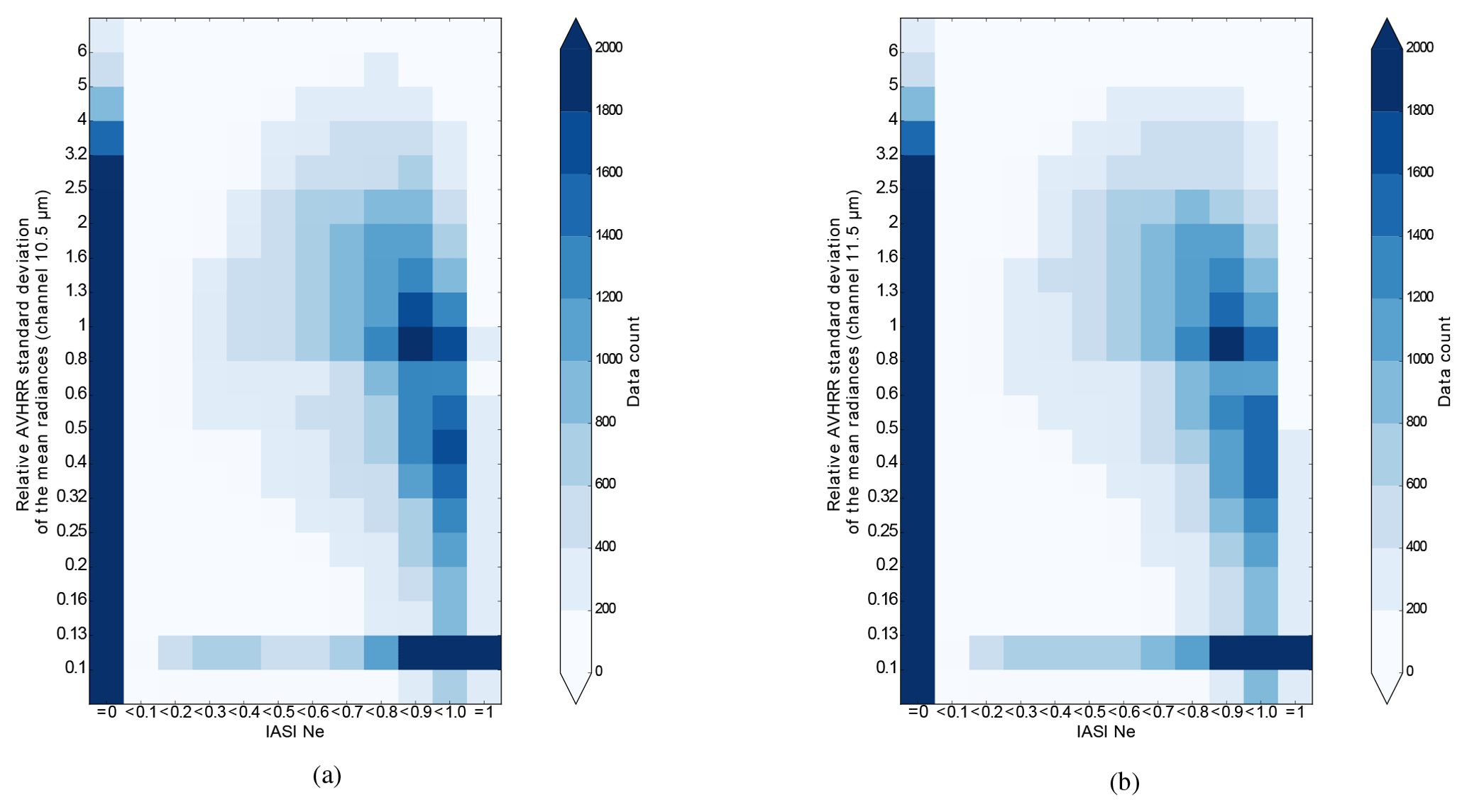
Figure 2 Density plot (number of observations) of the values of effective cloud fraction retrieved from IASI by a CO₂-slicing algorithm (on the abscissa) with respect to the relative cluster standard deviation of the mean radiances (%, on the y axis) for intercluster homogeneity for (a) the AVHRR IR channel (10.5 µm) and (b) the AVHRR IR channel (11.5 µm).

Figure 2 provides a calibration to determine the thresholds to be used to define homogeneous scenes. These thresholds should lead to a sufficient size of the selected dataset and it should avoid selecting the fractional cloud as much as possible. Therefore we decided to select an observation if the ratio between intercluster homogeneity and mean radiance for both AVHRR IR channels (10.5 and 11.5 µm) are less than 0.8 %. This threshold allows us to discard the population of observations with a large cloud cover and a large standard deviation ratio in the top right of the panels. It also allows us to remove some observations for which the CO₂-slicing algorithm has failed to retrieve a cloud-top pressure and for which IASI cloud fraction is set to zero. If this test is only applied over channel 10.5 µm, 68.2 % of the observations are selected, if applied over channel 11.5 µm, 69.6 % of the data are kept and if it is applied over both channels 67.3 % pass the test.

3.2.4 Compromise for the homogeneous scene selection

Based on the previous methods, we propose a fourth one which represents a compromise between them. Both AVHRR infrared channels (10.5 and 11.5 µm) are used, and we define two homogeneity criteria in the observed and simulated brightness temperature spaces.

The first criterion for homogeneity is the interclass homogeneity check which was used in the third method, calculated in the observation space (presented in Sect. 3.2.3). Similarly, we used the background departure check in the observation space D_mean (presented in Sect. 3.2.2).

Only observations that fulfilled both following criteria were selected:

• ratio between intercluster homogeneity and mean brightness temperature for two AVHRR IR channels (10.5 and 11.5 µm) < 0.8 %.

• sum of the average distances between each cluster and the background < 49 K².

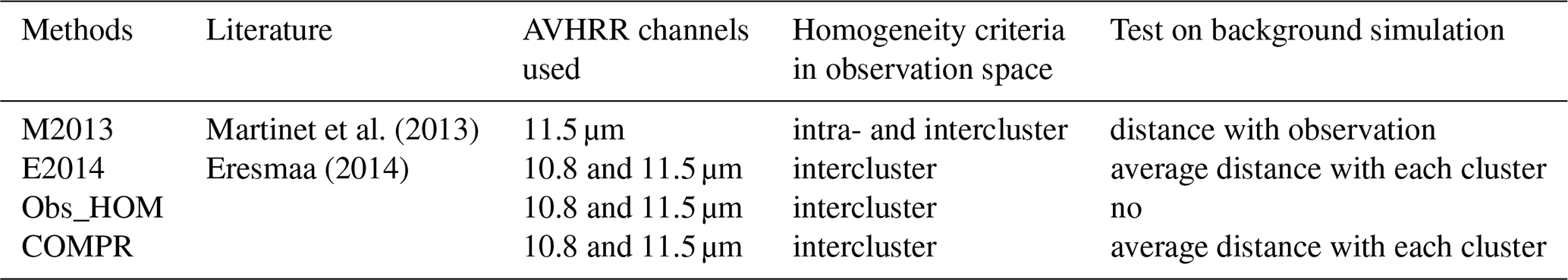
This method is named COMPR in the following. All four methods are summarized in Table 1.

4 Inter-comparison of selection criteria

Martinet et al. (2013)Eresmaa (2014)

Table 1 Summary of the criteria for homogeneous IASI observation selection used in this study.

We applied our selection criteria on 30 January 2017, and results from an observation sample composed of 188 090 IASI FOV during the daytime over the sea are presented. The same conclusions were found in the other cases (night-time and/or over land).

Table 2 Evaluation of heterogeneity inside the IASI pixel with respect to the SEVIRI cloud type.

An evaluation of the homogeneity inside the IASI pixels according to the various selection criteria was performed with independent SEVIRI data over the sea to check that the retained observations are selected for clear or overcast scenes. Here the considered data were the cloud type from the geostationary SEVIRI sounder, which is a product from the Satellite Application Facility in support of NoWCasting and very-short range forecasting of EUMETSAT. For each IASI pixel, the cloud types of the 4 SEVIRI pixels closest to the IASI centre were compared. If the four cloud types were “sea”, the IASI pixel is considered to be clear, if the same cloud type is found in SEVIRI pixels, the IASI observation is set to homogeneous cloudy observation, otherwise it is considered to be a heterogeneous observation. Table 2 presents the results of this comparison. A total of 67 599 IASI observations were collocated with SEVIRI data during the day on 30 January 2017. In the global dataset, we found that 12 % are clear homogeneous observations, 51 % are cloudy homogeneous observations and 37 % of IASI observations are made of different SEVIRI cloud types. This corresponds well to the results obtained with the results found with the percentage of cloudy AVHRR pixels in the IASI field of view (Table 3). When applying the M2013 criteria, 11 % of clear observations are retained. This number does not vary a lot when applying the other criteria. The number of homogeneous cloudy observations is more sensitive to the criteria because it varies between 9 % for E2014 and 35 % for the Obs_HOM one. The COMPR criteria provide a compromise between M2013 ad E2014 in terms of selected observations.

The percentage of cloudy AVHRR pixels in the IASI field was also used to assess the choice of homogeneity criteria (Table 3).

Our global dataset is made of 50 % of the observations entirely covered by clouds and 12 % of clear observations according to the AVHRR cloud cover. These results obtained over the global set agree well with the ones obtained with SEVIRI data over the Atlantic Ocean. The percentage of selected observations for each selection method is larger ($+\mathrm{2}/\mathrm{4}$ %) with the SEVIRI data evaluation than with the AVHRR cloud cover.

The bias and standard deviation of observations minus simulations (O − G), are shown in Fig. 3a for the 314 IASI channels used at Météo-France. As expected, the best statistics are obtained for channels less affected by clouds (e.g. CO₂ and water vapour high peaking channels).

For the whole dataset, window channels present a bias of around −0.6 K. The standard deviations are larger (around 12 K) for window channels sensitive to the surface. With the M2013 selection method (Fig. 3b), the standard deviation of window channels is reduced to around 4 K and the bias reduced close to zero. The standard deviation of the other channels (680–780 cm⁻¹) is also decreased. The E2014 selection method (Fig. 3c) improves the bias and the standard deviation (2.0 K for window channels) for all the channels. As expected, the impact is larger for surface-sensitive (and thus cloud-sensitive) channels than for the tropospheric channels (680–780 cm⁻¹). Conversely, with the Obs_HOM method (Fig. 3d), small improvement of the statistics is obtained for the standard deviation and the bias. The statistics obtained with the COMPR method (Fig. 3e) are reduced compared to the whole dataset and slightly worse than with the initial E2014 method (for window channels the standard deviation is around 2.2 K instead of 2 K for E2014).

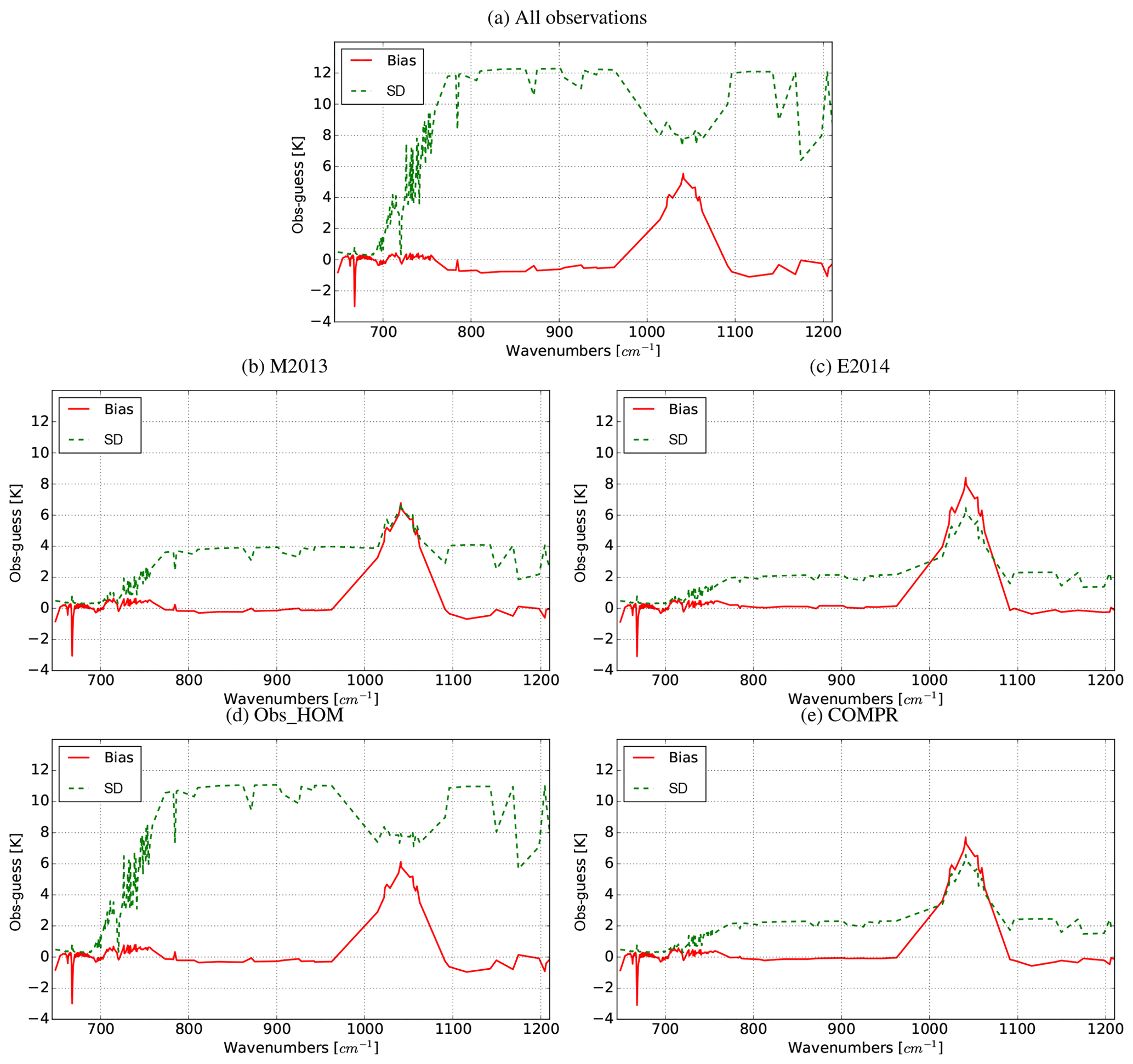
Figure 3 Bias (red solid line) and standard deviation (green dashed line) in kelvin (K) of the differences between IASI observations and background simulations using RTTOV-CLD and a 6 h forecast: (a) for the whole dataset, (b) after applying the homogeneity criteria derived from Martinet et al. (2013), (c) after applying the homogeneity criteria derived from Eresmaa (2014), (d) after applying the selecting homogeneous scenes based on observation space, (e) after applying the compromise to select the homogeneous scenes. Observations are for 30 January 2017.

Table 3 Overview table of statistics obtained with the different homogeneity criteria: number of observations retained, percentage of cloudy observations (cloud cover of 100), percentage of fully clear observations (cloud cover of 0). Percentages are given with respect to all the observations.

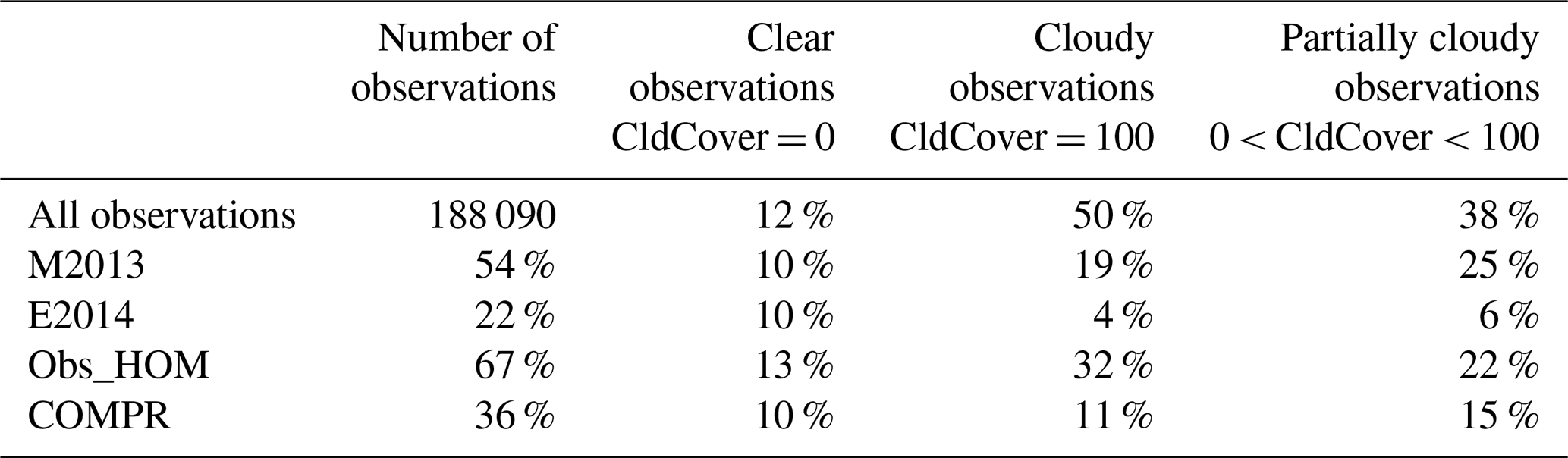
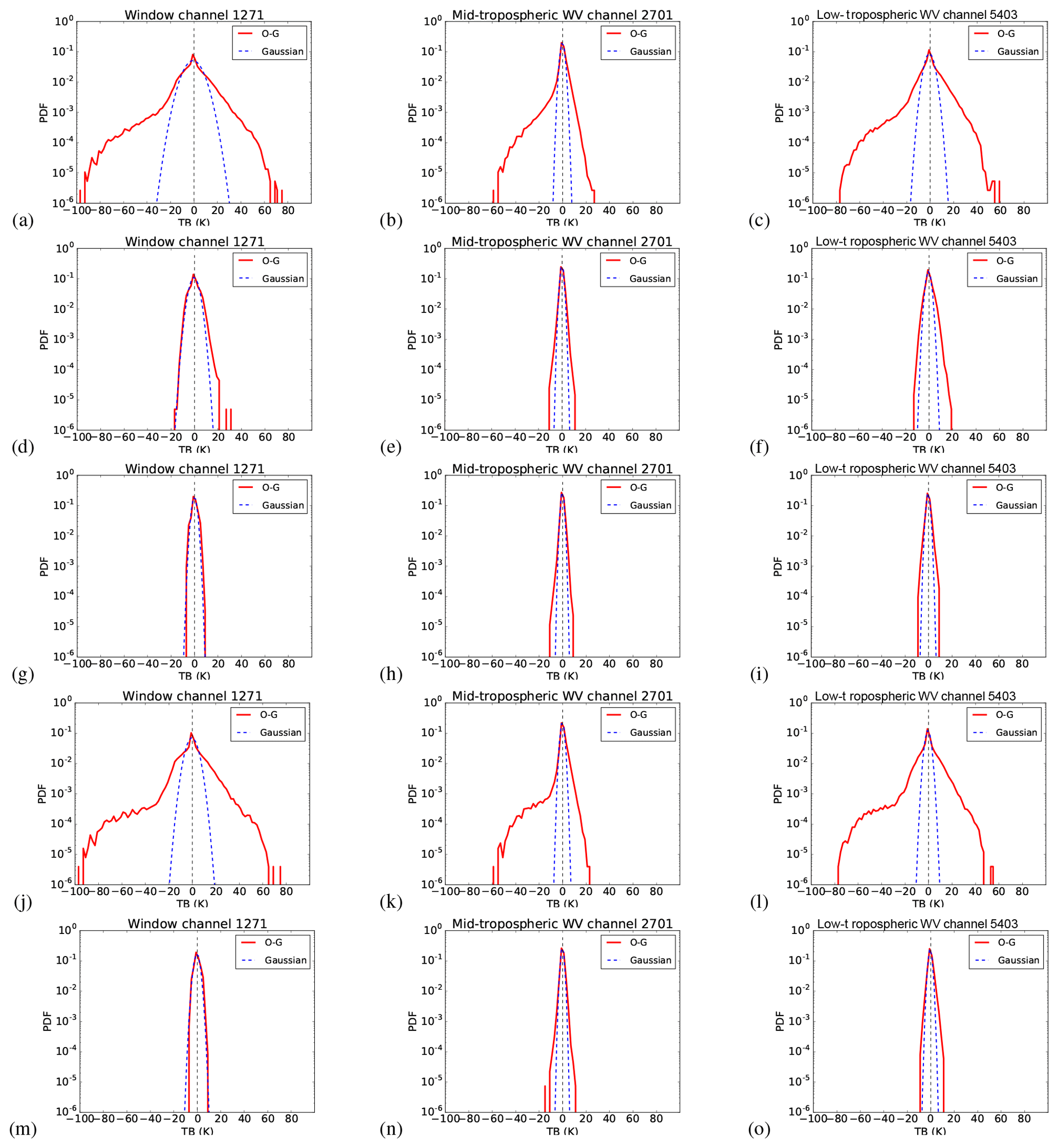
Figure 4 Frequency distribution of brightness temperature difference between observation and background (O − G) for all observations (a, b, c), after applying the homogeneity criteria derived from Martinet et al. (2013) (d, e, f), the homogeneity criteria derived from Eresmaa (2014) (g, h, i,), the third method based on the observation space method (j, k, l) and the compromised approach (m, n, o). The PDFs are presented for three channels: window channel 1271, low-tropospheric water vapour channel 5403 and mid-tropospheric water vapour channel 2701). The Gaussian distributions with the same error characteristics (mean and standard deviation) are also shown as blue dashed lines.

To complete the comparison, the probability density function (PDF) of the O − G differences was studied (Fig. 4). Three channels were assessed: the window channel 1271 (962.5 cm⁻¹, whose weighting function peaks at around 1000 hPa), the mid-tropospheric water vapour channel 2701 (1320 cm⁻¹, weighting function maximum at around 400 hPa) and the low-tropospheric water vapour channel 5403 (1955 cm⁻¹, weighting function peaking at around 900 hPa).

The distribution asymmetry is reduced for mid- and low-tropospheric water vapour channels with M2013 and E2014 selection. The impact of clouds is evident on the window channel, with differences ranging from −90 to 64 K. After the homogeneity criteria have been applied, narrower Gaussian distributions are observed for all channels with a significant improvement for the window channel. Using the M2013 criteria, differences in O − G for the window channel are significantly reduced, from −18 to 20 K, and from −7 to 9 K using the E2014 criteria (Fig. 4g, h, i).

With Obs_HOM criteria (Fig. 4j, k, l), the O − G distribution is not much improved for all channels. When the homogeneity criterion in the model space is added using the COMPR selection, the O − G distributions become symmetrical, get closer to the Gaussian distribution and centre around zero for the three previously selected channels (Fig. 4m, n, o), which indicates the data are correctly diagnosed as homogeneous.

Table 4 Overview table of statistics obtained with the different homogeneity criteria: number of observations retained; bias and standard deviation computed for the channels included in the range between 650–770 and 770–980 cm⁻¹.

Table 4 summarizes statistics in terms of bias and standard deviation of background departure for the different datasets. The bias and standard deviation obtained by the M2013 method have some reasonable statistics before the assimilation (−0.6 K for the bias and 3.7 K for the standard deviation, for the window channels). The E2014 selection method seems relevant for selecting homogeneous scenes in terms of bias and standard deviation (0.11 and 2.0 K respectively, for the window channels). However, the number of selected observations presents a disadvantage for this selection method since the E2014 method keeps only 22 % of the observations, of which 10 % are totally clear, 6 % are totally covered by clouds and 6 % are heterogeneous. These observations are distributed throughout the globe, but we keep more observations on high latitudes.

The Obs_HOM method allows us to keep 67 % of observations, of which 12 % are totally clear and 32 % are totally covered by clouds, but this method does not give acceptable statistics (bias of −0.2 K and standard deviation of 10.5 K). When the test on observations minus simulations of the infrared channels AVHRR is added by the COMPR method, results are improved. For window channels the bias is reduced to −0.09 K and the standard deviation to 2.1 K compared to −0.6 and 11.7 K for all observations, which presents a good score compared to the M2013 and Obs_HOM methods. In addition, 36 % of the observations are retained, compared to the whole dataset, with 10 % clear observations and 11 % cloudy observations of the total, which represents twice the number of cloudy observations selected by E2014, which removes many more observations, and shows that the proposed methodology is effective.

The cloud cover distribution corresponding to the number of observations that is kept (36 %) is made of 28 % clear observations and 29 % observations totally covered by clouds. In addition, 14 % of the observations have a cloud cover of less than 10 % and 4 % of the observations have a cloud cover exceeding 90 %. The observations kept are distributed in different parts of the globe (Fig. 5a), although we have been able to retain different cloud types, including high clouds even in the tropics for a few cases only (Fig. 5b). This may be explained by the weakness of the model clouds in these areas.

Figure 5 Map of IASI observations of brightness temperature (K) for surface channel (1271, 962.5 cm⁻¹), after applying the COMPR method (a), cloud-top pressure (hPa) retrieved from a CO₂-slicing algorithm applied to IASI observations (b), for 30 January 2017 daytime over sea.

The main objective of the study is to select homogeneous IASI observations in clear and cloudy sky, which are well simulated with RTTOV-CLD and could be used in data assimilation. Comparison of different methods of selecting homogeneous scenes showed that the M2013 method improves the first guess departure statistics (bias of −0.16 K and standard deviation of 3.17 K) but it keeps more heterogeneous observations (25 %) accounting for AVHRR cloud cover than the E2014 method, which significantly improves the statistics (bias of 0.11 K and standard deviation of 2 K) and favours more clear observations but keeps only 22 % of the observations. The Obs_HOM method, which focuses only on homogeneity in the observation space, does not strongly improve the statistics, but it filters 33 % of heterogeneous observations. However the addition of the criterion on the simulated observations in the COMPR method improves the scores on IASI simulations (bias of 0.09 K and standard deviation of 2 K) while retaining 36 % of the observations and among them a similar part of homogeneous clear and homogeneous cloudy observations. This data selection representing a compromise between M2013 and E2014 is chosen for a data assimilation experiment.

5 Impact on NWP analyses and forecasts

After the selection criteria were implemented in the assimilation system of Météo-France, their impact was tested through 4D-Var assimilation experiments in the ARPEGE global model. The impact of the homogeneity criteria for data selection on all observation simulations, analyses and forecasts is evaluated.

5.1 Experimental design

To evaluate the impact of our homogeneity criteria on the assimilation process over sea and land, during daytime and night-time, experiments were performed over 1 month from 6 December 2017 to 17 January 2018. A total of 314 IASI channels were used in the simulation, and 129 channels were used for assimilation operationally.

The first experiment is the reference (REF), where IASI observations are assimilated with all other observation types as in the operational system at Météo-France.

In a second experiment called (EXP), we applied our COMPR approach (presented in Sect. 3.2.4) on top of the McNally and Watts cloud detection. As in Eresmaa (2014), these homogeneity criteria are provided for the McNally and Watts detection scheme and applied in its quick-exit scenario. This means that if the COMPR approach flags a homogeneous observation, it can accelerate the decision of flagging the pixel as clear, but if the COMPR approach flags the observation as heterogeneous, the assimilation entirely relies on the McNally and Watts cloud detection scheme to discriminate which channels to assimilate. There is no specific channel set for which the homogeneity criteria are applied. These experiments aim to evaluate the impact of the COMPR method of selecting homogeneous IASI observations on simulation and assimilation processes.

In these experiments, no cloudy observations detected with the CO₂-slicing method and used with a single grey-cloud layer scheme were assimilated, unlike in Guidard et al. (2011). We focus on clear-sky assimilation. RTTOV-CLD was only used to compute the homogeneity criteria based on cloudy AVHRR simulations and RTTOV was used for the clear-sky assimilation.

5.2 Impact on observation

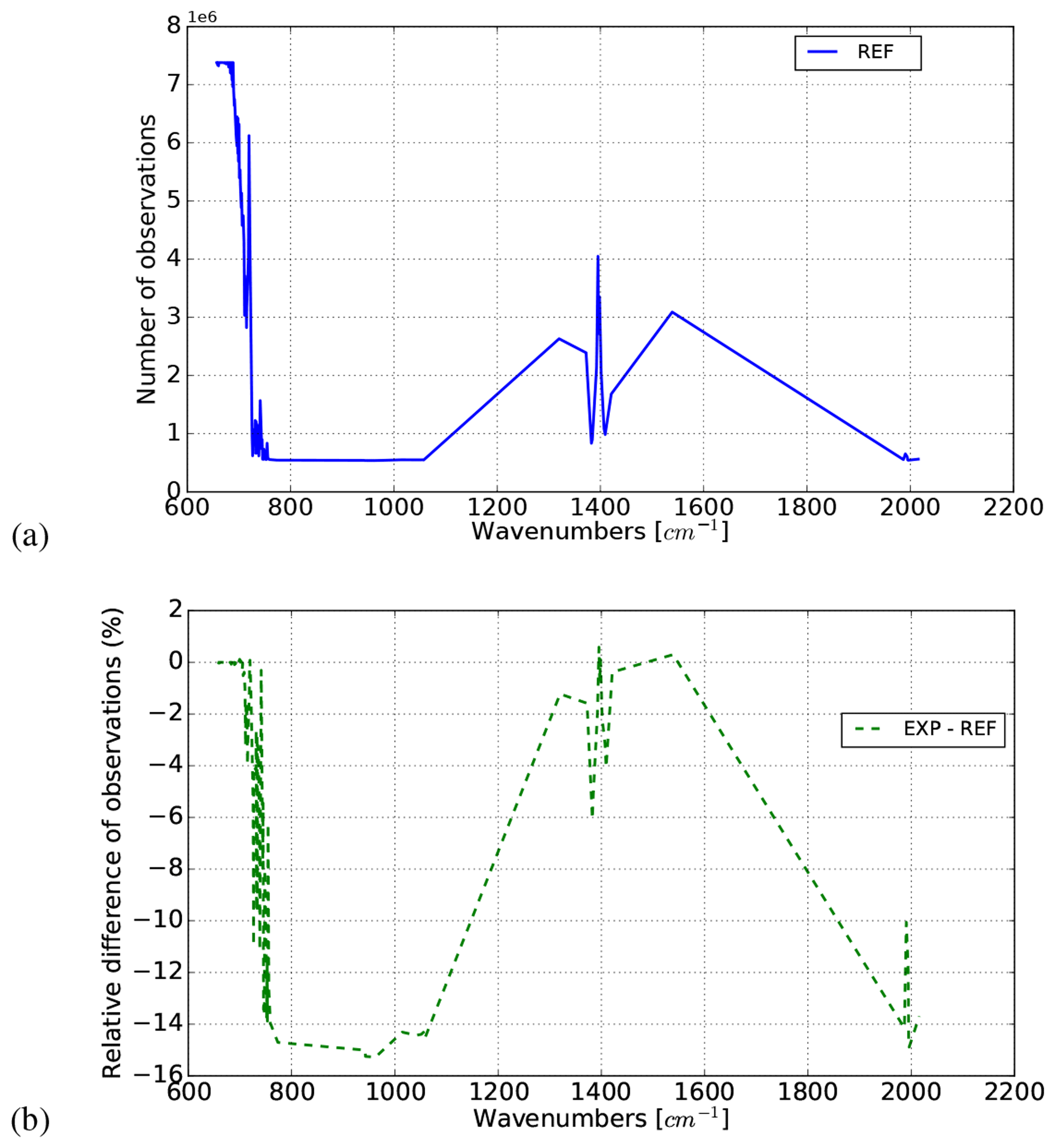
Figure 6 Number of assimilated IASI data over the whole experimental period (41 d) as a function of wavenumber of IASI for the REF experiment (a) and relative difference of number of assimilated observations (b) for the EXP compared with REF (dashed green line).

Figure 6a gives the number of observations assimilated into the ARPEGE model as a function of the IASI wavenumber for REF experiment. This proportion represents around 19.2 % of the total number of IASI observations available for the assimilation. The order of magnitude is below 8.10⁶ for all the wavenumbers considered and for both experiments, showing that among the 129 IASI channels selected for the assimilation, the occurrence proportion is well balanced. However, the number of assimilated channels changes between experiments depending upon the spectral band considered. Four spectral bands can be mentioned:

• -

  [657, 687.25] cm⁻¹ wavenumber range corresponding to the stratospheric temperature channels keeps the same number of observations in both experiments because these channels are not affected by the presence of clouds.

• -

  [726.5, 1421] cm⁻¹ wavenumber range, corresponding to tropospheric and surface temperature channels and also to mid- and high-tropospheric water vapour channels; the number of observations is decreased by 15 % for EXP (Fig. 6b).

• -

  [1800, 2015.5] cm⁻¹, finally the number of low-tropospheric water-vapour-sensitive channels is slightly decreased between 8 % and 14 % for EXP (Fig. 6b).

5.3 Impact on background and analyses

The analysis departure data discussed below are obtained by comparing the analysis between the REF and the EXP experiments to evaluate the impact of the criteria for selecting homogeneous IASI observations.

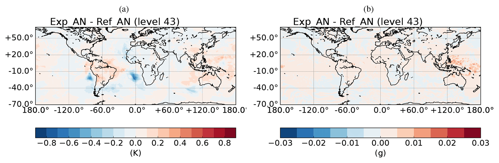
Figure 7 Temperature (a) and humidity (b) analysis difference between REF and EXP for the first assimilation cycle on 7 December 2017 at 00:00 UTC at ARPEGE model level 43, which corresponds to 200 hPa.

Figure 7a and b present the impact of COMPR criteria in the temperature and humidity analyses of the first assimilation cycle. This implementation removes some IASI observations from the assimilation and this reduction has an impact on the analysis. In Fig. 7a, a negative temperature difference is located in the Atlantic Ocean near the southwest African coast. A weaker and patchy impact, which is mainly located in the tropics, is reported on specific humidity. EXP seems to remove some temperature and humidity analysis increments from the REF experiment just at some isolated locations.

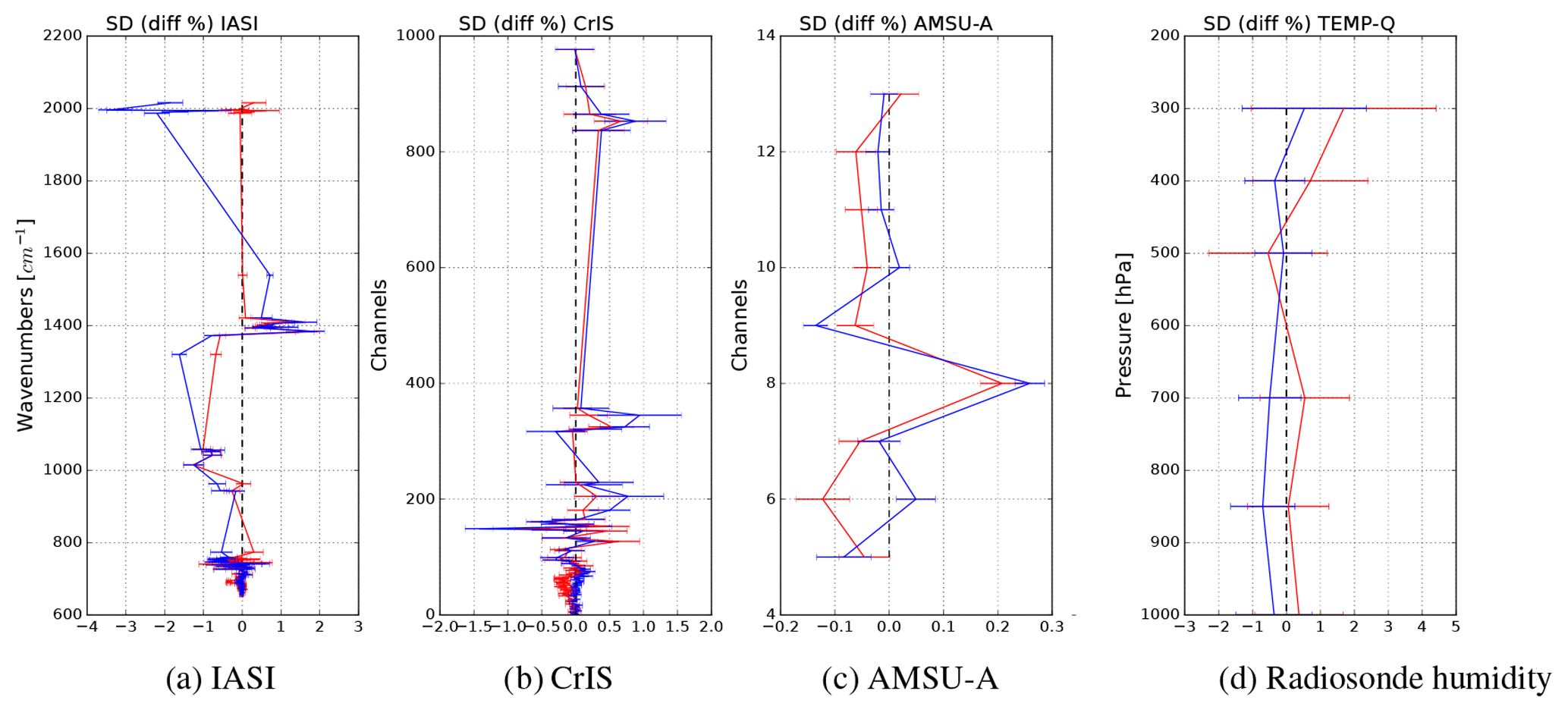
Figure 8 Relative differences of FG departure (red curve) and AN departure (blue curve) standard deviation between EXP and REF for IASI (a), CrIS (b), AMSU-A (c) and TEMP-q (d). The horizontal error bars represent the 95 % significance value for each difference.

In order to assess the impact of the new selection of IASI observations on the analyses and forecast, first guess departures (FG departures) corresponding to the difference between the observations and the simulations from the 6 h forecast and the analysis departures (AN departures) are computed. As biases and standard deviations of FG and AN departures were very weak for IASI, CRIS, and AMSU-A instruments and humidity measurements performed by radiosondes, relative differences have been performed between experiments to highlight detailed comparisons (Fig. 8). Negative differences are related to a reduction of the standard deviation with respect to REF one and thus to an improvement.

For IASI (Fig. 8a), exclusively regarding the significant differences with a 95 % value, the FG departure standard deviation was mainly reduced or unchanged in EXP compared to REF depending upon the wavenumber; increases are observed around 1400 and 2000 cm⁻¹ while significant reduction of 0.5 %–1 % is seen between 1000 and 1320 cm⁻¹. The standard deviation reduction in AN departures can be noted at around 2000 cm⁻¹ and between 950 and 1320 cm⁻¹.

Concerning the CrIS observations (Fig. 8b), the differences are mainly not significant except for water vapour channels CrIS channel 850 where the standard deviation increases for both FG and AN departures and a significant improvement for the AN departures around channel 160.

Results obtained for AMSU-A (Fig. 8c) are mainly satisfactory with FG departure standard deviation differences reduced by around 0.05 % for channels 6, 9, 10, 11 and 12. However, a significant degradation of 0.2 % is observed for channel 8. The AN departure results follow more or less the same behaviour. Finally, no significant standard deviation difference is observed concerning the TEMP-q observations (Fig. 8d).

Results shown in this part report the small but non-negligible impact of the homogeneous criteria implemented into EXP on the analyses and the short-range forecasts. Indeed, as seen in the previous section (Sect. 5.2), selected IASI observations are removed over the most cloudy locations and then they impact the humidity and temperature analyses (as seen in Fig. 7). Statistical results in Fig. 8 report a non-negligible decrease in the dispersion within the FG departure and AN departure for IASI observations and for several channels of AMSU-A but some negative impacts have to be noted for other wavenumbers. More attenuated and mainly non-significant impacts can be recorded for CrIS and TEMP-q observations. Thus, the analyses and short-range forecasts have been slightly changed compared to REF.

5.4 Impact on forecast scores

The forecasts from EXP at 00:00 UTC for the period 7 December 2017 to 17 January 2018 were compared to REF ones and evaluated against radiosondes and operational analyses from ECMWF. Root-mean-square forecast errors at the 12 h forecast ranges with respect to the ECMWF analyses were computed for temperature, relative humidity and wind. Similar computations were made against radiosondes. No major difference can be found between both experiments. Very small improvements of the 12 h forecast with respect to the ECMWF analyses were found in the Southern Hemisphere for temperature and wind at around 700 hPa (Fig. 9). This reduction of 2 % for temperature and 0.5 % for the wind is significant, according to a bootstrap test with a 99.5 % confidence level. Other improvements are found at 200 hPa for temperature (1.5 %) and at 500 hPa for wind (0.5 %). Regarding the evaluation against radiosondes, very small, but not significant, improvements for wind were found in the troposphere in the Southern Hemisphere and in the tropics.

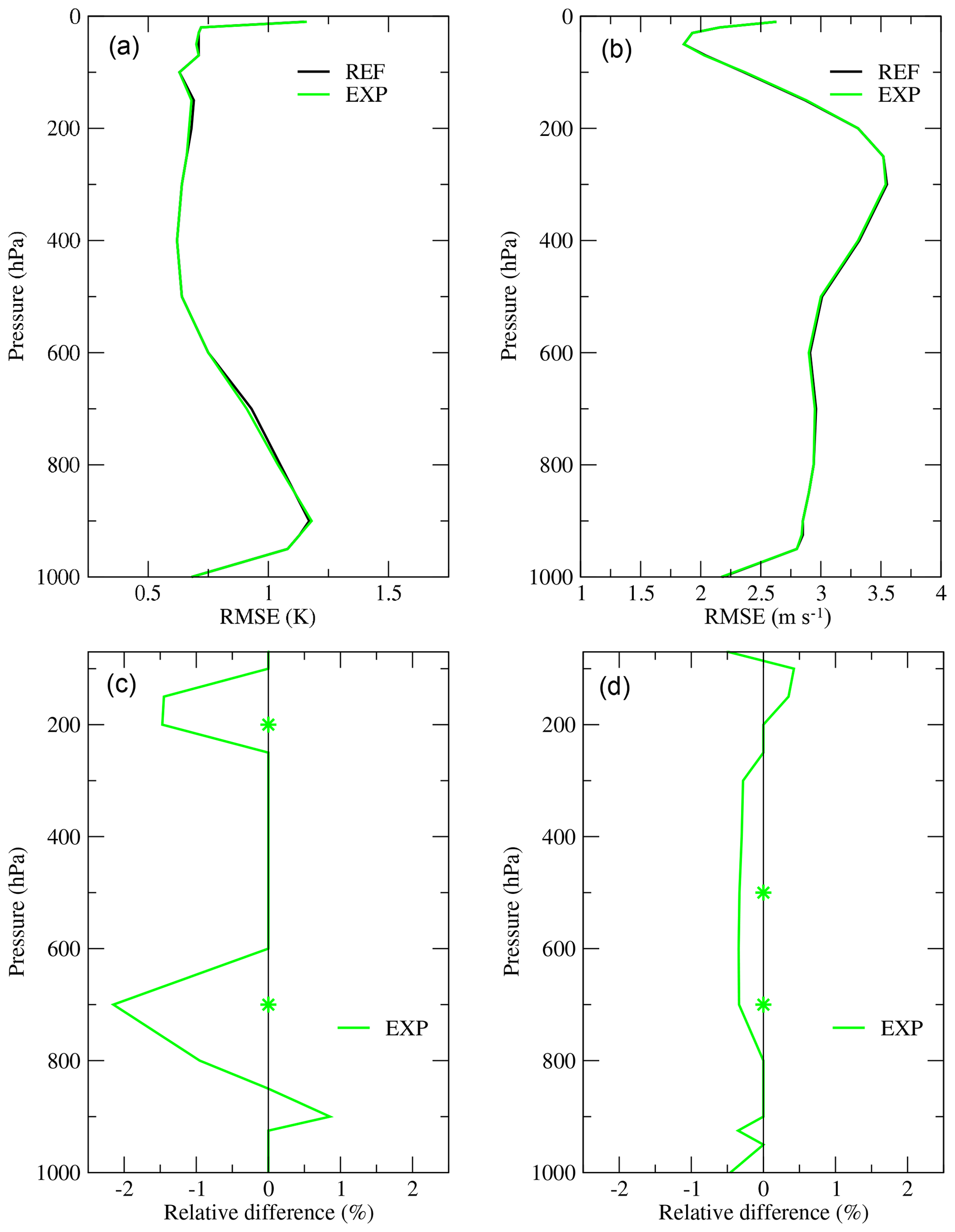
Figure 9 Root-mean-square error of the 12 h forecast error for the Southern Hemisphere computed with respect to ECMWF analyses over the period from 7 December 2017 to 17 January 2018 for REF (in black) and EXP (in green) for temperature (a, c) and wind (b, d). The second line represents the relative difference with respect to the reference. Green stars indicate that the differences of EXP with REF are statistically significant according to a bootstrap test with a 99.5 % confidence level.

6 Conclusion and perspectives

A new method using collocated AVHRR cluster information to improve the selection of homogeneous IASI observation scenes within the numerical weather prediction ARPEGE model has been developed at Météo-France for data assimilation purposes and has been presented in this study.

The first step consisted in adapting the IASI observation operator based on the RTTOV radiative transfer model by using the RTTOV-CLD module with cloudy microphysical parameters (liquid water content (ql), ice content (qi) and cloud fraction) for the simulation of cloudy radiances. A qualitative evaluation of such a module showed realistic simulated cloud structures at various locations around the globe with a quite good agreement against IASI observations.

The second and main step of this work was to assess the impact of several methods used to select homogeneous IASI observations using AVHRR clusters. Two selection methods (derived from the literature: Martinet et al., 2013 and Eresmaa, 2014) were first evaluated. Despite a good improvement in terms of biases and standard deviations of the FG departures, the criteria from the method of Martinet et al. (2013) favour the homogeneous cloudy observations and retain more than a half of the observations, while the method of Eresmaa (2014) gives priority to clear observations and keeps only 22 % of the observations. Then, two criteria were defined from these two previous methods in order to have a more balanced choice of clear and cloudy observations and good statistics in terms of background departures implemented within the ARPEGE model.

• The first criterion derived from the Martinet et al. (2013) method looks for the consistency between different clusters occupying the same IASI FOV by examining this homogeneity relative to the weighted average brightness temperature of the AVHRR clusters; it is only based on observations and computed for both infrared AVHRR channels as in Eresmaa (2014). This criterion allows us to retain 67 % of observations.

• In addition, the second criterion is derived from the test of Eresmaa (2014) and assesses the consistency of each cluster compared to the background brightness temperature simulation; it is in fact a good compromise between the two “historical” ones with accurate statistics and a sufficient number of observations (36 %) that passed the check. It also allows us to retain the same proportion of homogeneous clear and cloudy observations contrary to the derived Martinet et al. (2013) and Eresmaa (2014) methods.

Therefore, assimilation experiments were conducted to assess the impact of these new selections of homogeneous IASI observation features in the current clear-sky assimilation. This revised check was added to the McNally and Watts (2003) cloud detection. The results obtained in this case suggest that the scene categorization has been facilitated and cloudy observations can be better filtered out compared to what is done in the operational ARPEGE version. A total of 1 % of assimilated observations in the reference are rejected with the homogeneity criteria. Depending on the spectral band, up to 15 % of the total number of channels can be discarded with the use of the homogeneity criteria in the assimilation. The number of channels peaking high in the atmosphere (i.e. stratosphere) is not impacted by the homogeneity criteria, as the McNally and Watts algorithm always identifies them as clear. The impacts on the first guess and analysis departures (showing more Gaussian shape) are generally low, but with a beneficial reduction on the standard deviation of first guess departures mainly on the IASI and AMSU-A observations. Regarding the forecast scores, this is a very small positive impact at the 12 h forecast range for temperature and wind in the Southern Hemisphere when these selection criteria are taken into account in addition to the McNally and Watts (2003) algorithm. At longer ranges, neutral impact is found.

However, this step has been necessary to prepare for the future, which will consist of the assimilation of all sky within the ARPEGE model. This method of observation selection allows us to separate the clear-sky and cloudy scenes and manage each route in an independent way. Then, it could be available to directly assimilate the cloudy radiances into the 4D-Var ARPEGE by adapting the observation errors for more cloudy situations. However, hydrometeors used in the RTTOV-CLD are not available in the background error covariance matrix and then cloudy and convective situations are badly represented and will penalize the cloudy direct assimilation. In order to bypass this problem, another solution under study is to retrieve information within cloudy observation using a Bayesian inversion method, in a first step, and to assimilate these retrieved products in terms of temperature and/or humidity profiles into the 4D-Var in a second step. This method, called 1D-Bayesian + 4D-Var, was already studied for microwave radiances (Guerbette et al., 2016; Duruisseau et al., 2018) and has been successfully used since 2010 for radar reflectivity (Wattrelot et al., 2014) assimilation within the AROME convective scale model.