Identification of platform exhaust on the RV Investigator

Oceans cover over 70 % of the Earth's surface. Ship-based measurements are an important component in developing an understanding of atmosphere of this vast region. A common problem that impacts the quality of atmospheric data collected from marine research vessels is exhaust from both diesel combustion and waste incineration from the ship itself. Described here is an algorithm, developed for the recently commissioned Australian blue-water research vessel (RV) Investigator, that identifies exhaust periods in sampled air. The RV Investigator, with two dedicated atmospheric laboratories, represents an unprecedented opportunity for high-quality measurements of the marine atmosphere. The algorithm avoids using ancillary data such as wind speed and direction, and instead utilises components of the exhaust itself – aerosol number concentration, black carbon concentration, and carbon monoxide and carbon dioxide mixing ratios. The exhaust signal is identified within each of these parameters individually before they are combined and an additional window filter is applied. The algorithm relies heavily on statistical methods, rather than setting thresholds that are too rigid to accommodate potential temporal changes. The algorithm is more effective than traditional wind-based filters in removing exhaust data without removing exhaust-free data, which commonly occurs with traditional filters. In application to the current dataset, the algorithm identifies 26 % of the wind filter's “clean” data as exhaust, and recovers 5 % of data falsely removed by the wind filter. With suitable testing, the algorithm has the potential to be applied to other ship-based atmospheric measurements where suitable measurements exist.

1 Introduction

When undertaking atmospheric composition and chemistry measurements, a common issue that impacts data quality is the ability to effectively identify and potentially filter out sources of contamination. The most common local contamination source is often emissions from power generation. Typically, power generation burns hydrocarbon fuels (such as diesel) and emits a range of combustion products that are often the target species being measured in the background atmosphere.

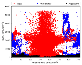
Identification of periods of contamination is performed via a variety of methods depending on the contamination source and the target research question. A commonly used and reasonably reliable method for identification of local point source contaminants is by simple wind direction and speed criteria (e.g. Molloy and Galbally, 2014; Steele et al., 2003; Chambers et al., 2017, and references therein). This method aims to capture the exhaust plume diffusion processes using the two wind measurements as proxies. It is a robust method in environments where background composition is similar to the contamination source, such as in urban areas. However, because of the oversimplified parameterisation, very conservative bounds are often required, which results in the removal of often significant numbers of contaminant-free data. In addition, this method assumes relatively uniform flow characteristics and will fail when atmospheric recirculation results in measurements of contaminated air from directions outside the specified range. Figure 1 exemplifies this issue, where cloud condensation nuclei (CCN) number concentrations are found to be unreasonably high for the marine dataset used here, even after a wind speed and direction filter is utilised.

Figure 1 CCN plotted against wind direction (relative to the platform) from the RV Investigator voyage IN2016_V03. Red: all raw data. Blue: after data are removed when wind speed is less than 5 m s⁻¹ or relative wind directions between 90 and 270^∘. Uncontaminated data are usually less than 1000 cm⁻³ – see Fig. A1. Data filtered with just wind measurements still show clear signs of contamination.

Depending on the environment, a combination of wind criteria and in situ composition measurements can be used to help overcome the recirculation issue. For example, high concentrations of nitrogen oxides (NO_x) produced from combustion processes will react rapidly with background ozone (O₃), resulting in O₃-depleted air, which will only regenerate hours downwind through NO_x chemistry and photolysis processes (World Meteorological Organization, 1985). The use of O₃ can improve wind-based filters to help identify recirculation, depending on the timescale of interest (e.g. Humphries et al., 2015). However, the problem of false-positive identification remains as long as measurements of ancillary data are used for identification. Ideally, identification of contaminated air would use only measurements of species emitted directly by the source itself in order to minimise false-positive contaminant identification and maximise the usable data from a dataset.

In the current study, an exhaust identification algorithm is developed for application to data collected on board Australia's new marine research vessel (RV) Investigator utilising measurements of species emitted directly by combustion processes occurring on the ship – namely diesel combustion and waste incineration. Both combustion processes (hereafter referred to as “exhaust”) have similar emissions relative to the background atmosphere (Reşitoğlu et al., 2015; Johnke, 1999; Jones and Harrison, 2016, and references therein). Emitted species include carbon dioxide (CO₂), carbon monoxide (CO), NO_x, hydrocarbons and high concentrations of aerosols (condensation nuclei, CN), which include those whose composition is primarily black carbon (BC) as well as those that can act as CCN. Measurements of CO, CO₂, BC and CN are utilised for the development of this exhaust identification algorithm as they have clear signals above the background atmosphere and are measured routinely on the vessel.

Figure 2 shows an example period of data from the vessel that illustrates the different signals resulting from exhaust influence that must be characterised in the algorithm. Exhaust influence in CN, CO and CO₂ data is obvious with striking enhancements above variable background signals throughout the sample period. BC data are generally close to zero, with exhaust influence obvious when a signal appears out of the noise. Strong perturbations over extended periods, such as those observed on 18 May, are indicative of direct exhaust influence. Smaller signals, such as those observed in CN data on 19 May, or in BC data on 20 May, indicate a more dilute influence, with sampling likely occurring on the wavering edge of the exhaust plume.

Not all measured parameters respond to the exhaust to the same extent, or necessarily at all. A few examples of this are shown when looking at the time series of the parameters (Fig. 2). Generally when this occurs, a signal is observed in CN data, but is absent in the other species. This is likely a result of the magnitude of differences in exhaust signal in each parameter, as well as sensitivity of the measurement techniques of the different species. Figure A1 clearly shows the magnitude differences of the various instruments with exhaust strikes. Exhaust strikes in CN are observed as perturbations of almost 4 orders of magnitude, while those in BC, CO and CO₂ are factors of 10, 0.2 and 0.01, respectively. Being a simple counting instrument, the condensation particle counter (CPC) is sensitive to particle concentrations down to 1 cm⁻³. For the CO and CO₂ measurements, although precision is high, the flow-through-cell technique utilised results in physical integration of the sample over a minute, thereby smoothing out any perturbations. For BC measurements, the detection limit of the instrument is 0.05 µg m⁻³ over a 10 min average. At 1 Hz time resolution, we are still able to get a useful signal (for the current purpose) at 0.01 µg m⁻³ mass resolution; however the instrument is clearly missing significant exhaust influence.

The RV Investigator is a blue-water research vessel capable of traversing from the ice edge to the Equator. The types of atmospheres it encounters range from pristine background, to continental (e.g. while sampling near the coast), to urban environments (e.g. while in port). An important objective of this algorithm is the ability to distinguish the local ship exhaust from the atmosphere of interest – a task which becomes particularly difficult in the more polluted environments such as those downwind of large urban centres. In this study, the dataset utilised for development contains influences from urban and background marine regions (as shown in Figs. A2 and A3) by which differentiation from ship exhaust can be achieved. The ship track of the utilised voyage is shown in Fig. A4.

In this study, an algorithm is developed that produces an exhaust identification product that is published alongside other publicly available datasets from this platform. The algorithm aims to accurately identify exhaust from the ship itself, distinct from other polluted atmospheres such as urban centres, and minimise false-positive identification in order to retain as much valuable data from this mobile platform as possible. The exhaust product is developed utilising a dataset exemplifying the range of atmospheres that are sampled and is validated by applying it to measurements of CCN that were measured simultaneously.

2 Instrumentation

The RV Investigator (schematic shown in Fig. A5) is a state-of-the-art research platform commissioned in 2015 by the Australian government. The vessel is designed for blue-water research and is capable of spending up to 300 d per year at sea, with a single voyage up to 60 d and over 10 000 nautical miles. Propulsion and power are provided by two diesel–electric engines together with three 3000 kW, nine-cylinder diesel engines. Exhaust from diesel combustion, together with waste incineration, which is emitted from a separate but co-located flue, provides the largest source of contamination to atmospheric measurements aboard the platform.

The vessel has been purpose built with two dedicated atmospheric laboratories along with a custom-designed air sampling inlet located above the ship's bow, approximately 18.4 m above sea level. The aerosol laboratory is situated directly underneath the air sampling inlet fore of the anchor well, such that the distance between sampling and instrumentation, and thus sample losses, is minimised (total distance to the aerosol laboratory's sampling manifold is ∼8 m). The aerosol laboratory houses instrumentation for the measurement of aerosols and the reactive gas ozone. The air chemistry laboratory is situated further aft in the vessel at the fore of the superstructure (total distance from main sample inlet to the air chemistry laboratory's sampling manifold is ∼38 m), and houses instrumentation for the measurement of less reactive atmospheric species such as greenhouse gases and volatile organic compounds.

The RV Investigator houses a range of permanent instrumentation. These instruments are run continuously throughout every voyage of the RV Investigator (except for when instruments are removed for maintenance or faults) and after data have been calibrated, and quality assurance and control procedures have been performed, data are made publicly available. Of particular relevance to this study is the measurement of CO, CO₂, BC, CN and meteorological measurements. Each of these parameters will be described in detail in future publications documenting the ongoing measurements of the vessel; however a brief overview of these measurements is given here. For this analysis, CCN data are utilised as an independent parameter by which the exhaust identifier is tested. The dataset considered in this paper utilised CN and CCN data captured by instrumentation deployed specifically for this voyage, and thus will be described separately. It is worth noting that both CN and CCN instrumentation have more recently become part of the permanent ongoing instrument suite and will be described in a future publication and made publicly available alongside other aerosol data from the platform.

An important outcome of the current work is to make publicly available an exhaust identification data product that will be published alongside other atmospheric datasets from the vessel in order to assist data users in their analyses. For the present paper, the exhaust identification product has been developed using data from the RV Investigator voyage IN2016_V03 (see Marine National Facility, 2016, for voyage track), and data utilised and produced in this paper are available from Humphries et al. (2018).

2.1 Carbon monoxide, CO

Mixing ratios of carbon monoxide (CO) were measured continuously at 1 Hz using a mid-infrared (IR) quantum cascade laser spectrometer (Aerodyne Research Inc, Billerica, MA, USA). A high-vacuum dry scroll pump (model SH-110, Varian, Lexington, MA, USA) draws air through the 0.5 L optical cell maintained at a constant pressure of 6 kPa, and flushed at a rate of approximately 0.5 L min⁻¹. Mid-IR laser light enters the astigmatic multi-pass cell, traversing it 238 times, giving an effective path length of 76 m. Upon exit from the optical cell, the light impinges on a thermoelectrically cooled IR detector, allowing a mixing ratio to be determined via Beer's law. The nominal precision of the CO measurement is 60 ppt in 1 s (owing to the long-path length and strong transition of the CO molecule in the mid-IR). Water vapour is also measured, allowing for the CO mixing ratio to be corrected to a dry air mixing ratio, without the need to pre-dry the sample.

2.2 Carbon dioxide, CO₂

Atmospheric mixing ratios of carbon dioxide (CO₂) are measured continuously at 1 Hz on board the RV Investigator using a Picarro cavity ring-down spectrometer (model G2301, unit CFADS2315, Picarro Inc., Santa Clara, CA, USA) that concurrently measures methane (CH₄) and water vapour. Air is drawn through the 35 sccm optical cell held at constant temperature and pressure (45 ^∘C and 19 kPa), at a rate of approximately 0.15 L min⁻¹. The ends of the cell comprise highly reflective mirrors that recirculate the light supplied by a near-infrared (NIR) laser through the cavity, resulting in an effective path length of around 20 km. Light leaks out of the mirrors, impinging on a photodetector with a characteristic ring-down time. Carbon dioxide molecules within the cell also absorb a fraction of the light, modulating the ring-down time in proportion to their concentration. By scanning the laser off the absorption peak and remeasuring the ring-down time, the technique becomes insensitive to fluctuations in laser power. The precision of the CO₂ measurement is better than 0.05 ppm at a minute average. Data used in this paper are raw CO₂ dry air mixing ratios (by an empirical correction using the native water vapour measurement). CO₂ data are also available as minute and hourly mean dry air mixing ratios that have been calibrated and drift corrected through the daily measurement of a reference tank.

2.3 Black carbon, BC

Black carbon measurements are made using a multiangle absorption photometer (MAAP model 5012, Thermo Fisher Scientific, Air Quality Instruments, Franklin, MA, USA). The MAAP collects aerosol on a glass fibre tape that gets irradiated with 670 nm light. Photodetectors measure the light transmission and reflection in the forward and back hemispheres, respectively, and after inversion, report black carbon concentrations in real time. The inversion algorithm takes into account multiple-scattering processes inside the aerosol sample and between the sample and the filter matrix and utilises a carbon mass absorption coefficient of 6.6 m² g⁻¹. The detection limit of the instrument was calculated by choosing an exhaust-free period (midnight 23 April to 18:00 UTC (for all times) 25 April) in the deep Southern Ocean, where sources of BC are absent other than the platform exhaust. At 1 Hz, the detection limit was calculated to be 0.05 µg m⁻³. The choice of an appropriate threshold must be performed carefully with this detection limit in mind, and is discussed further in Sect. 3.1.

2.4 Aerosol number concentration, CN

Number concentrations of condensation nuclei larger than 3 nm (CN) were measured continuously at 1 Hz using a condensation particle counter (CPC model 3776, TSI Inc., Shoreview, MN, USA). The CPC works by drawing the aerosol sample continuously through a chamber of supersaturated 1-butanol, which condenses onto particles larger than 3 nm, growing them to sizes (above 1 µm) which can be counted individually by a simple optical particle counter. Sample flow rate is regulated by a critical orifice at 1.5 L min⁻¹. This flow rate was checked every few days at the instrument inlet using an external flowmeter (Sensidyne Gilibrator, St. Petersburg, FL, USA) and flow rates were found not to deviate beyond 1 %. Although flow calibrations were not necessary for this algorithm, the software used for filtering the data simultaneously performs flow calibrations, so calibrated data are used here. Data are also filtered for periods of instrument zeros and the disconnection of the instrument from the sampling line. Note that for voyages after September 2016, a permanent CPC (model 3772, TSI, Shoreview, MN, USA), measuring CN larger than 10 nm, was installed on the platform (described in detail in future publications) and is used as the CN data stream.

2.5 Cloud condensation nuclei, CCN

Number concentrations of cloud condensation nuclei (CCN) were measured continuously at 1 Hz using a continuous-flow streamwise thermal-gradient CCN counter (CCNC, model CCN-100, Droplet Measurement Technologies, Longmont, CO, USA). The instrument was situated at approximately the same distance from the inlet as the CPC, connected to the manifold using a combination of stainless-steel and flexible conductive tubing. The instrument was configured to run continuously at 0.5 % supersaturation, which after pressure calibrations, was found to equate to 0.5504 % supersaturation. The flow rate of the instrument was set to the standard 0.5 L min⁻¹. Flows were checked weekly using an external flowmeter (Sensidyne Gilibrator, St. Petersburg, FL, USA) and concentrations were corrected in post-processing procedures based on actual flow rates (maximum of 2 % flow deviation). Data were quality controlled by removal of periods during which maintenance was performed and calibrated for pressure and flow rates.

2.6 Meteorological data

Meteorological data were measured continuously whilst the ship was underway. Meteorological measurements include air temperature, relative humidity, barometric pressure, solar radiation, precipitation, sea surface temperature, wind speed and direction. Of particular interest to the exhaust filtering algorithm are measurements of wind speed and direction. Dual wind monitors (Marine Wind Monitor, model 05106, R.M. Young Company, Traverse City, Michigan, USA) are affixed to the vessel's foremast at a height of 24 m from the water line, each offset from the ship's centreline by ∼2.5 m, one to starboard and the other to port. The measurable wind speed range of the wind monitors is 0–100 m s⁻¹ (±1 %), with an azimuth range of 0–355^∘ (±3^∘; relative to ship centre line; the 5^∘ dead zone of which is directed aft). An ultrasonic two-axis anemometer (WindObserver II, Gill Instruments, Lymington, Hampshire, UK) is also affixed to the foremast 21 m from the water line and ∼2.5 m to port from the ship's centreline. The ultrasonic anemometer measures wind speed in the range 0–65 m s⁻¹ (0.01 m s⁻¹ resolution and ±2 % at 12 m s⁻¹) and azimuth range of 0–359^∘ (1^∘ resolution and ±2 % at 12 m s⁻¹). Wind sensors are calibrated annually by Ecotech Australia to the reference standard ISO 17713-1:2007.

3 Exhaust identification

The primary task of the algorithm is that of distinguishing between two distinctly different signals in our data. Because of the magnitude of the difference, a first pass of the exhaust identification is simply an application of outlier detection algorithms. However, on closer inspection, the variability of the exhaust signal due to variations in source strength, dilution and plume location sampling, as well as the shear length of time that the exhaust can influence measurements (from seconds to days), makes many of the more well-known detection algorithms unsuitable to this problem. This is discussed more in Appendix Sect. A where a number of algorithms, including fast Fourier transform, z score and modified z score, double exponential smoothing, and histogram methods, were tested and found to be unsuitable. Hence this complicates the goal of the algorithm to differentiate between these two distinct but varying signals (i.e. exhaust and ambient in a range of environments).

Exhaust identification is performed primarily utilising the intersection between four parameters commonly emitted in fossil fuel combustion processes, namely CO, CO₂, BC and CN. Figure 2 shows the variability of these species during periods of exhaust influence and within background air (defined here as not influenced by exhaust from the measurement platform, the RV Investigator). Distinct signals are observed in all four variables; however it is important to note that not all signals respond simultaneously. This concept is discussed in detail later in the paper.

Because of the differences in their exhaust responses, identification is performed on each of the parameters separately at 1 Hz, after which they are combined (aligned by time) and an additional window filter is applied to remove neighbouring values that are not captured completely by the parameters themselves. Each instrument connected to the Investigator's sampling system will also exhibit temporal variations in their responses to exhaust strikes due to differences in residence and detector response times. Because of this, it is impossible to create a single exhaust identification product that can be applied to every instrument that collects data on this platform. To effectively achieve a perfectly exhaust-free dataset for each instrument without removing substantial data that are free from exhaust, identification should ideally be performed on each dataset individually. Nevertheless, the creation of this exhaust identifier product is useful in that it creates a first-pass filter that identifies the vast majority of the exhaust influence. With this in mind, a relatively conservative approach is adopted in order to strike a balance between not identifying periods of exhaust influence, and the false-positive identification of background data as exhaust. Since the product is not used to filter published datasets, but instead is published alongside other data, it is left to the end user to determine whether more stringent criteria should be applied to specific datasets than the relatively conservative approach adopted here.

3.1 BC threshold filter

In the background atmosphere, BC is generated from combustion sources such as fossil fuel burning and biomass burning (Seinfeld, and Pandis, 2016). Moreover, the lifetime of BC is on the order of days (Cape et al., 2012) and combined with transport dilution, seeing elevated values beyond the instrument sensitivity is rare. This is illustrated in Fig. A3 where the baseline trend observed in CN during a period of urban influence (26 May) is absent in the BC data. Consequently, a set threshold value can be utilised for BC, whereby any data above this threshold are identified as exhaust.

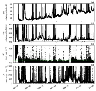
The threshold for exhaust was determined by selecting numerous periods when background air was being measured without exhaust influence, and selecting the maximum value during these periods. For the dataset being utilised for this paper, a value of 0.07 µg m⁻³ was chosen, which is suitable for remote locations and above the detection limit. Figure 2 shows one such period when the ship was located southeast of New Zealand in the deep Southern Ocean. For most voyages undertaken by this vessel this BC limit is suitable; however when the scientific questions are concerned with air masses downwind of major pollution sources, such as urban centres or significant biomass burning events, this limit should be increased. This is illustrated in Fig. A3 where the first week of June shows increased baseline values of CN and also BC due to the vessel coming into and out of the port in Wellington, New Zealand. If these periods were of particular interest, and the data loss from the standard limit was unacceptable, a new increased limit would need to be determined by choosing a period representative of the scientific outcome. Alternate statistical methods, such as choosing a limit based on the 95th percentile or similar scheme, are not generally suitable for the choice of the limit since these generally rely on “outlier”-type data, rather than what is observed here.

3.2 Variance filter for CO, CO₂ and CN

In contrast to BC, CO, CO₂ and CN all have persistent, non-zero background signals in the atmosphere and consequently a simple threshold filter cannot be utilised. For these datasets, the variability is characterised on each dataset and outliers in the positive direction are identified as exhaust. As discussed by Leys et al. (2013), the robust statistical parameters of median and median absolute deviation (MAD) are useful in the detection of outliers since they are relatively insensitive to outliers compared to the mean and standard deviation (SD) that are commonly utilised.

For a univariate dataset $x_{\mathrm{1}},x_{\mathrm{2}},\mathrm{\dots },x_n$, the MAD is defined as the median of the absolute deviations from the data's median:

$$\begin{array}{}\text{(1)}& \mathrm{MAD}=\mathrm{median}\left(\right|x_i-\mathrm{median}\left(x\right)\left|\right).\end{array}$$

It is well established that for normally distributed data (such as is being explored here for data without exhaust), the median and mean are equivalent. The same can be said for the MAD and the SD provided a standard factor is applied (Rousseeuw and Croux, 1993, and references therein) such that

$$\begin{array}{}\text{(2)}& \mathrm{SD}=\mathrm{1.4826}\times \mathrm{MAD}.\end{array}$$

To identify the exhaust, the data point in question must be assessed to determine if it is within an acceptable range that represents the background atmosphere. Defining this acceptable range deserves thoughtful consideration. Given the variability of CO, CO₂ and CN in the background atmosphere, a predefined range would not be fit for purpose. This circumstance lends itself naturally to the use of a rolling window. For this algorithm, numerous statistical parameters (median, MAD and SD) are calculated on a detrended, centred rolling 5 min window. Although variable, the 5 min width of this rolling window is chosen here so that there are enough data for statistical robustness, yet short enough to capture real changes in atmospheric state.

It is important to note that when the fraction of outliers dominates (>50 %) a sample (or window), median-based statistics also become sensitive to outliers. This will happen when, for example, the rolling window is sampling during an exhaust period that persists longer than half the window period. To get a statistical dataset that represents the background atmosphere to which raw data can be compared, alternative values must be sought during these periods when all calculated statistics are affected.

The first step in this process is to identify periods when median-based statistics are affected in the rolling window. Comparing the rolling SD (SD_i) and MAD (MAD_i) could be effective for identifying these periods since one is sensitive to outliers while the other is not, respectively. However, since the exhaust could represent up to 100 % of the sample window, the rolling MAD (MAD_i) and SD (SD_i) could be similar, ruling out comparing these two parameters as a method for identification. To overcome this, a single MAD value (MAD_B) that is representative of the background atmosphere is sought to which we can compare SD_i.

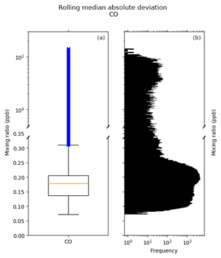
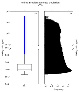
Analysis of CN, CO and CO₂ data shows that MAD_i are generally tightly grouped, but have a small fraction of large outliers, as shown in Figs. A6, A7 and A8. Choosing the median of this MAD_i dataset, MAD_B, yields the value representative of the background atmosphere to which SD_i can be compared and exhaust-affected median statistics can be replaced. Time periods with SD_i larger than 3 times MAD_B are then flagged and values during these periods are replaced with values obtained by linear interpolation with neighbouring values, yielding new datasets, $M_i^{\mathrm{B}}$ and ${\mathrm{MAD}}_i^{\mathrm{B}}$, that represent the rolling median and MAD without influence from exhaust. Having obtained statistical datasets reasonably free from exhaust influence, exhaust can be identified in the raw data such that

$$\begin{array}{}\text{(3)}& x>M_i^{\mathrm{B}}+\mathrm{3}{\mathrm{MAD}}_i^{\mathrm{B}},\end{array}$$

where x is the raw CO, CO₂ or CN data.

The algorithm only identifies positive deviations as exhaust, ignoring negative outliers. This is done because the exhaust can only add signal to the background for these three parameters at this range and at this high frequency. Inclusion of the lower limit could erroneously identify exhaust time periods which are simply instrument zeros or calibrations that may not have been removed from the datasets prior to their use in the algorithm.

The use of uncalibrated and uncorrected CO, CO₂ and CN data is acceptable within the algorithm so long as periods of instrument calibrations in the positive direction are removed from the datasets prior to use (only positive since the exhaust influence on these parameters are all in this direction). This is because the algorithm is sensitive to high-frequency changes like exhaust strikes or instrument zeros, rather than lower-frequency variations, such as instrument drifts, and takes no account for the absolute value of the signal.

3.3 Window filter

Once identified by either CO, CO₂, BC or CN, separate data streams are aligned on the time dimension and a combined exhaust identifier is created such that exhaust is present if detected by any of the four parameters. To this dataset, a window filter is applied. This rolling filter sums the number of exhaust points in the window. If this sum is larger than 10 % of the number of points in the window, then all data points within that window are labelled as exhaust. The 10 % threshold is important because variations in one of the three parameters (arising from the use of raw data streams) could mistakenly identify a time period as exhaust without verification from either sustained exhaust identification or other parameters. Additionally, this 10 % threshold, together with the choice of the window width (here set to 20 min), creates a buffer that accounts for differences in residence times of atmospheric samples in the sample lines and in the instruments themselves (the greenhouse gas measurements are approximately 40 m downstream of the aerosol measurements, resulting in time differences on the order of seconds, compared to the window width, which is several orders of magnitude larger).

4 Results and discussion

Figure 2 shows a subset of data to illustrate the exhaust filter when applied to the CCN dataset. CCN are used here as an independent dataset to test the exhaust filter algorithm and ensure its applicability beyond the parameters used in the algorithm itself. In addition, exhaust strikes are easily visible in the CCN dataset, making it useful for this purpose.

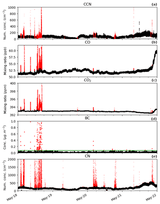
Figure 2 A 4 d subset of the data from the 2016 voyage used to illustrate the algorithm, with filtered data (black) shown atop the raw data (red). Panel (a) shows the unfiltered CCN data along with data after the full filter is applied. Panels (b) to (e) show the filter parameters as both raw and with their individual filters applied. The green line in (d) represents the BC limit of 0.07 µg m⁻³ utilised. All data are raw instrument output without calibrations to aid in rapid dissemination of the exhaust identification product. Timestamps are UTC. Note that y axes are limited in range to reveal baseline values (full data shown in Figs. A2 and A3). Exhaust signal for CO, CO₂, BC and CN extends up to 800 ppb, 490 ppm, 10 µg m⁻³ and 10⁶ cm⁻³, respectively.

Although not 100 % effective, the algorithm removes the vast majority of exhaust influence and its effectiveness, particularly compared to other methods, is clearly apparent (Fig. 2). It is clear from Fig. 3, where each parameter of the filter is applied separately, that none of the parameters are capable of entirely capturing the exhaust influence individually. The CN filter is the most effective, presumably because the exhaust signal is orders of magnitude higher than background values and the response time is rapid. Nevertheless, a significant fraction of exhaust periods make it through the CN filter. When all parameters are used together, the exhaust filter improves dramatically, although a small fraction of exhaust values remain. The application of the window removes most of the remaining exhaust-affected data, resulting in a dataset that can be confidently used in subsequent analyses of the background atmosphere.

Figure A9 shows different combinations of the individual filters to demonstrate the effectiveness of each filter. Combining both Figs. 3 and A9 indicates that CN is the most effective parameter, followed by BC, CO and CO₂. By itself, CN removes the vast majority of the exhaust influence, but alone is incomplete. While this suggests that a simple filter utilising CN and only one of the other three parameters could be used to produce a similarly effective filter, in practice, having all three measurements (i.e. BC, CO and CO₂) provides important redundancy. Currently, if problems occur with the CN measurements, the effectiveness of the exhaust filter is significantly reduced, as shown by Fig. A9h. Given the importance of the CN data to being able to effectively identify exhaust, instrumental redundancy for CN measurements is an important feature of the platform that is currently being implemented.

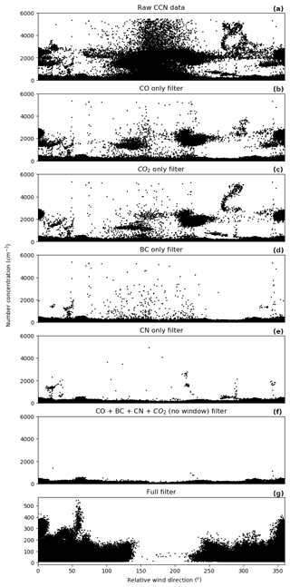
Figure 3 CCN data (linear scale) with the different steps of the algorithm applied separately: panel (a) shows unfiltered data, panels (b) to (e) show single-parameter filters, panel (f) shows the combination of the four parameters, and panel (g) shows the full filter, which includes all parameters and the application of a window removal. Note the change in scale of the y axis in the final panel.

Interestingly, there are some periods which still show short periods of exhaust in the filtered CCN data, as shown in Fig. A10. Here, the exhaust is easily identified by the CN filter algorithm; however after applying the exhaust to the time-synchronised CCN data, the exhaust signal is delayed in the CCN data by about 10 s, presumably due to the longer residence time of the CCN instrument. It is possible to alter the algorithm in such a way that the 20 min window applies to any period identified as exhaust (rather than having the threshold described in Sect. 3.3); however this has the immediate ramification of large losses of data that would otherwise be classified as background, which would be unacceptable for this purpose. Instead, this exhaust identifier has been designed to be used as an initial step, and if more stringent bounds are required by the end user, a more strict window filter can be applied at that time. In addition, individual datasets should be analysed for any remaining exhaust to account for differences in residence time and sampling regimes.

Application of the algorithm to other atmospheric datasets is an important verification step beyond that of CCN, which is a very similar measurement to that of CN measurements. In Fig. A11, aerosol size distributions, measured using a scanning mobility particle sizer (GRIMM SMPS model 5.420 with M-DMA installed, GRIMM Aerosol Technik, Ainring, Germany), are shown as raw data, as well as with both the wind-based filter and the exhaust algorithm applied. Both filter methods are effective at removing much of the exhaust influence; however the exhaust algorithm shows distinct advantages for more accurate exhaust identification, recovering more exhaust-free data and removing exhaust-laden data compared with the wind filter.

Comparison of the algorithm to the traditional wind-based filter shows significant advantages. When applied to this dataset, the algorithm is able to recover 5 % (1 h) of data that the wind filter identified as exhaust, and removes 26 % (37 h) of data that the wind filter identified as clean. This is shown most clearly in Fig. 4 (also apparent in Figs. A12 and A13). Data recovery is obvious in this figure from data present between relative wind directions of 90 and 270^∘, while the high concentrations observed outside these ranges, which are exhaust signal, is removed by the algorithm. From the time series case study of Fig. A12, it can be seen that many of the exhaust signals missed by the wind filter are those on the edges of a large exhaust period, or simply just small exhaust strikes that might occur when the ship is turning.

Figure 4 As in Fig. 1, but with the addition of CCN data filtered using the algorithm described in this paper. The algorithm is significantly more effective than the traditional wind-based filter.

5 Conclusions

A ship exhaust identification algorithm is described that utilises only components of the combustion exhaust, rather than commonly utilised ancillary data such as wind speed and direction. CO, CO₂, BC and CN data are used as exhaust indicators and together with surrounding time-window removal, a robust exhaust identification method results. Statistical methods feature heavily in the algorithm in order to avoid, as much as possible, cut-off thresholds that can be subjective. The algorithm exhibits significantly improved performance compared to more traditional filters, identifying all of the exhaust periods (26 % of data identified as clean by wind filters were identified as exhaust by this algorithm), as well as recovering data falsely identified by other overzealous or indiscriminate methods (the algorithm recovered 5 % of data that wind-based filters removed), thereby optimising usable data. The algorithm is applied directly to data from the RV Investigator for which it was specifically developed and the resulting data product will be made available alongside other publicly available data from the research platform.

Appendix A: Outlier detection algorithms

Due to the magnitude of differences between the exhaust air and ambient air, exhaust can in the first instance be treated as outliers to the ambient data. The caveat to this is that not infrequently, the exhaust is itself the dominant influence in the data, making the ambient data itself the outlier. This makes the application of traditional outlier detection algorithms difficult, and is ultimately the reason why a specialised algorithm was developed for operational deployment. During the development stages though, a number of methods were tested.

Outlier detection methods are classified into six broad groups (Aggarwal, 2013), which include extreme value analysis, probabilistic and statistical models, linear models, proximity-based models, information theoretic models and highly dimensional outlier detection. Not all of these groups apply to the time series data being considered here.

Fast Fourier transform (FFT) is a method commonly used to filter outliers from the frequency domain. This is commonly utilised in data that have some level of periodicity or seasonality. Unfortunately, at the short timescales and spatial locations being considered for this application, ambient data do not contain enough periodicity to be able to utilise this method effectively. Nevertheless, an algorithm was tested which utilised standard FFT functions in Python's NumPy library. Figure A14b shows the effectiveness of the FFT algorithm, which was found to be useful for removing some spikes in data caused by exhaust, but struggled during periods of extended exhaust influence.

Generally speaking, environmental data are normally distributed. The distributions of the data can be used to identify an exhaust population, and all the major exhaust influence can be confidently removed using a simple threshold filter. The threshold here becomes very clear when measuring in pristine background conditions, but can become difficult to establish in urban or continental air masses where ambient and exhaust air compositions converge. Figure A14c shows the data resulting from applying this informed threshold followed by a window filter that identifies data periods within 20 min of an exhaust period as exhaust. Reasonable exhaust removal is achieved compared to other outlier detection methods; however significant exhaust influence remains.

The z-score method is a way of describing data relative to its statistical parameters. In the standard implementation, the z score of a particular data point is calculated relative to its mean and standard deviation. This obviously has issues if outliers are a dominant feature in a dataset since the outliers significantly affect the mean and standard deviation. To improve robustness, the modified z score compares data to medians and median absolute deviations. In both cases, once the z score is calculated for each data point, a simple threshold is utilised – that is, if the z score is outside ±3 (±3.5 for modified z score), the data point is treated as an outlier. In application to this dataset, as shown in Fig. A14d, this method functions simply as a threshold filter, removing any data above a certain point, depending on the actual chosen z-score threshold. Applying this method to a rolling window, rather than the full dataset, should improve its performance; however because the rolling z-score calculation tends to simply follow the median of the dataset, its performance actually is not improved.

Double exponential smoothing is a method that creates a model of the data based on exponentially weighted moving averages and linear regression, after which the difference between model and measurements is calculated and compared to a predefined threshold. The method was first described by Holt (2004) in 1957, but with recent advances which included seasonality became popular in 2000 (Brutlag, 2000) because of its application in time series data for network monitoring. The application of this method here is ineffective in the first instance since it relies on an outlier-sensitive method. However, when the model is calculated iteratively on a rolling window, each measurement is determined to be an outlier or not in real time and replaced, thus substantially increasing the performance of the algorithm (Fig. A14e). Despite its impressive performance, a significant influence from exhaust persists in the filtered dataset.

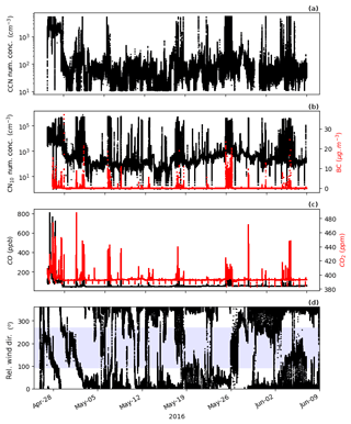
Figure A1 Time series showing that periods of CCN elevated above background values (typically less than 1000 cm⁻³) are associated with elevated concentrations of the other parameters, or wind directions in the exhaust sector. (a) CCN, (b) CN (left axis) and BC (right axis), (c) CO (left axis) and CO₂ (right axis), and (d) relative wind direction with the coloured region signifying those directions in which exhaust is expected.

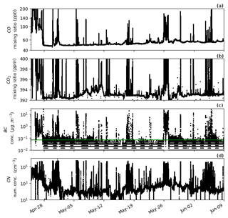
Figure A2 Time series (log scale) of CO, CO₂, BC and CN for 45 d of voyage IN2016_V03, which traversed from the ice edge to the Equator along the 170^∘ W meridian with a short personnel exchange port period in Wellington, New Zealand, on 26 May 2016. The green line in panel (c) represents the BC limit of 0.07 µg m⁻³ utilised. This dataset was utilised for the algorithm development as it exhibits influences from urban and background marine regions, by which differentiation from ship exhaust must be achieved.

Figure A3 As in Fig. A2 but with a linear y scale to reveal the baseline changes.

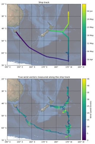
Figure A4 Voyage track of the data utilised in this voyage. Starting in Hobart, Australia, the voyage's primary goal was to perform ocean sampling along the 170^∘ W longitudinal line, with a brief personnel changeover in Wellington, New Zealand. This dataset was chosen as it contained clean marine background, as well as periods when it had increasing urban influence (as it travelled towards and arrived in Wellington), enabling fine tuning of the algorithm to only remove platform exhaust.

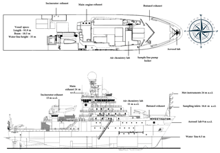
Figure A5 A schematic of the ship, with the two exhaust pipes marked – the main engine and the incinerator, along with the location of the main sampling inlets and met instruments on the foremast. Measurements of aerosol parameters (CN, BC and CCN) are carried out in the aerosol lab, while greenhouse gas measurements (CO and CO₂) are carried out in the air chemistry lab. The compass on the bird's eye view is oriented to show the wind direction as measured relative to the ship.

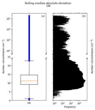
Figure A6 Distribution of the MADs calculated from rolling through CN number concentrations. (a) Box-and-whisker plot with quartiles drawn. Whiskers represent the quartiles ±1.5 times the interquartile range. (b) Histogram. Note the split axis, which changes from linear to logarithmic scaling.

Figure A7 As in Fig. A6 but for CO mixing ratios.

Figure A8 As in Fig. A6 but for CO₂ mixing ratios.

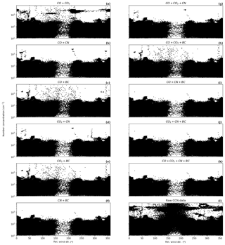
Figure A9 CCN data (log scale) with the different combinations of the algorithm applied separately: panels (a)–(f) show all two-parameter combinations, panels (g)–(j) show three-parameter combinations, panel (k) shows the filter using all four parameters and panel (l) shows unfiltered data for comparison. Note that the window filter is not applied to any of these plots.

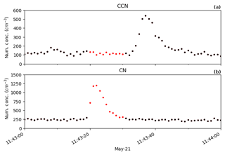
Figure A10 Time series of 1 min of time-synchronised aerosol data. Unfiltered data in red, with black markers showing exhaust-filtered data. The exhaust is clearly identified in the CN data but due to differences in instrument residence time, the exhaust signal shows up 10 s later in the CCN data, in this case, after the exhaust signal has ceased in the CN. While it is possible to align the underlying datasets based on an exhaust event, rather than by time, application of this method is unsuitable for this context because of the range of instrumentation where this exhaust product would be utilised (and thus the range of responses), and because the window filter applied after identification would result in a negligible improvement.

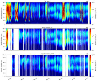
Figure A11 Aerosol size distributions measured using a GRIMM SMPS with M-DMA installed. Panel (a) shows all raw data recorded, while the wind-based filter and the exhaust algorithm are applied to the two subsequent graphs (b, c) respectively, removing periods identified as sampling exhaust.

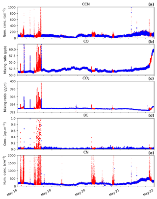
Figure A12 As in Fig. 2 but with the filtered dataset (blue) being the wind-based method. Unfiltered data are shown in red.

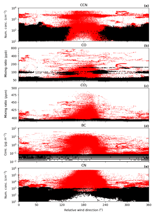
Figure A13 As in Fig. 2 but plotted against relative wind direction. Unfiltered data are shown in red, while data with the respective exhaust filter are shown in black.

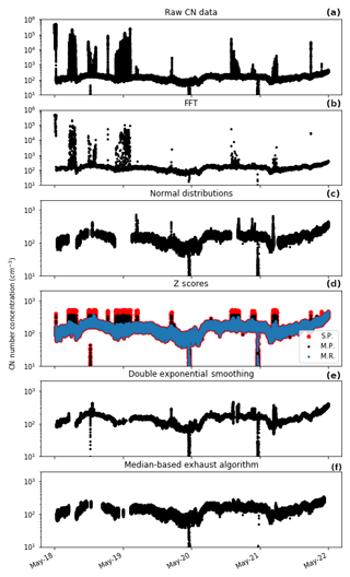
Figure A14 A subset of CN during the voyage with a range of outlier detection methods applied. (a) Raw CN data. (b) Fast Fourier transform (FFT). (c) Normal distribution filter. (d) Z scores: in red the standard method is applied to the whole population (S.P.); in black, the modified z score is applied to the whole population (M.P.); in blue, the modified z score is applied to a rolling window. (e) Double exponential smoothing. (f) The median-based method developed in this paper.