An adaptation of the CO₂ slicing technique for the Infrared Atmospheric Sounding Interferometer to obtain the height of tropospheric volcanic ash clouds

Ash clouds are a geographically far-reaching hazard associated with volcanic eruptions. To minimise the risk that these pose to aircraft and to limit disruption to the aviation industry, it is important to closely monitor the emission and atmospheric dispersion of these plumes. The altitude of the plume is an important consideration and is an essential input into many models of ash cloud propagation. CO₂ slicing is an established technique for obtaining the top height of aqueous clouds, and previous studies have demonstrated that there is potential for this method to be used for volcanic ash. In this study, the CO₂ slicing technique has been adapted for volcanic ash and applied to spectra obtained from the Infrared Atmospheric Sounding Interferometer (IASI). Simulated ash spectra are first used to select the most appropriate channels and then demonstrate that the technique has merit for determining the altitude of the ash. These results indicate a strong match between the true heights and CO₂ slicing output with a root mean square error (RMSE) of less than 800 m. Following this, the technique was applied to spectra obtained with IASI during the Eyjafjallajökull and Grímsvötn eruptions in 2010 and 2011 respectively, both of which emitted ash clouds into the troposphere, and which have been extensively studied with satellite imagery. The CO₂ slicing results were compared against those from an optimal estimation scheme, also developed for IASI, and a satellite-borne lidar is used for validation. The CO₂ slicing heights returned an RMSE value of 2.2 km when compared against the lidar. This is lower than the RMSE for the optimal estimation scheme (2.8 km). The CO₂ slicing technique is a relatively fast tool and the results suggest that this method could be used to get a first approximation of the ash cloud height, potentially for use for hazard mitigation, or as an input for other retrieval techniques or models of ash cloud propagation.

1 Introduction

Encounters of aircraft with volcanic ash have demonstrated that such occurrences can cause significant damage to the plane (Casadevall, 1994; Dunn and Wade, 1994; Pieri et al., 2002; Guffanti and Tupper, 2015). In extreme cases, these have resulted in engine failure (Miller and Casadevall, 2000; Chen and Zhao, 2015) and subsequently life-threatening circumstances. Ash clouds are closely monitored by the Volcanic Ash Advisory Centre (VAAC), who use a variety of data sources including information from volcano observatories and satellite data (Prata and Tupper, 2009; Thomas and Watson, 2010; Lechner et al., 2017). This allows informed decisions on the closure of airspace following an eruption, which can result in severe disruption and have significant financial implications. For example, the eruption of Eyjafjallajökull in 2010 resulted in the closure of a large portion of northern European airspace and subsequently the cancellation of 100 000 flights and a revenue loss of USD 1.7 billion (IATA Economic Breifing, 2010). Alongside these potential impacts to the aviation industry, volcanic ash is also a hazard to health (Horwell and Baxter, 2006; Horwell, 2007) and can cause considerable damage to infrastructure (Durant et al., 2010; Wilson et al., 2012, 2015).

Satellite remote sensing, particularly infrared instruments, has been widely used for monitoring the hazards presented by volcanic ash. This has included detection schemes which flag pixels that contain volcanic ash (e.g. Prata, 1989a, b; Ellrod et al., 2003; Pergola et al., 2004; Filizzola et al., 2007; Clarisse et al., 2010; Mackie and Watson, 2014; Taylor et al., 2015). Other methods have been developed to quantify parameters such as the mass, ash optical depth (AOD), effective radius and altitude of the ash cloud, usually relying on look-up tables or optimal estimation techniques (e.g. Wen and Rose, 1994; Yu et al., 2002; Watson et al., 2004; Corradini et al., 2008; Gangale et al., 2010; Francis et al., 2012; Grainger et al., 2013; Pavolonis et al., 2013).

Knowing the position of the ash cloud in three dimensions is critical for hazard mitigation. Plume height is a crucial part of this, and it is also a variable in models of ash cloud propagation (Mastin et al., 2009; Stohl et al., 2011; Bonadonna et al., 2012) such as HYSPLIT (Draxier and Hess, 1998; Stein et al., 2015) or NAME (Jones, 2004; Witham et al., 2012). A number of different methods have been used to obtain the height of volcanic ash clouds. These have included the use of ground-based and airborne instruments, as well as satellite techniques (Glaze et al., 1999), some of which are summarised in Table 1.

Patrick (2007)Sahetapy-Engel and Harris (2009)Webb et al. (2014)Bombrun et al. (2018)Lacasse et al. (2004)Arason et al. (2011)Petersen et al. (2012)Ansmann et al. (2010)Marenco et al. (2011)Winker et al. (2012)Vernier et al. (2013)Balis et al. (2016)Prata and Turner (1997)Zakšek et al. (2013)Holasek et al. (1996)Prata and Grant (2001b)Holasek et al. (1996)Eckhardt et al. (2008)Stohl et al. (2009)Kristiansen et al. (2010)Stohl et al. (2011)Pardini et al. (2017, 2018)Ventress et al. (2016)Zhu et al. (2017)

Table 1 A summary of some of the existing methods for determining the height of volcanic ash clouds. Summaries can be found in Oppenheimer (1998), Prata and Grant (2001a), Prata and Grant (2001b), and Zakšek et al. (2013).

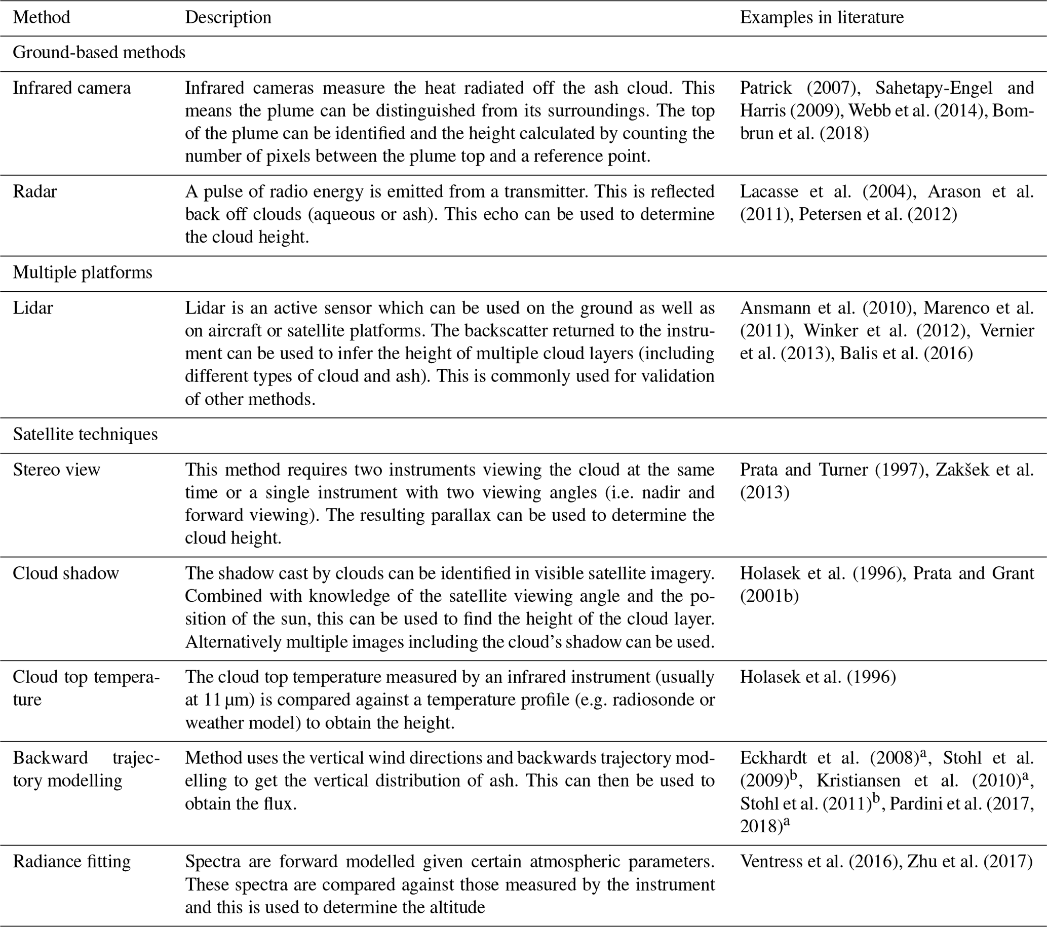
^a Example using SO₂ and not ash.
^b Example using hydrofluorocarbons and hydrochlorofluorocarbon.

Pangaud et al. (2009)Someya et al. (2016)Arriaga (2007)Smith and Platt (1978)Menzel et al. (1992)Richards (2006)Tupper et al. (2007)Menzel et al. (2008)Frey et al. (1999)Holz et al. (2006)Menzel et al. (1983)Wylie and Menzel (1989)

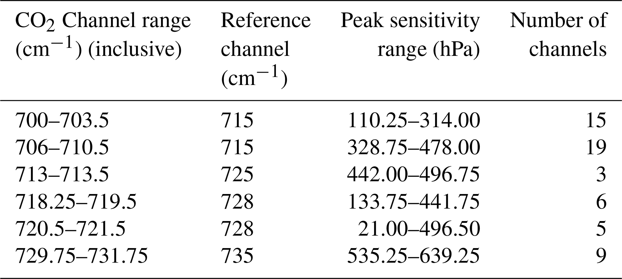
Table 2 A summary of some of the previous applications of the CO₂ slicing technique.

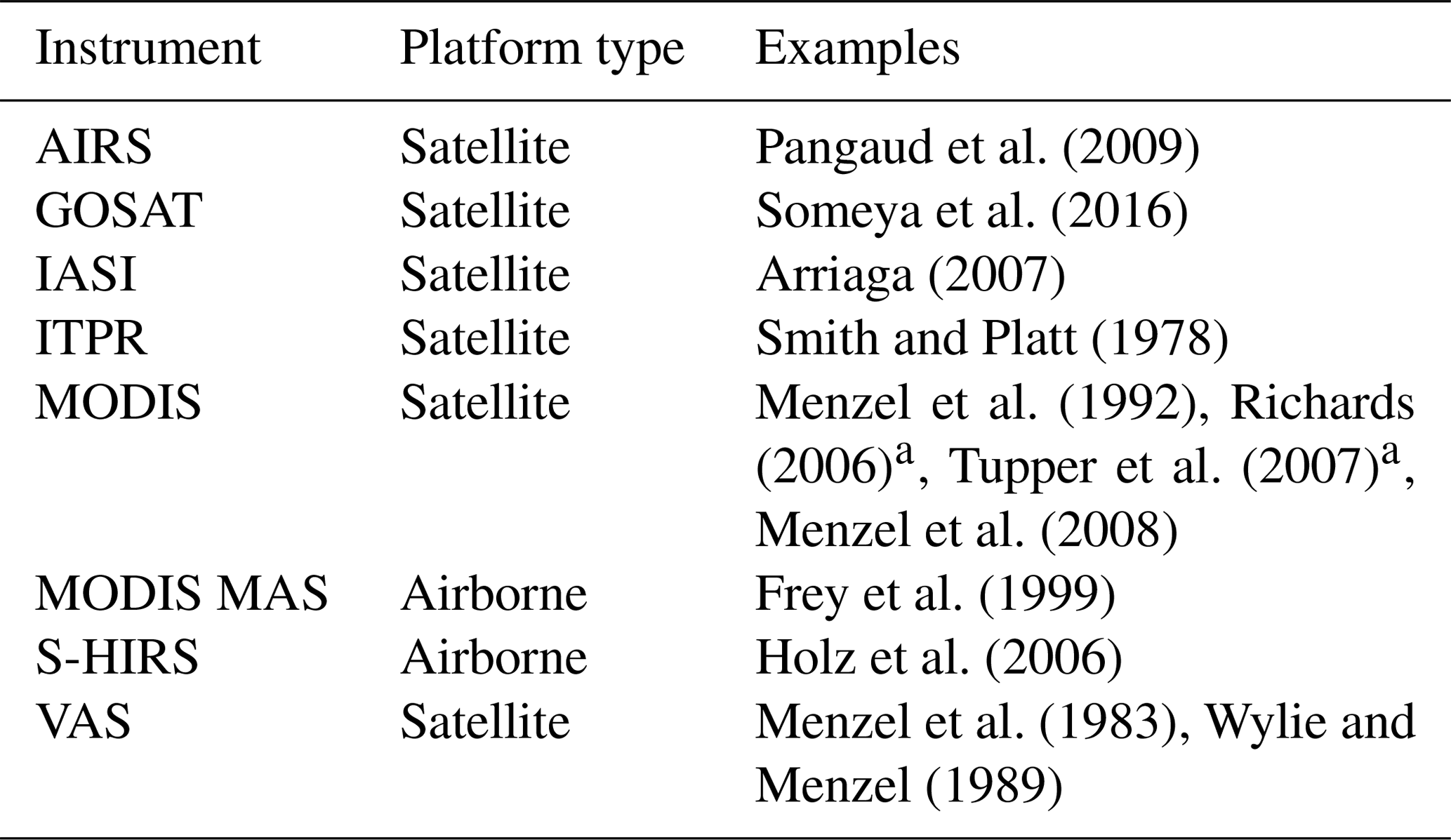
AIRS: Atmospheric Infrared Sounder.
GOSAT: the Greenhouse Gases Observing Satellite.
IASI: the Infrared Atmospheric Sounding Interferometer.
ITPR: Infrared Temperature Profile Radiometer.
MODIS: Moderate Resolution Imaging Spectroradiometer.
MODIS MAS: Moderate Resolution Imaging Spectroradiometer Airborne Simulator.
S-HIRS: Scanning High-Resolution Interferometer Sounder.
VAS: Visible IR spin-scan radiometer Atmospheric Sounder.
^a Studies applied to ash.

This problem is not unique to volcanic ash. Similar retrieval techniques exist to obtain the cloud height of aqueous clouds (i.e. water/ice clouds not associated with volcanic activity). One such method, known as the CO₂ slicing technique, described in more detail in Sect. 2, has been widely used to obtain the cloud top height and has been adapted for numerous instruments, as illustrated in Table 2. The method has been shown to have some potential when applied to volcanic ash using the Moderate Resolution Imaging Spectroradiometer (MODIS) (Richards, 2006; Tupper et al., 2007). In this study, the technique has been adapted for the Infrared Atmospheric Sounding Interferometer (IASI; see Sect. 3) and applied to volcanic ash. It was first applied to simulated ash spectra (Sect. 4) to select the most appropriate channels and to demonstrate that the method has promise when applied to volcanic ash. Following this it was applied to scenes containing volcanic ash from the Eyjafjallajökull and Grímsvötn eruptions (Sect. 5) where it was compared against an existing method for obtaining the height of volcanic ash and data from a satellite-borne lidar. The results indicate that this method could be applied to get a first approximation of the ash cloud height, which could then be used for hazard mitigation and as a parameter in other retrieval methods or ash models.

2 CO₂ slicing

The CO₂ slicing technique is an established method, developed for obtaining the cloud top height/pressure of aqueous cloud (Chahine, 1974; Smith and Platt, 1978; Menzel et al., 1983). Over the past four decades this tool has been adapted for different instruments, summarised in Table 2, including both airborne and satellite platforms. The technique uses a CO₂ absorption feature within the thermal infrared part of the electromagnetic spectrum between 665 and 750 cm⁻¹ (13.3 to 15 µm). Within this region, as wavenumber increases there is a general increase in the radiance observed. This is demonstrated in Fig. 1a, which shows the spectrum of a simulated clear atmosphere. This has been simulated with the fast radiative transfer model RTTOV (version 9; Saunders et al., 1998) and replicates what would be observed with IASI given specified atmospheric conditions. In this case a default atmospheric profile is used, without the addition of cloud, volcanic ash, or any trace gases or aerosols above background levels.

In the Earth's troposphere where temperature is decreasing with height, the radiances measured by the instrument are proportional to the transparency of the atmosphere for each channel (Holz et al., 2006). Subsequently, within the CO₂ absorption band, as wavenumber and the radiance measured both increase, the channels are becoming increasingly transparent (with some fluctuations). As such, the spectrum of a high-altitude cloud will begin to deviate from the clear spectrum at a lower wavenumber than a lower-altitude cloud. This is illustrated in Fig. 1a, which shows the spectra of three ash clouds of varying heights. Effectively, until the point where the clear and ash/cloudy spectra diverge, the instrument is recording clear radiances. This concept has been used to identify channels whose cloud-free radiances can be assimilated into numerical weather prediction models rather than filtering out these pixels entirely (e.g. McNally and Watts, 2003).

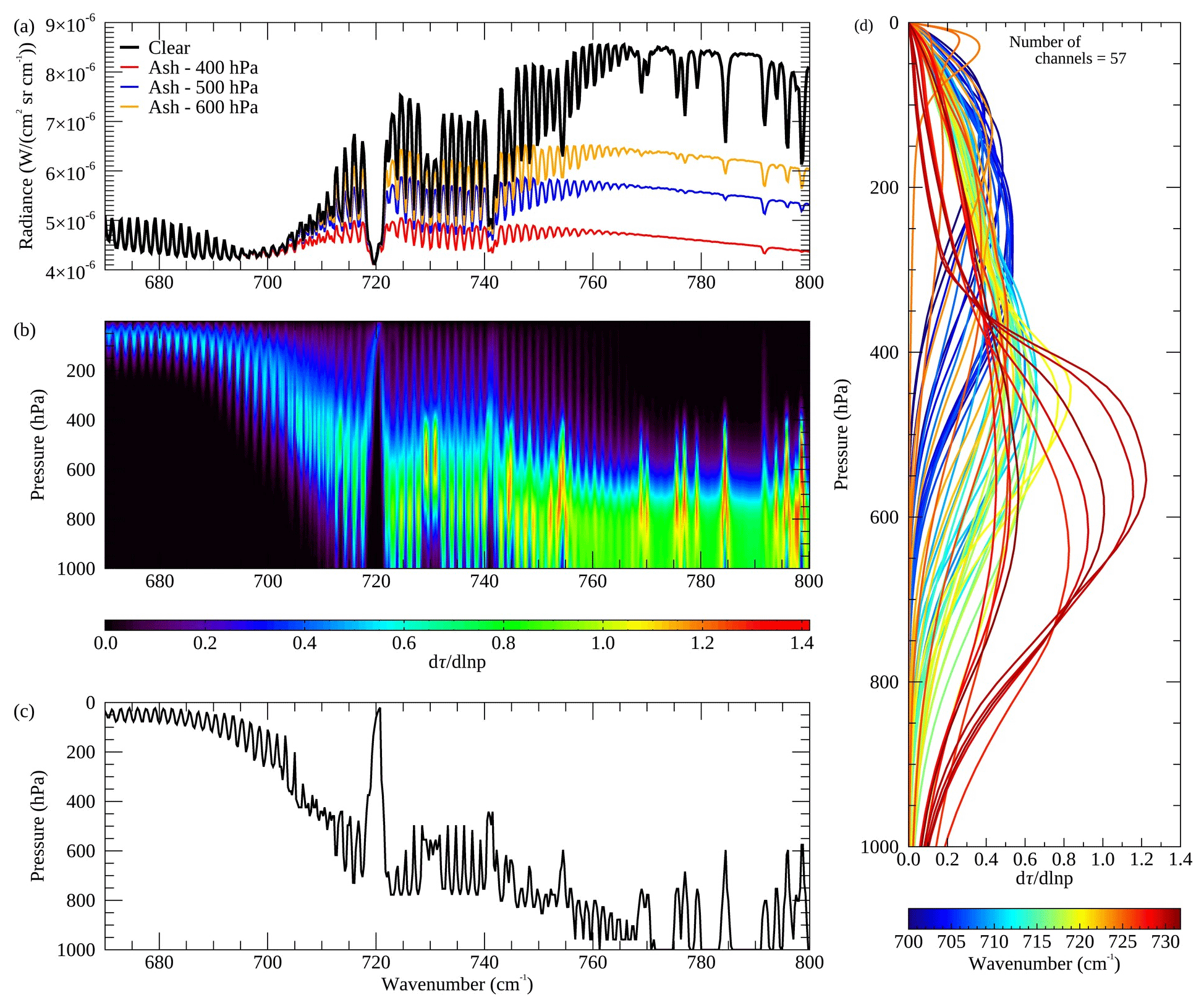
Figure 1 (a) Simulated spectra for a clear atmosphere (i.e. one without cloud or ash) and three ash clouds at different pressure levels: 400, 500 and 600 hPa. (b) The change in atmospheric transmittance with log pressure (dτ∕dln p). This is indicative of which part of the atmosphere each channel is sensitive to. This sensitivity is shown to shift from higher up in the atmosphere to the lower parts of the atmosphere as wavenumber increases. (c) The peak sensitivity for each channel. (d) The weighting function (dτ∕dln p) for the 57 channels used in this CO₂ slicing study.

The changing sensitivity of each of the channels to the atmospheric profile is better demonstrated in Fig. 1b and c. This shows the derivative of atmospheric transmittance with log pressure (dτ∕dln p) and the peak of this value respectively. This is a measure of each channel's sensitivity to each level of the atmosphere and demonstrates that this shifts from the upper atmosphere at lower wavenumbers towards the surface at higher wavenumbers.

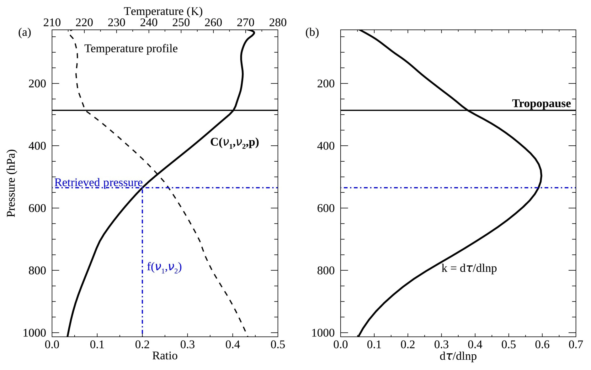
Figure 2 (a) An example of the cloud pressure function calculated using Eq. (2). This is strongly linked to the atmospheric temperature profile (dashed black line). The value obtained with Eq. (1) is compared against the cloud pressure function, and where these intersect is taken as the cloud pressure solution for that channel. In this example ν₁ and ν₂ are at 715 and 725 cm⁻¹ respectively. (b) The corresponding weighting functions (dτ∕dln p) which illustrate the changing sensitivity to the atmosphere. This is used to obtain a weighted average from multiple channel solutions.

As the channels are sensitive to different parts of the atmosphere, it is possible to use this to estimate the height of the cloud (aqueous or in principle ash). To do this using the CO₂ slicing method, the ratio (f, Eq. 1) of the difference in cloudy and clear radiances (L_obs and L_clr respectively) for two channels (ν₁and ν₂) within or close to the CO₂ absorption band is compared against a cloud pressure function (C, Eq. 2):

$$\begin{array}{}\text{(1)}& {\displaystyle }f({\mathit{\nu }}_{\mathrm{1}},{\mathit{\nu }}_{\mathrm{2}})={\displaystyle \frac{L_{\mathrm{obs}}\left({\mathit{\nu }}_{\mathrm{1}}\right)-L_{\mathrm{clr}}\left({\mathit{\nu }}_{\mathrm{1}}\right)}{L_{\mathrm{obs}}\left({\mathit{\nu }}_{\mathrm{2}}\right)-L_{\mathrm{clr}}\left({\mathit{\nu }}_{\mathrm{2}}\right)}},\text{(2)}& {\displaystyle }C({\mathit{\nu }}_{\mathrm{1}},{\mathit{\nu }}_{\mathrm{2}},p)={\displaystyle \frac{N{\mathit{\epsilon }}_{\mathrm{1}}{\int }_{p_{\mathrm{s}}}^{p_{\mathrm{c}}}\mathit{\tau }({\mathit{\nu }}_{\mathrm{1}},p)\frac{\mathrm{d}B[{\mathit{\nu }}_{\mathrm{1}},T(p\left)\right]}{\mathrm{d}p}\mathrm{d}p}{N{\mathit{\epsilon }}_{\mathrm{2}}{\int }_{p_{\mathrm{s}}}^{p_{\mathrm{c}}}\mathit{\tau }({\mathit{\nu }}_{\mathrm{2}},p)\frac{\mathrm{d}B[{\mathit{\nu }}_{\mathrm{2}},T(p\left)\right]}{\mathrm{d}p}\mathrm{d}p}},\end{array}$$

where τ is the atmospheric transmittance at channel ν of the layer between the pressure level p and the instrument (top of the atmosphere); B is the Planck radiance which is channel and temperature (and therefore pressure) dependent; p_c and p_s are the cloud and surface pressure respectively; and Nε is the effective emissivity (sometimes referred to as the effective cloud amount), a product of the cloud fraction (N) and cloud emissivity (ε). Equation (1) is compared against Eq. (2) and where the two functions intersect is taken as the cloud top pressure. A demonstration of this is shown in Fig. 2a. Following this the effective emissivity can be computed using a channel which falls within an atmospheric window (w; usually one close to the CO₂ absorption band):

$$\begin{array}{}\text{(3)}& N\mathit{\epsilon }={\displaystyle \frac{L_{\mathrm{obs}}\left(w\right)-L_{\mathrm{clr}}\left(w\right)}{B[w,T(p_{\mathrm{c}}\left)\right]-L_{\mathrm{clr}}\left(w\right)}}.\end{array}$$

In most applications of the CO₂ slicing technique, multiple channel pairs are used, resulting in different height solutions. In many studies, channel pairs are not considered if L_obs(ν)−L_clr(ν) for either the CO₂ (ν₁) or reference (ν₂) channels used falls within the noise of the instrument at that channel (e.g. Menzel et al., 1992). The solution may also be rejected if the effective emissivity computed using Eq. (3) is not between 0 and 1.05 (e.g. Arriaga, 2007). If multiple solutions remain, then a number of different techniques can be employed to obtain a final value. This includes a top-down approach where the solution of the most opaque channel is accepted if it is within an expected height range, and if not the next most opaque channel is considered. This is repeated until an appropriate height value is obtained (Menzel et al., 2008). Alternatively, the height and cloud fraction which best satisfies the radiative transfer equation for all the channels used is accepted as the final cloud pressure/height (e.g. Menzel et al., 1983, 1992). If all of the channel pairs are considered inappropriate, for example, if L_obs(ν)−L_clr(ν) is within the noise of the instrument for all the channels used, then many methods assume that cloud is opaque and compare the brightness temperature measured by the instrument at 11 µm to an atmospheric temperature profile to obtain an alternative cloud height (e.g. Menzel et al., 1983, 1992; Zhang and Menzel, 2002; Menzel et al., 2008).

The issue of multiple solutions is further complicated for hyperspectral instruments as these can have hundreds of channels within the CO₂ absorption band. Some methods apply a weighting function based on each channel's sensitivity to the atmosphere (e.g Smith and Frey, 1990). However, to avoid a high computational cost, often there needs to be some prior consideration of the most appropriate channels. This has included exploring large datasets with known cloud top heights to select the most appropriate channels (e.g. Arriaga, 2007). Other approaches include the creation of synthetic channels by averaging the radiances of channels sensitive to the same portion of the atmosphere (Someya et al., 2016) or CO₂ sorting which looks for the point where the clear and cloudy spectra deviate, which is the first point where the instrument can see the cloud layer (Holz et al., 2006).

The CO₂ slicing method makes a number of assumptions: (1) the cloud is infinitesimally thin; (2) in cases where there are multiple layers of cloud, the lower-level clouds are ignored; (3) the two channels used in Eq. (1) are sufficiently close that the difference in emissivity between them is negligible – this is particularly important to consider when the channel pairs are selected. Multiple cloud layers have previously been identified as a source of error in the CO₂ slicing retrieval, with the extent of this being affected by the channels used and the height of the underlying layers (Menzel et al., 1992). For example, an opaque cloud close to the surface is unlikely to affect the height retrieval of a cirrus cloud when using channels which are not sensitive to radiation from the lower troposphere. In contrast, an opaque cloud in the middle of the troposphere might lead to the underestimation of the cloud top height of a higher cirrus layer (Menzel et al., 1992). The effect of surface emissivity is expected to be minimal as channels within the CO₂ absorption band have weighting functions that peak above the surface, as shown in Fig. 1d.

An additional consideration has to be made when applying the CO₂ slicing method to volcanic ash. The height that a volcanic ash cloud reaches is largely dependent on the force of the eruption and the atmospheric conditions (Sparks et al., 1997), and so this can vary widely. Large explosive eruptions can generate columns which enter the stratosphere, which can then potentially affect climate (Robock, 2000). The cloud pressure function generated using Eq. (2) is temperature dependent. Within the troposphere, the temperature decreases with height; however, in the stratosphere the temperature beings to climb again. This leads to a reversal in the cloud pressure function, which in some cases can result in multiple solutions: one in the troposphere and one in the stratosphere. Consequently, some prior information is required to determine whether the plume is within the troposphere and therefore if the CO₂ slicing technique is appropriate. This might include observations made on the ground or by pilots. The CO₂ slicing technique has previously only been used to determine the height of aqueous clouds in the troposphere, and so in this study only the tropospheric solution is accepted.

3 The Infrared Atmospheric Sounding Interferometer

The Infrared Atmospheric Sounding Interferometer (IASI) is an instrument on board three meteorological satellites, Metop A, B and C, launched in 2006, 2012 and 2018 respectively. Each instrument orbits the Earth twice a day. The instrument scans have a swath width of 2200 km and consist of groups of four circular pixels which have a diameter of 12 km at nadir (Clerbaux et al., 2009). The instruments measure across the infrared between 645 and 2760 cm⁻¹ (3.62 to 15.5 µm) with a high spectral resolution of 0.5 cm⁻¹ (Blumstein et al., 2004).

The instrument has previously been used to analyse volcanic plumes of SO₂ (e.g. Clarisse et al., 2008, 2012, 2014; Walker et al., 2012; Carboni et al., 2012, 2016; Taylor et al., 2018) and ash (e.g. Clarisse et al., 2010; Maes et al., 2016; Ventress et al., 2016) from a number of different eruptions. Previous methods for determining the height of the plume with spectra measured by IASI use the optimal estimation method (Maes et al., 2016; Ventress et al., 2016). The CO₂ slicing method has previously been applied to IASI spectra to obtain the cloud top height of aqueous cloud (Arriaga, 2007). The values obtained for the cloud pressure and emissivity are often assimilated in numerical weather prediction models (Guidard et al., 2011; Lavanant et al., 2011). The different adaptations of the CO₂ slicing technique for IASI use different numbers and combinations of channels and can therefore give different results (Lavanant et al., 2011). In this study, channels are selected based on the technique's performance when applied to simulated ash spectra.

4 Application to simulated data

4.1 Channel selection

IASI has over 300 channels which fall within the CO₂ absorption band, and so to ensure computational efficiency an appropriate subset of these channels must be selected. To do this the CO₂ slicing technique was first applied to 384 simulated ash spectra. These are ideal test cases, which do not include other aerosols or aqueous cloud. These spectra include six different atmospheres: high latitude, mid-latitude day and night, tropical daytime, and polar summer and winter (including atmospheric profiles created for the Michelson Interferometer for Passive Atmospheric Sounding, MIPAS; Remedios et al., 2007). The spectra were modelled using the refractive indices of samples of volcanic ash from the Eyjafjallajökull eruption in 2010 (Peters, 2010): the main eruption considered in this study. In the future different refractive indices could be used, such as those in Prata et al. (2019). A range of ash properties were explored: cloud heights between 200 and 900 hPa (going slightly above the tropopause), ash effective radius between 5 and 10 µm, and ash optical depths between 5 and 15 (referenced at 550 nm). Typically, the effective radius is less than 8 µm for very fine ash (such as in a distal plume) and between 8 and 64 µm for fine ash (Marzano et al., 2018). The range of ash optical depths is highly variable. Ventress et al. (2016) and Balis et al. (2016) recorded ash optical depths of less than 1.2 from dispersed plumes from Eyjafjallajökull in 2010; however much higher values can be expected closer to the volcano or following large explosive eruptions. The effective radius and AOD explored here for the channel selection are in the upper range and above what might be expected: values which may only be true close to the volcanic vent. The spectrum of an optically thin plume is more difficult to differentiate from a clear spectrum, commonly leading to the signal (I_obs(v)−I_clr(v)) being within the instrument noise and subsequently resulting in no retrieval. A decision was made to select the channels used using idealised optically thick cases, which may only be true close to the vent, for which the plume should be evident in the majority of the CO₂ channels. The selected channels are tested on a wider range of AODs and effective radius, including smaller values that are more representative of a disperse plume (in Sect. 4.2).

The CO₂ slicing method was first applied using every channel combination between 660 and 800 cm⁻¹, where the reference channel (ν₂) wavenumber is greater than the CO₂ channel (ν₁) wavenumber. In this way, the reference channel is generally more sensitive to a lower part of the atmosphere than the CO₂ channel. As with existing studies only tropospheric solutions were accepted, and, in cases where the curve of the cloud pressure function resulted in multiple solutions, the solution with the greater weight (in this case the weighting function is defined as $k=\mathrm{d}\mathit{\tau }[{\mathit{\nu }}_{\mathrm{1}},p]/\mathrm{d}\ln p)$ was accepted. The output from each channel pair was only accepted if it met three quality control criteria: (1) L_obs(ν₁)−L_clrν(₁) must be greater than the noise of the instrument at channel ν₁ (CO₂ channel; within the CO₂ absorption band the noise of the IASI instruments is between $\mathrm{2.55}\times {\mathrm{10}}^{-\mathrm{8}}$ and $\mathrm{3.77}\times {\mathrm{10}}^{-\mathrm{8}}$ $\mathrm{W}({\mathrm{cm}}^{\mathrm{2}}\mathrm{sr}{\mathrm{cm}}^{-\mathrm{1}}{)}^{-\mathrm{1}}$); (2) similarly, L_obs(ν₂)−L_clr(ν₂) must be greater than the noise of the instrument at ν₂ (reference channel); (3) the solution to Eq. (3) must fall between 0 and 1.05 (following Arriaga, 2007).

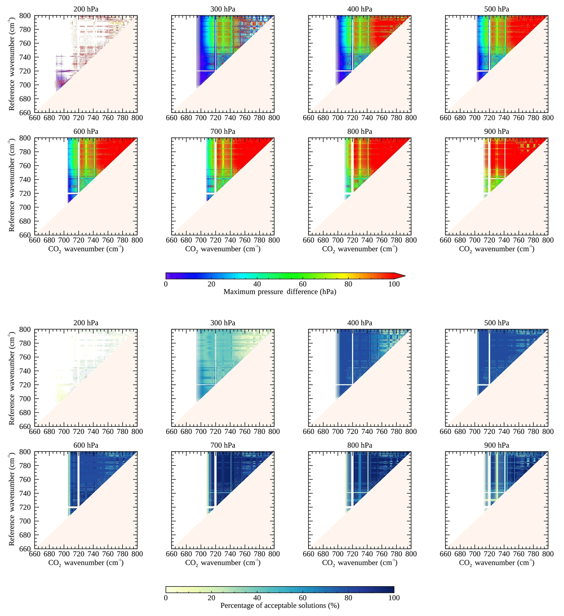
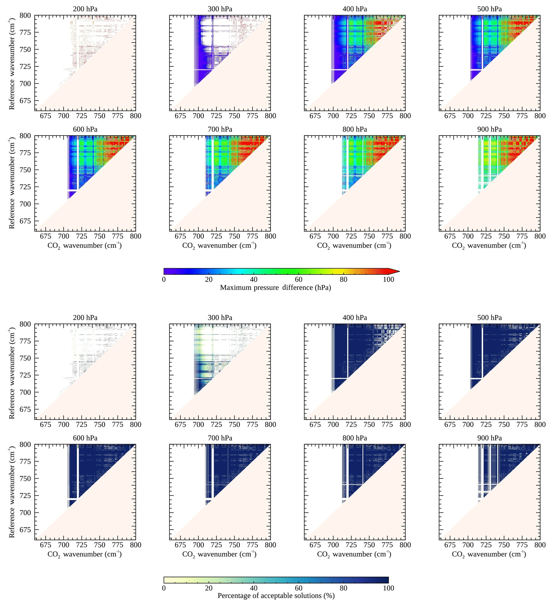
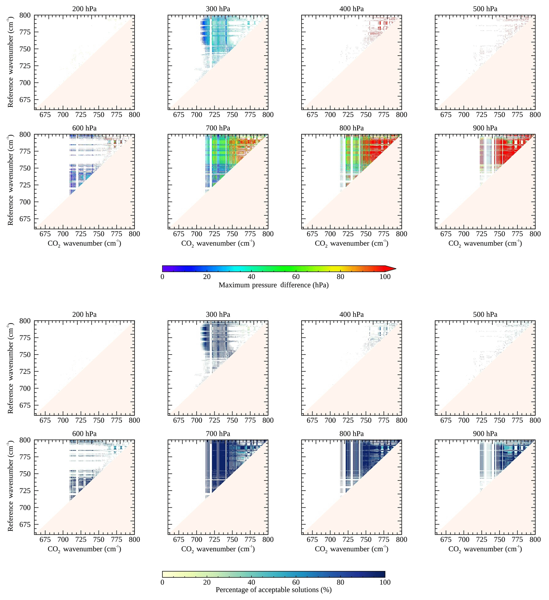
Figure 3 CO₂ slicing results for simulated ash spectra. The technique has been applied for each channel pair between 660 and 800 cm⁻¹. A total of 384 spectra were used which includes six different atmospheres. It also includes ash optical depths between 5 and 15, effective radius ranging between 5 and 10 µm, and pressures between 200 and 900 hPa. The first two rows of the plot show the maximum difference between the known (simulated) pressure and the pressure retrieved with the CO₂ slicing algorithm. This is divided into each pressure level. The last two rows show the percentage of successful retrievals. This is again divided into the eight different pressure levels. In these plots the colour white indicates where no successful retrieval has been made and off-white indicates channel combinations not explored in this study.

The results are shown in Fig. 3. The top two rows show the maximum pressure difference between the true (simulated) and CO₂ slicing retrieved values divided into each pressure level. In total there are 48 spectra for each pressure level with these incorporating the different atmospheric profiles and ash properties. The lower two rows of Fig. 3 show the percentage of accepted retrievals. This refers to where there was an intersection between the two functions shown in Eqs. (1) and (2) and where the value retrieved meets all three quality control conditions. This is also grouped into the eight pressure levels. The equivalent plots for the six individual atmospheres can be seen in Figs. A1–A6 in the Appendix. Potentially, the method used in this study to select the most appropriate channels could be performed for the different atmospheres to select channels which might be more suited to specific climatologies.

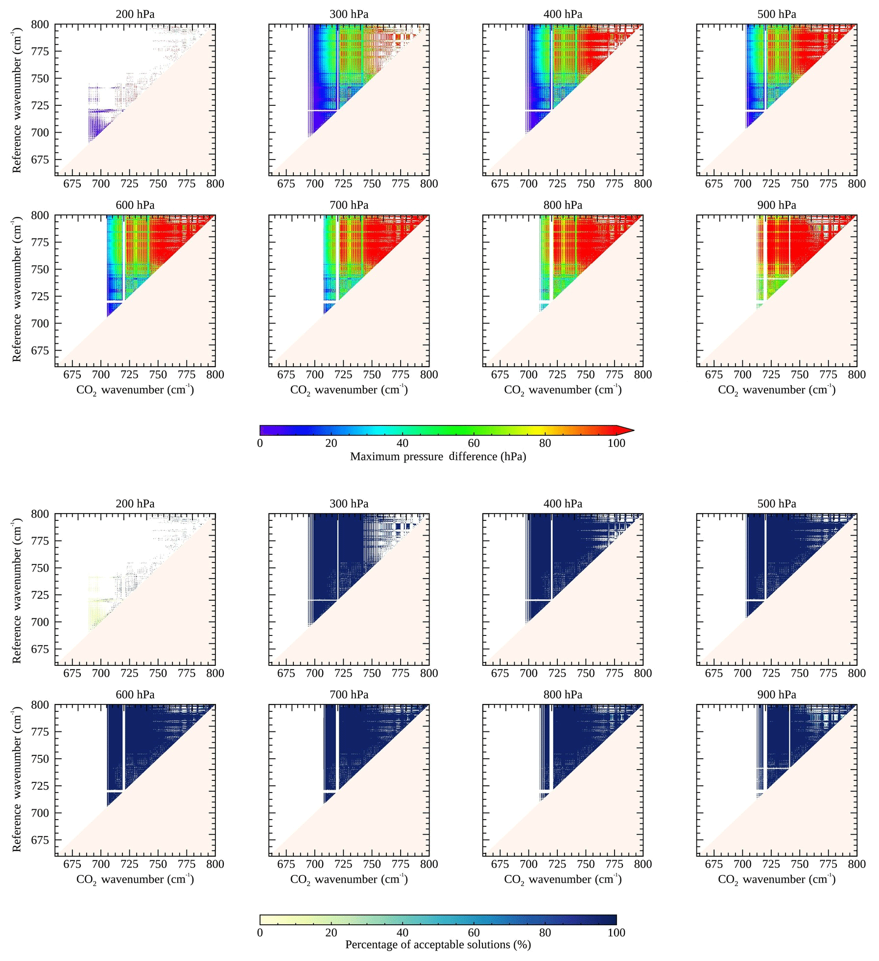
Figure 4 CO₂ slicing results for RTTOV simulated ash spectra. The plots show the maximum difference between the true (simulated) pressure and the pressure obtained with the CO₂ slicing algorithm. The results are split into three pressure levels: (a) high cloud (300–400 hPa), (b) mid-level cloud (500–600 hPa) and (c) low-level cloud (700–800 hPa). Note that, in this plot, results for 200 and 900 hPa are excluded. Results are only included where the maximum difference is less than 75 hPa and the percentage of successful retrievals is greater than 50 %. This was used to inform the choice of channels for the final CO₂ slicing algorithm.

Figure 3 demonstrates that the best-performing channel pairs vary depending on the height of the plume. For plumes at lower pressures, the maximum pressure difference between the simulated and retrieved pressures is smaller at lower CO₂ wavenumbers. For example, for the plumes simulated at 300 hPa, the maximum pressure difference was lowest (less than 20 hPa) for CO₂ channels between 700 and 710 cm⁻¹. As the pressure of the ash layer is increased, values are no longer obtained at smaller wavenumbers. For example, for a plume at 500 hPa, solutions are no longer obtained for CO₂ channels which are less than 700 cm⁻¹: the maximum pressure difference between the true and retrieved values is now smaller for slightly higher wavenumbers. For a plume at 800 hPa the maximum pressure difference is lowest (less than 60 hPa) for CO₂ channels between 715 and 720 cm⁻¹. This observation reflects what is shown in Fig. 1b and c: that the channel's peak sensitivity shifts from higher in the atmosphere at lower wavenumbers to close to the surface as higher wavenumbers effecting the best-performing channel combinations. Notably, at 200 hPa there are far fewer channels which pass the quality control conditions, and where a retrieval is possible, there is a large difference between the true and retrieved pressure. It is also possible to identify an increased error closer to the surface. Previous studies have acknowledged that the CO₂ slicing tool is less successful at pressures greater than 700 hPa (Menzel et al., 2008) because approaching the surface there are fewer channels with a distinction between the clear and cloudy spectra, often leading to L_obs(v)−L_clr(v) being within the range of the instrument's noise and therefore the channels being excluded. Another observation that can be made from Fig. 3 is that channels below 700 cm⁻¹ often have a low percentage of accepted retrievals. These channels are shown in Fig. 1b and c to be sensitive to the heights above the tropopause. This may also be the reason for few accepted retrievals at 720 cm⁻¹. Additionally, for channels greater than 750 cm⁻¹, which are no longer in the CO₂ absorption band, the difference between the true and retrieved pressure is usually greater than 100 hPa.

Figure 4 shows a similar plot between 700 and 750 cm⁻¹. In this case, the spectra were also grouped into three categories: high cloud (300–400 hPa), mid-level cloud (500–600 hPa) and low-level cloud (700–800 hPa). Note that the simulated spectra at 200 and 900 hPa have been excluded. Also, the maximum pressure difference is only shown where it is less than 75 hPa and where the percentage of successful retrievals is greater than 50 %. This plot has been used to manually select the most appropriate set of channels. The best selection of channel pairs will be representative of the entire atmosphere (channels which peak at different heights should be selected, Fig. 1c), while minimising the difference between the simulated and retrieved pressures and maximising the acceptance rate (Fig. 4). Another consideration is the assumption that the change in emissivity between the channel pairs is negligible. The emissivity ratio for a sample of ash from the Eyjafjallajökull eruption (the main eruption considered in this study) for all channel combinations in the 680 and 800 cm⁻¹ range is shown in Fig. 5. For this assumption to hold true, the emissivity ratio should be as close to 1 as possible. This is usually the case for channels which are close together. Given these criteria, appropriate channel ranges have been selected. These channel ranges and the reference channels are shown in Table 3. The weighting functions for the selected channels are shown in Fig. 1d.

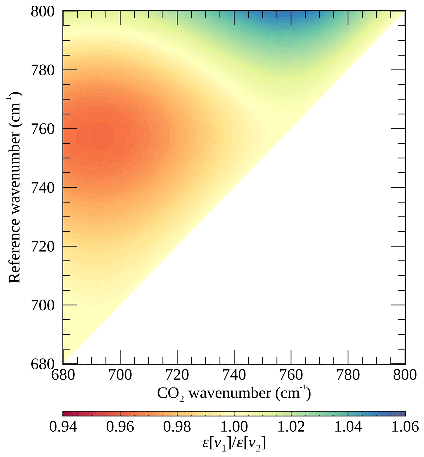
Figure 5 Emissivity ratio for channels between 680 and 800 cm⁻¹. The ash sample was from the Eyjafjallajökull eruption in 2010. The assumption that the emissivity does not vary significantly for the pair of channels used for the CO₂ slicing is important. For this to hold true, ideally the emissivity ratio should be close to 1.

Table 3 The channel ranges selected for the final application of the CO₂ slicing technique. In total 57 channels are used. Following Arriaga (2007), 900.50 cm⁻¹ is used as the window channel used to calculate the effective emissivity.

4.2 Simulation results

Following the selection of channels, the final pressure values (P) were computed by taking a weighted average of the results:

$$\begin{array}{}\text{(4)}& P={\displaystyle \frac{\sum p_{\mathrm{c}}\left(\mathit{\nu }\right)k^{\mathrm{2}}\left(\mathit{\nu }\right)}{\sum k^{\mathrm{2}}\left(\mathit{\nu }\right)}},\end{array}$$

where p_c is the pressure retrieved for channels ν, and k refers to the weighting function based on the derivative of atmospheric transmittance computed for each pressure level with RTTOV with respect to the log of atmospheric pressure ($\mathrm{d}\mathit{\tau }[\mathit{\nu },p]/\mathrm{d}\ln p$). On this occasion, the retrieval was applied to 1344 simulated ash spectra, including those with lower ash optical depths (ranging from 0.5 to 15) and smaller effective radius (ranging from 1 to 10 µm). This includes spectra representative of thinner ash clouds which were not considered during the channel selection.

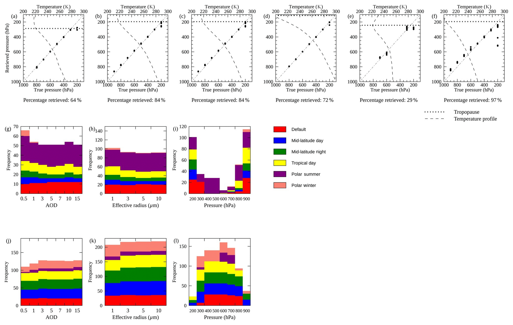
Figure 6 Final CO₂ slicing pressure results for RTTOV simulated ash spectra (a total of 224 spectra per atmosphere). Panels (a)–(f) show the true (simulated) pressure plotted against the CO₂ slicing retrieved value for the six different atmospheres. (a) RTTOV default atmosphere (high latitude), (b) mid-latitude day, (c) mid-latitude night, (d) tropical day, (e) polar summer, and (f) polar winter. In this case, the simulated spectra include the following ash properties: ash optical depth ranging between 0.5 and 15, ash effective radius ranging between 1 and 10 µm, and pressure values between 200 and 900 hPa. Below each plot is a value indicating the percentage of successful retrievals (where a height value can be obtained and all quality control conditions have been met). (g) The frequency of ash optical depths for which the CO₂ slicing technique was unable to return a height value. (h) Same as (g) for the effective radius. (i) Same as (g) for the ash cloud pressure. (j) The frequency of ash optical depths for which the difference between the simulation and CO₂ slicing height is less than 0.5 km. (k) The same as (j) for effective radius. (l) The same as (j) for ash cloud pressure. Related statistics can be seen in Table 4. The equivalent plot, where the quality control was not applied, has been included in the Appendix (Fig. A7).

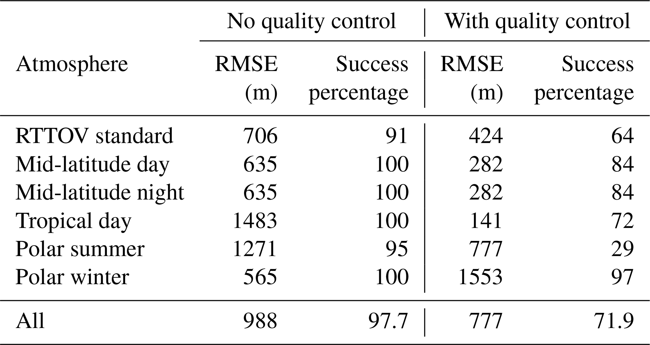
The results are displayed in Fig. 6a–f, which plot the true (simulated) pressures against the final weighted pressures obtained with the CO₂ slicing technique. The different atmospheres are displayed separately and the percentage of accepted retrievals are indicated below each plot. Table 4 reports the root mean square error (RMSE) for each atmosphere. Overall, the CO₂ slicing method returned values for 72 % of the simulated spectra, with an RMSE of 777 m. These results suggest that the technique does have merit for obtaining the height of ash clouds.

Figure 6g–i give some indication of where and why the retrieval was unsuccessful. Figure 6g–h show there are slightly more failed cases for ash spectra with the lowest optical depth (0.5) and effective radius (1 µm). These low values are representative of thinner ash clouds whose spectra are more similar to clear atmospheric spectra. Subsequently, these cases are likely to fail the signal-to-noise quality control tests (Menzel et al., 1992, 2008). For example, an ash cloud at 500 hPa only has 7 channels which pass the L_obs(ν₁)−L_clr(ν₁) quality control condition when the ash optical depth is 0.1. However, the number of channels passing this criterion increases to 38 at an ash optical depth of 2.3. This observation is supported by Fig. 6j–k, which show the number of cases where the difference between the simulated and retrieved pressure is less than 0.5 km, which is slightly lower for a smaller effective radius and ash optical depth.

The majority of failed cases are shown to be at the pressure extremes (Fig. 6i). Similarly, Fig. 6l indicates that there are fewer cases where the pressure difference between the simulated and retrieved pressures is less than 0.5 km at these pressures. Close to the surface this can again be attributed to less distinction between the clear and ashy spectra (Menzel et al., 2008). For example, for the RTTOV default atmosphere, an ash plume at 900 hPa fails the signal-to-noise condition for all the channels used regardless of the optical depth and effective radius of the simulation. The lowest simulation pressure (200 hPa) is close to or above the tropopause for all six atmospheres, and for this example the CO₂ slicing method was allowed to retrieve up to the height of the reversal of the temperature profile (which is slightly above the tropopause). At these heights, the temperature gradient (dT∕dp) is relatively stable, causing a similar effect in the cloud pressure function (best illustrated in Fig. 2) and subsequently a greater number of unsuccessful retrievals: the CO₂ slicing technique has previously been shown to perform poorly in isothermal regions of the atmosphere (Richards et al., 2006). This may also be the reason for the poor performance of the CO₂ slicing technique when applied to the polar summer atmosphere for which the technique only retrieved values for 29 % of cases.

The RMSE and the percentage of accepted retrievals for the CO₂ slicing technique, without the quality control criteria applied, are shown in Table 4. Figure A7 shows the equivalent plot to Fig. 6 without the quality control. The addition of the quality control compromises the number of successful retrievals for an overall reduction in the RMSE. Overall, the reduction is around 200 m but in individual cases up to 1.4 km (e.g. tropical atmosphere). Figure A7 indicates that the addition of the quality control is particularly advantageous for lower-level ash layers which without the quality control are often overestimated. Overall, the results show that this adaptation of the CO₂ slicing technique has promise for obtaining the height of volcanic ash clouds within the troposphere, although its use is limited in cases of low-level or thin clouds or where there is a steep temperature gradient.

Table 4 Summary of the percentage of accepted retrievals and the RMSE describing the difference between the true (simulated) and retrieved values.

5 Application to scenes containing volcanic ash

The CO₂ slicing method has been applied to scenes containing ash from the Eyjafjallajökull (63.63^∘ N, 19.63^∘ W; 1651 m) and Grímsvötn (64.42^∘ N, 17.33^∘ W; 1725 m) eruptions in 2010 and 2011 respectively. The plumes from both eruptions were closely monitored using a variety of instrumentation which included ground-based remote sensing, airborne measurements and the use of satellite products (e.g. Gudmundsson et al., 2010; Weber et al., 2012). The ash and gas clouds from these eruptions have since been extensively studied (e.g. Kerminen et al., 2011; Tesche et al., 2012; Flemming and Inness, 2013; Cooke et al., 2014; Ventress et al., 2016). They are commonly used to demonstrate the utility of new remote sensing developments (e.g. Mackie and Watson, 2014; Taylor et al., 2015; Ventress et al., 2016; Western et al., 2017) and similarly are often used in modelling research (Matthias et al., 2012; Webster et al., 2012; Moxnes et al., 2014; Wilkins et al., 2016). This makes them the ideal first candidates for the CO₂ slicing technique. Another reason for choosing these eruptions is that, in both cases, the ash clouds were confined to the troposphere, making them an appropriate target for the CO₂ slicing technique.

In this application of the retrieval, it has only been applied to pixels which are flagged as containing volcanic ash by a linear ash retrieval developed for IASI (Ventress et al., 2016; Sears et al., 2013: following the method developed for SO₂ by Walker et al., 2012). This method compares each IASI spectra against a covariance matrix formed from pixels which contain no volcanic ash, thereby representing the spectral variability associated with interfering gas species or clouds, and also the instrument noise. A least-squares fit is performed for three ash altitudes (400, 600 and 800 hPa) to retrieve a value for ash optical depth. A pixel is then flagged if it exceeds a threshold at any height. As SO₂ can, with caution, be used as a proxy for volcanic ash (Carn et al., 2009; Thomas and Prata, 2011), the retrieval has also been run for pixels flagged for SO₂ using the same approach (Walker et al., 2011, 2012; Carboni et al., 2012, 2016). For the CO₂ slicing, values for L_clr were obtained using the radiative transfer model RTTOV using the European Centre for Medium-Range Weather Forecasts (ECMWF) atmospheric profile as an input and using the default ocean emissivity within RTTOV. The effect of surface emissivity is thought to be minimal as for the channels used the weighting functions peak above the surface (Fig. 1d). The temperature and humidity profiles needed to calculate the Planck radiance and τ were acquired from ECMWF. The closest ECMWF profile to each individual IASI pixel was used. RTTOV was used to compute the transmittance values. Another point to note is that, in Sect. 4, the maximum height that could be retrieved was defined as the height at which the temperature profile inverts and has a positive gradient. This is slightly above the tropopause, which is defined by the World Meteorological Organisation (WMO) as the point at which the lapse rate is less than 2 ${}^{\circ }\mathrm{C}{\mathrm{km}}^{-\mathrm{1}}$, and remains lower than this for at least 2 km. This was done to demonstrate how the CO₂ slicing method performs above the troposphere where the atmospheric temperature does not vary significantly: the atmospheric lapse rate here approaches zero. Figure 6 demonstrates that the CO₂ slicing method performs poorly in these cases, and so in the application to real data the CO₂ slicing method is only able to retrieve values up to the tropopause as defined by the WMO.

5.1 Methods used for comparison

5.1.1 Optimal estimation scheme

The CO₂ slicing plume altitude results have been compared against the plume altitude obtained using the optimal estimation (OE) retrieval scheme developed by Ventress et al. (2016). The retrieval scheme combines a clear-sky forward model with an (geometrically) infinitely thin ash layer to simulate atmospheric spectra, using ECMWF data as input atmospheric parameters. The simulated spectra are compared to the satellite measurements and, using the cost function (a measure of retrieval fit), the spectrum that most closely matches the spectrum obtained with IASI is used to determine the ash plume properties. This method retrieves the effective radius and ash optical depth, which can be used to calculate the mass of ash within the plume. For more information on this technique, refer to Ventress et al. (2016).

5.1.2 CALIOP

While a comparison against another IASI retrieval is useful, such comparisons have limitations. All retrieval techniques make assumptions and have different limitations, and so it is not expected that the results would be the same, or even similar, in all cases. An additional comparison is made with the Cloud-Aerosol Lidar with Orthogonal Polarization (CALIOP) instrument, on board the Cloud-Aerosol Lidar and Infrared Pathfinder Satellite Observation (CALIPSO) satellite. This active sensor was launched in 2006 and forms part of NASA's afternoon constellation (A-Train) of satellites. The instrument has a 30 m vertical resolution and 335 m spatial resolution and orbits roughly every 16 d (Winker et al., 2009; Hunt et al., 2009). The backscatter profile obtained with lidar instruments can be used to obtain the vertical structure of the atmosphere, providing information on the height and thickness of different scattering layers, including both ash and cloud. CALIOP and other lidar instruments are commonly used as a tool for the validation of cloud heights, including previous studies with the CO₂ slicing technique (e.g. Smith and Platt, 1978; Frey et al., 1999; Holz et al., 2006, 2008), and a number of ash retrievals (e.g. Stohl et al., 2011; Ventress et al., 2016).

To conduct a comparison between the heights obtained using the CO₂ slicing and OE techniques with CALIOP, the data from the two instruments were first collocated. CALIOP overpasses which intersected with the ash plumes were identified using false colour images from the Spinning Enhanced Visible and Infrared Imager (SEVIRI) (Thomas and Siddans, 2015). The backscatter profiles were then averaged vertically to a 250 m resolution. The CALIOP data were smoothed to IASI's spatial resolution of 12 km, and collocation was identified where measurements made by the two instruments fell within 50 km and 2 h of each other. If multiple CALIOP pixels were matched to an IASI pixel then the CALIOP pixel which was closest in distance was selected for comparison. A cloud top height is obtained from the backscatter profiles allowing a comparison with the CO₂ slicing and OE methods. This was done by (1) calculating the mean backscatter above 15 km and subtracting this from the total backscatter, (2) calculating a cumulative backscatter for each pixel, and (3) determining where the atmospheric extinction exceeded a specified threshold. This threshold has been manually set for each scene, chosen to obtain the best match to the cloud top height shown in the CALIOP backscatter images.

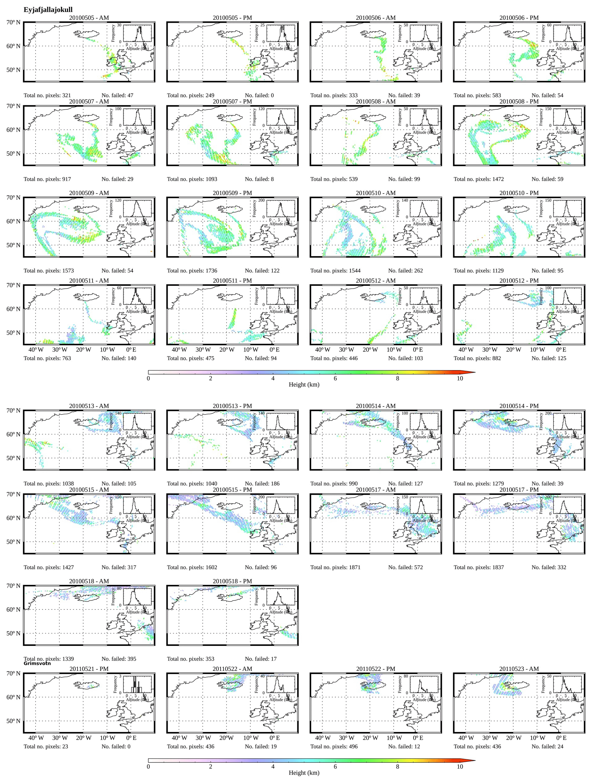
Figure 7 Maps of the CO₂ slicing output (with quality control applied) for the Eyjafjallajökull and Grímsvötn eruptions. Each plot consists of multiple orbits, divided into morning and afternoon. On each plot is a histogram showing the distribution of heights for each scene. Beneath each plot are numbers showing the total number of pixels in each image and the number of pixels for which the CO₂ slicing method was unable to return a value.

5.2 Comparison of results

The CO₂ slicing technique was applied to IASI ash flagged pixels from 13 and 3 d from the Eyjafjallajökull and Grímsvötn eruptions respectively. Maps of these results, with the orbits divided into morning and afternoon, are shown in Fig. 7. For each map there is a histogram showing the distribution of the retrieved heights. Encouragingly, initial examination of the maps shows that the retrieved values are spatially consistent with only a few outliers. These outliers are usually individual pixels whose altitudes are higher than those surrounding them. Below each map are numbers indicating the total number of pixels in each plot and the number of pixels for which the CO₂ slicing technique was unable to obtain a height, either because there is no intersection between the two functions shown in Eqs. (1) and (2) or because of the failure of one or more of the quality control measures outlined in Sect. 4. Overall, the CO₂ slicing technique was able to obtain a height value for 88 % of pixels from the two eruptions.

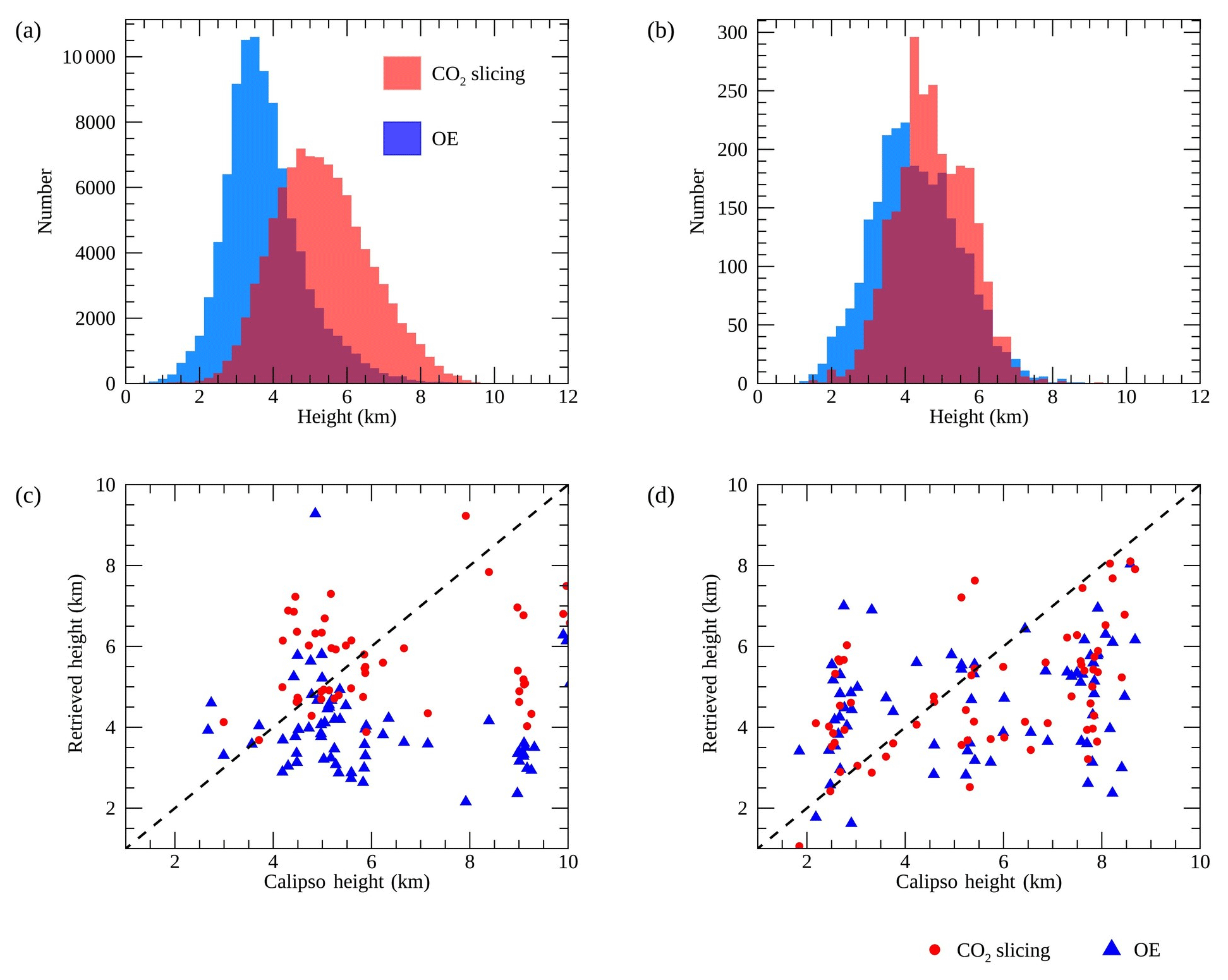
Figure 8 (a) Distribution of the CO₂ slicing and optimal estimation retrieved ash heights for all pixels from the Eyjafjallajökull eruption. (b) Same as (a) for the Grímsvötn eruption. (c) Comparison of the CALIOP heights with those obtained with the CO₂ slicing and optimal estimation techniques for a subset of pixels (where measurements fell within 50 km and 2 h of each other) from the Eyjafjallajökull eruption. (d) Same as (c) for the Grímsvötn eruption. Related statistics can be seen in Table 5.

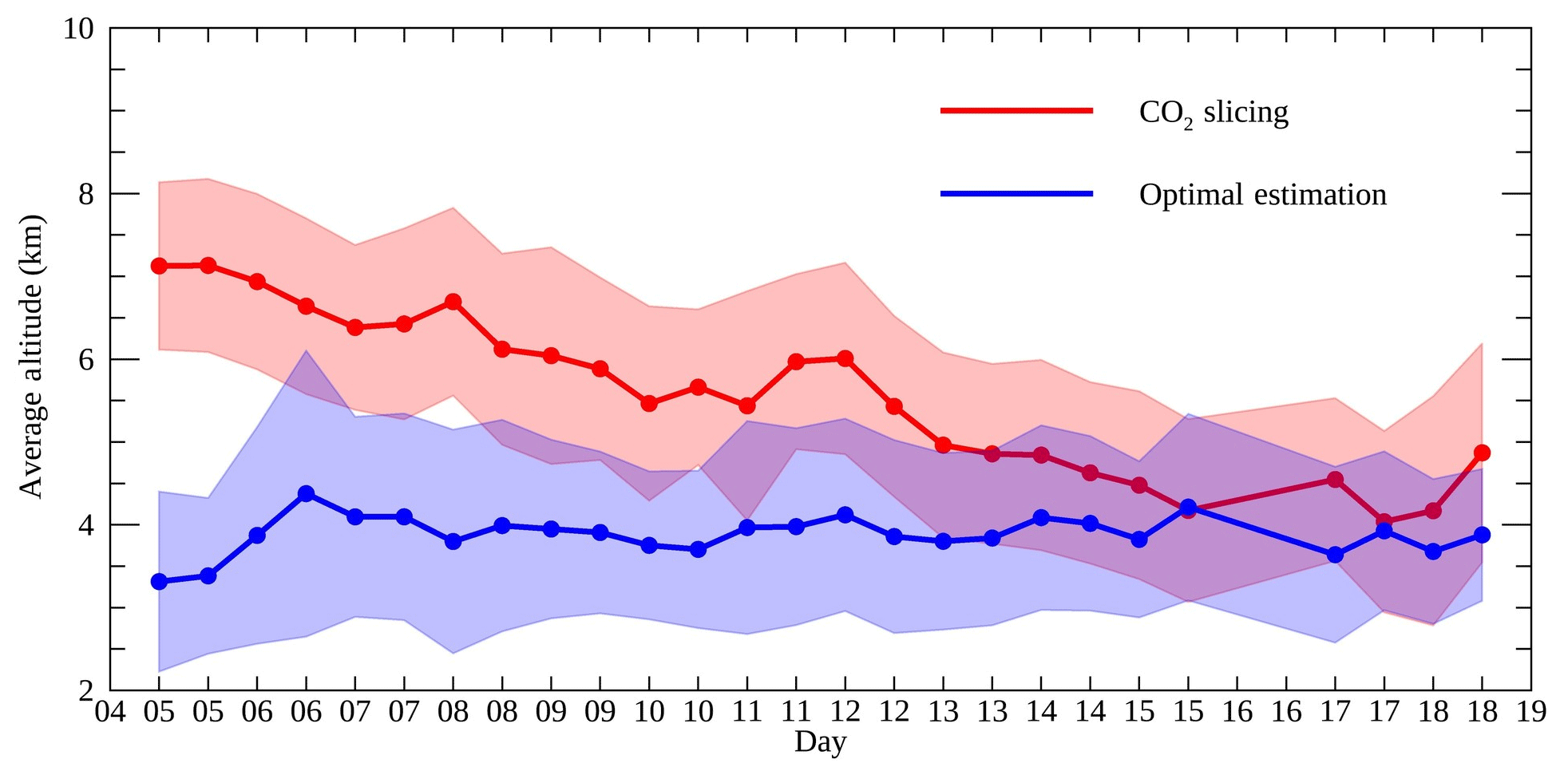
Figure 9 Time series showing how the average retrieved height for the CO₂ slicing and optimal estimation techniques varies during the Eyjafjallajökull eruption. The shaded polygon represents 1 standard deviation from the mean.

The CO₂ slicing results have been compared against those obtained with an optimal estimation (OE) scheme. Distributions of the heights obtained for all pixels from the two eruptions are shown in Fig. 8a and b. In both cases, the peak of the distribution for the CO₂ slicing heights is higher than for the OE scheme. Figure 9 shows how the average height obtained with the two retrievals has changed over the 13 d studied from the Eyjafjallajökull eruption. This plot shows that on 5 May the CO₂ slicing method retrieved an average altitude of roughly 7 km and that this then fell throughout the remainder of the study period. This corresponds to observations made about the volcano's activity. Activity at the volcano became more explosive on 5 May 2010 with increased emission of ash and SO₂, with plumes rising to greater than 8 km. This was followed by a fall in the plume height to 6–7 km, interspersed with higher plumes during more explosive activity (Petersen, 2010). The average CO₂ slicing heights shown in Fig. 9 are probably lower because these are values for the entire plumes including further away from the source. However, it does capture the changing elevation of the plume throughout the eruption. By contrast, the OE average heights are less variable: between 3 and 4.25 km throughout the period studied. Some example maps of the OE heights are shown in Figs. 10 to 13b, alongside the ash mass (panel c) calculated from the OE retrievals of AOD and effective radius, assuming an ash density. The maps of ash mass show that in general the ash mass falls with transportation away from the vent: the plumes become more disperse. The different design, assumptions and limitations of the two techniques mean that it is not expected that the two retrievals will return the same or even similar values. The optimal estimation scheme uses only 105 channels between 680.75 and 1204.5 cm⁻¹ (∼8.3–14.6 µm) to improve computational efficiency. This includes 14 channels within the CO₂ absorption band, only one of which is in common with the CO₂ slicing. However, unlike the CO₂ slicing method presented here, the channels used by the optimal estimation scheme have not been optimised for retrieving the height of the ash layer. Ventress et al. (2016) noted that the optimal estimation retrieval could be further refined by altering the channels used. For example, channels with more height information could be selected. Similarly, Ventress et al. (2016) suggested that channels could be selected to minimise the effect of the underlying cloud layers following observations that the OE method can underestimate the cloud top height in cases of multiple cloud layers (Ventress et al., 2016). In the current application of the optimal estimation scheme, where there is not sufficient information about the height of the ash layer within the channels used, the retrieval height output will tend to the a priori height which in this case is around 3.5 km. This is potentially the reason for the persistently lower average height shown in Fig. 9 which suggests a strong dependence on the a priori height. In future applications of the OE scheme, the CO₂ slicing results could be used as the a priori height if the one CO₂ channel that the two retrievals have in common was removed from the optimal estimation scheme. Other differences in the results may arise from the nature of the two techniques. The OE scheme returns values for the ash optical depth, effective radius and height by fitting simulated spectra to those obtained with IASI. Ventress et al. (2016) identified that in some cases the retrieval underestimated the altitude of the plume and obtained a high ash optical depth in order to fit the measured spectra when in reality the ash layer might have a lower optical depth and higher altitude.

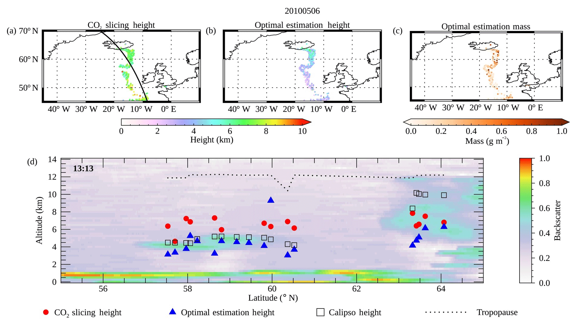
Figure 10 (a) CO₂ slicing results for 6 May 2010. Overplotted on this is the CALIPSO track. (b) The optimal estimation scheme heights. (c) The ash mass obtained with the optimal estimation scheme. (d) The CALIOP backscatter plot, with the CO₂ slicing results and the optimal estimation scheme heights plotted on top. Indicated on the top left-hand side of the plot is the time of the CALIOP overpass. The dashed line indicates the height of the tropopause.

Figure 11 Same as Fig. 10 for 9 May 2010.

Figure 12 Same as Fig. 10 for 22 May 2011.

Figure 13 Same as Fig. 10 for 23 May 2011.

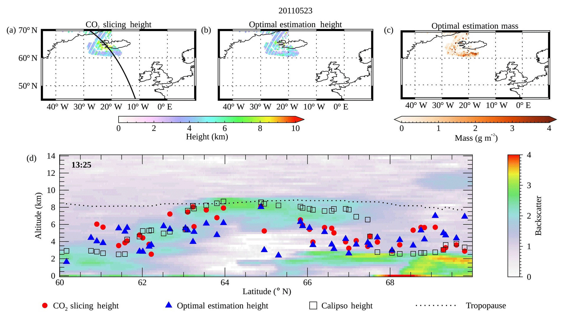
A comparison has been made against backscatter profiles and cloud altitudes obtained with CALIOP to assess how successfully the two retrievals perform. These backscatter profiles are shown in Figs. 10–13d. The heights obtained from the OE and CO₂ slicing methods for pixels which fall within 2 h and 50 km are overplotted, along with the heights obtained with CALIOP and the tropopause height. In these plots it is possible to observe that both methods are capable of capturing the height of the ash layer, but there are clear cases where one technique outperforms the other. In Fig. 10 which shows the backscatter plot for 6 May 2010, the CO₂ slicing method places the ash cloud between 5 and 7 km between 57.5 and 60.5^∘ N. This is shown to be higher than the CALIOP heights (4–5 km) to which the OE results are a closer match. In the same image, between 63 and 64^∘ N the CO₂ slicing results are again higher than the OE results but this time are closer to, but lower than, the heights obtained from CALIOP. The lower heights of both the CO₂ slicing and OE scheme relative to CALIOP might be related to the thick underlying cloud layer. Figure 11d shows another example from 9 May 2010. Here between 51 and 53^∘ N the heights obtained with both methods match those obtained with CALIOP. However, further north, between 56 and 60^∘ N, the CO₂ slicing results agree more closely compared to those from the OE scheme. At 66^∘ N, the CO₂ technique obtains a value close to the cloud top height, whereas the OE scheme obtains a value which is more representative of a lower layer of cloud. Figures 12 and 13 show examples from the Grímsvötn eruption and in both cases both height retrievals are shown to resemble the shape of the ash cloud layer shown by CALIOP. There are cases where both retrievals underestimate the cloud top height, which may be due to multiple layers of cloud.

Table 5 Statistics describing the comparison of the CO₂ slicing and optimal estimation scheme against the heights obtained with CALIOP.

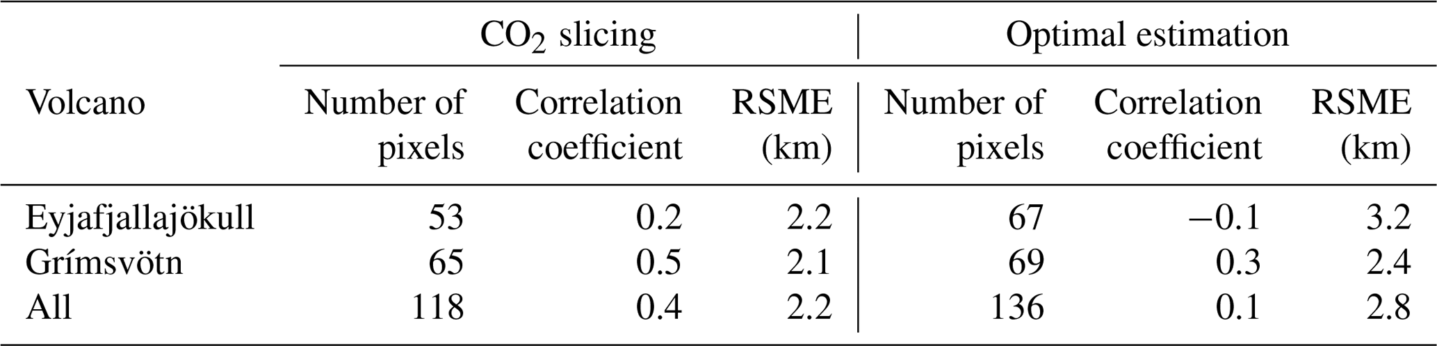
Pearson's correlation values and the RMSE were computed to compare the two retrieval methods against the heights obtained with CALIOP. These are shown in Table 5 and scatter plots comparing the retrieved values are shown in Fig. 8c and d. The Pearson correlation values are greater for the CO₂ slicing than for the OE scheme, while the RMSE values are lower: 2.2 and 2.1 km for the Eyjafjallajökull and Grímsvötn eruptions respectively for the CO₂ slicing technique, compared to 3.2 and 2.4 km obtained for the OE method. This implies an improved height retrieval from the CO₂ slicing method.

Although comparisons against lidar backscatter profiles are a common way of validating retrievals of ash and aqueous cloud height, these comparisons can be limited. CALIOP and IASI measure different things. The first measures backscattering while the latter measures thermal emission. Measurements are made with significantly different spatial resolutions (335 m compared to 12 km for CALIOP and IASI respectively) and in different locations (a maximum difference of 50 km). Clouds can also vary significantly in very short spaces of time. Although only pixels with a difference of 2 h have been considered in this comparison, this is still sufficient time for changes in the cloud's position both vertically and horizontally. These may account for some of the differences seen between the CALIOP profiles and the results obtained with the CO₂ slicing and the OE scheme. The cloud heights obtained from the CALIOP profile are not always a perfect representation of the cloud top height, which may also contribute to the differences observed. Although these limitations exist, comparisons against lidar instruments are still one of the best methods for validating cloud heights and in this case demonstrate that the CO₂ slicing technique has potential as a tool for obtaining the cloud top height of volcanic ash.

6 Conclusions

The CO₂ slicing technique is an established method, used for decades, for retrieving the cloud top height of aqueous cloud. Although it has previously been acknowledged that it can be applied to volcanic ash, it is not commonly used for this purpose, and it has only been applied to MODIS. In this study, the technique was adapted for IASI using simulated ash data to select the most appropriate channels and then demonstrate the technique's capability. When applied to the simulated data, the technique was shown to perform well in five out of six atmospheres. However, an increased failure rate was seen above and close to the tropopause and close to the surface. This was also true of ash with lower optical depths and effective radius. Similar observations have been made by previous CO₂ slicing studies. In this application three quality control criteria have been applied, which successfully remove the majority of cases where there are large differences between the true and retrieved pressures. When applied to ash scenes from the Eyjafjallajökull and Grímsvötn eruptions, the CO₂ slicing results compared well against the CALIOP backscatter profiles. It was also demonstrated that the CO₂ slicing method obtained heights which more closely matched CALIOP than the optimal estimation scheme used for comparison.

This is the first application of the CO₂ slicing technique to obtain the height of volcanic ash from IASI spectra, and the results are very encouraging. One advantage of this algorithm is that it can be run fairly quickly and so it could be applied to get a first approximation of the height, which could then be used to help assist hazard mitigation. It can also then be used as an input parameter into models of ash cloud propagation or as an a priori height in other retrieval schemes. There is also potential for the further development of this technique in the future. Previous applications to cloud have created synthetic channels (multiple channels averaged together) which could be used to further improve the algorithm and its sensitivity to lower-level clouds (Someya et al., 2016). It would also be possible to explore other options for selecting channels or obtaining the final cloud height. The channel selection in this study was based on simulated data in six different atmospheres; another avenue to explore would be the selection of atmospheric specific channel pairs. Further work would also help appreciate the strengths and limitations of this technique and therefore where its use is most appropriate.

Appendix A

Some additional figures are included within this Appendix. Figures A1 to A6 show the maximum difference between the true (simulated) and retrieved pressures for the six investigated atmospheres for all the channel combinations between 660 and 800 cm⁻¹. The plots are divided into the different pressure levels. The figure also includes the percentage of successful retrievals (where there is an intersections between the two functions shown in Eqs. 1 and 2 and all quality control conditions are met). This is out of a total of eight simulations (for each pressure level) with ash optical depths ranging between 5 and 15 and effective particle radius ranging between 5 and 10 µm. These could be used to select channels which are appropriate for specific climatologies. Figure A7 shows the final simulation result for each atmosphere without the quality control applied.

Figure A1 Simulation results for an RTTOV default atmosphere. The top two rows shows the maximum difference between the true (simulated) and retrieved pressures grouped into the different pressure levels. Each level consists of ash optical depths ranging between 5 and 15 and effective radius between 5 and 10 µm. The bottom two rows show the percentage of accepted retrievals (i.e. the percentage of cases where there is an intersection between Eqs. 1 and 2 and where all quality control criteria are met).

Figure A2 Same as Fig. A1 for a mid-latitude day atmosphere.

Figure A3 Same as Fig. A1 for a mid-latitude night atmosphere.

Figure A4 Same as Fig. A1 for a tropical atmosphere.

Figure A5 Same as Fig. A1 for a polar summer atmosphere.

Figure A6 Same as Fig. A1 for a polar winter atmosphere.

Figure A7 Same as Fig. 6 without a quality control applied.