the Creative Commons Attribution 4.0 License.
the Creative Commons Attribution 4.0 License.
 | 17 Jul 2019
Inversion of multiangular polarimetric measurements over open and coastal ocean waters: a joint retrieval algorithm for aerosol and water-leaving radiance properties
Peng-Wang Zhai
Bryan A. Franz
Yongxiang Hu
Kirk Knobelspiesse
P. Jeremy Werdell
Amir Ibrahim
Brian Cairns
Alison Chase
Ocean color remote sensing is a challenging task over coastal waters due to the complex optical properties of aerosols and hydrosols. In order to conduct accurate atmospheric correction, we previously implemented a joint retrieval algorithm, hereafter referred to as the Multi-Angular Polarimetric Ocean coLor (MAPOL) algorithm, to obtain the aerosol and water-leaving signal simultaneously. The MAPOL algorithm has been validated with synthetic data generated by a vector radiative transfer model, and good retrieval performance has been demonstrated in terms of both aerosol and ocean water optical properties (Gao et al., 2018). In this work we applied the algorithm to airborne polarimetric measurements from the Research Scanning Polarimeter (RSP) over both open and coastal ocean waters acquired in two field campaigns: the Ship-Aircraft Bio-Optical Research (SABOR) in 2014 and the North Atlantic Aerosols and Marine Ecosystems Study (NAAMES) in 2015 and 2016. Two different yet related bio-optical models are designed for ocean water properties. One model aligns with traditional open ocean water bio-optical models that parameterize the ocean optical properties in terms of the concentration of chlorophyll a. The other is a generalized bio-optical model for coastal waters that includes seven free parameters to describe the absorption and scattering by phytoplankton, colored dissolved organic matter, and nonalgal particles. The retrieval errors of both aerosol optical depth and the water-leaving radiance are evaluated. Through the comparisons with ocean color data products from both in situ measurements and the Moderate Resolution Imaging Spectroradiometer (MODIS), and the aerosol product from both the High Spectral Resolution Lidar (HSRL) and the Aerosol Robotic Network (AERONET), the MAPOL algorithm demonstrates both flexibility and accuracy in retrieving aerosol and water-leaving radiance properties under various aerosol and ocean water conditions.
- Article
(7210 KB) - Full-text XML
- Companion paper
- BibTeX
- EndNote


The ocean is of immense importance for Earth's climate and ecosystems, and its conditions have great economic and social impacts (Costanza, 1999). It is critical to monitor and evaluate oceanic biogeochemical properties on the global scales using approaches such as ocean color remote sensing (Chapman, 1996). For both spaceborne and airborne remote sensing of ocean color, atmospheric correction is an important procedure to extract the water-leaving optical signal from the total measurement of the coupled atmosphere and ocean system. Atmospheric correction algorithms in part estimate the aerosol path radiance and the ocean surface reflectance and remove them from the total signal. The remaining water-leaving signal is due to absorption and scattering inside the water body, which can be used to retrieve the optical properties of seawater constituents and infer their associated biogeochemical conditions (Mobley et al., 2016). Due to the small percentage of the water-leaving signals in the total measurement (Zhai et al., 2017), atmospheric correction requires precise evaluation of the aerosol and ocean surface contributions, which is very challenging when absorbing aerosols are present and when water-leaving signals in the near-infrared spectral region are non-negligible, both of which are often the case for coastal waters (Sathyendranath, 2000; Wang, 2010).
Multiangle, multispectral polarimeters (hereafter simply referred to as polarimeters) measure signals that contain rich information on aerosols and hydrosols (Chowdhary et al., 2005, 2012; Hasekamp et al., 2011; Knobelspiesse et al., 2012; Xu et al., 2016; Stamnes et al., 2018; Dubovik et al., 2019). The aerosol properties obtained from polarimeter data can be explored to improve the atmospheric correction for complex atmosphere and ocean systems (Jamet et al., 2019). In the Decadal Survey for Earth Science and Applications from Space proposed by the National Academy of Sciences for the years 2017–2027, a polarimetric imager is one of the top priority systems for aerosol observations (National Academies of Sciences, Engineering, and Medicine, 2018). Meanwhile, the National Aeronautics and Space Administration (NASA) plans to launch the Plankton, Aerosol, Cloud, ocean Ecosystem (PACE) mission in the 2022–early 2023 time frame (Werdell et al., 2019), which will carry the Ocean Color Instrument (OCI), a hyperspectral radiometer with continuous spectral coverage from the ultraviolet (350 nm) to near infrared (890 nm), plus a set of discrete shortwave infrared bands (940, 1038, 1250, 1378, 1615, 2130, and 2260 nm). In addition, PACE will carry two polarimeters: the Hyper-Angular Rainbow Polarimeter (HARP2) (Martins et al., 2014) and the Spectropolarimeter for Planetary EXploration (SPEXone) (Hasekamp et al., 2019). With this three-instrument payload, PACE will provide new opportunities to perform better atmospheric correction to the OCI imagery with the aerosol information retrieved by the colocated polarimeter measurements.
To extract the rich information contained in polarimeter measurements, several joint retrieval algorithms have been developed to determine aerosol and water optical properties simultaneously. Oceanic optical properties are usually solely parameterized by the concentration of the photosynthetic pigment chlorophyll a ([Chl a]) (Chowdhary et al., 2005; Hasekamp et al., 2011; Xu et al., 2016; Stamnes et al., 2018). Gao et al. (2018) proposed a joint retrieval approach, so called the Multi-Angular Polarimetric Ocean coLor (MAPOL) retrieval algorithm, for a coupled atmosphere and ocean system that employs a generalized bio-optical model for coastal waters. There are seven free parameters in this bio-optical model that describe the absorption and scattering characteristics of different components such as water, phytoplankton, colored dissolved organic matter (CDOM) and nonalgal particles (NAPs). The MAPOL retrieval algorithm was validated with synthetic data generated by a radiative transfer model (Zhai et al., 2009, 2010, 2015, 2017, 2018), which demonstrated high accuracy in the retrieval of water-leaving signals and aerosol microphysical properties for a large variety of atmospheric and ocean conditions. The purpose of this paper is to further validate the algorithm by applying it to airborne observations. Specifically, the retrieval algorithm processes the polarimeter measurements over both open and coastal waters and generates water-leaving signals as well as aerosol properties, which are then compared with in situ measurements to evaluate the accuracy and uncertainties.
In order to accurately fit the field measurements, the original MAPOL algorithm in Gao et al. (2018) has been further upgraded to include trace gas absorption and an updated instrument noise model. A [Chl a]-based bio-optical model has also been added to constrain the water-leaving radiance for open waters. Both the [Chl a]-based model and the general seven-parameter bio-optical model are applied over coastal waters in order to evaluate their impacts on the water-leaving signal retrieval. This work builds upon the polarimetric retrieval studies (Chowdhary et al., 2005, 2012; Dubovik et al., 2011; Hasekamp et al., 2011; Knobelspiesse et al., 2012; Xu et al., 2016; Stamnes et al., 2018) and extends the retrieval of ocean optical properties to coastal regions.
The paper is organized into six sections: Sect. 2 will introduce the data from field measurements used in the retrieval study, Sect. 3 will review the MAPOL retrieval algorithm, Sect. 4 presents the retrieval results, Sect. 5 discusses the results, and Sect. 6 summarizes the conclusions.
In this work, we have applied the MAPOL retrieval algorithm to the measurements acquired by the airborne Research Scanning Polarimeter (RSP) (Cairns et al., 1999; Knobelspiesse et al., 2019). RSP includes six boresighted refractive telescopes that formed three pairs, with each pair measuring three spectral bands (Cairns et al., 1999). Nine wavelengths are measured with the central wavelengths and band width at visible (VIS) bands: 410 (30), 470 (20), 550 (20), and 670 (20) nm; near-infrared (NIR) bands: 865 (20), and 960 (20) nm; and shortwave infrared (SWIR) bands: 1590 (60), 1880 (90), and 2250 (120) nm. The scanning direction relative to the instrument baseplate is within ±60∘ with 152 angles and an instantaneous field of view (IFOV) of 14 mrad (0.8∘), which can be geolocated to provide hyperangular measurements of the same target. For the measurements in our following discussion as summarized in Table 1, the spatial resolution is about 100 m which can be estimated from the product of the IFOV and aircraft altitude.
Within each pair of the telescopes, one makes measurements of the polarization components at the orthogonal plane of 0 and 90∘ denoted as and , and the other telescope simultaneously measures the polarization components at 45 and −45∘ denoted as and . The polarized measurement is denoted using a Stokes vector , where , , and Vt is usually negligible for the atmospheric studies. The total radiance used in this study is an average of the radiance remeasured by the two telescopes and is defined as . The corresponding instrument noise model is provided in Knobelspiesse et al. (2019) and summarized in Appendix B.
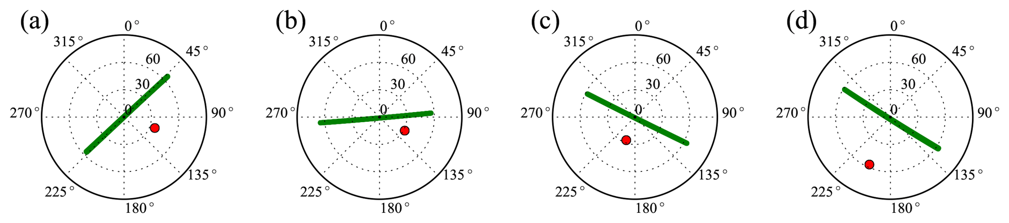
The measurements from two field campaigns are chosen for this study, namely the Ship-Aircraft Bio-Optical Research (SABOR) experiment and the North Atlantic Aerosols and Marine Ecosystems Study (NAAMES). The SABOR experiment was conducted from 17 July to 7 August 2014 (NASA SABOR webpage, 2019), and the NAAMES campaign is a multiyear study where four month-long expeditions took place between 2015 and 2018 (NASA NAAMES webpage, 2019). During both campaigns the airborne measurements from RSP and in situ measurements from the ocean vessels were acquired. Due to the difficulty of finding polarimeter observations in cloud-free conditions over the ocean with coordinated in situ water-leaving signal measurement, only four cases from SABOR and NAAMES are investigated in this study. Each case is given a name for our discussion by combining its campaign name and the water types: SABOR-Open, SABOR-Coastal, NAAMES-Open, and NAAMES-Coastal. The basic information for the measurements including the time, location, and instrument geometries is summarized in Table 1. The aerosol optical depth (AOD) from these cases ranges from 0.05 to 0.35. The corresponding RSP files are listed in Appendix . The locations and polar graphs of the solar direction and the RSP scanning direction for each case are summarized in Figs. 1 and 2.
Table 1Summary of datasets from the SABOR and NAAMES field campaigns. The case name is given as a combination of the campaign name and water types. The time range is for the start and end time of the corresponding RSP scene. The retrieval time, latitude, longitude, solar, and scattering geometry are for the RSP measurements in the corresponding field campaign. The time for the in situ measurement is also given for comparison. All time is in UTC. The altitude is the height of the aircraft which carried RSP. The relative azimuth angle is the relative angle between the RSP scanning direction and the principal plane formed by the solar direction and the zenith direction.
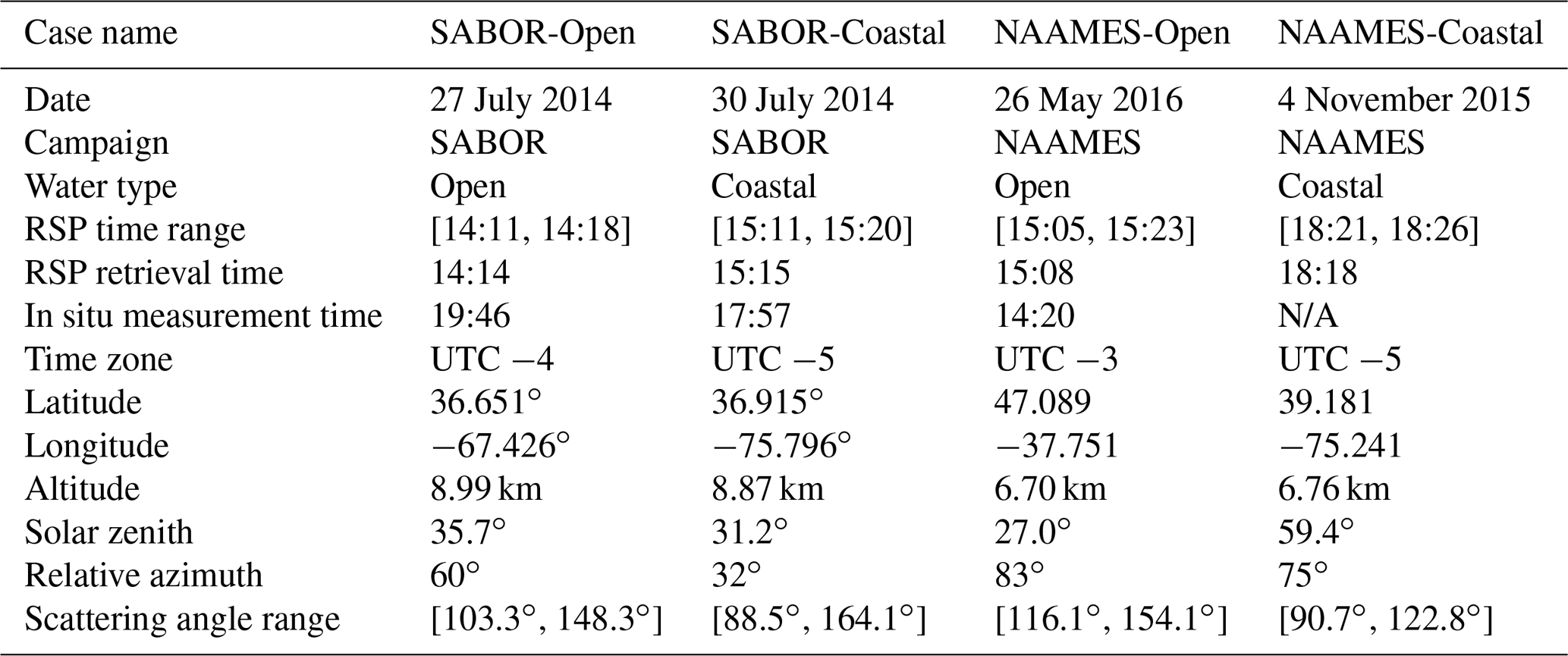
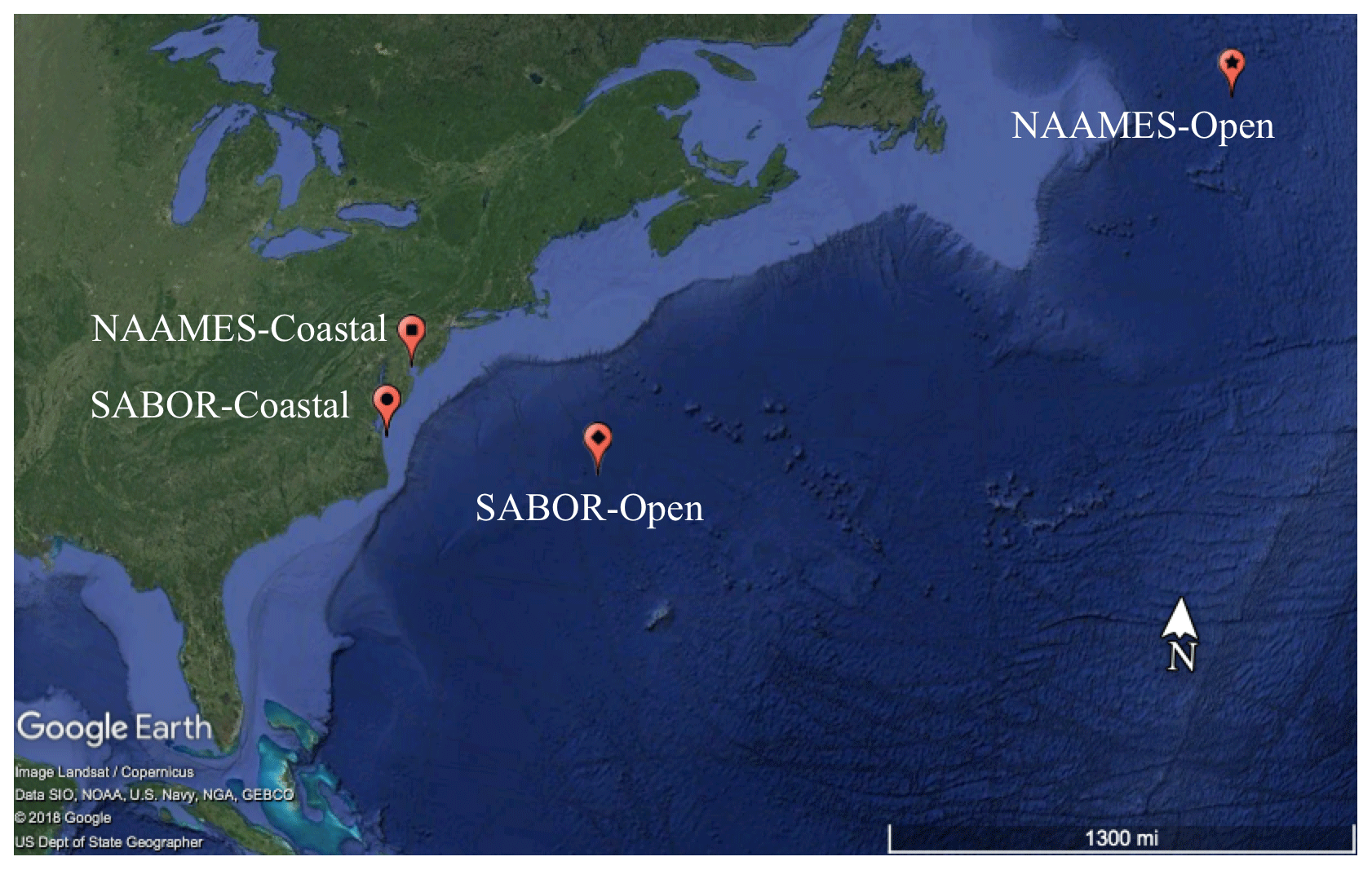
Figure 1The locations of the RSP measurements as listed in Table 1.
The MAPOL algorithm for simultaneous aerosol and water optical property retrieval is based on the multiangle, multiwavelength, and polarization measurements. In the following, we will first introduce the definition of the measurement and retrieval quantities. The retrieval algorithm implements an optimization approach that minimizes the difference between the measurements and the forward model simulations, formally defined as the cost function in Eq. (3) below. The forward model is the radiative transfer model that computes the reflectance at sensor level using both aerosol and ocean bio-optical models as reviewed in the previous study (Gao et al., 2018; Zhai et al., 2010).
3.1 Reflectance and remote sensing reflectance
Using the measured Stokes vector components, the total reflectance ρt and polarized reflectance ρP at sensor level are defined as
where F0 is the extraterrestrial solar irradiance, μ0 is the cosine of solar zenith angle, and r is the solar distance in astronomical units. The total reflectance ρt includes contributions from the molecular (Rayleigh) scattering ρR, aerosol scattering ρa, the interaction term of Rayleigh and aerosol ρRa, surface reflectance such as sunglint ρg and whitecaps ρwc, and the water-leaving contributions ρw. In ocean optics literature, L is often used to denote radiance which is the same as I in a Stokes vector (Mobley, 1994). The objective of the atmospheric correction is to obtain ρw by removing all other contributions – this requires accurate modeling of the molecular and aerosol scattering and the surface reflectance.
Remote sensing reflectance, defined as , is commonly used to represent the water-leaving signal originating from scattering from the water body, where is the upwelling water-leaving radiance just above the water surface after the atmospheric correction and is the downwelling irradiance just above the water surface. The superscript is used to denote just above/below the ocean surface. The nadir direction is used to compute the remote sensing reflectance. The observed water-leaving reflectance at the airborne or spaceborne sensor is denoted as , which represents the water-leaving reflectance just above ocean surface transmitted to the sensor through a diffuse transmittance tu. can be obtained from the total reflectance measured at the sensor by removing the contribution from molecular and aerosol path radiance, ocean surface reflectance (e.g., sunglint, white caps), and their interaction terms (Gao et al., 2018). The remote sensing reflectance can be related to the water-leaving reflectance as
where td is the same as tu but represents the downward transmittance of the solar irradiance to the water surface (Gao et al., 2000). This definition is used in our study to conduct the atmospheric correction and calculate the remote sensing reflectance. A detailed mathematical treatment is in Appendix A.
3.2 Retrieval algorithm
In the MAPOL algorithm an optimization approach is used to retrieve the aerosol and ocean optical properties, where the measured reflectance is compared with the reflectance computed from a forward model using a set of parameters that specify the aerosol and ocean optical properties. If the agreement is within a predefined criterion, the optimization procedure finishes; otherwise, the retrieval parameters are updated and the whole process iterates until the convergence criterion is satisfied. The optimization algorithm used in the retrieval is the Levenberg–Marquardt method (Moré et al., 1980), where the Twomey–Tikhonov regularization is assumed implicitly (Moré, 1978; Rogers, 2000). A least squares cost function is defined to quantify the difference between the measurement and the simulation from a forward model as
where ρt and ρP are the measured reflectance defined in Eq. (1), and denote the reflection simulated from a forward model specified by a parameter vector x, i indicates the measurement at different angles and wavelengths, and N is the total number of the measurements used in the retrieval. The total uncertainties of the reflectance and the polarized reflectance are denoted as σt and σP (Knobelspiesse et al., 2019). The total uncertainty includes the instrument measurement uncertainties as discussed in Appendix B; the variance from averaging nearby RSP pixels (5 pixels are used in this study, which corresponds to a surface pixel size of approximately 500 m); and the modeling uncertainties with an estimated percentage error similar to the measurement uncertainty. More details of the MAPOL retrieval algorithm were discussed in Gao et al. (2018).
(Cox and Munk, 1954)Table 2The forward model for aerosol refractive index, volume distribution and ocean surface properties, and the parameters used for retrieval.
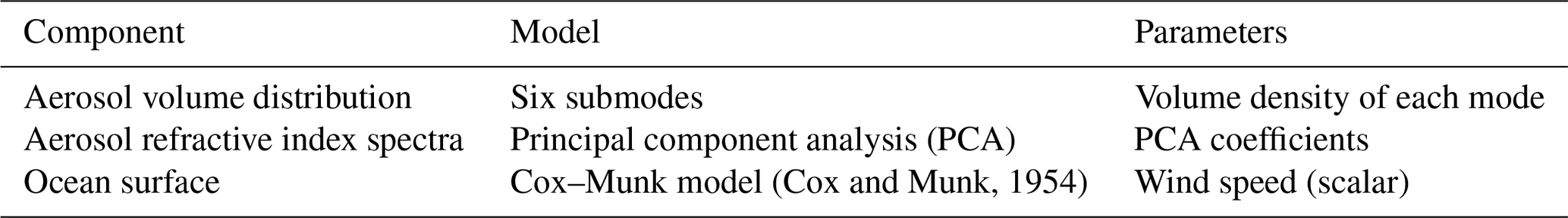
The forward model in the retrieval algorithm describes radiative transfer in the coupled atmosphere and ocean system. The atmosphere and ocean system are divided into three layers, with a top molecular layer, a middle layer filled by a mixture of molecules and aerosols, and then an ocean layer with a rough water interface. The aerosol top height is assumed to be 2 km in this work. The aerosol and ocean surface representations are summarized in Table 2, where the aerosol volume distribution is represented as the summation of six size modes with three submodes of fine-mode aerosols and another three submodes of coarse-mode aerosols (Gao et al., 2018). The complex aerosol refractive index spectra for fine and coarse mode are represented by the principal component analysis (PCA) of aerosol refractive index spectral measurements (Shettle and Fenn, 1979; d'Almeida et al., 1991; Wu et al., 2015). Only the major spectral variation represented by the first order of the principle components is considered (Gao et al., 2018). The PCA coefficients for both the real and imaginary refractive indices are retrieved from the algorithm. In the study of the SABOR-Coastal case, where the aerosol loading is relatively large, we also compare the results between the PCA representation and a more flexible representation of combining PCA with small adjustments in the refractive indices for the wavelengths of 410 and 470 nm in order to assess the possible cause of the bias at shorter wavelengths. Implementation details of the refractive index adjustment will be discussed with the SABOR-Coastal case. Moreover, in order to model the field measurement, the previous forward model (Gao et al., 2018) is further developed in this study by including the gas absorption due to ozone, oxygen, water vapor, nitrogen dioxide, methane, and carbon dioxide (Zhai et al., 2018). The aerosol scattering and absorption properties are then mixed with the gas absorption within the molecular and aerosol mixing layer.
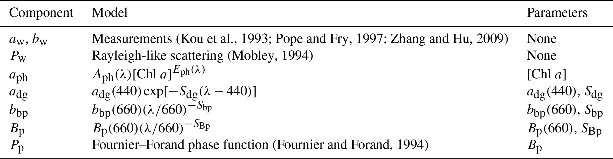
Bio-optical models can be used to describe the scattering and absorption of the key constituents in ocean waters including pure water, phytoplankton, CDOM, and NAP (Mobley, 1994). The pure seawater absorption and scattering coefficients (aw, bw) are obtained from measurements (Kou et al., 1993; Pope and Fry, 1997; Zhang and Hu, 2009), and the pure seawater phase function Pw is similar to Rayleigh scattering (Mobley, 1994). To model the coastal water optical properties, our bio-optical model considers seven parameters that explicitly define the scattering and absorption properties from phytoplankton, CDOM, and NAP (Gao et al., 2018). The key absorption and scattering properties are summarized in Table 3, which includes the absorption coefficients of phytoplankton (aph), the total absorption coefficient of CDOM and NAP (adg), the total particulate backscattering coefficient (bbp) for both phytoplankton and NAP, and the total particulate backscattering fraction defined as where bp is the particulate scattering coefficient. aph is a function of [Chl a] with coefficients Aph and Eph provided in Bricaud et al. (1998). The particulate phase function (Pp) is described by the Fournier–Forand phase function, which is an analytical function that can be determined by the backscattering fraction of Bp (Fournier and Forand, 1994). To obtain the total Mueller matrix of water, the particulate phase function is mixed with the water phase function and then multiplied by the normalized Mueller matrix derived from measurements (Voss and Fry, 1984; Kokhanovsky, 2003) where the polarization properties are assumed to be invariant.
(Kou et al., 1993; Pope and Fry, 1997; Zhang and Hu, 2009)(Mobley, 1994)(Fournier and Forand, 1994)Table 3The generalized ocean bio-optical model (Bio-2) for coastal waters.
When studying open waters, it is often assumed that [Chl a] can be used as a single parameter to describe the optical properties of all seawater constituents (Chowdhary et al., 2012; Xu et al., 2016). For open waters, we therefore constrain the parameters in the previously described bio-optical model using only [Chl a]. Specifically, the parameters describing adg(440), Sdg, bbp(660), Sbp, and Bp are respecified in terms of [Chl a] as shown in Appendix C. It is assumed that no contribution from NAP is significant in open ocean waters. In practice, we use the [Chl a]-based bio-optical model (Bio-1) in the open ocean to reduce uncertainties associated unnecessarily with multiple parameters, while we use the full seven-parameter bio-optical model (Bio-2) in coastal waters. We then evaluate the difference in using both the two bio-optical models for coastal water studies in order to understand the applicability of the different model parameterizations. We acknowledge that alternate parameterizations exist, but a detailed exploration of them exceeds the scope of this paper. Furthermore, if there is a priori knowledge of the parameters in the generalized bio-optical model, the number of retrieval parameters can be reduced by assuming prespecified values. For example, a similar bio-optical model for adg and bbp has been proposed in a spectral optimization approach (Kuchinke et al., 2009), where the spectral coefficients Sdg and Sbp are assumed to be known from existing studies. The reduced number of free parameters may help reduce uncertainties in the retrieved quantities.
The MAPOL retrieval algorithm discussed in the last section is applied to the RSP data acquired in the SABOR and NAAMES campaigns. Two locations are selected in each campaign: one for open ocean waters and the other for coastal ocean waters as summarized in Table 1. The [Chl a]-based bio-optical model (Bio-1) is applied to the open water cases, while both the [Chl a]-based bio-optical model (Bio-1) and the seven-parameter bio-optical model (Bio-2) are applied to the coastal water cases to explore the impact of model parameterization in the atmospheric correction.
For the SABOR measurements, we compared the retrieved aerosol optical depth with the aerosol product from the High Spectral Resolution Lidar (HSRL) (Hair et al., 2008) and the Aerosol Robotic Network (AERONET) (Holben et al., 1998). The collocated in situ measurements of the water-leaving signals are compared with the retrieval results from SABOR-Open, SABOR-Coastal, and NAAMES-Open. For NAAMES-Coastal, there are no in situ measurements available; instead we compared with the ocean color product derived from the Moderate Resolution Imaging Spectroradiometer (MODIS) on board Aqua.
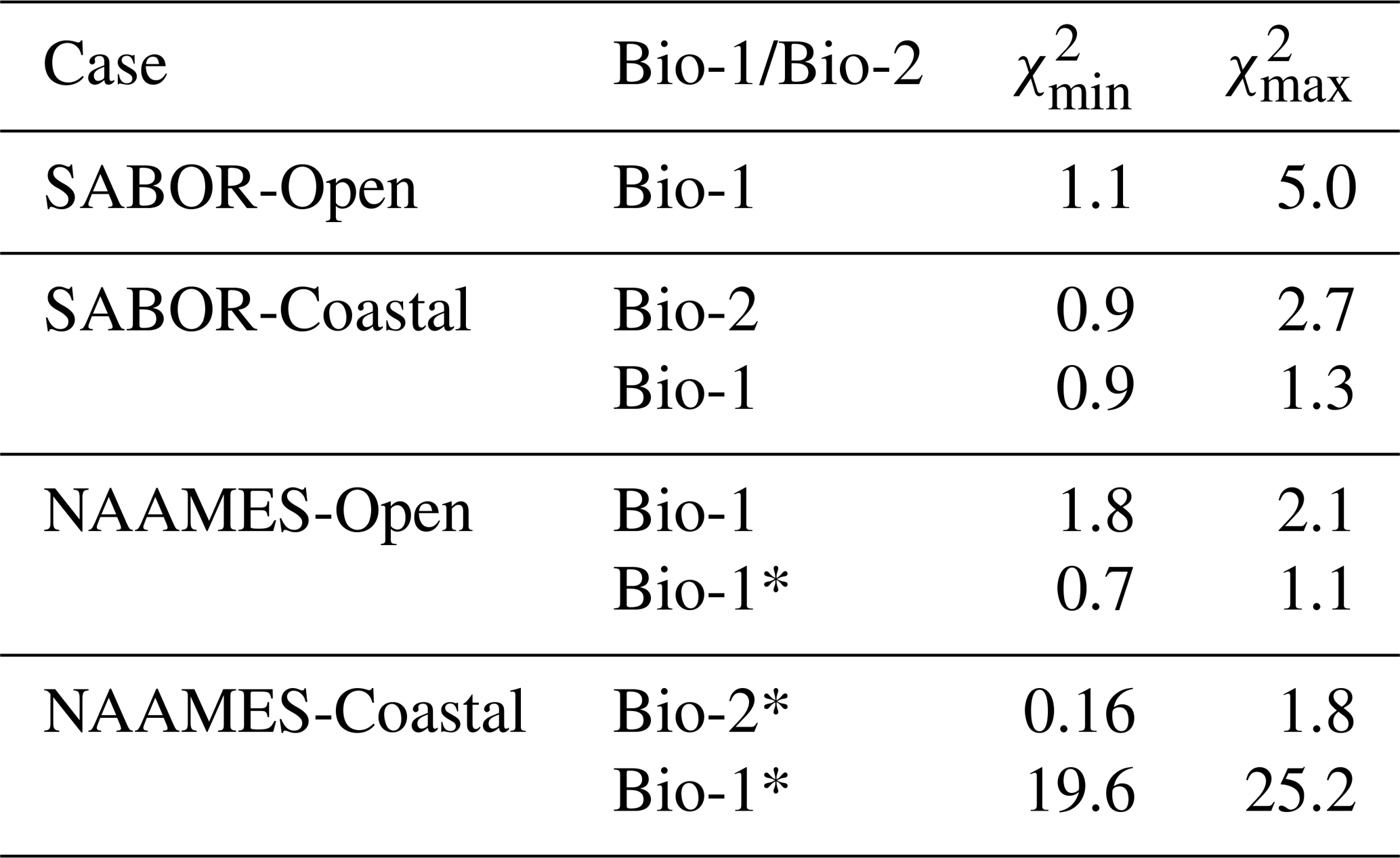
The χ2 value of a converged case indicates the retrieval quality. A χ2 close to 1 means that the average difference between the measurement and the simulation is comparable to the uncertainty model quantified by σt and σP (Rogers, 2000). If χ2 is much larger than 1, it may suggest underfitting, where the forward model does not sufficiently describe the measurements. For example, this could indicate that the measurements are influenced by clouds and should be carefully screened (Stap et al., 2015). In practice, since the retrievals cannot always reach the global minimum due to the local minima of the cost function, the converged χ2 value depends on the initial values of the retrieval parameters. In order to explore the corresponding retrieval uncertainties, we ran the retrieval algorithm 50 times for each case listed in Table 1. Each time the initial values of the retrieval parameters are different and randomly generated. The cumulative probability (CP) of all 50 converged χ2 values is evaluated. The 1σ uncertainties of the retrieval parameters can be determined by the range of variability of all retrievals with χ2 smaller than that of CP = 70 %. Within this CP, the minimum and maximum cost function values are denoted as and , corresponding to the best and worst fitted simulations, respectively. For the four cases in our study, the and are summarized in Table 4. The implications of χ2 values and retrieval uncertainties due to initial values will be discussed in detail for each case in the following sections.
Table 4The minimum and maximum values, and , for CP = 70 % with the two bio-optical models and the four cases listed in Table 1. Bio-1 is applied for open waters, while both Bio-2 and Bio-1 are applied for coastal waters. All cases use the seven RSP bands except for the ones indicated by an asterisk which did not use SWIR bands.
4.1 SABOR-Open waters (27 July 2014)
During the SABOR 2014 field campaign, RSP measurements were made from the NASA LaRC's King Air UC-12B aircraft at heights around 9 km over the Atlantic region across both open and coastal waters (Ottaviani et al., 2018). HSRL was also on board the aircraft, providing accurate aerosol optical depth information that is useful to validate the retrieved aerosol properties from our model. Coordinated in situ measurements from the R/V Endeavor provided water-leaving reflectance at various locations for both open and coastal waters. On 27 July 2014, the vessel for the SABOR-Open case was located near 700 km away from the coast as shown in Fig. 1. The in situ measurements of water-leaving signals were collected using a Satlantic HyperPro tethered in buoy mode (Chase et al., 2017). In this study we compared our retrieval results with these HyperPro measurements, all of which are available from NASA's SeaBASS (NASA SeaBASS webpage, 2019). The upwelling radiance Lu is measured at a depth of 0.2 m below ocean surface and then extrapolated to just below the ocean surface (). The upwelling radiance just above the water surface can be estimated as
where T is the transmittance from just below the water surface to just above the water surface with a value of 0.98 and the nw is the water refractive index with a value of 1.34. The remote sensing reflectance is then computed using for the comparison with the retrieval results.
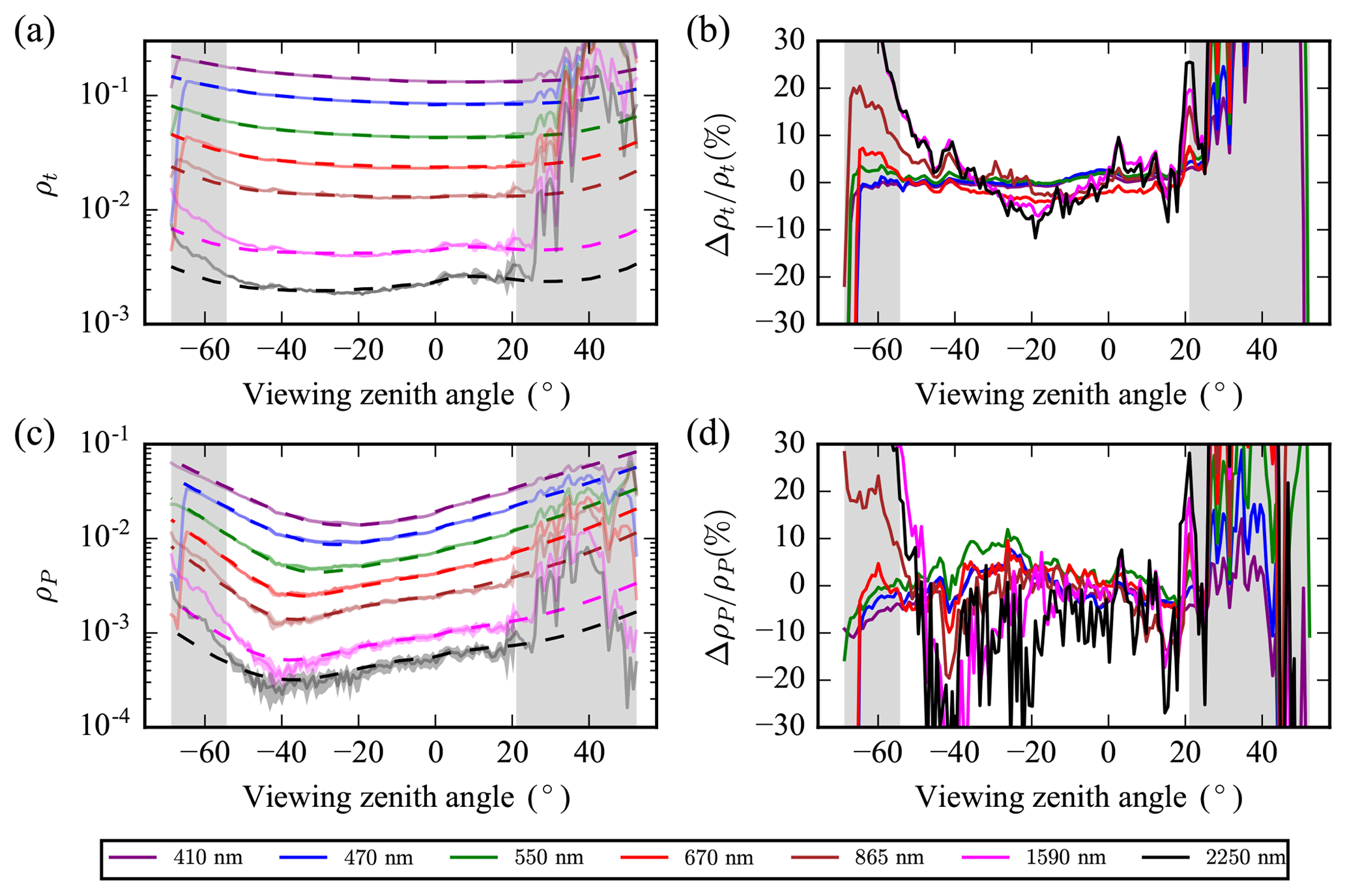
Figure 3(a) The comparison of the RSP measurement and simulation reflectance ρt for the SABOR-Open case at 14:14 UTC; (b) the relative differences; (c) and (d) are the same as for (a) and (b) but for polarized reflectance ρP. The solid line is the measurement data with vertical line width as measurement uncertainties. The dashed line is the simulation results from the retrieval. The gray-area-covered angles were not used in the retrieval. The minimum cost function value is , and the bio-optical model used in this retrieval is the Bio-1 model.
The solar and viewing geometry is summarized in Table 1 for the SABOR-Open case and is also shown in the polar plot of the geometry in Fig. 2 with a solar zenith angle of 35.7∘. The RSP viewing directions are away from the principal plane by a relative azimuth angle of 60∘ on average. As shown in Fig. 3, the measured reflectance does not contain a prominent sunglint reflection peak. The solid lines with a vertical spreading indicate the measurement with uncertainties. A portion of directions are influenced by clouds that are masked out in gray color in Fig. 3 and excluded from the retrieval.
The retrieval algorithm with Bio-1 is applied on the measurements as indicated by the solid line in Fig. 3a and c. The maximum cost function value is . The corresponding retrieval uncertainties for AOD and remote sensing reflectance are calculated as discussed previously. The best fitted simulation result is shown in Fig. 3a and c by the dashed line with . The percentage difference between the measurement mean value and the simulation results is shown for both reflectance and polarized reflectance (ρt and ρP) in Fig. 3b and d. Among most angles, the percentage difference for ρt is less than 5 %, but there are slightly larger percentage errors up to 10 % for SWIR bands at a few angles. For ρP, the overall percentage difference is less than 10 %, except for the SWIR bands where the largest percentage difference around −40∘ can go beyond 30 % due to the small polarized reflectance less than 10−3.
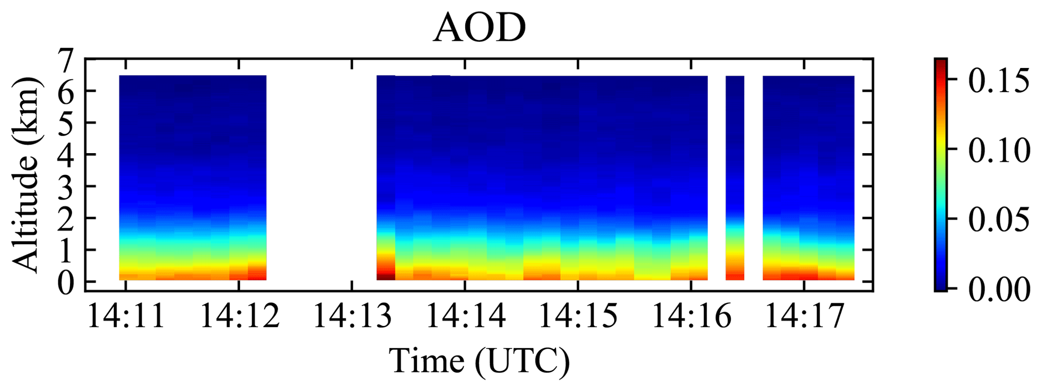
Figure 4The cumulative aerosol optical depth (AOD) at 532 nm from HSRL, which is the AOD of the layer from the aircraft to the altitude as indicated in the plot, for the open water case in 27 July 2014. The white stripes indicate no HSRL retrieval due the presence of cloud.
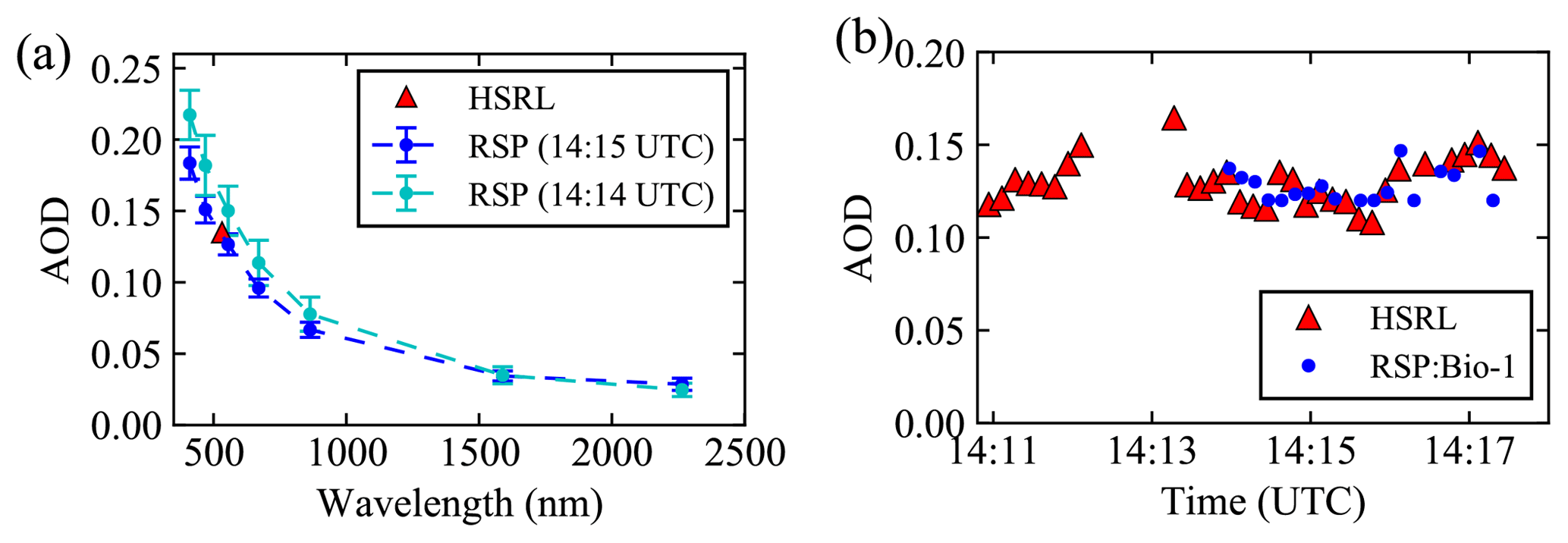
Figure 5(a) The retrieved aerosol optical depth (AOD) from RSP measurement at 14:14 UTC (SABOR-Open) and 14:15 UTC compared with a similar HSRL AOD at both times. The error bars indicate the retrieval uncertainties. The retrieval algorithm is based on the [Chl a]-based bio-optical model (Bio-1). (b) The comparison of the RSP-retrieved AOD at 550 nm with the HSRL AOD across the flight track.
HSRL provided complementary measurements of the aerosol optical depth, which can be used to validate our RSP retrievals. The vertical cumulative profile of HSRL AOD is shown in Fig. 4, where aerosols are mostly located with a vertical region within 1km from the surface. The retrieved aerosol optical depth spectrum from RSP is compared with HSRL optical depth in Fig. 5a. At 14:14 UTC, the averaged RSP AOD at 550 nm is 0.15, which is larger than the HSRL AOD value (0.135). The difference is smaller than the 1σ uncertainty of the RSP AOD retrieval, which is 0.017. HSRL observes a vertical profile of the aerosols as shown in Fig. 4, while RSP observes multiple viewing angles around ±60∘ relative to the instrument base plate. Near 14:13 UTC, a location 4.86 km away the SABOR-Open case, HSRL AOD is larger with a value of 0.164 as shown in Fig. 5b, which may contribute to the different RSP-observed AOD. Moreover, a nearby cloud may still influence the remaining angles of the RSP measurement through multiple scattering even after masking the obvious cloud-impacted region. To assess this hypothesis, we considered a location at 14:15 UTC, which is further away from the SABOR-Open case by 6.66 km. Here, the HSRL AOD is the same as the SABOR-Open case with a relatively clean and smooth variation in the nearby region as shown in Fig. 4. The retrieved aerosol optical depth at 550 nm has a better agreement with the HSRL AOD as shown in Fig. 5a, and the retrieval uncertainties reduce from 0.017 to 0.009.
Using the averaged retrieved aerosol properties at 14:15 UTC as the initial value, the retrieval algorithm is applied to the RSP measurement along the flight track. Figure 5b shows the comparison between the RSP and HSRL AOD, which demonstrates consistency. No RSP retrieval is shown around 14:12 to 14:13 UTC due to the large influence of cloud in the measurement.
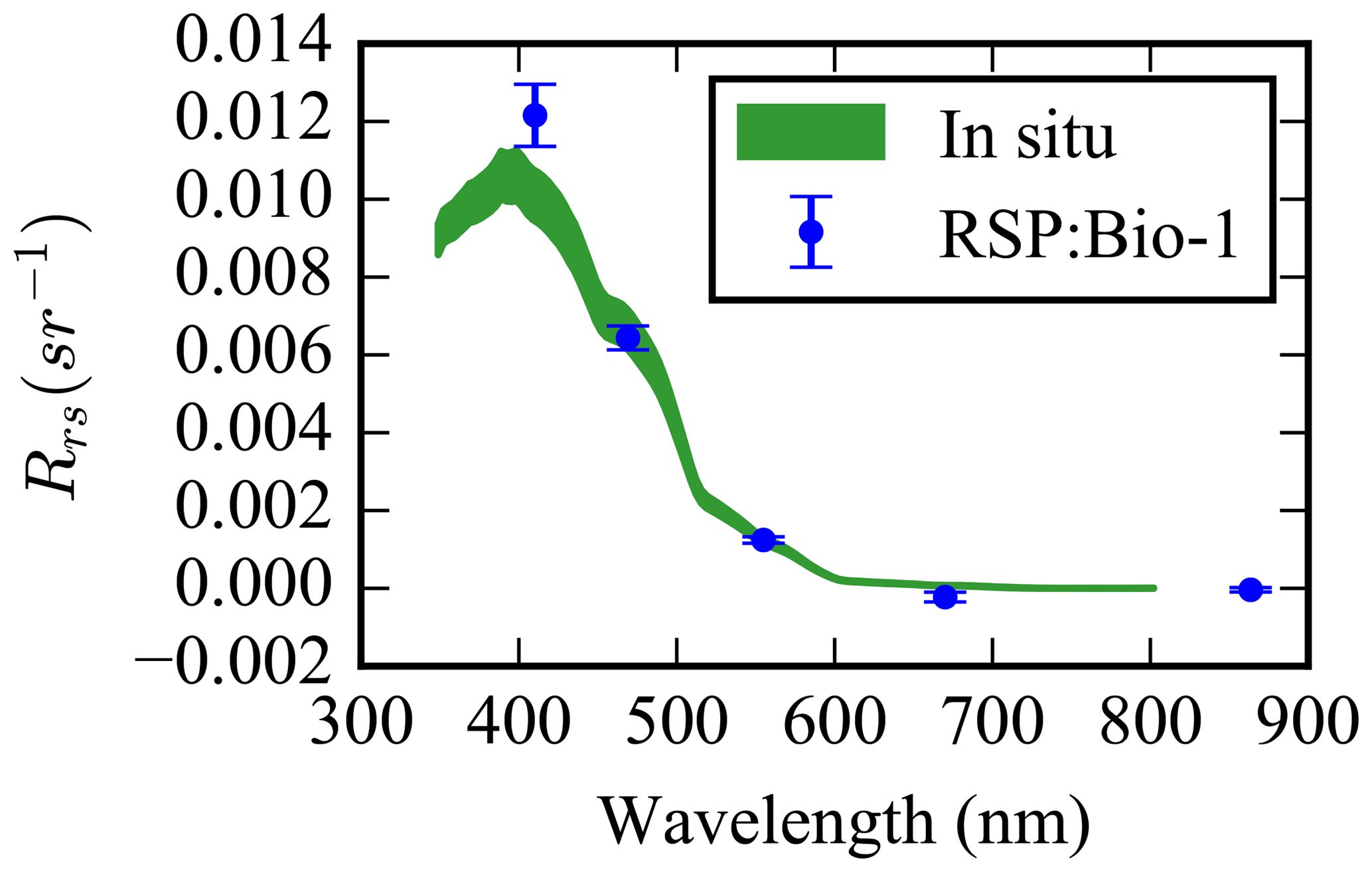
Figure 6The comparison of the RSP-retrieved remote sensing reflectance with the in situ measurements for SABOR-Open on 30 July 2014. The vertical line width indicates the uncertainties of the in situ measurements, while the error bars indicate the retrieval uncertainties.
The retrieved remote sensing reflectance is compared with the in situ measurement as shown in Fig. 6. The 1σ uncertainty of the in situ measurement is indicated by the vertical line width, which was calculated using the signal variability within the 5 min measurement duration. The RSP measurement was made at 14:14 UTC and the in situ measurement was made at 19:46 UTC as summarized in Table 1. The distance between these two locations is less than 0.1 km. The vertical bar indicates the RSP retrieval uncertainties. The maximum remote sensing reflectance obtained from the in situ measurement is 0.0106, while the Rrs from the RSP retrieval has a peak at 410 nm with a value of 0.0122. The retrieval uncertainty at 410 nm has a value of 0.00080, while the uncertainty for 470 nm is 0.00031, and for other bands it is less than 10−4. Figure 6 shows that our remote sensing reflectance agrees with the in situ measurements for all wavelength bands longer than 470 nm. At 410 nm, the difference is the largest, which is however acceptable due to inherent retrieval uncertainty associated with the large reflectance signal and the possible small-scale variability of ocean optical properties at deep blue wavelengths.
4.2 SABOR-Coastal waters (30 July 2014)
On 30 July 2014 during the SABOR campaign, R/V Endeavor was located 20 km away from the coast with in situ measurements available as shown by the SABOR-Coastal location in Fig. 1. We executed the joint retrieval of the aerosol properties and water-leaving reflectance using both the [Chl a]-based bio-optical model (Bio-1) and the seven-parameter bio-optical model (Bio-2). The retrieved properties are compared with the in situ measurement from HyperPro and the AOD product from HSRL and AERONET.
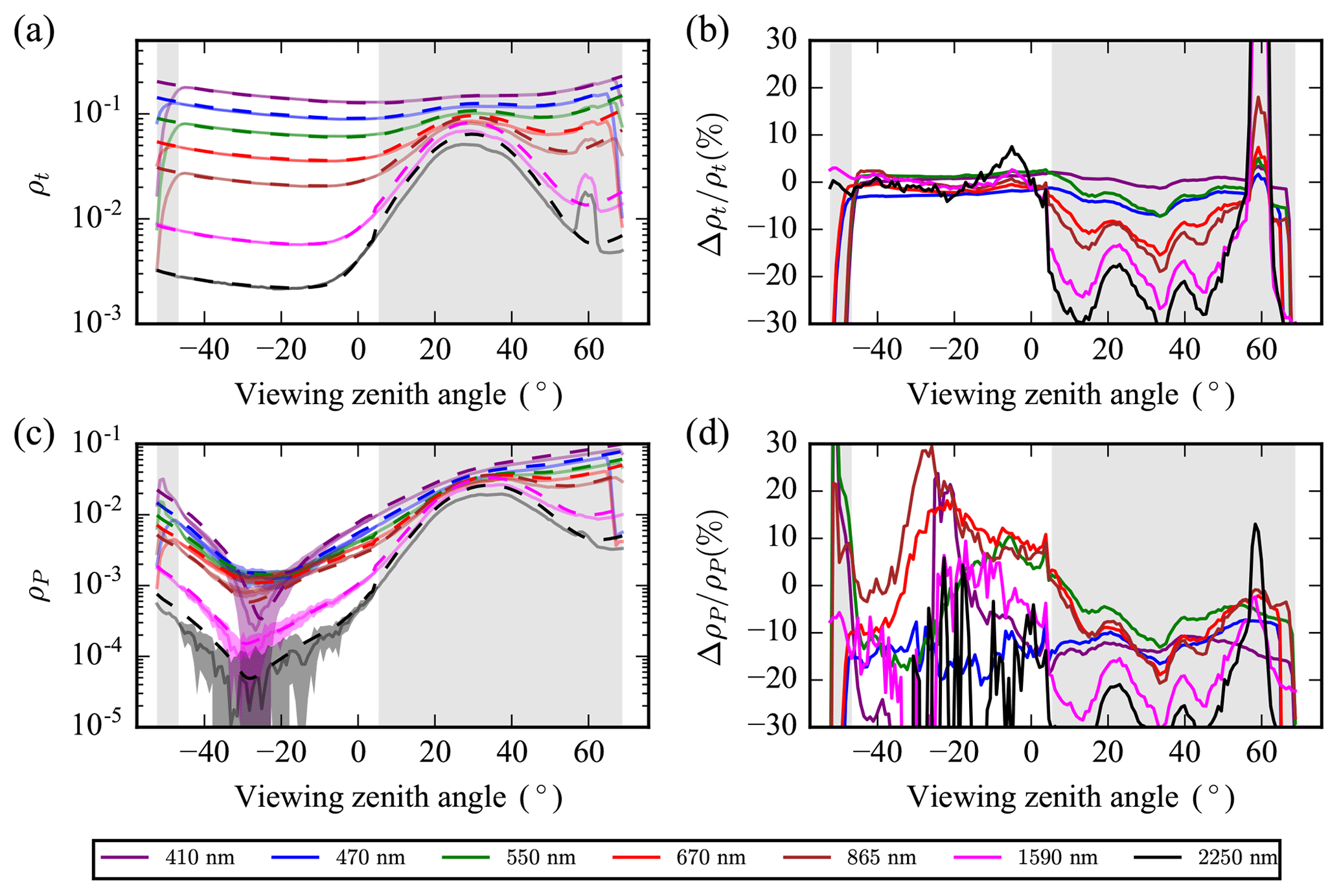
Figure 7Same as Fig. 3 but for SABOR-Coastal on 30 July 2014. The minimum cost function value is and the bio-optical model used here is Bio-2.
The solar zenith angle is 31.2∘ and the relative azimuth is 32∘ between the RSP scanning direction and principal plane for the SABOR-Coastal case, as shown in Fig. 2b and in Table 1. Figure 7 shows the comparison between the RSP-measured and model-fitted polarized reflectance field. As shown in Fig. 7a, the sunglint is prominent in the measurement data. A test retrieval with the sunglint considered produces a larger aerosol optical depth and larger aerosol absorption as compared with AERONET AOD. This suggests that the retrieval optimization decreases the direct light while retaining similar scattering signals. Moreover, if the sunglint is removed as shown in the gray area in Fig. 7, the retrieval bias is greatly reduced. Figure 7b shows that the retrieval results without considering the contribution of the sunglint match well in ρt for wavelength 410, 470, and 550 nm for a viewing zenith angle between 0 and −50∘.
The maximum cost function values are and 1.3 for Bio-2 and Bio-1, respectively, indicating smaller uncertainties when using Bio-1. Figure 7 shows the comparison of the measurement and best fitted simulation results using Bio-2 with . There is a less than 3 % difference between the measured and simulated ρt for all the wavelengths and most angles. Meanwhile there is a relatively large percentage difference for ρP between the measurement and simulation, especially in the backscattering direction for the SWIR bands as shown in Fig. 7c and d, but the uncertainties in the measurement are also larger, which reduce their influence in the cost function.
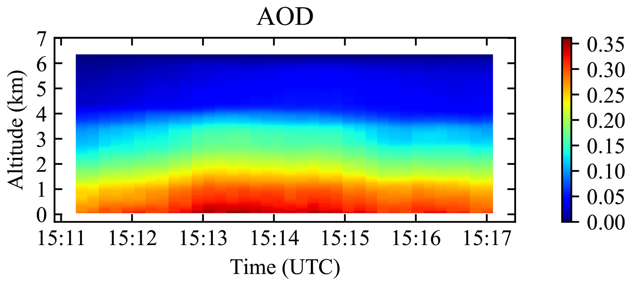
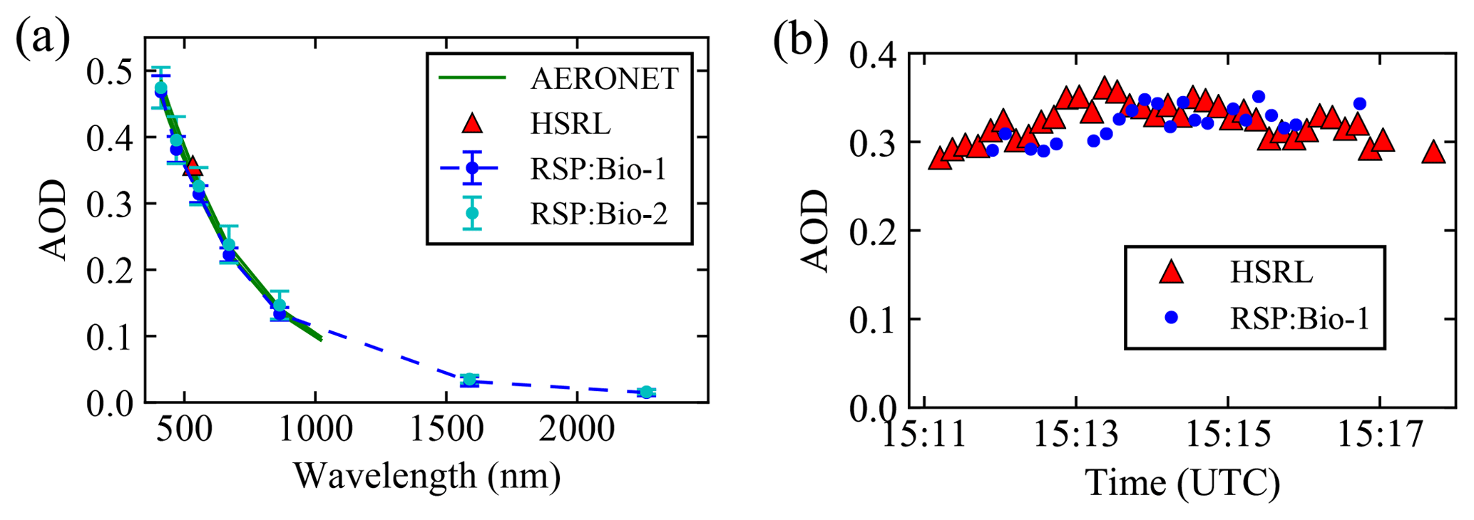
Figure 9(a) The comparison of the RSP-retrieved AOD, the HSRL AOD, and the AOD from AERONET site (COVE_SEAPRISM) for SABOR-Coastal. The error bars indicate the retrieval uncertainties. (b) The comparison of the RSP-retrieved AOD at 550 nm with the HSRL AOD across the flight track.
The vertical profile of HSRL AOD along the flight track is shown in Fig. 8, which indicates a small variation of the AOD and no apparent influence from clouds. Figure 9 shows that both bio-optical models can achieve accurate AOD retrieval as compared with the HSRL AOD and the AOD spectrum from the nearby AERONET site (COVE_SEAPRISM) with a distance of about 9.4 km. The COVE_SEAPRISM site measures AOD through the direct sunlight extinction from a Cimel sun-photometer-based system, called the Sea-Viewing Wide Field-of-View Sensor (SeaWiFS) Photometer Revision for Incident Surface Measurements (SeaPRISM), at eight wavelengths of 412, 443, 490, 532, 551, 667, 870, and 1020 nm (Zibordi et al., 2009). At a wavelength of 550 nm, RSP retrievals using Bio-1 obtain , while the retrievals using Bio-2 produce . The RSP AOD at 550 nm retrieved from both Bio-1 and Bio-2 is comparable with the HSRL AOD of 0.340. Although the RSP measurements are over coastal waters, the results using Bio-1 have a smaller uncertainties compared with Bio-2, probably resulting from the use of fewer retrieval parameters. The seven-parameter bio-optical model may be unnecessary in this case due to the small water-leaving signal and the large aerosol contribution. In the NAAMES-Coastal case that we will discuss later, Bio-2 has to be employed to achieve convergence because the water-leaving signal is strong and the aerosol contribution is weak. Figure 9b shows the RSP AOD retrieval with Bio-1 agrees well with the HSRL AOD along the track with . When using Bio-2, there are fewer retrieval results to reach the similar cost function level (data not shown) for the same set of initial values.
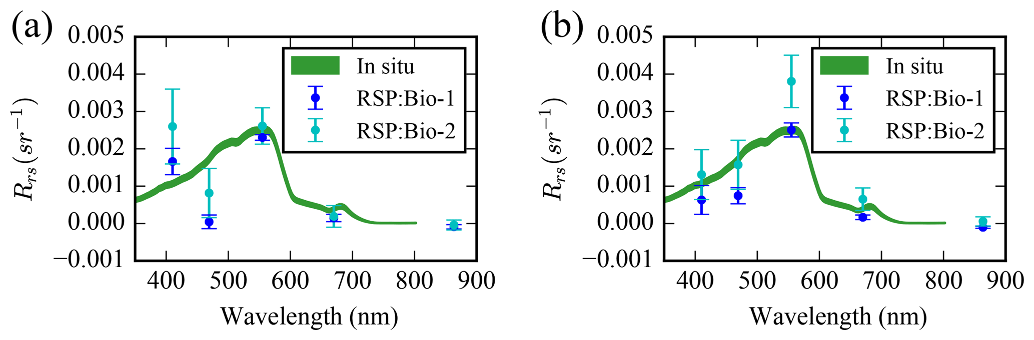
Figure 10(a) The comparison of the remote sensing reflectance from the RSP retrieval and the in situ measurement using two bio-optical models: Bio-1 and Bio-2. (b) Same as (a) but with extra retrieval parameters which adjust both the real and imaginary parts of the fine-mode refractive index at 410 nm and 470 nm. The vertical line width indicates the uncertainties of the in situ measurements, while the error bars indicate the retrieval uncertainties.
The retrieved remote sensing reflectance is compared with the in situ measurements from HyperPro, which is 1.7 km away from RSP measurements for the SABOR-Coastal case. The retrieved Rrs shares a similar spectral shape for the two bio-optical models, but with different uncertainties as shown in Fig. 10a. For example, Bio-1 retrieves Rrs at 410 nm with a value of 0.0017±0.00035, while Bio-2 obtains Rrs at 410 nm with a value of 0.0026±0.001, but both overestimate the in situ measurement value of 0.0010. At 470 nm, both retrievals underestimate the in situ measurement, with Bio-2 slightly closer to the in situ observations. For the wavelength at 550 nm Rrs is more accurately retrieved with uncertainties smaller than 1.0−4. The difference in the Rrs retrieval compared with the in situ measurement may be due to the small magnitude of the water-leaving signals and the large aerosol loadings.
Furthermore, there may be small variations in the aerosol refractive index spectrum that are not captured by the smooth representation of the PCA, which may affect the retrieval of water-leaving radiance adversely. For example, organic carbon may introduce spectral dependency of light absorption (Kirchstetter et al., 2004) but is not considered in the datasets used for the PCA computation. To explore the possibility of achieving better water-leaving radiance retrieval by accounting for this variation, we conducted the retrieval again by adding four retrieval parameters as the perturbations to the real and imaginary parts of the PCA refractive indices at 410 and 470 nm. The perturbations of the real parts are within ±0.1 and those of the imaginary parts are within ±0.01. A better agreement of the spectral shape of the retrieved Rrs can be found for both bio-optical models as shown in Fig. 10b, which is due to the additional refractive index spectral perturbation. The retrieved aerosol volume density is dominated by the fine-mode aerosols with the mean values of the real refractive indices of 1.58, 1.55, and 1.51 at 410, 470, and 550 nm, which deviate from the PCA representation by 0.06, 0.04, and 0.003. Meanwhile, the mean values for the fine-mode imaginary refractive indices are 0.014, 0.021, and 0.011 at 410, 470, and 550 nm, which differ from the PCA representation by 0.006, 0.014, and 0.004. It should be noted that SABOR-Coastal is the only case which needs the adjustment of refractive index at deep blue wavelengths. A larger validation dataset is needed to determine the scope of scenes that need this refractive index adjustment, which is currently unavailable in the community.
4.3 NAAMES-Open waters (26 May 2016)
On 26 May during the NAAMES02 field campaign in 2016, the aircraft flew over an open water region that was free from clouds. In situ measurements of water-leaving radiance are available from the R/V Atlantis, though they are not well colocated with the RSP measurement (the distance between the RSP footprint and the nearest in situ measurement is about 100 km). Despite the rather larger distance, it is still useful to compare the RSP retrieval and in situ measurement, assuming that the spatial variation in water properties is minimal at such an open water, offshore site. The in situ water-leaving signal was acquired by the Compact Optical Profiling System (C-OPS) instrument, which measured the upwelling radiance (Lu) and the downwelling irradiance (Ed) as a function of depth (NASA SeaBASS webpage, 2019). The data were then extrapolated to just above water surface using Eq. (4) to compute the remote sensing reflectance. The in situ measurements were collected at 18 wavelengths: 320, 340, 380, 395, 412, 443, 465, 490, 510, 532, 555, 560, 625, 665, 670, 683, 710, and 780 nm, and the data are publicly available in NASA's SeaBASS.
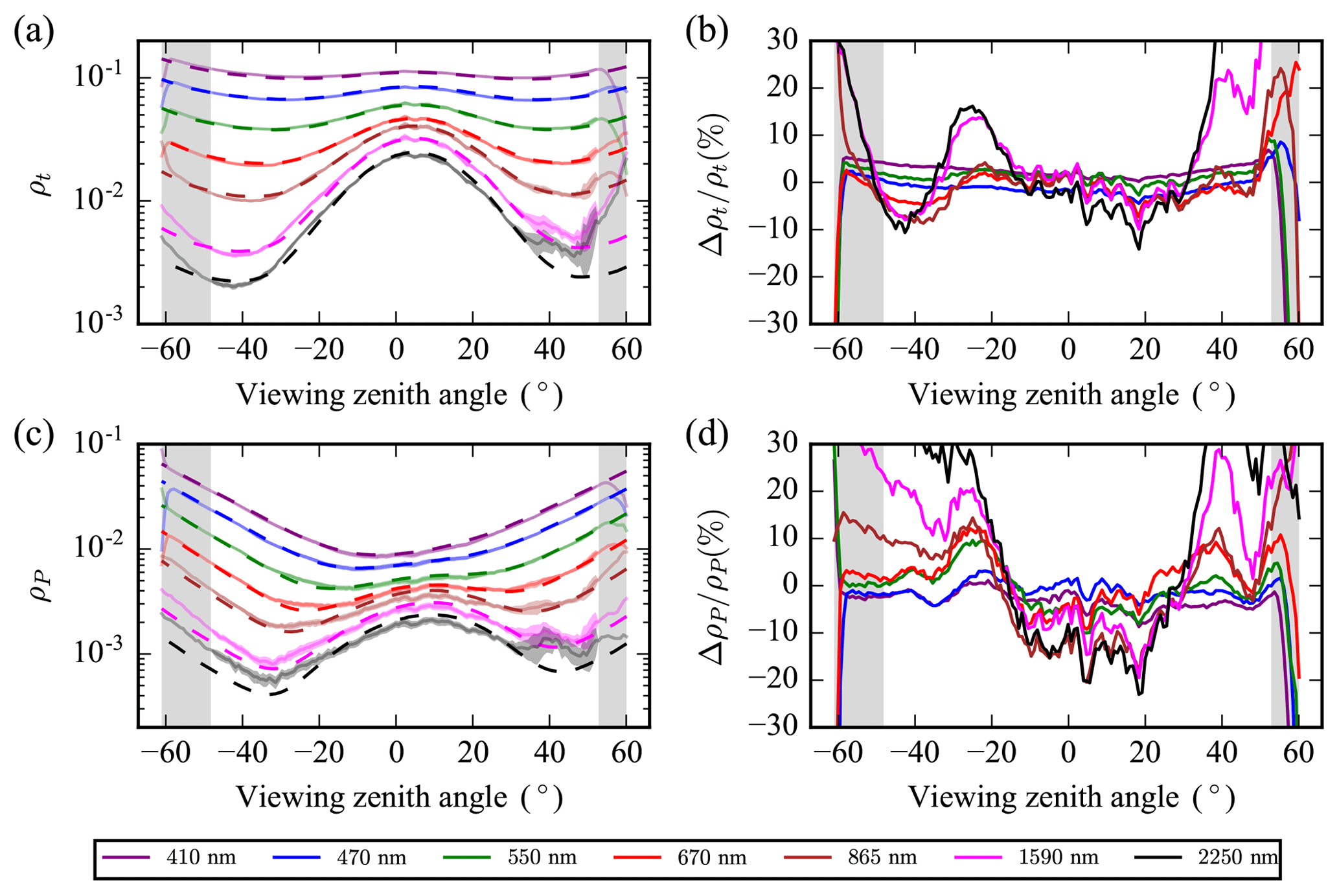
Figure 11Same as Fig. 3 but for NAAMES-Open on 26 May 2016. The minimum cost function value is and the bio-optical model used here is Bio-1.
As shown in Fig. 2c and Table 1, the RSP scanning direction for NAAMES-Open is almost perpendicular to the principle plane. However, with the solar zenith angle of 27∘, the RSP measurements contain prominent sunglint as shown in Fig. 11. The figure shows the best fitted simulation result with . Both the diffuse reflectance and sunglint have good agreement with the simulated reflectance ρt, with the percentage error generally less than 5 % for VIS bands, though larger errors approach 10 % in the NIR bands around the sunglint. There are errors even larger than 30 % for SWIR reflectance at viewing zenith angle greater than 30∘. For the polarized reflectance, the percentage difference is generally less than 10 % for VIS bands, but there are more prominent differences at both sides of sunglint especially for the SWIR bands.
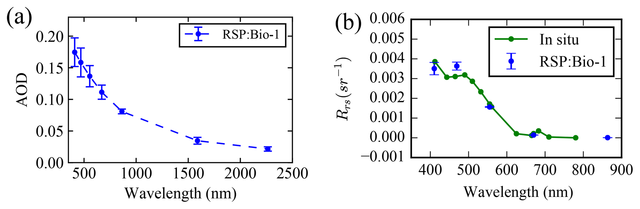
Figure 12(a) The RSP-retrieved AOD with uncertainties; (b) the comparison of the RSP-retrieved remote sensing reflectance with in situ measurement. The error bars indicate the retrieval uncertainties.
In order to discuss the retrieval uncertainties, a maximum cost function of is obtained. The retrieved optical depth at 550 nm is 0.137±0.017 as shown in Fig. 12a. The maximum uncertainties for AOD are at 410 nm with a value of 0.022, probably relating to the large AOD at the short wavelength. The remote sensing reflectance can be accurately determined with good agreement comparing with the in situ measurement as shown in Fig. 12b. The retrieval uncertainty for remote sensing reflectance at band 410 nm is 0.00031, which is larger than other bands.
The measurements at the SWIR bands at viewing angles between 30 and 50∘ show a peak with large uncertainties. These SWIR data lead to larger aerosol retrieval uncertainties; i.e., excluding the SWIR bands decreases the AOD uncertainties at 550 nm from 0.017 to 0.0084. The cost function decreases from 1.8 to 0.7 if the SWIR bands are excluded. However, excluding the SWIR bands in the retrieval slightly increases the retrieval uncertainty for Rrs at 410 nm from 0.00031 to 0.00041.
4.4 NAAMES-Coastal waters (4 November 2015)
On 4 November during the NAAMES01 campaign in 2015, the aircraft flew over the Delaware Bay where there are strong water-leaving signals and small aerosol loadings. Here, the choice of the bio-optical model is more important than for the SABOR-Coastal case, where the water-leaving signal is small. A location inside the Delaware Bay is chosen to discuss the retrieval uncertainties and the impact of the bio-optical models as shown in Fig. 1. Then, the retrieval over the whole flight track across the Delaware Bay is conducted and compared with the MODIS ocean color product. The RSP measurement was made at noon with the solar zenith angle near 60∘ as shown in Fig. 2d and in Table 1 for NAAMES-Coastal. The principal plane is almost perpendicular to the RSP scanning direction with a relative azimuth of 75∘. There is less influence from the sunglint as shown in Fig. 13. No RSP SWIR bands are available for this dataset.

Figure 13Same as Fig. 3 but for NAAMES-Coastal on 4 November 2015. The minimum cost function value is and the bio-optical model used here is Bio-2.
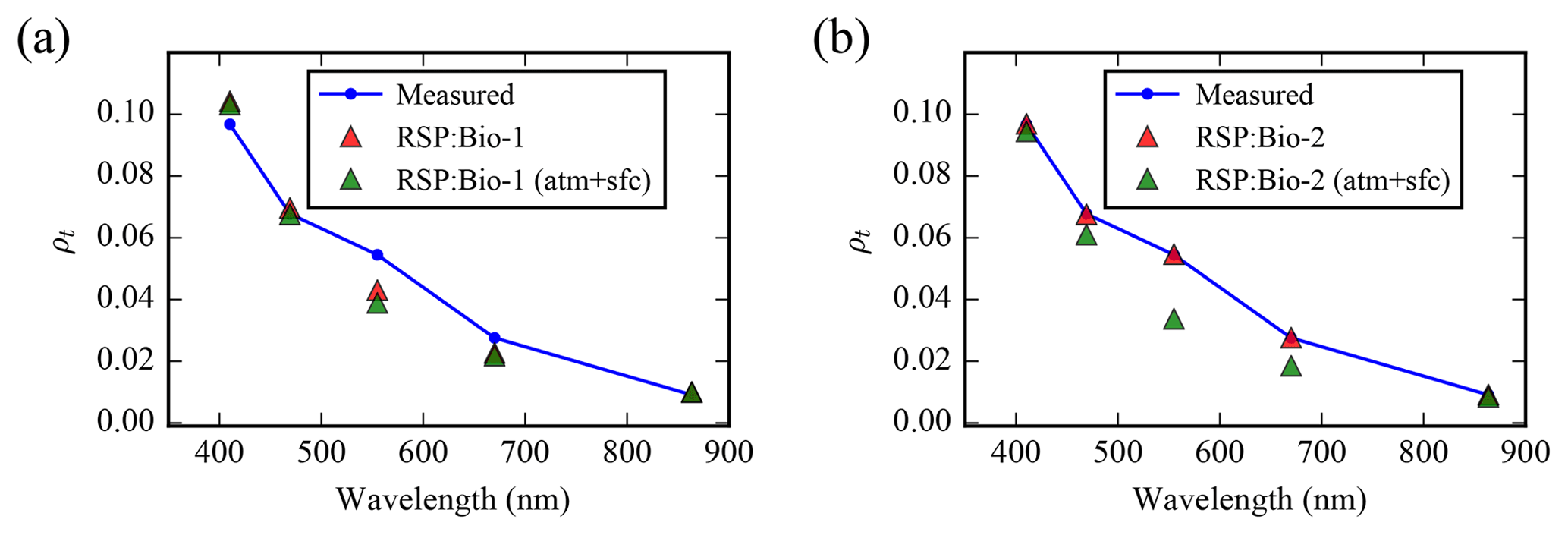
Figure 14The comparison of the measurement and the simulated total reflectance ρt of the whole atmosphere and ocean system, and the total reflectance from only the atmosphere and ocean surface (atm+sfc): (a) The RSP retrieval using Bio-1; (b) the RSP retrieval using Bio-2.
The maximum cost function value is with Bio-2 but increases to with Bio-1. The larger cost function value indicates a larger bias in the simulation. As we have discussed, Bio-1 works better for open water, as well as some coastal water cases when the water-leaving signal is small, such as the SABOR-Coastal case. As shown in Fig. 14a, for the retrieval using the Bio-1 model, the best fitted simulation result has a large minimum cost function of . The simulated reflectance tends to overestimate the reflectance at shorter wavelengths such as 410 nm and underestimate the reflectance at longer wavelengths at 550 and 670 nm. Consequently, a larger aerosol optical depth is retrieved as shown in Fig. 15a, and a negative remote sensing reflectance is obtained as shown in Fig. 15b. The reflectance with only the atmosphere and ocean surface (no ocean water body, denoted as “atm+sfc”) is also shown in Fig. 13. The difference between the total and the atm+sfc would be the contribution from the ocean water body only. When using the Bio-2 model, the comparison of the measured and best fitted simulation of ρt is shown in Fig. 14b. A good agreement can be found with difference less than 1 % at the nadir direction. The percentage difference for ρt over the whole viewing direction used in the retrieval is less than 2 % in ρt and less than 4 % for ρP as shown in Fig. 13b and d. Therefore, a smaller aerosol optical depth is retrieved as shown in Fig. 15a, and a more reasonable remote sensing reflectance spectrum is shown in Fig. 15b.
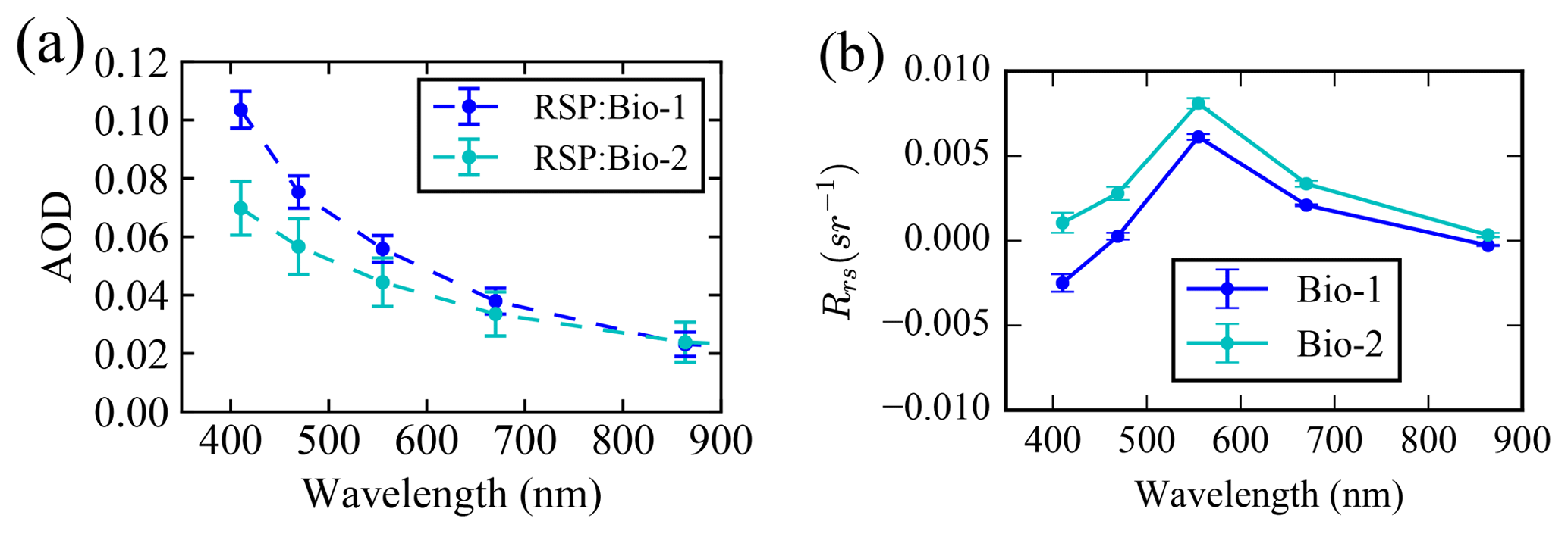
Figure 15(a) The comparison of the retrieved AOD using the two bio-optical models: Bio-1 and Bio-2; (b) same as (a) but for the remote sensing reflectance. The error bars indicate the retrieval uncertainties.
In this case, the maximum remote sensing reflectance is almost 3 times the maximum reflectance from the SABOR-Coastal case, thus requiring different consideration of the ocean signal through the bio-optical models in order to accurately conduct the retrieval algorithm for atmospheric correction. The retrieved optical depth and remote sensing reflectance strongly depend on the choice of the bio-optical models. When using Bio-1 and Bio-2, the retrieved AOD at 550 nm is 0.056±0.005 and respectively. Using Bio-1 results in a smaller variability in the AOD retrieval but much larger optical depths and negative remote sensing reflectances at shorter wavelength, suggesting that Bio-2 is necessary for this case. We use the averaged aerosol properties for the NAAMES-Coastal case as the initial values and conduct the joint retrieval along the whole flight track across the bay; the overall cost function is within χ2=1.35, which indicates good convergence along the track.
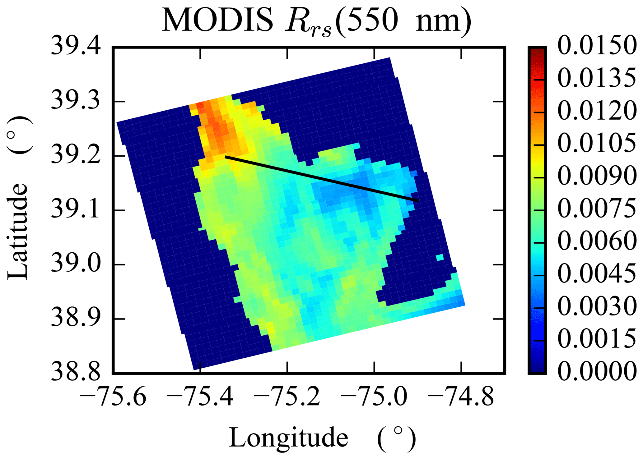
Figure 16The remote sensing reflectance for the 550 nm band from the MODIS ocean color product. The black line indicates the RSP flight track.
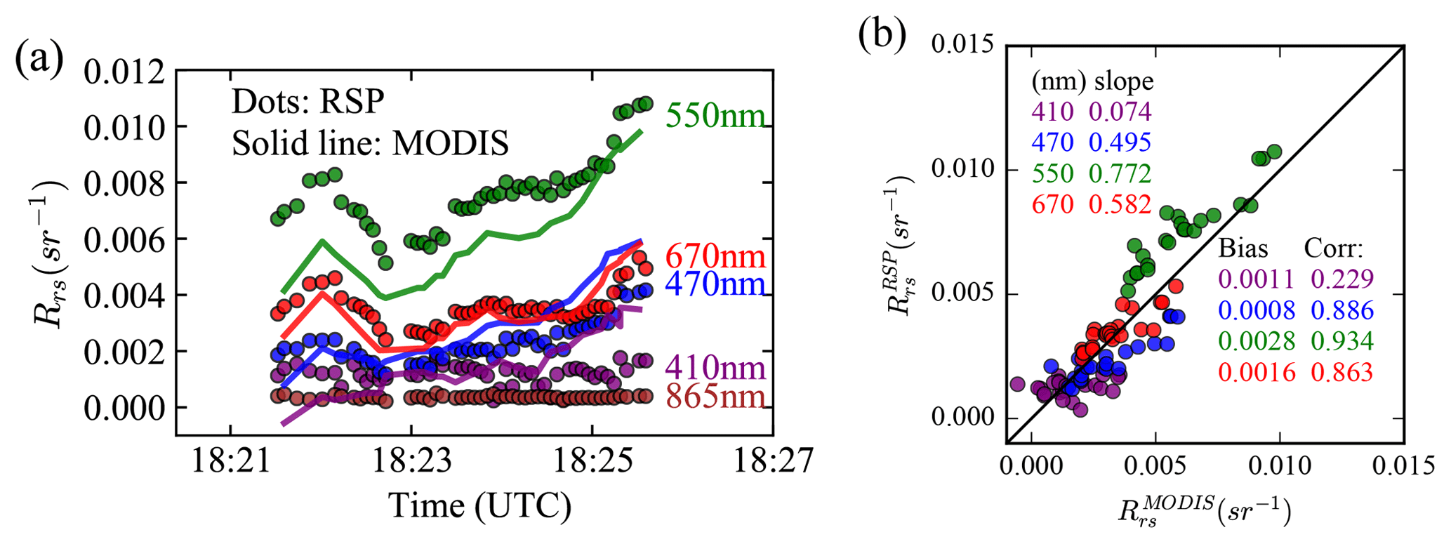
Figure 17(a) The comparison of the RSP-retrieved remote sensing reflectance across the Delaware Bay where dots indicate RSP retrieval and solid lines indicate the MODIS product. The time axis is from RSP measurement. (b) The correlation between the RSP and MODIS results with linear regression bias and slope shown for each wavelength.
The RSP-retrieved Rrs is compared with retrievals from MODIS/Aqua over the Delaware Bay. The MODIS ocean color product was generated by the SeaDAS l2gen software, which includes the atmospheric correction algorithm proposed by Gordon and Wang (1994) that is more recently described in its algorithm theoretical basis document (NASA Ocean Color Web, 2019). The MODIS ocean color product provides Rrs at 10 wavelengths: 412, 443, 469, 488, 531, 547, 555, 645, 667, and 678 nm. Figure 16 shows the RSP track in the MODIS Rrs image. The RSP pixels are collocated with the MODIS pixels within a distance of 500 m. The MODIS 412, 469, 555, and 667 nm bands are chosen to compare the corresponding RSP 410, 470, 550, and 670 nm bands. The Rrs from RSP and MODIS shows similar spatial variations in Fig. 17a. Figure 17b shows the correlation (corr) for each band with the linear regression slope and bias. The bands 470, 550, and 670 all show high correlation of 0.88, 0.93, and 0.86 respectively. The Rrs from RSP and MODIS agrees well for 670 nm across the whole track. We found RSP-retrieved Rrs values are larger than the MODIS retrievals with a value between 0.001 and 0.002 from 18:21 to 18:24 UTC at 550 nm, while they are smaller than the MODIS retrievals within a value within 0.001 from 18:24 to 18:26 UTC at 410 nm. On average, the mean absolute errors (MAEs) between the RSP and MODIS retrievals are 0.0009, 0.0009, 0.0015, and 0.0005 for the 410, 470, 550, and 670 nm bands, while the corresponding root mean square errors (RMSEs) are 0.0011, 0.0011, 0.0016, and 0.0006. The possible reason for the discrepancy may be due to the different aerosol model retrieved/selected for RSP and MODIS using two completely different algorithms and datasets. MODIS retrievals rely on two NIR bands of 748 and 869 nm to determine the aerosol model, while RSP retrievals conduct radiative transfer simulations for all VIS and NIR bands from 410 to 865 nm based on a coupled atmosphere and ocean model.
The uncertainties of the remote sensing reflectance retrievals associated with different initial values in the optimization are evaluated and summarized in Table 5 for wavelengths from 410 to 670 nm, where the SABOR-Coastal case with the Bio-1 model is excluded due to its large χ2 value in fitting the measurement as shown in Table 4. This uncertainty is due to the local minima of the cost function in the retrieval, which have not been quantified before for the study of atmospheric correction. Due to the large number of retrieval parameters and the nonlinearity of the cost functions, the choice of the initial values often becomes important, and it is essential to understand the corresponding uncertainty and also its relationship with the PACE requirement on atmospheric correction.
Table 5The atmospheric correction uncertainties for the four cases as listed in Table 1 for the RSP retrieval. The uncertainties are computed through using different initial values in the optimization. The PACE requirement for open ocean (values in the parenthesis) is shown. The numbers in bold indicate the RSP retrieval uncertainties larger than the PACE requirement. Bio-1 is the [Chl a]-based bio-optical model used for open waters, and Bio-2 is the generalized bio-optical model used for coastal waters. For the SABOR-Coastal case where the aerosol loading is larger and the water-leaving signal is small, both bio-optical models are computed for discussion. All cases use the seven RSP bands except for the one indicated by an asterisk which did not use SWIR bands.
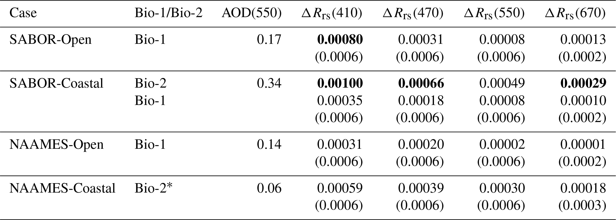
The PACE requirement on the atmospheric correction for open ocean is to retrieve the normalized water-leaving reflectance [ρw(λ)]N with an accuracy of the maximum of either 5 % or 0.002 over the spectral range of 400–600 nm and the maximum of either 10 % or 0.0007 over the spectral range of 600–710 nm (Werdell et al., 2019). Since the normalized water-leaving reflectance can be related to the remote sensing reflectance through [ρw(λ)]N=πRrs (Mobley et al., 2016), the PACE requirement on Rrs can be computed accordingly and compared with the RSP retrieval accuracy in Table 5.
For the open water cases, the retrieval uncertainty for the remote sensing reflectance is smaller than the PACE atmospheric correction requirement for all the bands except for 410 nm in the SABOR-Open case, where the retrieval uncertainty is 0.0008 larger than the PACE requirement of 0.0006. For NAAMES-Open, the maximum retrieval uncertainty for Rrs at 410 nm is 0.00031, which is smaller than the PACE requirement of 0.0006.
For coastal waters, it is more challenging to retrieve the remote sensing reflectance accurately due to the complex water properties. Since the PACE atmospheric correction for coastal waters is not available, we use the same PACE requirement for open water in comparison. The two bio-optical models are applied in the coastal water cases; for the NAAMES-Coastal case, only Bio-2 provided a reasonable result, while Bio-1 causes a negative value of Rrs at shorter wavelengths. The maximum retrieval uncertainty at 410 nm with a value of 0.00059 is close to the PACE requirement of 0.0006 as shown in Table 4. All the other bands are well within the requirement. In this coastal water case, the water-leaving signal is strong, and it is therefore important to select the bio-optical model to provide proper constraints of the water-leaving signal in the coupled atmosphere and ocean system.
For the SABOR-Coastal case, due to the large aerosol loading and small water-leaving signals, both bio-optical models demonstrated comparable results in aerosol and water-leaving signal retrievals. Due to the larger number of retrieval parameters for Bio-2, the retrieval uncertainties are larger, with values of 0.001, 0.00066, 0.00049, and 0.00029 at 410, 470, 550, and 670 nm respectively, where the uncertainties at 410, 470, and 670 nm are larger than the PACE requirement of 0.0006, 0.0006 and 0.0002. When using Bio-1, the retrieval uncertainties are much reduced with the maximum uncertainty of 0.00035 at band 410 nm smaller than the PACE requirement. Meanwhile, both bio-optical models result in high accuracy in the retrieval of the AOD as compared with the AERONET and HSRL AOD product. Furthermore, two treatments of the refractive index spectra are compared in the retrieval for the SABOR-Coastal case. When using the PCA representation of aerosol refractive indices, there is a dip at 470 nm in the spectra shape of the retrieved remote sensing reflectance, which is different from the in situ measurement. This suggest that the aerosol refractive index spectrum may have small spectral variation which is not captured by the current representation of PCA. After introducing a small adjustment of the refractive index at the 410 and 470 nm bands in the retrieval, the retrieved remote sensing reflectance resembles a similar shape compared to the in situ measurement. Both treatments of the refractive index carry similar uncertainties. If additional collocated datasets are available for validation in the future, we will further investigate and attempt to identify the best representation of the refractive index spectrum beyond PCA with better flexibility and stability.
The MAPOL retrieval algorithm provides accurate retrieval of the aerosol properties as compared with the HSRL and AERONET AOD over both open and coastal waters. The remote sensing reflectance can also be accurately retrieved as compared with the in situ measurements. Meanwhile, the measurement dataset needs to be carefully examined to remove all the possible influence from cloud and other error sources. The retrieval with the measurement over sunglint also requires close examination where the sunglint may be influenced by wind direction or instantaneous ocean surface slopes with large waves that are not described in the forward model. Overall the retrieval uncertainties are comparable with the PACE atmospheric correction requirement, and higher uncertainties are mostly associated with the deep blue 410 nm band.
The retrieval uncertainties associated with the local minimum can help to determine better initial values and quantify the accuracy. The uncertainties from the error propagation of the instrument noise can also be evaluated with the selected initial value and provide another aspect of the retrieval uncertainties (Rogers, 2000). The joint retrieval algorithm will be applied to HARP2 and SPEXone to evaluate the possible accuracy directly relevant to the PACE mission.
We have developed a joint retrieval algorithm (MAPOL) for aerosol and water-leaving properties based on a radiative transfer model for coupled atmosphere and ocean systems. Both the aerosol optical properties and ocean bio-optical properties are flexible in order to model complex coastal scenes. The algorithm has been validated for synthetic measurements in a previous study. In this study, we applied the MAPOL retrieval algorithm to RSP airborne measurements. Four cases from the SABOR and NAAMES field campaigns are chosen with two open and two coastal water cases. Our retrieval results indicate a good agreement in the aerosol optical depth compared with both the HSRL and AERONET products, as well as a good agreement of the remote sensing reflectance as compared with in situ measurements and the MODIS ocean color products.
Two different but related bio-optical models are implemented and discussed in the retrieval algorithm for the study of atmospheric correction over different water conditions. For open waters, the [Chl a]-based bio-optical model (Bio-1) is used with a single parameter to define all seawater components, while for coastal waters, a seven-parameter bio-optical model (Bio-2) is employed. To understand the applicability of the two bio-optical models, both models are applied in the coastal waters cases from SABOR and NAAMES. For the SABOR coastal water cases, the water-leaving signal is weak and both bio-optical models provide similar results of aerosol and the remote sensing reflectance retrieval, but there is a smaller uncertainty associated with Bio-1. For the NAAMES coastal waters, the water-leaving signal is relatively strong, and only Bio-2 can provide a reasonable remote sensing reflectance retrieval that avoids negative values.
Using RSP retrievals in open waters as a proxy, we show that this joint retrieval can nearly meet PACE mission requirements for atmospheric correction at shorter wavelengths (e.g., 410 nm) and performs well within the requirement at longer wavelengths. For coastal waters, the appropriate bio-optical model may be selected depending on the magnitude of the water-leaving signal and the uncertainty requirement. Generally, Bio-2 may have larger uncertainties compared with Bio-1 due to its larger parameter space, but it is necessary to use Bio-2 in order to better fit the data and avoid negative reflectance retrievals for certain cases. A comparison with the MODIS ocean color product shows high correlation but also differences in magnitudes in remote sensing reflectances.
The cases we studied cover various aerosol loadings, viewing geometry, and sunglint conditions, providing a useful quantification for the retrieval uncertainties of both aerosol and water-leaving signals in the study of atmospheric correction using the multiangle, multiwavelength, and polarization measurements. It provides a useful understanding to better harvest the rich information in such measurements and to reduce the possible influence from various error sources such as clouds and sunglint. The MAPOL algorithm provides a flexible description of the aerosol and ocean bio-optical properties, and when combined with more colocated remote sensing reflectances and in situ measurement, a more efficient algorithm may be developed to reduce and optimize the retrieval parameters in the algorithm. The lessons discussed and the accuracy evaluated from the retrieval with the polarization measurement for atmospheric correction can assist the future development of the atmospheric correction algorithm for the PACE mission, with the goal of combining both the OCI and polarimeter measurements.
As shown in Table 1 and Fig. 1, four cases from the RSP measurements are studied from both the SABOR and NAAMES campaigns. The corresponding RSP L1B data can be located from the NASA GISS website (NASA RSP Data Site, 2019). The file names are listed as follows.
-
SABOR-Open (27 July 2014):
RSP1-UC12_L1B-RSPGEOL1B-GeolocatedRadiances_20140727T141100Z_V001-20160518T201607Z.h5. -
SABOR-Coastal (30 July 2014):
RSP1-UC12_L1B-RSPGEOL1B-GeolocatedRadiances_20140730T151114Z_V001-20160518T213810Z.h5. -
NAAMES-Open (26 May 2016):
RSP1-C130_L1B-RSPGEOL1B-GeolocatedRadiances_20160526T150519Z_V001-20160601T174243Z.h5. -
NAAMES-Coastal (4 November 2015):
RSP1-C130_L1B-RSPGEOL1B-GeolocatedRadiances_20151104T182047Z_V002-20161129T190435Z.h5.
The remote sensing reflectance defined in this study is represented in Eq. (2) as
where td is the downward transmittance of the solar irradiance to the surface, and tu is the upward transmittance of the water-leaving radiance to the detector. To compute the remote sensing reflectance quantitatively, can be obtained from the difference between the measurement ρt and the simulated reflectance at the sensor considering only the atmosphere and ocean surface (denoted by atm+sfc following the notation by Gao et al., 2000)
Both td and tu are due to the scattering and absorption in the atmosphere and can be computed from the radiative transfer simulation. Specifically, the transmittance td is defined as the ratio of downwelling irradiance just above the ocean surface with respect to the solar irradiance F0 as
where is computed from the forward model using the retrieved atmosphere properties. tu is the transmittance of the upwelling water-leaving radiance from surface to the sensor at certain viewing direction θv, which can be estimated as
where all the quantities are computed from the forward model, represents the total radiance at the sensor, and represents the radiance just above the ocean surface computed from the forward model with the total atmosphere and ocean system; same for and but considering only the atmosphere and ocean surface with no scattering in the ocean. Therefore represents the water-leaving radiance just above the ocean surface, and represents the water-leaving radiance which transmits to the sensor. Note that since the water-leaving reflectance is generally small, we ignored the contribution from the reflection of the water-leaving signals by the atmosphere back to the ocean.
The RSP uncertainty model used in this study is summarized as follows. More details are in Knobelspiesse et al. (2019). The error covariance and for radiance and polarized radiance in Eq. (3) are defined as the sum of noise and calibration uncertainties:
The same is true for the total uncertainty of the polarized reflectance uncertainty model:
Two RSP instruments have been built with name RSP1 and RSP2. In our study, the measurement are only from RSP1, with noises and uncertainties including detector floor noise , shot noise parameter , relative gain coefficient characterization uncertainty σln K=0.005, absolute radiometric characterization uncertainty , and polarimetric characterization uncertainty σln α=0.002. Solar distance (r) is in astronomical units with a value of 1.0. RSP2 has a slightly different noise model which is not discussed here.
The [Chl a]-based bio-optical model (Bio-1) can be derived from the generalized bio-optical model (Bio-2) by imposing constraints on its parameters for the study of open waters (Zhai et al., 2015, 2017). The phytoplankton absorption coefficient aph is the same as in Table 3. Since no contribution from NAP is assumed for open waters, the particulate absorption coefficient adg depends only on phytoplankton. Its parameter adg(440) is specified by [Chl a] as
where R2=0.5 is assumed and a fixed value of Sdg=0.018 is used.
The particulate scattering coefficients bbp also depends only on phytoplankton for open water studies. Its parameter bbp(660) is specified by [Chl a] as
The spectral slope is specified as for mg m−3, otherwise zero. The particulate backscattering fraction can be specified as where Bp is assumed to be spectrally flat (Huot et al., 2008).
MG and PWZ developed the retrieval algorithm and generated the scientific data used in this paper. MG wrote the original manuscript. PWZ and BF formulated the original concept for this study. KK advised on the RSP noise model. BC advised on the use of RSP data and the retrieval sensitivity of aerosols. PJW, AI, and YH advised on the ocean bio-optical models. AC provided and analyzed the HyperPro measurement data. All authors participated the writing and editing of this paper.
The authors declare that they have no conflict of interest.
Yongxiang Hu was funded by the NASA Radiation Science Program administrated by Hal Maring and the Biology and Biogeochemistry program administrated by Paula Bontempi. The authors would like to thank the NAAMES and SABOR teams, including the crew and captains of R/V Endeavor and R/V Atlantis, as well as the NASA AERONET team and the NASA Langley team for maintaining the AERONET COVE_SEAPRISM site. The authors also thank the two anonymous reviewers for their constructive comments.
The hardware used in the computational studies is part of the UMBC High Performance Computing Facility (HPCF). The facility is supported by the U.S. National Science Foundation through the MRI program (grant nos. CNS-0821258, CNS-1228778, and OAC-1726023) and the SCREMS program (grant no. DMS-0821311), with additional substantial support from the University of Maryland, Baltimore County (UMBC). See https://hpcf.umbc.edu/ (last access: 1 July 2019) for more information on HPCF and the projects using its resources.
This research has been supported by the National Aeronautics and Space Administration (grant no. 80NSSC18K0345) and the National Aeronautics and Space Administration (grant no. NNX15AK87G).
This paper was edited by Alexander Kokhanovsky and reviewed by two anonymous referees.
Bricaud, A., Morel, A., Babin, M., Allali, K., and Claustre, H.: Variations of light absorption by suspended particles with chlorophyll a concentration in oceanic (case 1) waters: Analysis and implications for bio-optical models, J. Geophys. Res.-Oceans, 103, 31033–31044, 1998. a
Cairns, B., Russell, E. E., and Travis, L. D.: Research Scanning Polarimeter: calibration and ground-based measurements, Proc. SPIE, 3754, 11, https://doi.org/10.1117/12.366329, 1999. a, b
Chapman, D. V.: Water quality assessments: a guide to the use of biota, sediments and water in environmental monitoring, 2nd edn., E & FN Spon, published on behalf of United Nations Educational, Scientific and Cultural Organization, World Health Organization, United Nations Enviroment Programme, London, 1996 a
Chase, A. P., Boss, E., Cetinić, I., and Slade, W.: Estimation of Phytoplankton Accessory Pigments From Hyperspectral Reflectance Spectra: Toward a Global Algorithm, J. Geophys. Res.-Oceans, 122, 9725–9743, 2017. a
Chowdhary, J., Cairns, B., Mishchenko, M. I., Hobbs, P. V., Cota, G. F., Redemann, J., Rutledge, K., Holben, B. N., and Russell, E.: Retrieval of Aerosol Scattering and Absorption Properties from Photopolarimetric Observations over the Ocean during the CLAMS Experiment, J. Atmos. Sci., 62, 1093–1117, https://doi.org/10.1175/JAS3389.1, 2005. a, b, c
Chowdhary, J., Cairns, B., Waquet, F., Knobelspiesse, K., Ottaviani, M., Redemann, J., Travis, L., and Mishchenko, M.: Sensitivity of multiangle, multispectral polarimetric remote sensing over open oceans to water-leaving radiance: Analyses of RSP data acquired during the MILAGRO campaign, Remote Sens. Environ., 118, 284–308, 2012. a, b, c
Costanza, R.: The ecological, economic, and social importance of the oceans, Ecol. Econ., 31, 199–213, https://doi.org/10.1016/S0921-8009(99)00079-8, 1999. a
Cox, C. and Munk, W.: Measurement of the Roughness of the Sea Surface from Photographs of the Sun's Glitter, J. Opt. Soc. Am., 44, 838–850, 1954. a
d'Almeida, G. A., Koepke, P., and Shettle, E. P.: Atmospheric aerosols: global climatology and radiative characteristics, A Deepak Pub, Hampton, 1991. a
Dubovik, O., Herman, M., Holdak, A., Lapyonok, T., Tanré, D., Deuzé, J. L., Ducos, F., Sinyuk, A., and Lopatin, A.: Statistically optimized inversion algorithm for enhanced retrieval of aerosol properties from spectral multi-angle polarimetric satellite observations, Atmos. Meas. Tech., 4, 975–1018, https://doi.org/10.5194/amt-4-975-2011, 2011. a
Dubovik, O., Li, Z., Mishchenko, M. I., Tanré, D., Karol, Y., Bojkov, B., Cairns, B., Diner, D. J., Espinosa, W. R., Goloub, P., Gu, X., Hasekamp, O., Hong, J., Hou, W., Knobelspiesse, K. D., Landgraf, J., Li, L., Litvinov, P., Liu, Y., Lopatin, A., Marbach, T., Maring, H., Martins, V., Meijer, Y., Milinevsky, G., Mukai, S., Parol, F., Qiao, Y., Remer, L., Rietjens, J., Sano, I., Stammes, P., Stamnes, S., Sun, X., Tabary, P., Travis, L. D., Waquet, F., Xu, F., Yan, C., and Yin, D.: Polarimetric remote sensing of atmospheric aerosols: Instruments, methodologies, results, and perspectives, J. Quant. Spectrosc. Ra., 224, 474–511, https://doi.org/10.1016/j.jqsrt.2018.11.024, 2019. a
Fournier, G. R. and Forand, J. L.: Analytic phase function for ocean water, Proc. SPIE, 2258, 8, https://doi.org/10.1117/12.190063, 1994. a, b
Gao, B.-C., Montes, M. J., Ahmad, Z., and Davis, C. O.: Atmospheric correction algorithm for hyperspectral remote sensing of ocean color from space, Appl. Opt., 39, 887–896, https://doi.org/10.1364/AO.39.000887, 2000. a, b
Gao, M., Zhai, P.-W., Franz, B., Hu, Y., Knobelspiesse, K., Werdell, P. J., Ibrahim, A., Xu, F., and Cairns, B.: Retrieval of aerosol properties and water-leaving reflectance from multi-angular polarimetric measurements over coastal waters, Opt. Express, 26, 8968–8989, https://doi.org/10.1364/OE.26.008968, 2018. a, b, c, d, e, f, g, h, i
Gordon, H. R. and Wang, M.: Retrieval of water-leaving radiance and aerosol optical thickness over the oceans with SeaWiFS: a preliminary algorithm, Appl. Opt., 33, 443–452, 1994. a
Hair, J. W., Hostetler, C. A., Cook, A. L., Harper, D. B., Ferrare, R. A., Mack, T. L., Welch, W., Izquierdo, L. R., and Hovis, F. E.: Airborne High Spectral Resolution Lidar for profiling aerosol optical properties, Appl. Opt., 47, 6734–6752, https://doi.org/10.1364/AO.47.006734, 2008. a
Hasekamp, O. P., Litvinov, P., and Butz, A.: Aerosol properties over the ocean from PARASOL multiangle photopolarimetric measurements, J. Geophys. Res.-Oceans, 116, D14204, 2011. a, b, c
Hasekamp, O. P., Fu, G., Rusli, S. P., Wu, L., Noia, A. D., aan de Brugh, J., Landgraf, J., Smit, J. M., Rietjens, J., and van Amerongen, A.: Aerosol measurements by SPEXone on the NASA PACE mission: expected retrieval capabilities, J. Quant. Spectrosc. Ra., 227, 170–184, https://doi.org/10.1016/j.jqsrt.2019.02.006, 2019. a
Holben, B., Eck, T., Slutsker, I., Tanré, D., Buis, J., Setzer, A., Vermote, E., Reagan, J., Kaufman, Y., Nakajima, T., Lavenu, F., Jankowiak, I., and Smirnov, A.: AERONET—A Federated Instrument Network and Data Archive for Aerosol Characterization, Remote Sens. Environ., 66, 1–16, https://doi.org/10.1016/S0034-4257(98)00031-5, 1998. a
Huot, Y., Morel, A., Twardowski, M. S., Stramski, D., and Reynolds, R. A.: Particle optical backscattering along a chlorophyll gradient in the upper layer of the eastern South Pacific Ocean, Biogeosciences, 5, 495–507, https://doi.org/10.5194/bg-5-495-2008, 2008. a
Jamet, C., Ibrahim, A., Ahmad, Z., Angelini, F., Babin, M., Behrenfeld, M. J., Boss, E., Cairns, B., Churnside, J., Chowdhary, J., Davis, A. B., Dionisi, D., Duforêt-Gaurier, L., Franz, B., Frouin, R., Gao, M., Gray, D., Hasekamp, O., He, X., Hostetler, C., Kalashnikova, O. V., Knobelspiesse, K., Lacour, L., Loisel, H., Martins, V., Rehm, E., Remer, L., Sanhaj, I., Stamnes, K., Stamnes, S., Victori, S., Werdell, J., and Zhai, P.-W.: Going Beyond Standard Ocean Color Observations: Lidar and Polarimetry, Front. Mar. Sci., 6, 251, https://doi.org/10.3389/fmars.2019.00251, 2019. a
Kirchstetter, T. W., Novakov, T., and Hobbs, P. V.: Evidence that the spectral dependence of light absorption by aerosols is affected by organic carbon, J. Geophys. Res.-Atmos., 109, D21208, https://doi.org/10.1029/2004JD004999, 2004. a
Knobelspiesse, K., Cairns, B., Mishchenko, M., Chowdhary, J., Tsigaridis, K., van Diedenhoven, B., Martin, W., Ottaviani, M., and Alexandrov, M.: Analysis of fine-mode aerosol retrieval capabilities by different passive remote sensing instrument designs, Opt. Express, 20, 21457–21484, https://doi.org/10.1364/OE.20.021457, 2012. a, b
Knobelspiesse, K., Tan, Q., Bruegge, C., Cairns, B., Chowdhary, J., van Diedenhoven, B., Diner, D., Ferrare, R., van Harten, G., Jovanovic, V., Ottaviani, M., Redemann, J., Seidel, F., and Sinclair, K.: Intercomparison of airborne multi-angle polarimeter observations from the Polarimeter Definition Experiment, Appl. Opt., 58, 650–669, https://doi.org/10.1364/AO.58.000650, 2019. a, b, c, d
Kokhanovsky, A. A.: Parameterization of the Mueller matrix of oceanic waters, J. Geophys. Res.-Oceans, 108, 3175, 2003. a
Kou, L., Labrie, D., and Chylek, P.: Refractive indices of water and ice in the 0.65- to 2.5-µm spectral range, Appl. Opt., 32, 3531–3540, 1993. a, b
Kuchinke, C. P., Gordon, H. R., and Franz, B. A.: Spectral optimization for constituent retrieval in Case 2 waters I: Implementation and performance, Remote Sens. Environ., 113, 571–587, https://doi.org/10.1016/j.rse.2008.11.001, 2009. a
Martins, J. V., Nielsen, T., Fish, C., Sparr, L., Fernandez-Borda, R., Schoeberl, M., and Remer, L.: HARP CubeSat –- An innovative Hyperangular Imaging Polarimeter for Earth Science Applications, Small Sat Pre-Conference Workshop, Logan Utah, 2014. a
Mobley, C. D.: Light and Water: Radiative Transfer in Natural Waters, Academic Press, San Diego, 1994. a, b, c, d
Mobley, C. D., Werdell, J., Franz, B., Ahmad, Z., and Bailey, S.: Atmospheric Correction for Satellite Ocean Color Radiometry, National Aeronautics and Space Administration, Greenbelt, Maryland, USA, 2016. a, b
Moré, J. J.: The Levenberg-Marquardt algorithm: Implementation and theory, in: Numerical Analysis, edited by: Watson, G. A., Springer Berlin Heidelberg, Berlin, Heidelberg, 1978. a
Moré, J. J., Garbow, B., and Hillstrom, K.: User guide for MINPACK-1, Argonne National Laboratory Report ANL-80-74, Argonne, Ill, 1980. a
NASA NAAMES webpage: available at: https://naames.larc.nasa.gov/ (last access: 1 July 2019), 2019. a
NASA Ocean Color Web: available at: https://oceancolor.gsfc.nasa.gov/atbd/rrs/ (last access: 1 July 2019), 2019. a
NASA RSP Data Site: available at: https://data.giss.nasa.gov/pub/rsp (last access: 1 July 2019), 2019. a
NASA SABOR webpage: available at: https://espo.nasa.gov/sabor/content/SABOR (last access: 1 July 2019), 2019. a
NASA SeaBASS webpage: available at: https://seabass.gsfc.nasa.gov/ (last access: 1 July 2019), 2019. a, b
National Academies of Sciences, Engineering, and Medicine: Thriving on Our Changing Planet: A Decadal Strategy for Earth Observation from Space, The National Academies Press, Washington, DC, https://doi.org/10.17226/24938, 2018. a
Ottaviani, M., Foster, R., Gilerson, A., Ibrahim, A., Carrizo, C., El-Habashi, A., Cairns, B., Chowdhary, J., Hostetler, C., Hair, J., Burton, S., Hu, Y., Twardowski, M., Stockley, N., Gray, D., Slade, W., and Cetinic, I.: Airborne and shipborne polarimetric measurements over open ocean and coastal waters: Intercomparisons and implications for spaceborne observations, Remote Sens. Environ., 206, 375–390, https://doi.org/10.1016/j.rse.2017.12.015, 2018. a
Pope, R. M. and Fry, E. S.: Absorption spectrum (380–700 nm) of pure water, II, Integrating cavity measurements, Appl. Opt., 36, 8710–8723, 1997. a, b
Rogers, C.: Inverse Methods for Atmospheric Sounding: Theory and Practice, World Scientific World Scientific Publishing, Singapore, 2000. a, b, c
Sathyendranath, S. (Ed.): Remote sensing of ocean colour in coastal, and other optically-complex, waters, International Ocean Colour Coordinating Group (IOCCG), 2000. a
Shettle, E. P. and Fenn, R. W.: Models for the aerosols of the lower atmosphere and the effects of humidity variations on their optical properties, Environmental Research Papers, Air Force Geophysics Lab., Hanscom AFB, MA. Optical Physics Div, 1979. a
Stamnes, S., Hostetler, C., Ferrare, R., Burton, S., Liu, X., Hair, J., Hu, Y., Wasilewski, A., Martin, W., van Diedenhoven, B., Chowdhary, J., Cetinić, I., Berg, L. K., Stamnes, K., and Cairns, B.: Simultaneous polarimeter retrievals of microphysical aerosol and ocean color parameters from the “MAPP” algorithm with comparison to high-spectral-resolution lidar aerosol and ocean products, Appl. Opt., 57, 2394–2413, https://doi.org/10.1364/AO.57.002394, 2018. a, b, c
Stap, F. A., Hasekamp, O. P., and Röckmann, T.: Sensitivity of PARASOL multi-angle photopolarimetric aerosol retrievals to cloud contamination, Atmos. Meas. Tech., 8, 1287–1301, https://doi.org/10.5194/amt-8-1287-2015, 2015. a
Voss, K. J. and Fry, E. S.: Measurement of the Mueller matrix for ocean water, Appl. Opt., 23, 4427–4439, 1984. a
Wang, M. (Ed.): Atmospheric Correction for Remotely-Sensed Ocean-Colour, International Ocean Colour Coordinating Group (IOCCG), 2010. a
Werdell, P. J., Behrenfeld, M. J., Bontempi, P. S., Boss, E., Cairns, B., Davis, G. T., Franz, B. A., Gliese, U. B., Gorman, E. T., Hasekamp, O., Knobelspiesse, K. D., Mannino, A., Martins, J. V., McClain, C. R., Meister, G., and Remer, L. A.: The Plankton, Aerosol, Cloud, ocean Ecosystem (PACE) mission: Status, science, advances, B. Am. Meteorol. Soc., in press, https://doi.org/10.1175/BAMS-D-18-0056.1, 2019. a, b
Wu, L., Hasekamp, O., van Diedenhoven, B., and Cairns, B.: Aerosol retrieval from multiangle, multispectral photopolarimetric measurements: importance of spectral range and angular resolution, Atmos. Meas. Tech., 8, 2625–2638, https://doi.org/10.5194/amt-8-2625-2015, 2015. a
Xu, F., Dubovik, O., Zhai, P.-W., Diner, D. J., Kalashnikova, O. V., Seidel, F. C., Litvinov, P., Bovchaliuk, A., Garay, M. J., van Harten, G., and Davis, A. B.: Joint retrieval of aerosol and water-leaving radiance from multispectral, multiangular and polarimetric measurements over ocean, Atmos. Meas. Tech., 9, 2877–2907, https://doi.org/10.5194/amt-9-2877-2016, 2016. a, b, c, d
Zhai, P.-W., Hu, Y., Trepte, C. R., and Lucker, P. L.: A vector radiative transfer model for coupled atmosphere and ocean systems based on successive order of scattering method, Opt. Express, 17, 2057–2079, 2009. a
Zhai, P.-W., Hu, Y., Chowdhary, J., Trepte, C. R., Lucker, P. L., and Josset, D. B.: A vector radiative transfer model for coupled atmosphere and ocean systems with a rough interface, J. Quant. Spectrosc. Ra., 111, 1025–1040, 2010. a, b
Zhai, P.-W., Hu, Y., Winker, D. M., Franz, B. A., and Boss, E.: Contribution of Raman scattering to polarized radiation field in ocean waters, Opt. Express, 23, 23582–23596, 2015. a, b
Zhai, P.-W., Knobelspiesse, K., Ibrahim, A., Franz, B. A., Hu, Y., Gao, M., and Frouin, R.: Water-leaving contribution to polarized radiation field over ocean, Opt. Express, 25, A689–A708, https://doi.org/10.1364/OE.25.00A689, 2017. a, b, c
Zhai, P.-W., Boss, E., Franz, B., Werdell, P. J., and Hu, Y.: Radiative Transfer Modeling of Phytoplankton Fluorescence Quenching Processes, Remote Sens., 10, 1309, https://doi.org/10.3390/rs10081309, 2018. a, b
Zhang, X. and Hu, L.: Scattering by pure seawater at high salinity, Opt. Express, 17, 12685–12691, 2009. a, b
Zibordi, G., Mélin, F., Berthon, J.-F., Holben, B., Slutsker, I., Giles, D., D’Alimonte, D., Vandemark, D., Feng, H., Schuster, G., Fabbri, B. E., Kaitala, S., and Seppälä, J.: AERONET-OC: A Network for the Validation of Ocean Color Primary Products, J. Atmos. Ocean. Tech., 26, 1634–1651, https://doi.org/10.1175/2009JTECHO654.1, 2009. a
- Abstract
- Introduction
- Data
- Algorithm and methodology
- Joint retrieval results
- Discussions
- Conclusions
- Data availability
- Appendix A: Remote sensing reflectance representation
- Appendix B: RSP noise model
- Appendix C: Bio-optical model for open waters
- Author contributions
- Competing interests
- Acknowledgements
- Financial support
- Review statement
- References