the Creative Commons Attribution 4.0 License.
the Creative Commons Attribution 4.0 License.
 | 19 Jul 2019
Simulating precipitation radar observations from a geostationary satellite
Takumi Honda
Shunji Kotsuki
Moeka Yamaji
Takuji Kubota
Riko Oki
Toshio Iguchi
Takemasa Miyoshi
Spaceborne precipitation radars, such as the Tropical Rainfall Measuring Mission (TRMM) and the Global Precipitation Measurement (GPM) Core Observatory, have been important platforms to provide a direct measurement of three-dimensional precipitation structure globally. Building upon the success of TRMM and GPM Core Observatory, the Japan Aerospace Exploration Agency (JAXA) is currently surveying the feasibility of a potential satellite mission equipped with a precipitation radar on a geostationary orbit. The quasi-continuous observation realized by the geostationary satellite radar would offer a new insight into meteorology and would advance numerical weather prediction (NWP) through their effective use by data assimilation.
Although the radar would be beneficial, the radar on the geostationary orbit measures precipitation obliquely at off-nadir points. In addition, the observing resolution will be several times larger than those on board TRMM and GPM Core Observatory due to the limited antenna size that we could deliver. The tilted sampling volume and the coarse resolution would result in more contamination from surface clutter. To investigate the impact of these limitations and to explore the potential usefulness of the geostationary satellite radar, this study simulates the observation data for a typhoon case using an NWP model and a radar simulator.
The results demonstrate that it would be possible to obtain three-dimensional precipitation data. However, the quality of the observation depends on the beam width, the beam sampling span, and the position of precipitation systems. With a wide beam width and a coarse beam span, the radar cannot observe weak precipitation at low altitudes due to surface clutter. The limitation can be mitigated by oversampling (i.e., a wide beam width and a fine sampling span). With a narrow beam width and a fine beam sampling span, the surface clutter interference is confined to the surface level. When the precipitation system is located far from the nadir, the precipitation signal is obtained only for strong precipitation.
- Article
(2308 KB) - Full-text XML
- BibTeX
- EndNote


Knowing the distribution of precipitation in space and time is essential for scientific developments as precipitation plays a key role in global water and energy cycles in the Earth system. Such knowledge is also indispensable to our daily lives and disaster monitoring and prevention. However, observing precipitation globally is not an easy task. Ground-based observations may not adequately represent the rainfall amounts of a broader area since the vast surface of the Earth remains unobserved (Kidd et al., 2016). Alternatively, satellites provide an ideal platform to observe precipitation globally. There are three types of methods to observe or estimate precipitation from satellites: visible and infrared, passive microwave, and active microwave (radar). Among them, radar is the most direct method and is the only sensor that can provide three-dimensional structure of precipitation. The first satellite equipped with precipitation radar was the Tropical Rainfall Measuring Mission (TRMM) launched in 1997 (Kummerow et al., 1998; Kozu et al., 2001), and the first satellite-borne dual-frequency precipitation radar on board the Global Precipitation Measurement (GPM) Core Observatory was launched in 2014 (Hou et al., 2014; Skofronick-Jackson et al., 2017). The observations produced by the precipitation radars on board the low-Earth-orbiting satellites have been contributing to enhancement of our knowledge on meteorology. For instance, their ability to see through clouds helps us to understand storm structures (Kelly et al., 2004) and the nature of convection (e.g., Takayabu, 2006; Hamada et al., 2015; Houze et al., 2015).
Building upon the success of the TRMM and GPM Core Observatory, the Japan Aerospace Exploration Agency (JAXA) is currently studying the feasibility of a geostationary satellite equipped with precipitation radar (hereafter, simply “GPR”). The main advantage of GPR over the existing ones with precipitation radar is the observation frequency. Because the previous satellites are low Earth orbiters, they cannot observe the same area frequently. For instance, TRMM overpasses a 500 km by 500 km box one to two times a day on average (Bell et al., 1990). To make the situation worse, it is difficult to capture the whole figure of a large-scale precipitation system (e.g., tropical cyclone) at once due to the narrow scan swath (e.g., 245 km for KuPR on GPM Core Observatory). Alternatively, GPR stays at the same location all the time and continuously measures precipitation in its range of observation. These data are expected to help us understand important scientific issues. Furthermore, these frequent data could improve the skill of numerical weather prediction (NWP) through data assimilation, leading to more accurate and timely warnings of floods and landslides.
Although GPR would be beneficial, it has potential disadvantages. Since GPR measures precipitation from the geostationary orbit, it measures precipitation obliquely at off-nadir points. It is unclear how severely this may degrade the observation. In addition, the tilted sampling volume worsens the contamination of the precipitation echo by the surface clutter. Takahashi (2017) showed that the clutter height monotonically increases with the incidence angle from the wide swath observation during the end-of-mission experiment of the TRMM. The impact of the surface clutter interference with a large incidence angle would be large if the horizontal resolution of the radar is coarse, and that is the case for GPR. The horizontal resolution is limited by the antenna size and wavelength. A larger antenna is needed for higher resolution. However, it is challenging to construct a large antenna on a geostationary orbit. The JAXA has launched a satellite with a relatively large antenna of 19 m by 17 m (ETS-VIII, Meguro et al., 2009). Based on experience and further efforts (Joudoi et al., 2018), currently we consider a 30 m by 30 m square antenna as a feasible choice, whose spatial resolution is 20 km at nadir, that is several times larger than that of TRMM/PR (4.3 km). To investigate the mission feasibility of GPR, it is important to simulate observation of GPR and to find its potential usefulness and weakness.
In the past decade, a geostationary radar instrument known as the Next Generation Weather Radar (NEXRAD) In Space (NIS; Im et al., 2007) has been proposed. A few studies have demonstrated the capability of NIS. Lewis et al. (2011) examined the feasibility of a 35 GHz Doppler radar to observe the wind field. They showed that the direct measurement of winds from the geostationary orbit would be possible for a hurricane case. Li et al. (2017) evaluated the impact of surface clutter for the same radar, assuming a uniform rain layer. They showed that most rain echoes at off-nadir scanning angles will not be contaminated by surface clutter when rain intensity is greater than 10 mm h−1.
However, the impact of the surface clutter and the oblique measurement depends on the shape and position of the precipitation system. This study extends Li et al. (2017) for a realistic case. By considering the importance to societal and scientific benefit, we chose a typhoon as a test case in this study. We investigate the impact with various typhoon locations and radar parameters such as radar beam width and sampling span for realistic scenarios of a simulated typhoon case.
This paper is structured as follows. Section 2 describes the proposed specifications of GPR and presents the newly developed radar simulator. Section 3 describes the characteristics of the observation with GPR for an idealized case. Section 4 presents the results of applying the radar to a typhoon case. Section 5 provides the sensitivity results to the location of the typhoon. Section 6 shows the impact of attenuation and sidelobe clutter. Finally, Sect. 6 provides conclusions.
2.1 Radar specifications
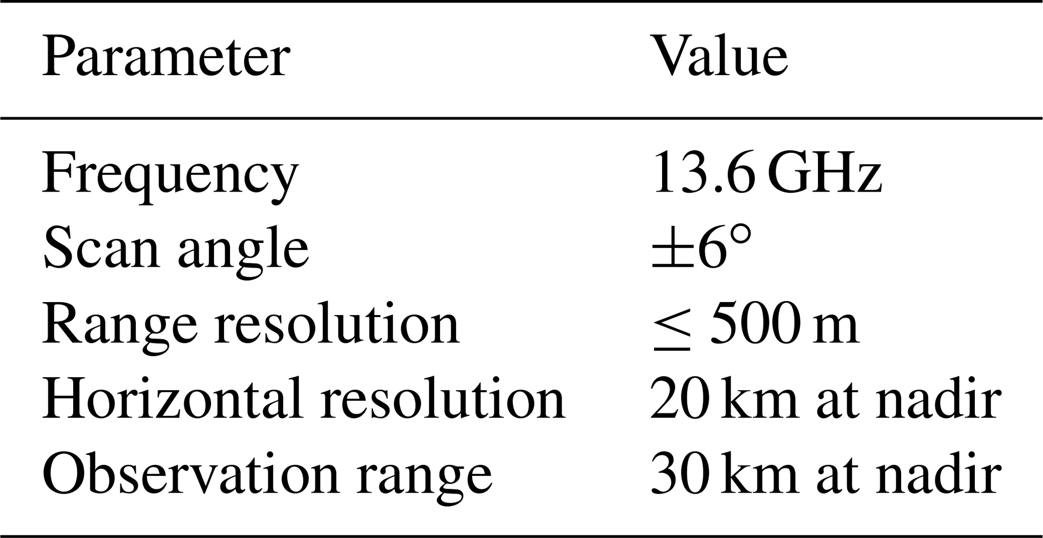
The specifications of GPR are summarized in Table 1. The GPR is anticipated at 13.6 GHz, the same as KuPR on board GPM Core Observatory. We assume a 30 m by 30 m square phased array radar with a half-power beam width (−3 dB) of 0.032∘, with which we can achieve horizontal resolution of 20 km at the nadir point on the Earth's surface. The range resolution is 500 m. Though shorter-range resolution is technically viable, we adopt this value by considering the balance to the horizontal resolution. The number of range bins is 60; the corresponding height of the beam center ranges from the surface to 30 km at nadir. The scan angle is ±6∘, which covers a circular disk with a diameter of 8400 km on the Earth's surface. If the GPR were placed 135∘ E of the Equator, it would cover Sumatra to New Caledonia and Australia to the southern half of Japan.
We assume that the satellite can complete the full disk scan within 1 h. In addition to the normal mode, it is expected to have several modes and can observe a targeting precipitation system intensively as in Himawari-8 (Bessho et al., 2016). In this study, we focus only on snapshots and do not consider the time for GPR to complete the full disk scan.
Table 1Specifications of the precipitation radar aboard geostationary satellite.
2.2 Precipitation reflectivity
This subsection describes how to calculate reflectivity measured by GPR (Z). First, we convert model hydrometeors (cloud water, cloud ice, rain, snow, and graupel) to total backscattering () and extinction coefficients () at every model grid point using an existing software called Joint Simulator for Satellite Sensors (Joint-Simulator; Hashino et al., 2013). The Joint-Simulator is a suite of software that simulates satellite observations based on atmospheric states simulated by cloud-resolving models. The total backscattering and extinction coefficients are obtained respectively by summing single-particle backscattering () and extinction coefficients () for the ith hydrometeor species following its drop size (D) distribution (N(D)) as follows:
where nspec is the number of the hydrometeor species. In this study, up to five hydrometeor species, i.e., cloud water, cloud ice, rain, snow, and graupel, were considered. The Mie approximation is used to calculate and for all the species (Masunaga and Kummerow, 2005). After calculating and at every model grid point, the grid point values are integrated over the scattering volume following the antenna pattern. The radar-received power from precipitation (Pr) of the beam pointing range r0 and scan angle θ0 and ϕ0 is given by
where Pt is the transmitted power, c the speed of light, τ the pulse duration, and f4 the two-way effective beam weighting function. We assumed the uniform antenna pattern, whose sidelobe level is −13.26 dB:
where , Ψ is obtained by solving the equation , and θB is the half-power beam width (−3 dB). is the attenuation factor from the radar to range r in the direction of (θ,ϕ) and is calculated by
The radar reflectivity measured by GPR is calculated as follows:
where λ is the wavelength and K the function of a complex refractivity index of scattering particles. Following Masunaga and Kummerow (2005), |K|2 is assumed to be a constant (0.925) in this study. We do not consider the impact of attenuation (AP=1.0 everywhere) in Sects. 3, 4, and 5 as it can be corrected with proper methods (e.g., Iguchi et al., 2000).
2.3 Surface clutter
Surface clutter echoes contaminate the precipitation signals. In this study, we assumed that the surface is completely covered by the ocean for simplicity. Radar-received power from the sea surface (Ps) was calculated by
where σ0 is the normalized radar cross section (NRCS) of the ocean surface, and S the scattering area. We obtained σ0 using a model proposed by Wentz et al. (1984) based on observations from a microwave scatterometer on board the Seasat satellite. The model expresses σ0 as
where U10 is the 10 m wind speed, and b0 and b1 are fitted parameters. The NRCS for various wind speed is shown in Fig. 2. When raindrops hit the ocean surface, they change the properties of the surface and the scattering signals (Bliven et al., 1997). The impact of impinging rain is negligible at high wind speed (e.g., Braun et al., 1999; Contreras et al., 2003). Since this study focuses on a typhoon case accompanying strong winds, we do not consider the impact of impinging rain. Also, we do not consider the impact of sidelobe clutter in Sects. 3, 4, and 5 as it can be filtered with proper methods (e.g., Kubota et al., 2016).
To understand the characteristics of the radar observation, we first show the results from an idealized case, in which we assume the atmosphere below 2 km is uniformly filled with a certain amount of hydrometeor. We tested five cases: 20, 30, 40, 50, and 60 dBZ. The corresponding precipitation intensity is roughly 1, 2, 5, 20, and 60 mm h−1 if the hydrometeor consists of only rain. The 10 m wind speed was fixed at 10 m s−1 uniformly for all cases. The horizontal resolution of the radar was assumed to be 20 km at the nadir point.
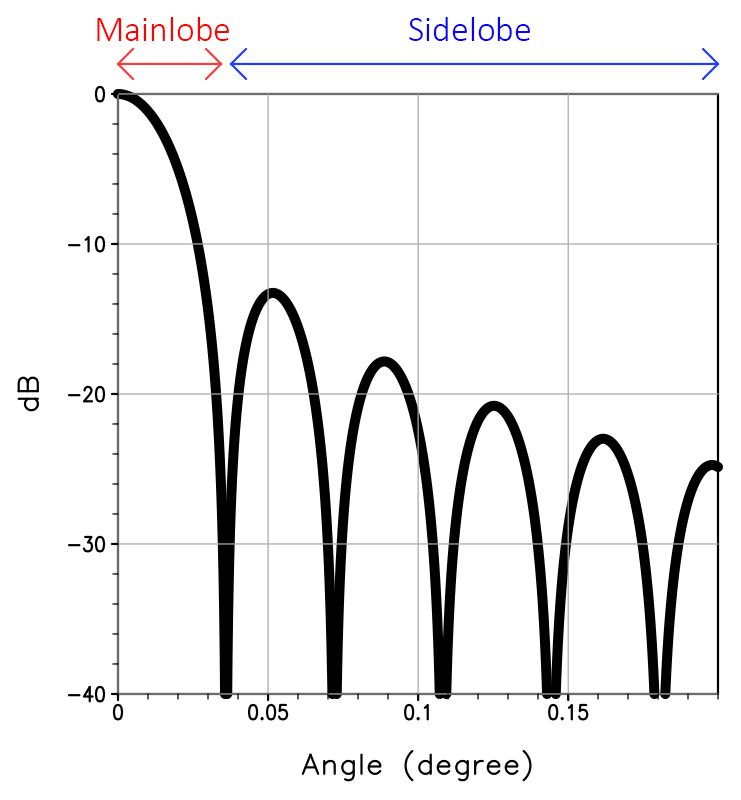
Figure 3a shows Pr for the case of 60 dBZ. Two features are apparent in the figure. The first is that the precipitation signal is beyond the precipitation area and becomes taller along with the distance from the nadir, and the second is that Pr decreases monotonically with height. From here on, the distance was measured along the Earth's surface.
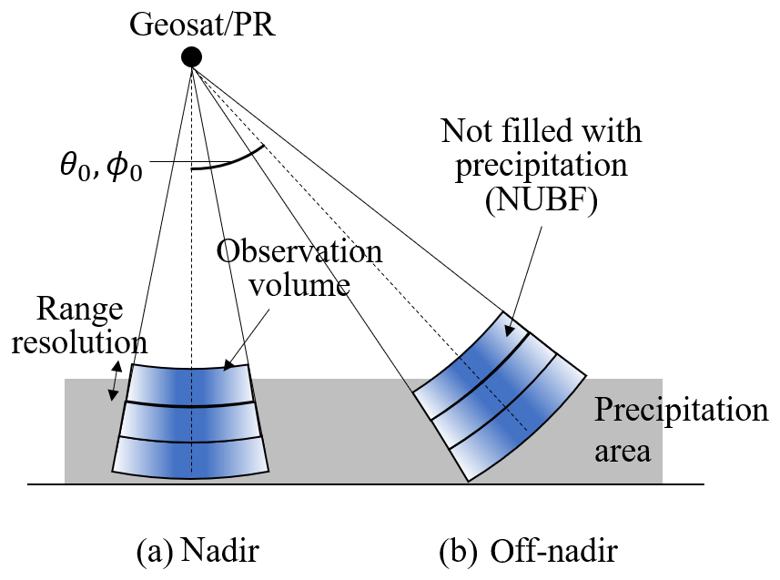
Before discussing the reason for this, first we explain the scattering volume of the GPR. Here, the scattering volume of the beam pointing range r0 and scan angle θ0 and ϕ0 is defined as the area where r, θ, and ϕ satisfy both and ψ less than the first null point (Fig. 1). Note that sidelobe area is not included in the scattering volume in this section. Figure 4 shows a schematic of the scattering volume. At the nadir, the incidence angle is zero, and the scattering volume is nearly parallel to the Earth's surface (Fig. 4a). As the incidence angle increases, the scattering volume becomes tilted against the Earth's surface (Fig. 4b). As a result, the upper edge of the scattering volume reaches as high as 16 km when the beam center of the GPR is at a point 4000 km away from the nadir, even in the lowest range bin (range bin number 1 in Fig. 5b). In the same angle but the highest range bin, the scattering volume ranges from 4 to 38 km in height (range bin number 60 in Fig. 5b). The range of the scattering volume is even larger with sidelobe area.
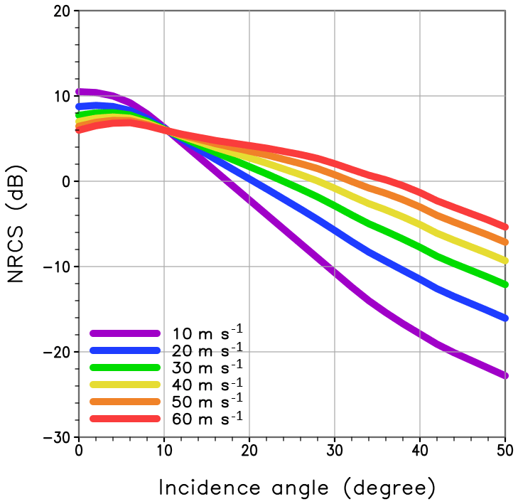
Figure 2Normalized radar cross section (dB) as a function of incidence angle for six cases of 10 m wind speed.
When the beam center is at the level higher than the precipitating area, there is no precipitation around the beam center. On the other hand, the tip of the scattering volume may touch the precipitating area with the tilted scattering volume at off-nadir. In such a case, the scattering volume is not fully filled with precipitation. Such nonuniform beam filling (NUBF) results in the reduction of Pr, with in the upper part of the volume compared with the fully filled case. Although the value is small, GPR still catches the signal of precipitation, and thus Pr has a value even when the beam center is at a point higher than the precipitating area. As the scattering volume becomes more tilted against the Earth's surface along with the distance from the nadir (Fig. 5a), the maximum height at which the beam gets a signal from precipitation becomes higher along with the distance from the nadir. Hence, we have the signal beyond the precipitation area, and the area becomes taller along with the distance from the nadir.
The Pr magnitude dependence on the height is also explained by the NUBF. Due to the experimental setting where precipitation exists only in the atmosphere below 2 km, the beam with the scattering volume touching the level higher than 2 km is not fully filled with precipitation. The higher the GPR observes, the less the scattering volume is filled with precipitation. Accordingly, Pr decreases with height.
The pattern of Ps is similar to that of Pr, showing dependence on the distance from the nadir (Fig. 3b) because σ0 is a function of the incidence angle (Fig. 2).
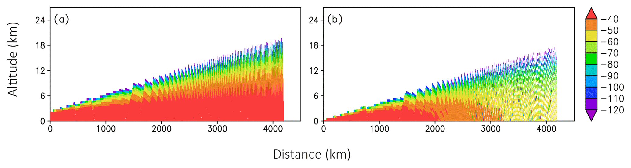
Figure 3Received power from (a) precipitation and (b) sea surface clutter, normalized by Pt (dB).
Figure 6 shows the signal-to-clutter ratio (SCR) defined as Pr∕Ps (dB). The larger the SCR, the less contaminated the signal by the clutter. In the figure, areas where the reflectivity from precipitation exceeds 0 dBZ are shaded. For all the cases, the SCR is the largest at nadir and high altitudes. The minimum SCR is found at the surface level around 500 km away from the nadir, reflecting the peak of the echo from the surface clutter. As expected, the SCR becomes large when precipitation is strong since the received power from the precipitation becomes larger, while Ps is the same for all the cases. The GPR can perceive precipitation only at the nadir point and high altitudes in the case of 20 dBZ (Fig. 6a), but the SCR is larger than zero over the whole precipitating area in the case of 60 dBZ (Fig. 6e) except for the surface level 0 to 1000 km away from the nadir. The comparison of the two cases also suggests that the surface clutter contaminates the precipitation signal from high altitudes for weak precipitation. On the other hand, if the precipitation is strong enough, the clutter interference is limited, and we should get the signal even at the surface level.
The simulated results are consistent with Takahashi (2017) and Li et al. (2017), suggesting that both results are plausible.
Section 3 presented the characteristics of reflectivity of GPR. However, what we can observe will depend on the size and structure of the target precipitation system. To investigate the capability of GPR in detail, we ran an atmospheric model and applied the radar simulator to produce synthetic observations of reflectivity. As an example, we chose Typhoon Soudelor in 2015, which was the strongest typhoon in that year. Soudelor, generated on 1 August 2015 around the Marshall Islands, rapidly intensified to a super typhoon, equivalent to a Category 5 hurricane, within 24 h from generation and dissipated on 11 August 2015. In this study, we focused on the mature stage of Soudelor at 00:00 UTC on 5 August 2015.
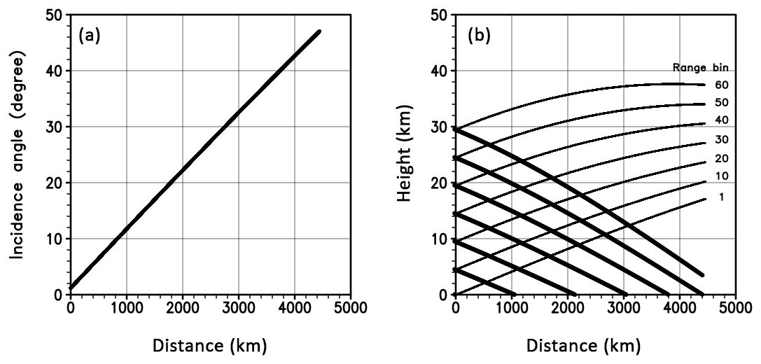
Figure 5Incidence angle (a) and height of the radar scattering volume (b) as a function of the distance from the nadir. Thick and thin lines in (b) show the lower and upper bound, respectively.
In this section, we focus on the sensitivity to two radar parameters: beam width and beam sampling span. Three cases were examined: the first adopts the beam width and sampling span of 20 km, the experiment named “bw20bs20”. The second uses 20 km resolution of beam width, but the beam span is chosen to be 5 km (bw20bs05), representing an over-sampling case. The third uses the 5 km beam width and span (bw05bs05). Although it is unrealistic to assume a radar with the 5 km beam width at this moment, exploring what kind of observations we can get with the 5 km beam width would be beneficial for the antenna design in the future. The radar settings are summarized in Table 2.
Table 2Radar settings. The figures show the resolution at the nadir point.

4.1 SCALE-RM simulation
We used a regional cloud-resolving model, SCALE-RM version 5.0.0 (Nishizawa et al., 2015; Sato et al., 2015) to simulate Soudelor. SCALE-RM is based on the SCALE library for weather and climate simulations. The source code and documents of the SCALE library including SCALE-RM are publicly available at http://r-ccs-climate.riken.jp/scale/ (last access: 10 July 2019). The moist physical process is parameterized by a six-class single-moment bulk microphysics scheme (Tomita et al., 2008), and the five species of hydrometeors (rain, cloud water, cloud ice, snow, and graupel) were used to calculate the radar reflectivity. We use the level 2.5 closure of the Mellor–Yamada–Nakanishi–Niino turbulence scheme to represent subgrid-scale turbulence (Nakanishi and Niino, 2004). For shortwave and longwave radiation processes, the Model Simulation Radiation Transfer code (MSTRN) X (Sekiguchi and Nakajima, 2008) is used. See http://r-ccs-climate.riken.jp/scale/ (last access: 10 July 2019) for more details.
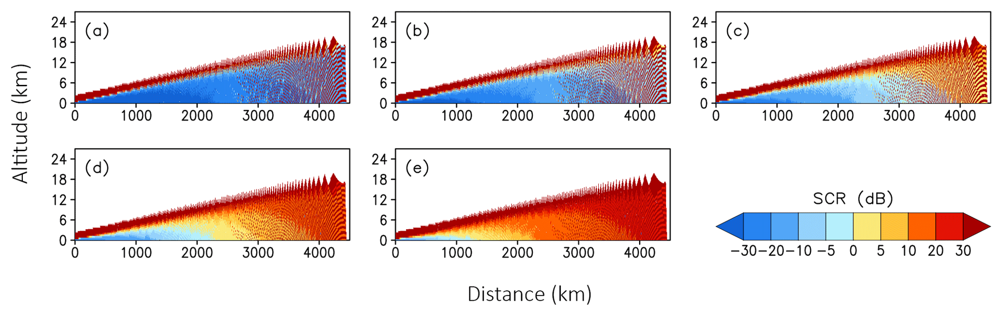
Figure 6Signal-to-clutter ratio (SCR) in measuring five precipitation intensities at (a) 20, (b) 30, (c) 40, (d) 50, and (e) 60 dBZ as a function of the distance from the nadir (km). It is assumed that altitudes lower than 2 km are filled with homogeneous precipitation.
We performed an offline nesting simulation. The horizontal grid spacings and the number of vertical levels for the outer (inner) domain were 15 km (3 km) and 36 levels (56 levels), respectively. Hereafter, the simulation for the outer (inner) domain is referred to as D1 (D2) (Fig. 7a). The initial and lateral boundary conditions for D1 were taken from the National Centers for Environmental Prediction (NCEP) Global Forecasting System (GFS) operational analyses at 0.5∘ resolution every 6 h. The initial and lateral boundary conditions for D2 were taken from D1. The simulation covers the period from 00:00 UTC on 28 July 2015 (00:00 UTC 28 July 2015) to 00:00 UTC on 9 August 2015 (00:00 UTC 7 August 2015) for D1 (D2).

Figure 7(a) Model domains for D1 (blue) and D2 (red) and typhoon tracks and (b) time series of minimum sea level pressure (MSLP). Black, blue, and red colors show the JMA best track data, D1 simulation, and D2 simulation, respectively. Closed and open circles in (a) denote the typhoon positions at 00:00 UTC and 12:00 UTC, respectively.
Figure 7 shows the Soudelor's track and minimum sea level pressure (MSLP) at the typhoon center from the best track of the Japan Meteorological Agency (JMA) and the D1 and D2 simulations. The JMA best track shows a rapid decrease of MSLP during the three days from 1 August. D1 captures the rapid intensification, while D2 shows a slightly slower intensification than the best track. As for the track, both D1 and D2 closely follow the best track albeit slightly shifted northward. We used D2 as a reference to simulate radar observations.
4.2 Results
Figures 8 and 9 show radar reflectivity near the surface level and its vertical cross section in a mature stage of the simulated Soudelor (00:00 UTC, 5 August 2015). The results are shown in the longitude–latitude coordinates for Fig. 8a and in the scan-angle coordinates of the GPR for Fig. 8b–d, covering the same domain as Fig. 8a. As in the homogeneous case, areas where the reflectivity from precipitation exceeds 0 dBZ are shaded in gray.
Figures 8a and 9a show the reflectivity of the full-resolution nature run for reference. The figures show the typical structure of a tropical cyclone characterized by no rainfall within the eye, heavy rainfall in the eye wall, and the spiral outer-rainband structure.
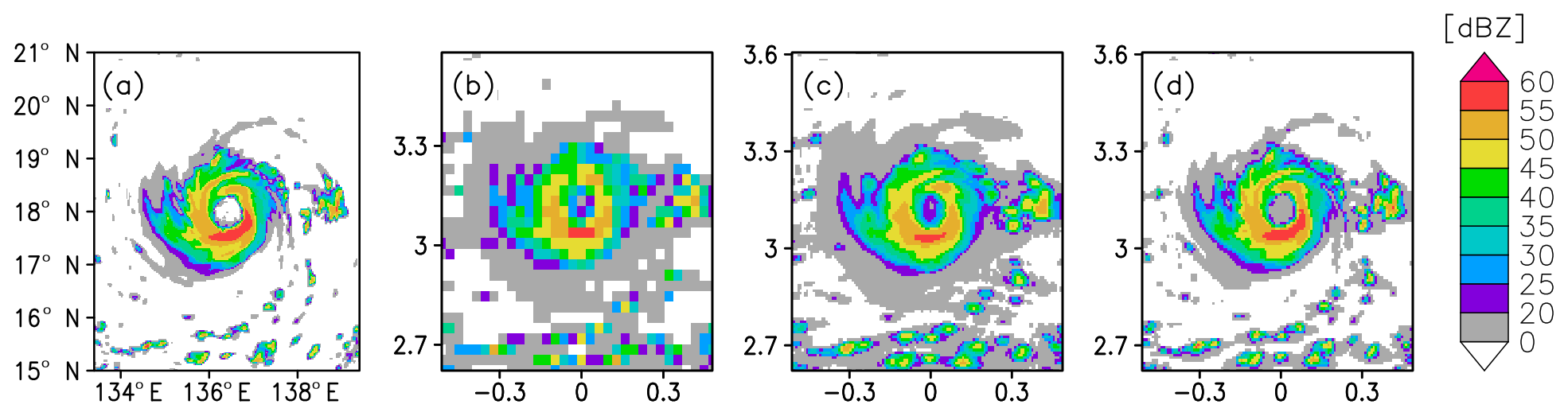
Figure 8Radar reflectivity (dBZ) near the surface in the typhoon mature stage (00:00 UTC, 5 August 2015) for (a) the truth, (b) bw20bs20, (c) bw20bs05, and (d) bw05bs05. 10 m wind speed is overlaid in (a). The areas where reflectivity from precipitation < 0 dBZ are left blank.
The bw20bs20 captures the spatial distribution well but without fine structures. The difference is noticeable in the outer rainband (gray-colored area) in which the shape of the bands is different from the reference. With the tilted and relatively large scattering volume, the radar catches the signal of precipitation that is in the level higher than the level shown in the figure. The bw20bs20 also misses the local maxima of precipitation. For instance, the strongest precipitation south of the eye (red area in Fig. 8a) was not well captured by bw20bs20. This is because the echo from sharp and strong precipitation was averaged out due to NUBF within the relatively large scattering volume. For the vertical cross section, the observation roughly captures the structure albeit in a jaggy and discretized manner because of the tilted and relatively large scattering volume (Fig. 9b). The tilted scattering volume also results in the precipitation echo taller than the reference as discussed in Sect. 3.
On the other hand, the satellite observes precipitation accurately for both spatial and vertical cross sections in bw05bs05 (Figs. 8d and 9d).
In the case of bw20bs05 (i.e., oversampling case), the radar inherited the shortcomings in bw20bs20 due to the wide beam width: the larger precipitated area in the outer rainband (Fig. 8c) and taller precipitation pattern (Fig. 9c) compared with the reference. On the other hand, the results were arguably improved thanks to the fine sampling span compared with bw20bs20. For instance, the strong precipitation south of the eye was well captured compared with bw20bs20 (Fig. 9c). Furthermore, individual convective cells south of the typhoon were observed as individual cells, although they were blurred due to NUBF within the large scattering volume. This is because the finer sampling span increased the probability for the beam center to hit the area of heavy rainfall.

Figure 9Precipitation reflectivity (dBZ) along the 136.4∘ E longitude line passing through the typhoon center in the mature stage (00:00 UTC, 5 August 2015) for (a) the truth, (b) bw20bs20, (c) bw20bs05, and (d) bw05bs05. The areas where reflectivity from precipitation < 0 dBZ are left blank, and the area in which the SCR < 0 is hatched in (b)–(d).
To compare the skills quantitatively, we computed the threat scores with a threshold of 20, 30, 40, and 50 dBZ for all the experiments. Figure 10 shows that bw05bs05 is the best and also shows the benefit of oversampling; namely, the score of bw20bs05 increased by more than 20 % on average for all the thresholds compared with that of bw20bs20.
Figures 9 and 10 also show the impact of the surface clutter. The hatched area in Fig. 9 shows the area where the SCR is less than or equal to zero. Assuming that the SCR of zero is the minimum threshold to indicate whether the clutter interference will be serious (Li et al., 2017), the hatched area is considered unobservable. The unobservable area was confined up to 3 km in bw05bs05, while it reached as high as 7 km in bw20bs20 and bw20bs05. Thus, to reduce the impact of the surface clutter, the beam width needs to be narrow enough.
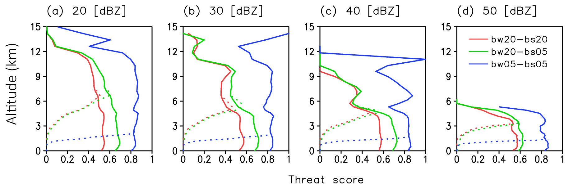
Figure 10Threat score with a threshold of (a) 20, (b) 30, (c) 40, and (d) 50 (dBZ) for bw20bs20 (red), bw20bs05 (green), and bw05bs05 (blue). The dotted and solid lines show the threat score with and without considering the impact of surface clutter, respectively.
Other than at the nadir point, the radar observes precipitation obliquely, and consequently the precipitation echo is easily contaminated by the surface clutter. As mentioned in Sect. 3, how severely surface clutter contaminates the precipitation echo depends on the incidence angle of the beam, which corresponds to the distance from the nadir. Therefore, the location of the target precipitation system should have an impact on the quality of the observations. This section investigates the sensitivity to the location of the typhoon.
We used the simulated Typhoon Soudelor as the reference as in Sect. 4. We picked out the mature stage of the typhoon whose center is in 18∘ N, 136∘ E as an example and moved it north and south to represent typhoons whose center is in 10, 20, and 30∘ N. We assumed the longitudinal position of the typhoon centers were the same as the sub-satellite point for all the cases to compare the difference originating from the latitudinal position of the typhoon center. The radar used in this section was the same as the one in the bw20bs05.
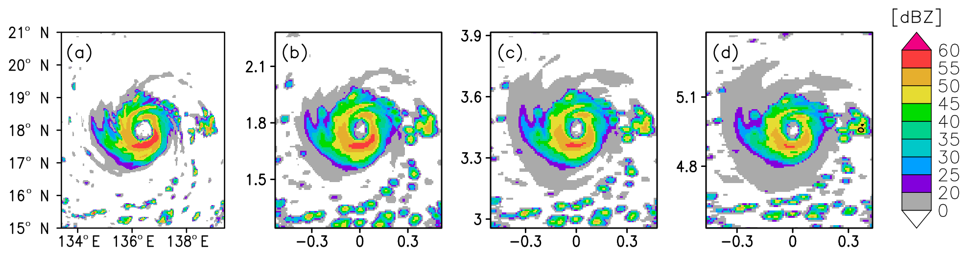
Figure 11Precipitation reflectivity (dBZ) measured with bw20bs05 for the typhoons whose center is in (b) 10∘ N, (c) 20∘ N, and (d) 30∘ N. Contours in (b)–(d) correspond to the area in which the SCR > 0. Panel (a) shows the truth. The areas where reflectivity from precipitation < 0 dBZ are left blank.
Figure 11 shows the precipitation echo at the near-surface level for the three cases together with the reference. Among them, the precipitation pattern in 10∘ N was the most similar to the reference, and the threat score was the highest (Fig. 13). As the typhoon position is away from the sub-satellite point, the precipitation is observed to be weaker with the outer-rainband area more expanded, and the threat score becomes lower (Fig. 13). As discussed in the previous sections, this is due to the widely tilted scattering volume with which the beam captures the signal of precipitation in high altitude whose intensity is weaker than that in the level shown (see Fig. 12). The tilted scattering volume also resulted in vertically extended precipitation echo (Fig. 12). The further away from the nadir, the more vertically extended the precipitation echo. This is also true for the clutter height (SCR≤0): the further away from the nadir, the higher the clutter height. However, this is only the case for areas with weak precipitation. In areas with heavy precipitation at higher latitudes, the impact of the surface clutter is limited to the near-surface level. For instance, the strongest precipitation in the south of the eye is not affected by the surface clutter at all in the case of 30∘ N (Fig. 12d), while it is masked by the clutter in the cases of 10 and 20∘ N (Fig. 12b and c). These results are also evident in the threat score (dashed line in Fig. 13). The surface clutter is determined by the cross section σ0 integrated over the scattering area A, and both σ0 and A decrease along with the incidence angle in this area. Therefore, the echo from the sea surface clutter becomes smaller, and the SCR becomes larger along with the latitude.

Figure 12Precipitation reflectivity (dBZ) along the 136.4∘ E longitude line passing through the typhoon center measured with bw20bs05 for the typhoons whose center is in (b) 10∘ N, (c) 20∘ N, and (d) 30∘ N. Panel (a) shows the truth. The areas where reflectivity from precipitation < 0 dBZ are left blank, and the area in which SCR < 0 is hatched in (b)–(d).
We obtained similar results, as shown in Sect. 3 for the typhoon case. When the observation target is in low latitudes (i.e., close to the nadir), the clutter height is low, and the radar can observe weak precipitation free from clutter at high altitudes. It should be difficult to observe precipitation at the near-surface level, even if the precipitation is strong. In the case the radar observes precipitation in midlatitudes (i.e., away from the nadir), the radar cannot observe weak precipitation at most altitudes, while it is easier to observe strong precipitation at any altitude.
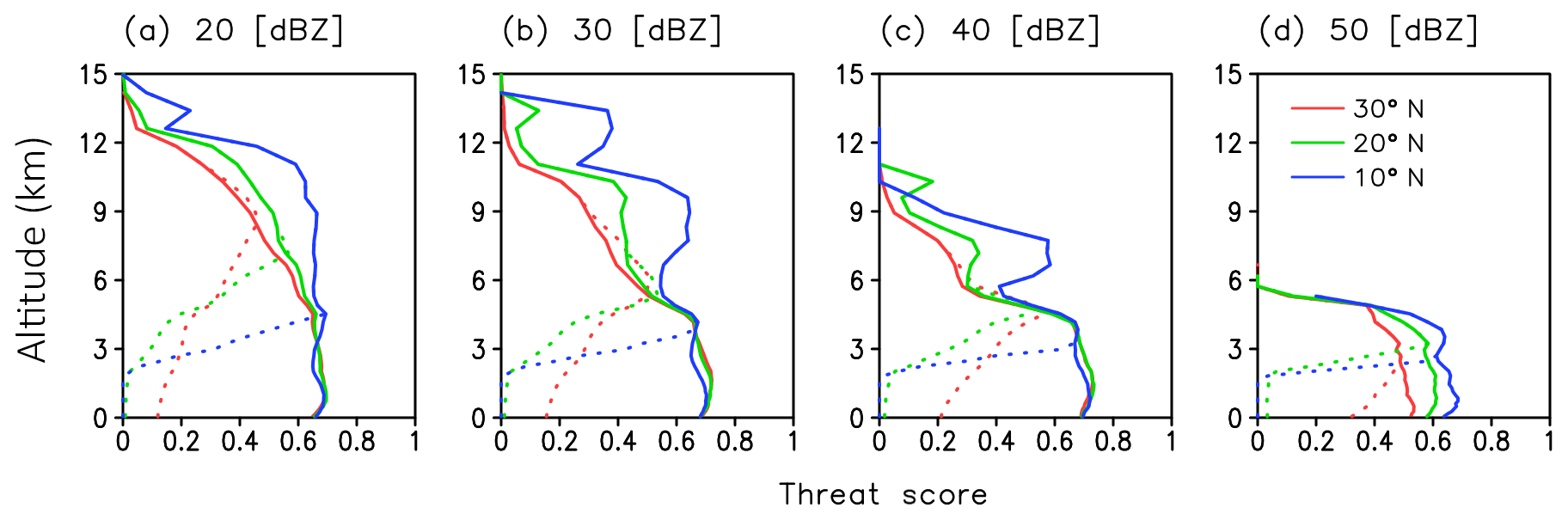
Figure 13Threat score with a threshold of (a) 20, (b) 30, (c) 40, and (d) 50 (dBZ) for the typhoons whose centers are in 30∘ N (red), 20∘ N (green), and 10∘ N (blue). The dotted and solid lines show the threat score with and without considering the impact of surface clutter, respectively.
In the previous sections, we did not consider the impact of attenuation and sidelobe clutter, assuming that they can be corrected (e.g., Iguchi et al., 2000) or filtered (e.g., Kubota et al., 2016). In this section, we investigate the impact of attenuation and sidelobe clutter. To consider attenuation, the attenuation coefficient is included in the calculation of Pr, Ps, and Z (Eqs. 3, 6, and 7). The attenuation coefficients are calculated with Eq. (5), and the extinction coefficients are calculated by Joint-Simulator (Hashino et al., 2013). To investigate the impact of sidelobe clutter, the observation volume is expanded to include the sidelobe area up to the fifth null point (Fig. 1).
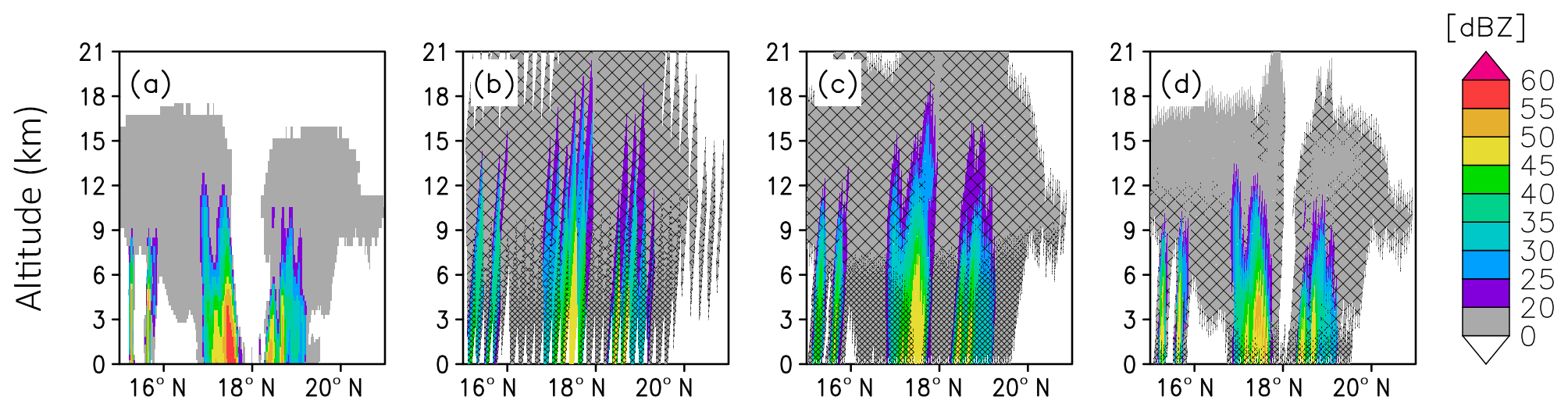
Figure 14Precipitation reflectivity (dBZ) along the 136.4∘ E longitude line passing through the typhoon center in the mature stage (00:00 UTC, 5 August 2015) for (a) the truth, (b) bw20bs20, (c) bw20bs05, and (d) bw05bs05. The areas where reflectivity from precipitation < 0 dBZ are left blank, and the area affected (SCR < 0) by mainlobe (sidelobe) clutter is densely (sparsely) hatched in (b)–(d).
Figure 14 shows the cross section of the typhoon with various radar parameters: bw20bs20, bw20bs05, and bw05bs05. Due to the attenuation, reflectivity from heavy rain is weakened for all the cases (e.g., the reflectivity at south of the eye). This feature is also evident in the threat score for the case with bw20bw05 (Fig. 15). Figure 15 compares three cases: The first case (“main”) does not consider the impact of attenuation, and its observation volume does not include the sidelobe area, i.e., the same as the bw20bs05 in Fig. 10. The second case (“main + side”) does not consider the impact of attenuation, but its observation volume includes the sidelobe area; i.e., it considers the impact of sidelobe clutter. The third case (“main + atten.”) considers the impact of attenuation, but its observation volume does not include the sidelobe area. Figure 15 shows that the threat score of main + atten. is almost identical to that of main, and the impact of attenuation is negligible for the thresholds of 20, 30, and 40 dBZ. On the other hand, the threat score of main + atten. with the threshold of 50 dBZ is zero at all heights. Therefore, the attenuation makes it difficult to obtain rain echoes from strong precipitation.

Figure 15Threat scores with thresholds of (a) 20, (b) 30, (c) 40, and (d) 50 (dBZ) for bw20bs05. The red line overlaps the blue line for (a), (b), and (c) and the green line for (d). The dotted and solid lines show the threat score with and without considering the impact of surface clutter, respectively.
On the other hand, the sidelobe clutter contaminates the weak to moderate rain echoes. For example, the top of convection at around 17∘ N is masked by the sidelobe clutter for the cases with low-resolution beam (Fig. 14a and b). Figure 15 also shows that threat scores of main + side are smaller than that of main for the thresholds of 20, 30, and 40 dBZ, while the impact is negligible for the threshold of 50 dBZ. Therefore, the sidelobe clutter contaminates weak to moderate rain.
We examined the feasibility of radar observation for precipitation from a geostationary satellite. The results demonstrated that it would be possible to obtain three-dimensional precipitation data. However, the quality of the observation was found to depend on the beam width, the beam sampling span, and the position of targeting precipitation systems. With the wide beam width and coarse beam span, the radar cannot observe weak precipitation at low altitudes. The limitations can be somewhat mitigated by oversampling (i.e., a wide beam width but a fine sampling span). With the narrow beam width and fine beam sampling span, the surface clutter interference was confined to the surface level. For the position of the target precipitation system, the larger (smaller) the off-nadir angle, the easier (more difficult) it is to obtain the precipitation signal if the precipitation is strong (weak).
This study also investigated the impact of attenuation and sidelobe clutter. The attenuation hinders obtainment of rain echoes from strong precipitation, while the sidelobe clutter contaminates signals from weak precipitation. An attenuation correction method like the surface-reference method (e.g., Iguchi et al., 2000; Meneghini et al., 2000) and a clutter filter (e.g., Kubota et al., 2016) must be devised to mitigate the detrimental impacts. One possible idea for the filter may be to distinguish an echo from precipitation and surface by using the Doppler shift, but this remains to be a subject of future research.
If the wide beam width of 0.032∘ is used, the raw product may be prohibitively coarse for a specific purpose. One possible way to effectively downscale such observations is to assimilate the data for NWP. By doing this, the information can be treated properly, and we can get precipitation information in the prediction model coordinate. However, it is not trivial whether assimilation of such data is useful for NWP. In the future, an observing system simulation experiment (OSSE) will be conducted using precipitation measurements simulated with the simulator developed in this study to evaluate the potential impacts of the GPR on NWP. Given that wind field observation may be possible from a geostationary satellite as shown in Lewis et al. (2011), the combined use of both observations would be an attractive option.
SCALE-RM is available at http://r-ccs-climate.riken.jp/scale/ (last access: 11 July 2019). Joint-Simulator is available at https://www.eorc.jaxa.jp/theme/Joint-Simulator/userform/js_userform.html (last access: 11 July 2019).
TM is the PI and directed the research. AO, MY, TK, RO, TI, and TM designed the study. AO, TH, KS, and TI carried out the analysis. AO prepared the manuscript with contributions from all the co-authors.
The authors declare that they have no conflict of interest.
This study was partly supported by the Japan Aerospace Exploration Agency (JAXA) and the FLAGSHIP2020 Project of the Ministry of Education, Culture, Sports, Science and Technology of Japan. The experiments were performed using the K computer at the RIKEN R-CCS (ra000015, hp160229, hp170246, hp180194).
This research has been supported by the Japan Aerospace Exploration Agency (grant nos. JX-PSPC-435434, JX-PSPC-456242, and JX-PSPC-501630) and the Ministry of Education, Culture, Sports, Science and Technology (FLAGSHIP2020 Project).
This paper was edited by Saverio Mori and reviewed by two anonymous referees.
Bell, T. L., Abdullah, A., Martin, R. L., and North, G. R.: Sampling errors for satellite-derived tropical rainfall: Monte Carlo study using a space-time stochastic model, J. Geophys. Res., 95, 2195–2205, 1990.
Bessho, K., Date, K., Hayashi, M., Ikeda, A., Imai, T., Inoue, H., Kumagai, Y., Miyakawa, T., Murata, H., Ohno, T., Okuyama, A., Oyama, R., Sasaki, Y., Shimazu, Y., Shimoji, K., Sumida, Y., Suzuki, M., Taniguchi, H., Tsuchiyama, H., Uesawa, D., Yokota, H., and Yoshida, R.: An introduction to Himawari-8/9: Japan's new-generation geostationary meteorological satellites, J. Meteorol. Soc. Jpn., 94, 151–183, 2016.
Bliven, L. F., Sobieski, P. W., and Craeye, C.: Rain generated ring-waves: Measurements and modelling for remote sensing, Int. J. Remote. Sens., 18, 221–228, 1997.
Braun, N., Gade, M., and Lange, P. A.: Radar backscattering measurements of artificial rain impinging on a water surface at different wind speeds, paper presented at 1999 International Geoscience and Remote Sensing Symposium (IGARSS), Inst. of Elect. and Elect. Eng., New York, 1999.
Contreras, R. F., Plant, W. J., Keller, W. C., Hayes, K., and Nystuen, J., Effects of rain on Ku-band backscatter from the ocean, J. Geophys. Res., 108, 3165, https://doi.org/10.1029/2001JC001255, 2003.
Hamada, A., Takayabu, Y. N., Liu, C., and Zipser, E. J.: Weak linkage between the heaviest rainfall and tallest storms, Nat. Commun., 6, 6213, https://doi.org/10.1038/ncomms7213, 2015.
Hashino, T., Satoh, M., Hagihara, Y., Kubota, T., Matsui, T., Nasuno, T., and Okamoto, H.: Evaluating cloud microphysics from NICAM against CloudSat and CALIPSO, J. Geophys. Res.-Atmos., 118, 7273–7292, 2013.
Hou, A. Y., Kakar, R. K., Neeck, S., Azarbarzin, A. A., Kummerow, C. D., Kojima, M., Oki, R., Nakamura, K., and Iguchi, T.: The global precipitation measurement mission, B. Am. Meteor. Soc., 95, 701–722, 2014.
Houze, R. A., Rasmussen, K. L., Zuluaga, M. D., and Brodzik, S. R.: The variable nature of convection in the tropics and subtropics: A legacy of 16 years of the Tropical Rainfall Measuring Mission satellite, Rev. Geophys., 53, 994–1021, 2015.
Iguchi, T., Kozu, T., Meneghini, R., Awaka, J., and Okamoto, K.: Rain-profiling algorithm for the TRMM precipitation radar, J. Appl. Meteorol., 39, 2038–2052, 2000.
Im, E., Smith, E. A., Chandrasekar, V. C., Chen, S., Holland, G., Kakar, R., Tanelli, S., Marks, F., and Tripoli, G.: Workshop report on NEXRAD-In-Space – A geostationary satellite doppler weather radar for hurricane studies, 33rd Conf. on Radar Meteorology, Cairns, QLD, Australia, Amer. Meteor. Soc., available at: http://ams.confex.com/ams/pdfpapers/123726.pdf (last access: 11 July 2019), 4B.5, 2007.
Joudoi, D., Kuratomi, T., and Watanabe, K.: The construction method of a 30-m-class large planar antenna for Space Solar Power Systems, 69th International Astronautical Congress, Bremen, Germany, 1–5, October, 2018.
Kelley, O. A., Stout, J., and Halverson, J. B.: Tall precipitation cells in tropical cyclone eyewalls are associated with tropical cyclone intensification, Geophys. Res. Lett., 31, L24112, https://doi.org/10.1029/2004GL021616, 2004.
Kidd, C., Becker, A., Huffman, G. J., Muller, C. L., Joe, P., Skofronick-Jackson, G., and Kirschbaum, D. B.: So, how much of the earth's surface is covered by rain gauges?, B. Am. Meteorol, Soc., 69–78, https://doi.org/10.1175/BAMS-D-14-00283.1, 2016.
Kozu, T., Kawanishi, T., Kuroiwa, H., Kojima, M., Oikawa, K., Kumagai, H., Okamoto, K., Okumura, M., Nakatshka, H., and Nishikawa, K.: Development of precipitation radar onboard the Tropical Rainfall Measuring Mission (TRMM) satellite, IEEE T. Geosci. Remote, 39, 102–116, 2001.
Kubota, T., Iguchi, T., Kojima, M., Liao, L., Masaki, T., Hanado, H., Meneghini, R., and Oki, R.: A statistical method for reducing sidelobe clutter for the Ku-band precipitation radar on board the GPM Core Observatory, J. Atmos. Ocean. Tech., 33, 1413–1428, 2016.
Kummerow, C., Barnes, W., Kozu, T., Shiue, J., and Simpson, J.: The Tropical Rainfall Measuring Mission (TRMM) sensor package, J. Atmos. Ocean. Tech., 15, 808–816, 1998.
Lewis, W. E., Im, E., Tanelli, S., Haddad, Z., Tripoli, G. J., and Smith, E. A.: Geostationary doppler radar and tropical cyclone surveillance, J. Atmos. Ocean. Tech., 28, 1185–1191, 2011.
Li, X., He, J., Wang, C., Tang, S., and Hou, X.: Evaluation of surface clutter for future geostationary spaceborne weather radar, Atmosphere, 8, 14, https://doi.org/10.3390/atmos8010014, 2017.
Masunaga, H. and Kummerow, C.: Combined radar and radiometer analysis of precipitation profiles for a parametric retrieval algorithm, J. Atmos. Ocean. Tech., 22, 909–929, 2005.
Meguro, A., Shintate, K., Usui, M., and Tsujihata, A.: In-orbit deployment characteristics of large deployable antenna reflector onboard Engineering Test Satellite VIII, Acta Astronaut., 65, 1306–1316, 2009.
Meneghini, R., Iguchi, T., Kozu, T., Liao, L., Okamoto. K., Jones, J. A., and Kwiatkowski, J.: Use of the surface reference technique for path attenuation estimates from the TRMM radar, J. Appl. Meteorol., 39, 2053–2070, 2000.
Nakanishi, M. and Niino, H.: An improved Mellor–Yamada level-3 model with condensation physics: Its design and verification, Bound.-Lay. Meteorol., 112, 1–31, 2004.
Nishizawa, S., Yashiro, H., Sato, Y., Miyamoto, Y., and Tomita, H.: Influence of grid aspect ratio on planetary boundary layer turbulence in large-eddy simulations, Geosci. Model Dev., 8, 3393–3419, https://doi.org/10.5194/gmd-8-3393-2015, 2015.
Sato, Y., Nishizawa, S., Yashiro, H., Miyamoto, Y., Kajikawa, Y., and Tomita, H.: Impacts of cloud microphysics on trade wind cumulus: which cloud microphysics processes contribute to the diversity in a large eddy simulation?, Prog. Earth Planet. Sci., 2, 23, 2015.
Sekiguchi, M. and Nakajima, T.: A k-distribution-based radiation code and its computational optimization for an atmospheric general circulation model, J. Quant. Spectrosc. Ra., 109, 2779–2793, 2008.
Skofronick-Jackson, G., Petersen, W. A., Berg, W., Kidd, C., Stocker, E. F., Kirschbaum, D. B., Kakar, R., Braun, S. A., Huffman, G. J., Iguchi, T., Kirstetter, P. E., Kummerow, C., Meneghini, R., Oki, R., Olson, W. S., Takayabu, Y., Furukawa, K., and Wilheit, T.: The global precipitation measurement (GPM) mission for science and society, B. Am. Meteorol. Soc., 98, 1679–1695, 2017.
Takahashi, N.: Surface echo characteristics derived from the wide swath experiment of the precipitation radar onboard TRMM satellite during its end-of-mission operation, IEEE T. Geosci. Remote., 55, 1988–1993, 2017.
Takayabu, Y. N.: Rain-yield per flash calculated from TRMM PR and LIS data and its relationship to the contribution of tall convective rain, Geophys. Res. Lett., 33, L18705, https://doi.org/10.1029/2006GL027531, 2006.
Tomita, H.: New microphysical schemes with five and six categories by diagnostic generation of cloud ice, J. Meteorol. Soc. Jpn., 86A, 121–142, 2008.
Wentz, F. J., Peteherych, S., and Thomas, L. A.: A model function for ocean radar cross sections at 14.6 GHz, J. Geophys. Res., 89, 3689–3704, 1984.