the Creative Commons Attribution 4.0 License.
the Creative Commons Attribution 4.0 License.
 | 14 Aug 2019
Footprint-scale cloud type mixtures and their impacts on Atmospheric Infrared Sounder cloud property retrievals
Alexandre Guillaume
Brian H. Kahn
Eric J. Fetzer
Gerald J. Manipon
Brian D. Wilson
Hook Hua
A method is described to classify cloud mixtures of cloud top types, termed cloud scenes, using cloud type classification derived from the CloudSat radar (2B-CLDCLASS). The scale dependence of the cloud scenes is quantified. For spatial scales at 45 km (15 km), only 18 (10) out of 256 possible cloud scenes account for 90 % of all observations and contain one, two, or three cloud types. The number of possible cloud scenes is shown to depend on spatial scale with a maximum number of 210 out of 256 possible scenes at a scale of 105 km and fewer cloud scenes at smaller and larger scales. The cloud scenes are used to assess the characteristics of spatially collocated Atmospheric Infrared Sounder (AIRS) thermodynamic-phase and ice cloud property retrievals within scenes of varying cloud type complexity. The likelihood of ice and liquid-phase detection strongly depends on the CloudSat-identified cloud scene type collocated with the AIRS footprint. Cloud scenes primarily consisting of cirrus, nimbostratus, altostratus, and deep convection are dominated by ice-phase detection, while stratocumulus, cumulus, and altocumulus are dominated by liquid- and undetermined-phase detection. Ice cloud particle size and optical thickness are largest for cloud scenes containing deep convection and cumulus and are smallest for cirrus. Cloud scenes with multiple cloud types have small reductions in information content and slightly higher residuals of observed and modeled radiance compared to cloud scenes with single cloud types. These results will help advance the development of temperature, specific humidity, and cloud property retrievals from hyperspectral infrared sounders that include cloud microphysics in forward radiative transfer models.
- Article
(2650 KB) - Full-text XML
- BibTeX
- EndNote


© 2019 California Institute of Technology. Government sponsorship acknowledged.
There is increasing evidence of secular cloud trends at regional and global scales in both satellite observations (e.g., Norris et al., 2016) and climate general circulation model (GCM) simulations (e.g., Zelinka et al., 2013). The poleward migration of the extratropical storm tracks (Barnes and Polvani, 2013) is coupled to systematic changes in cloud-thermodynamic-phase partitioning in forced CO2 experiments in climate GCMs (e.g., Mitchell et al., 1989; Ceppi et al., 2016). The spread in equilibrium climate sensitivity is also tightly coupled to the temporal evolution of phase partitioning in most climate GCMs (Tan et al., 2016). Obtaining reasonable observational estimates of the small-scale cloud-phase partitioning at model subgrid scales is critical for constraining the highly uncertain Wegener–Bergeron–Findeisen timescale parameter that is crucial for modeling mixed-phase cloud and precipitation processes (Tan and Storelvmo, 2016). A new generation of probability-distribution-function-based parameterizations has shown promise for improving climate model simulations of cloud properties (e.g., Golaz et al., 2002) and would benefit from further exploitation of the information available in pixel-scale satellite observations. A rigorous assessment of the scale dependence of cloud types, and their mixtures, would also enhance climate GCM evaluation and parameterization development research efforts (Bony et al., 2006).
Kahn et al. (2018) showed that Atmospheric Infrared Sounder (AIRS) observations of ice cloud optical thickness (τi) and effective radius (rei) exhibit statistically significant temporal trends that are dependent on latitude and cloud type. Trends in Multi-angle Imaging SpectroRadiometer (MISR) observations of cloud texture have suggested that recent thinning of tropical cirrus has led to increased detection of trade cumulus (Zhao et al., 2016). Using high-spatial-resolution estimates of cloud thermodynamic phase obtained from the Hyperion instrument on Earth Observing 1 (EO-1), Thompson et al. (2018) showed that phase mixtures are highly variable at scales smaller than the AIRS footprint or typical GCM grid boxes. These studies (and many others) suggest that quantification of the scale dependence of cloud type mixtures could help explain satellite observations of cloud trends.
Statistical classification methods are commonly used to define weather states or cloud types (e.g., Rossow et al., 2005; Xu et al., 2005; Sassen and Wang, 2008; Wang et al., 2016). For instance, joint histograms of cloud top pressure and optical thickness from the International Satellite Cloud Climatology Project (ISCCP; Rossow and Schiffer, 1999) are useful for relating cloud types to dynamical, radiation, and precipitation variability, as well as in evaluating climate model simulations (e.g., Klein and Jakob, 1999; Jakob and Tselioudis, 2003; Rossow et al., 2005; Tselioudis et al., 2013). Weather states are typically mixtures of conventional cloud types as shown by Rossow et al. (2005) and Oreopoulos et al. (2014). Partly inspired by this methodology, we introduce the concept of cloud scenes that are defined to be mixtures of CloudSat cloud types (2B-CLDCLASS; Sassen and Wang, 2005) that vary with horizontal scale.
As cloud scenes will be matched to coincident A-Train observations, we begin by defining cloud scenes with cloud types derived from CloudSat and observed within an AIRS/Advanced Microwave Sounding Unit (AMSU) (Chahine et al., 2006) field of regard (FOR) of roughly 45 km resolution. One AMSU FOR within an AMSU swath is spatially and temporally coincident with a “curtain” of 94 GHz CloudSat radar profiles. The likelihood of observing clouds is resolution-dependent and is approximately 80 %–85 % at the AIRS footprint scale of 15 km (Krijger et al., 2007; Kahn et al., 2008). The clouds in AMSU sounding FORs or AIRS footprints are more often broken or transparent and less often uniform or opaque. Yue et al. (2013) showed that about 43 % of the AMSU FORs are mixtures of CloudSat-identified cloud types, implying that roughly half of cloudy soundings contain mixtures of cloud types.
Our purpose in this work is to quantify the scale dependence of cloud type mixtures that are then used to understand the cloud complexity within AIRS cloud-phase and ice cloud property data sets. The AIRS and CloudSat data and the collocation approach are described in Sect. 2. To quantify cloud type distributions and their dependence on horizontal scales, the cloud scenes are first characterized at the AMSU FOR resolution in Sect. 3.1, are extended to larger and smaller scales in Sect. 3.2, and key results of the scale dependence are placed into context in Sect. 3.3. The cloud scenes are used to partition AIRS cloud property retrievals into cloud types, specifically, cloud-thermodynamic-phase histograms in Sect. 4.2, and mean values of ice cloud microphysical parameters are described in Sect. 4.3. A discussion, summary, and suggestions for future investigation are found in Sect. 5.
2.1 CloudSat and AIRS pixel-scale matching
The AIRS/AMSU/CloudSat matchup product described in Manipon et al. (2016) is used by Yue et al. (2013) and in this investigation. The matchup process uses a nearest-neighbor approach to geolocate all CloudSat profiles within either an AMSU FOR at 45 km spatial resolution at nadir view or a single AIRS footprint at 15 km spatial resolution at nadir view (Kahn et al., 2008). Approximately 45 to 50 (15–17) CloudSat profiles coincide with a single AMSU FOR (AIRS footprint), in a swath of width 30 FORs (90 footprints). The cloud scenes are first defined at the AMSU FOR scale and are then extended to other spatial scales. We use a 2-year period of data extending from 1 July 2006 until 30 June 2008 which contains about 8 million AMSU FORs (or 24 million AIRS footprints).
2.2 CloudSat cloud types and their mixtures within the AIRS footprint
The CloudSat 2B-CLDCLASS product is used in this work and the algorithm is described in Sassen and Wang (2005, 2008). As summarized in Sassen and Wang (2008) and previous works, the algorithm uses methods developed from ground-based multiple remote sensors that have been tested against surface observer-based cloud typing reports. The cloud classification occurs in two steps. First, a clustering analysis is performed to group cloud profiles into cloud clusters. Secondly, classification methods are used to classify clouds into different cloud types. The decision trees guiding the classification are complex and are based on 23 variables derived from the clustering analysis of the first stage. Geometric quantities such as cloud base, top, and horizontal extents are present in decision trees (Sassen and Wang, 2005). Plan view and zonal average frequencies of 2B-CLDCLASS cloud types at its native resolution are reported in Sassen and Wang (2008).
There are eight CloudSat-defined classes in the 2B-CLDCLASS files: cumulus (Cu), stratocumulus (Sc), stratus (St), altocumulus (Ac), altostratus (As), nimbostratus (Ns), cirrus (Ci), and deep convective (Dc) clouds, with a ninth classification of clear sky designated no cloud (nc). Since each AMSU FOR contains roughly 50 CloudSat profiles with 125 vertical levels each, there are 950×125 possible distinct cloud type combinations (although in practice there are fewer as many levels reside in the stratosphere) for each AMSU FOR. This number is too high to derive a classification that could be useful, i.e., where each cloud type combination could be populated with a significant number of samples for any climatological study. One particularly appealing way to reduce the dimensionality is to limit consideration of cloud type to cloud top only. This simplification is consistent with the capabilities of infrared sounders as the sampling of temperature and specific humidity is maximized in the atmosphere near and above cloud top, assuming the cloud is opaque and covers the entire sounder pixel area. There are 950 possible cloud combinations defined in this manner, including clear sky profiles. As a point of comparison, there are about 324 000 AIRS soundings per day or about 108 per year. Even when considering the 16 years of AIRS nominal operation, the number of cloud type combinations 950, or about 5×1047, is many orders of magnitude greater than the number of AMSU FORs available, making it impossible to perform a statistically significant sampling of all combinations. This necessitates further assumptions to define a practical yet meaningful set of cloud scenes.
Two additional simplifications are made here: variations in the count of each CloudSat cloud type are not considered, and the observation sequence of successive cloud types is disregarded. These two simplifications are applied to the AMSU field of view (FOV). We define a cloud scene as a list of the cloud types that are present within a given AMSU FOR. For example, the notation (Ci, Ac, Sc, Cu) is used to label a cloud scene that contains cirrus, altocumulus, stratocumulus, and cumulus clouds at cloud top in any frequency and in any sequence along the orbit segment. These simplifications greatly reduce the dimensionality of the classification problem and make cloud scene identification tractable. We will show both partly cloudy and completely cloudy scenes in Section 4, so the clear sky (nc) type is both included and excluded in the analyses. Since each of the eight cloud types is either present or absent, a cloud scene can also be represented by an 8 bit binary string. As a consequence, there are 256 (28) possible cloud scenes that remain after taking into account the aforementioned simplifications. The number of possible cloud scenes is therefore reduced from 950×125 to a much more tractable 256. The limitations of this approach are (i) a consideration of cloud tops only, (ii) the spatial sequence and frequency of individual cloud types are not considered, and (iii) equal weight is given to all cloud types within a cloud scene regardless of counts.
One advantage of using a classification to define cloud mixtures rather than an unsupervised learning technique, such as clustering, is that the size of the set of possible cloud mixtures is well defined and finite (here it is 256). A related and important advantage of classification is that one can use this set of classes (cloud scenes) with any parameter matched to any given scene. Here, the spatial-scale dependence of those cloud scenes is described in Sect. 3.2.
An alternative approach may consider the vertical layering of cloud types or cloud features, some form of weighting based on counts of each cloud type, or possibly the sequence of cloud types, which may result in different radiance measurements observed by the AIRS instrument (the radiance emitted within an AIRS footprint is nonuniform and channel-dependent, as described in Schreier et al., 2010). However, the simplified approach outlined above is broadly consistent with the sensitivity and sampling characteristics of nadir-viewing passive infrared sounders. Therefore, we consider the approach outlined above to be an appropriate compromise that retains the diversity of cloud scenes and makes the necessary data processing tractable by reducing the dimensionality for ease of interpretation.
Lastly, the results of Kahn et al. (2018) suggest larger ice cloud particle sizes occur at convective cloud tops compared to thin cirrus at the same cloud top temperature. Given the key assumption of cloud typing only at cloud top, the 2B-CLDCLASS product is better suited for identifying convective clouds in AIRS apart from stratiform clouds, the latter of which are dominant in 2B-CLDCLASS-LIDAR. If 2B-CLDCLASS-LIDAR was used in place of 2B-CLDCLASS, the statistics would be weighted towards the detection of vast areas of cirrus in thin layers above and in proximity to convective clouds. The Ci classification dominates in 2B-CLDCLASS-LIDAR at cloud top and will blur the signals of underlying cumulus and deep convective cloud types that are capped by thin cirrus.
2.3 AIRS thermodynamic-phase and ice cloud properties
The AIRS version 6 cloud-thermodynamic-phase and ice cloud properties (Kahn et al., 2014) are geolocated to the CloudSat ground track and are binned by cloud scene. The cloud-thermodynamic-phase algorithm includes two liquid tests and four ice tests of brightness temperature (Tb) thresholds and Tb differences (ΔTb) in the midinfrared atmospheric windows. The Tb and ΔTb thresholds are designed to exploit spectral differences in liquid and ice water indices of refraction. The two liquid and four ice tests are each assigned a value of −1 and +1, respectively, and a summed value that ranges from −2 to +4 is reported. Summed values −2 or −1 indicate liquid clouds, 0 is undetermined, and values indicate ice, with the highest values indicating deeper, convective ice clouds (Naud and Kahn, 2015). Ice is detected in 26.5 % of AIRS footprints by Kahn et al. (2014), and pixel-scale comparisons with estimates of ice from the Cloud-Aerosol Lidar and Infrared Pathfinder Satellite Observation (CALIPSO) lidar (Jin and Nasiri, 2014) are in agreement with AIRS more than 90 % of the time. The success rate, however, is smaller for liquid cloud detection with AIRS using CALIPSO as a benchmark because of the small thermal contrast between low-lying liquid clouds and the surface. Despite this limitation in sensitivity, AIRS rarely misidentifies liquid clouds as ice (Jin and Nasiri, 2014). Furthermore, many liquid clouds are classified as undetermined phase. Low-latitude shallow trade cumulus clouds generally fall within this category (Kahn et al., 2017).
Kahn et al. (2014) describe a retrieval algorithm that is based on optimal estimation (OE) theory and derives ice cloud optical thickness (τi) and effective radius (rei) for AIRS footprints containing ice. The AIRS retrieval sample includes nearly all ice clouds with τi > 0.1, while the maximum values of τi asymptote to values around 6–8 (e.g., Kahn et al., 2015). Scalar averaging kernels (AKs), χ2 residuals from observed and simulated radiance fits, and values of relative error are also reported (Kahn et al., 2014). Values of AKs closer to 1.0 suggest higher information content, while larger relative error estimates and values of χ2 indicate increased uncertainty in retrieved parameters. Only the relative magnitude of error estimates should be considered since temperature, specific humidity, surface temperature, surface emissivity, and ice crystal habit and size distribution uncertainties are not included in the error covariance matrices of the AIRS version 6 algorithm (see Kahn et al., 2014). We focus on the differences in error estimates and χ2 among cloud scenes and determine which cloud scenes contain higher or lower certainty in their ice cloud properties relative to other scenes.
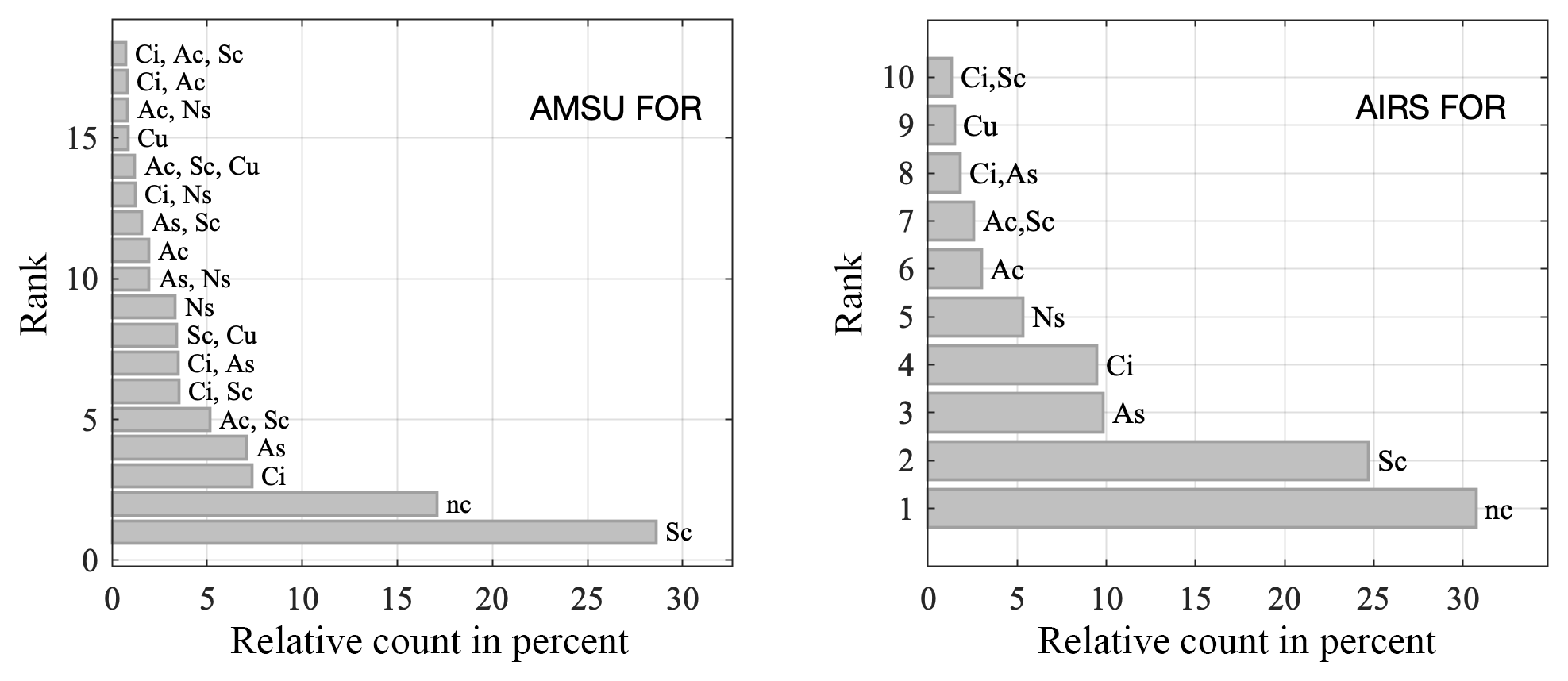
Figure 1Histogram of cloud scenes containing relative counts of occurrence observed at the AMSU FOR and AIRS FOV resolution (∼45 and ∼15 km respectively). The cumulative sum of the relative counts of these 18 (10) cloud scenes amounts to more than 90 % of all cloud scenes observed globally over a period of 2 years at AMSU (AIRS) resolution.
3.1 Cloud scenes with ∼45 km resolution
A cloud scene is assigned to every AMSU FOR along the CloudSat viewing path using the methodology outlined in Sect. 2. Using the 2 years of data, a total of 194 out of 256 possible cloud scenes are observed but only 18 of the cloud scenes account for 90 % of all observed scenes (Fig. 1a). The four most common scenes contain one cloud type with or without clear sky, and the most common mixed cloud scene (Ac, Sc) is ranked as the fifth most common scene overall. Intuitively, the more diverse a scene, the less frequently it should be observed. The scene that ranked last (18th) in Fig. 1a is (Ci, Ac, Sc). The least frequently observed cloud scene with a ranking of 194 contains six cloud types (Ci, As, Ac, St, Cu, Ns) and was observed only once in 2 years. Of the 256 possible types of cloud scenes, the number of unobserved cloud scenes is 62, of which 61 include St. The unobserved cloud scenes include the only possible cloud scene with eight cloud types together and the seven possible cloud scenes with seven cloud types together.
The unobserved scenes in the 2-year period contain a median of five different cloud types. This is consistent with the improbability of particular cloud types occurring in rapid succession over a few tens of kilometers. The only unobserved cloud scene that does not contain St is (Sc, Cu, Ns, Dc) and is consistent with the conclusion by Sassen and Wang (2008) that Dc (1.8 %) and Cu (1.7 %) clouds are the least frequent of the cloud types. While Dc and Ns are typically associated with different climatological regimes (tropical convection versus extratropical storm tracks), occasionally, Dc is embedded within extratropical cyclones and Ns is classified in stratiform regions of mesoscale convective systems (MCSs). Given the prevalence of Sc and Cu in Fig. 1a, it is somewhat surprising that the combination (Sc, Cu, Ns, Dc) is not observed.
The relative ranking of cloud scenes within the AIRS FOV along the CloudSat track is shown in Fig. 1b for the same sets of matched pixels. A total of 10 cloud scenes account for 90 % of all observed cloud scenes (Fig. 1b). This shows that fewer cloud scenes are found at the smaller AIRS FOV compared to the AMSU FOR.
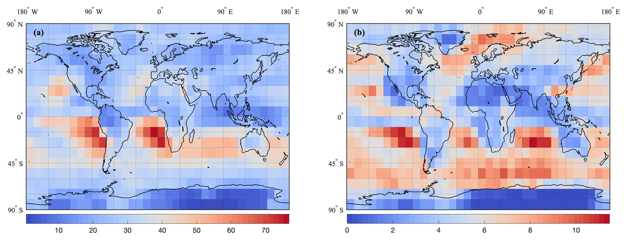
Figure 2Geographic distribution of cloud scenes (Sc) and (Ac, Sc) in panels (a) and (b) respectively, in units of percentage with respect to all of the (194) observed cloud scenes. These scenes were observed at the AMSU FOR resolution (∼45 km). Similar plots of the AIRS FOV resolution (∼15 km) are nearly identical (not shown).
Figure 2 depicts the geographic distribution of Sc at the AMSU FOR scale, the most observed scene after clear sky (nc), and (Ac, Sc) is the most observed mixed cloud scene. The Sc classification is consistent with the prevalence of stratocumulus clouds in subtropical subsidence regions and trade cumulus in the tropics and subtropics (e.g., Yue et al., 2011). The (Ac, Sc) cloud scene is identified most frequently in the extratropical storm tracks and the transition from shallow cumulus to deep tropical convection.
3.2 Cloud scenes at 1 to 1000 km scales
In Sect. 3.1, the relative frequencies of cloud scenes were derived for exact collocated matches of AIRS and AMSU observations to the CloudSat ground track. As the CloudSat ground track can oscillate across several AIRS FOVs over a scan line within a given orbit, the numbers of coincident CloudSat profiles matching to AIRS and AMSU will vary. Below, cloud scenes are derived independently of the specific AIRS and AMSU collocation geometry.
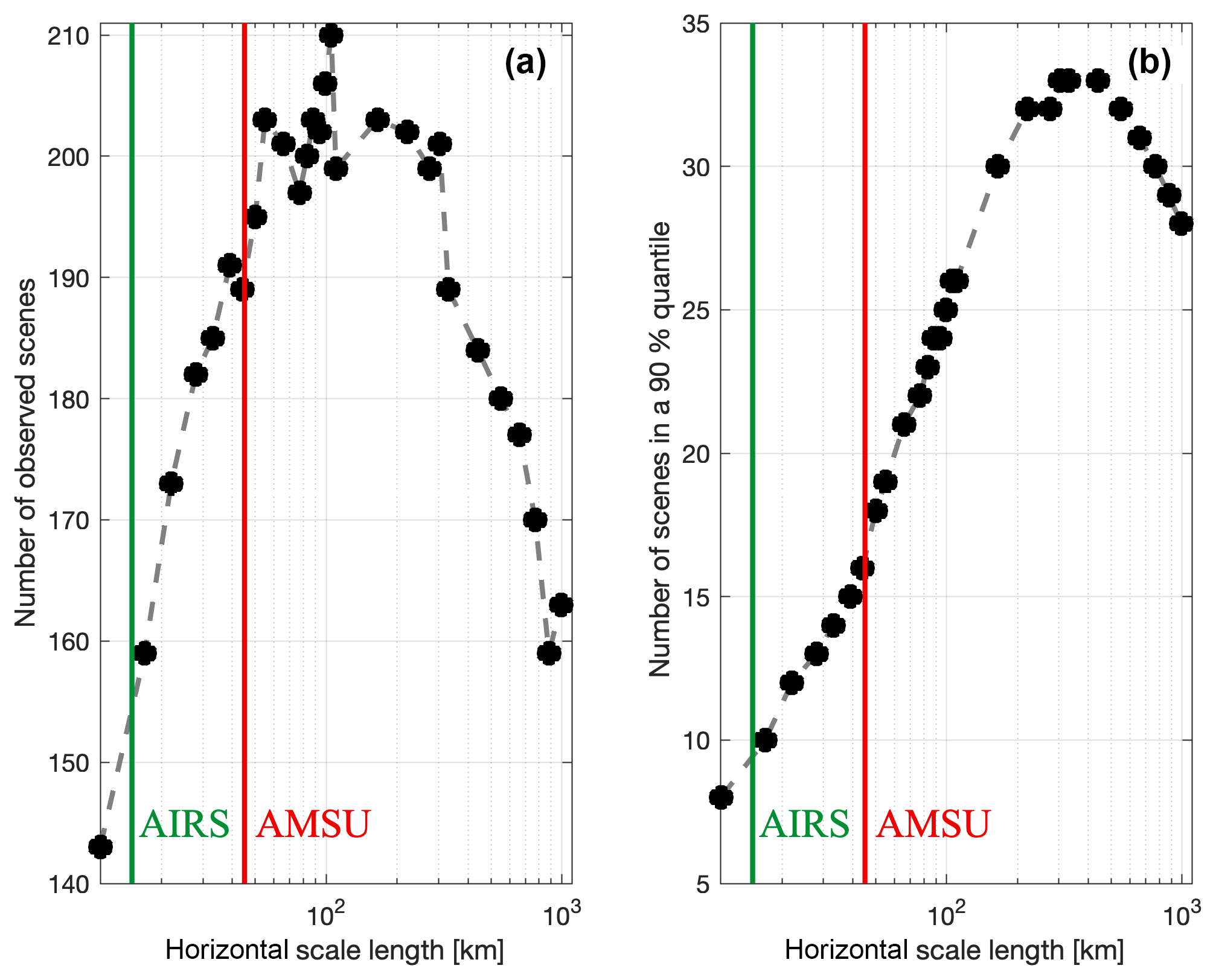
Figure 3(a) Number of observed scenes as a function of the horizontal length scale used to define the scene. (b) Number of scenes observed at the 90th percentile as a function of horizontal length scale used to define the scene. The vertical green (red) lines approximate the scale of the AIRS (AMSU) pixel size.
To investigate the scale dependence of the number of cloud scenes, the approach described in Sect. 2 is modified for a range of horizontal extents between 1.1 and 1000 km. The number of observed cloud scenes calculated at each horizontal scale is shown in Fig. 3a for 10 to 1000 km. At the finest scale of 1.1 km, only eight possible observed cloud scenes or clear sky are expected. When the scale increases, as expected, the number of cloud scenes quickly increases with a total of 143 cloud scenes observed at a scale of 11 km. As horizontal scale is further increased, the probability of observing cloud scenes with only one or two cloud types is reduced. After a maximum number of cloud scenes is obtained at 105 km, the number of cloud scenes will decrease with increasing scale (e.g., 163 cloud scenes at 990 km) until a limiting case is reached at the largest scale with only one cloud scene with all observed cloud types. The number of cloud scenes observed at least once at the AMSU FOR horizontal scale (indicated by the red vertical line on Fig. 3a) is approximately 190.
The 90th percentile calculated at all horizontal scales is shown in Fig. 3b. The 90th percentile of the maximum number of cloud scenes is 33 between 303 and 440 km in horizontal scale. The number at the nominal 45 km AMSU footprint scale is 16 cloud scenes, while the average number at the AIRS footprint is 9 cloud scenes. (Note that these are slightly smaller than values of 18 and 10 using the exact AMSU and AIRS geometry, respectively, in Sect. 3.1.) While these results show that fewer cloud type mixtures are observed at a decreasing length of 45 to 15 km, a variety of cloud type mixtures is still encountered. While infrared sounding at 15 km resolution does not eliminate the cloud scene complexity encountered for combined infrared and microwave sounding at 45 km, the vast majority of 15 km footprints contain a smaller subset of possible cloud mixtures. In Sect. 4, we will determine whether individual cloud types or cloud type mixtures have meaningful impacts on AIRS cloud property retrievals. (Impacts on temperature and specific humidity soundings are beyond the scope of this investigation.)
The reasons for the maximum number of observed cloud scenes (210) at a particular horizontal scale (105 km) are not immediately clear. The scale preference depends on the physical characteristics of cloud regimes and the degree to which cloud types are mixed together by region and furthermore depend on cloud length distributions (Guillaume et al., 2018). A simple model is described below that is able to approximate the results of Fig. 3 and offers some insight for the observed maximum frequency of cloud scenes and the spatial scale at which it occurs.
3.3 Generalizing to all scales
The goal of this section is to derive cloud scene scale statistics that are independent of any regular grid resolution and explore whether these statistics can explain some features of the number of scenes as a function of scale observed in the previous section. In particular, we explore whether these statistics can explain the maximum observed around 105 km. There is however an inherent difficulty in defining the boundaries that delimit any given cloud scene in the absence of a predefined horizontal extent. It is possible that within a given cloud scene there exists several scenes with the same cloud types but differing lengths making the scene identification ambiguous. To circumvent this problem, we define a cloud scene and its maximum length as follows.
-
We search for a cloud scene containing a predefined mixture of cloud types. The spatial extent of this scene is delimited by cloud types (or clear sky) on both ends that do not belong to the mixture.
-
The maximum length of a cloud scene is the sum of all the horizontal lengths of all the cloud types in the cloud scene.
For example, imagine that we will calculate the maximum length of the specific cloud scene (Ac, Sc). We then identify a location in the CloudSat data record with the following illustrative succession of cloud types: (Ci, Ac, Sc, Ac, Sc, Ac, Ns), with the number of CloudSat profiles associated with each cloud type of 10, 3, 6, 5, 7, 12, and 15, respectively. The Ci and Ns obviously do not belong to the (Ac, Sc) cloud scene and therefore delimit the scene as defined in (1) above. The maximum length of the cloud scene (Ac, Sc) will be the sum of the number of CloudSat profiles for (Ac, Sc, Ac, Sc, Ac), which is CloudSat profiles in total. Below, we define a minimum cloud length that is unequivocal.
- 3.
If within a given cloud scene there exist several cloud scenes with the same cloud types but smaller lengths than the maximum length, the minimum length of a cloud scene is defined as the smallest length of all those lengths.
In the example above, there are four possible sequences that could be the minimum length: (Ac, Sc, …, …, …), (…, Sc, Ac, …, …), (…, …, Ac, Sc, …), or (…, …, …, Sc, Ac). The corresponding lengths are , , , and , respectively. In this example, the minimum length would therefore be nine CloudSat profiles. (The minimum and maximum may be equal for a particular mixed cloud scene.)
Before steps (1) and (2) are used to quantify the maximum and minimum lengths for each of the 247 mixed scenes (256 minus the 8 single cloud scenes and clear sky), the locations of each cloud scene must first be identified in the 2-year data record. Starting at the first CloudSat profile, the presence of each of the 247 mixed cloud scenes is determined using (1). For each occurrence of each mixed cloud scene, (2) and (3) are then applied to determine the maximum and minimum lengths for each individual cloud scene. After processing the maximum and minimum lengths for every mixed cloud scene, simple statistics are calculated.
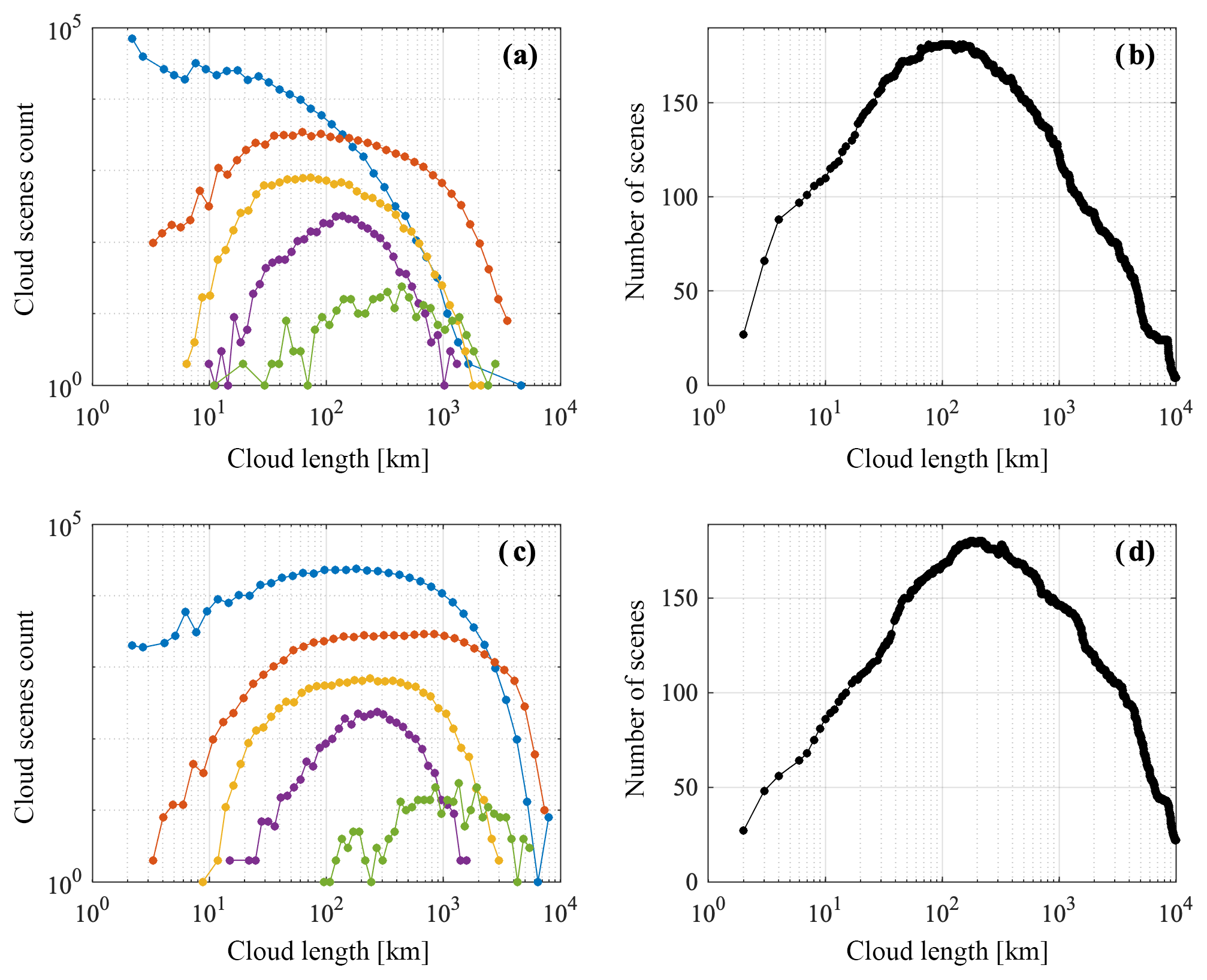
Figure 4Distribution of (a) minimum and (c) maximum length for 5 of the first 200 cloud scenes. The five scenes are, from top to bottom, (Ac, Sc) in blue, (As, Sc, Cu) in orange, (Ci, As, Cu, Dc) in yellow, (As, Ac, Ns, Dc) in purple, and (Ci, As, Ac, St, Sc) in green, and their respective ranks are 1, 26, 51, 76, and 101. In panels (b) and (d), the number of scenes were obtained by summing the number of scenes present a different lengths.
A total of 200 out of 247 possible mixed scenes were identified. The minimum and maximum length occurrence frequencies of five cloud scenes – (Ac, Sc), (As, Sc, Cu), (Ci, As, Cu, Dc), (As, Ac, Ns, Dc), and (Ci, As, Ac, St, Sc) – selected randomly from the 200 present in the 2-year record are shown in Fig. 4a and c, respectively. Recall that the maximum length is defined from (2), while the minimum length is defined from (3), with an illustrative example previously described for (Ac, Sc). From top to bottom, their respective ranks are 1, 26, 51, 76, and 101. It is striking that each frequency histogram in Fig. 4a and c is not monotonic and displays a frequency maximum between 100 and 1000 km. Consequently, the sum of all (200) observed mixed scenes across length scales will result in a curve with a maximum, and these are shown in Fig. 4b and d. Both curves are very similar to Fig. 3a and have maxima for about 180 observed scenes at 77 and 174 km, respectively. Using the methodology outlined in (1) to (3) to estimate numbers of cloud scenes, the scale dependence of the number of observed scenes shows that the maximum will occur somewhere between 77 and 174 km.
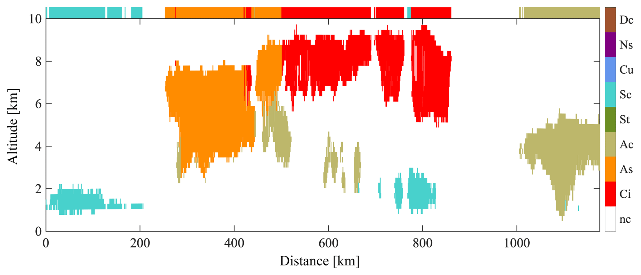
Figure 5Cloud type vertical cross section defined by the values of the cloud_scenario variables of the 2B-CLDCLASS product. Each color corresponds to a different cloud type (legend on right). Color segments on top of the figure indicate the horizontal extent of a cloud measured at its top.
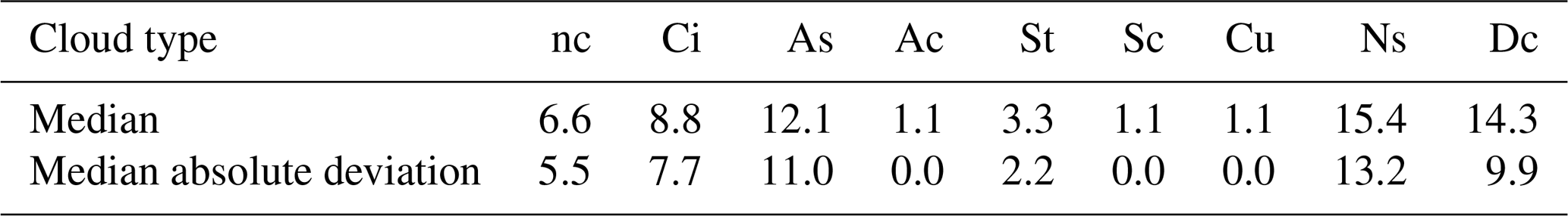
In order to shed additional light on why a maximum in the occurrence frequency of each cloud scene histogram is obtained, histograms of cloud length frequency of single cloud types (defined at cloud top) are calculated. An example CloudSat orbital segment is shown in Fig. 5. The distribution of lengths for each cloud type for the 2-year period is then shown in Fig. 6 with corresponding median and median absolute deviation (or m.a.d.) values reported in Table 1. Note that these values are similar to but not exactly the same as those calculated in Guillaume et al. (2018), for which cloud length was derived from a 2-D curtain of cloud features. The main characteristic shared by all cloud types in Fig. 6 is that their distributions are heavily skewed towards small lengths.
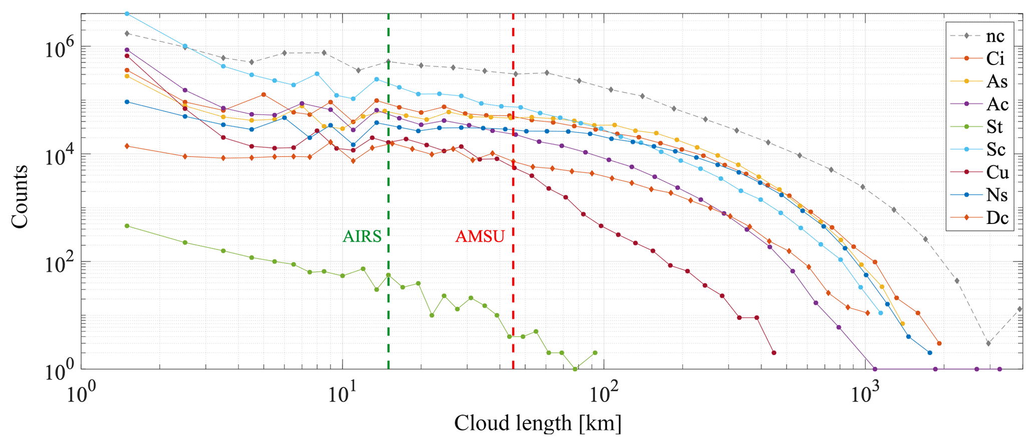
Figure 6Horizontal cloud chord length frequency histograms for each of the eight CloudSat cloud types and clear sky. The cloud chord length was obtained at the cloud top (see Fig. 5) unlike that obtained in Guillaume et al. (2018).
The length of a mixed scene is the sum of the lengths of each cloud type within it. There are two aspects that will influence the number of scenes observed at a given length L. First, there are several combinations of different lengths that will sum to L and those lengths will be smaller than L (abscissa of Fig. 6). Second, the likelihood of observing a given scene depends on the frequency of occurrence of each cloud type (ordinate axis of Fig. 6). These two effects have opposite behaviors as a function of L: single cloud frequency decreases with L, whereas the number of cloud length combinations that sum up to L increases with length scale.
To illustrate the effects of these opposing behaviors, we consider the scene (As, Sc, Cu) length distribution. Since the minimum length of all cloud distributions in Fig. 6 is one CloudSat profile, there is only one possible cloud length combination () that will sum to the minimum possible length of the scene (As, Sc, Cu). This is indeed the value observed on the far left of each red-orange curve in Fig. 4a and c. Next, consider a measurement consisting of four CloudSat profiles with this particular scene, with three possible length combinations: (), (), or (). The frequency of each individual cloud type, As, Sc, or Cu, is smaller at the scale of four CloudSat profiles than it is at a length of three CloudSat profiles in Fig. 6. However, there are more (As, Sc, Cu) scenes at length 4 than at 3 in Fig. 4a and c. This indicates that the increase in possible combinations is more important than the individual cloud frequency decrease for larger scales. This reasoning applies for increasing lengths until the decreasing frequency of individual cloud types between two consecutive lengths is more important. There are very few single As, Sc, or Cu clouds observed at large lengths (far right scale of Fig. 6) resulting in a very small number of observed (As, Sc, Cu) scenes in Fig. 4a and c, despite the large number of length combination possibilities that may contribute.
We will now establish differences in the AIRS thermodynamic-phase and ice cloud properties in the presence of complex and simple cloud types using coincident cloud scenes. In this section, the scenes are determined at the AIRS FOV resolution (approximately 15 km). We briefly summarize general categories of cloud scene statistics in Sect. 4.1. The AIRS cloud-thermodynamic-phase tests are discussed separately for single and mixed cloud scenes in Sect. 4.2. The AIRS ice cloud τi and rei, error estimates, averaging kernels (i.e., information content), and χ2 residual fits between observed and simulated radiances are shown in Sect. 4.3.
Table 1Horizontal cloud chord length median and median absolute deviation for each cloud type (km).
4.1 Types of cloud scenes
Table 2 summarizes five types of scenes at the 15 km AIRS FOV scale: (i) clear sky, (ii) cloudy sky with one cloud type, (iii) partly cloudy sky with one cloud type, (iv), cloudy sky with multiple cloud types, and (v) partly cloudy sky with multiple cloud types. The raw counts and the relative percentages for the 2-year observing period are shown. The dominance of clear sky (30.7 %) at 15 km is apparent and is consistent with an absence of thin cloud features in the 2B-CLDCLASS data set. Cloudy sky scenes with one cloud type (multiple cloud types) amount to 31.3 % (10.2 %) of all observed scenes, while partly cloudy sky scenes with one cloud type (multiple cloud types) amount to 23.5 % (4.3 %) of all observed scenes. A total of 41.5 % of AIRS FOVs are completely cloudy while 27.8 % are partly cloudy according to 2B-CLDCLASS. Below the differences in cloud-thermodynamic-phase detection and ice cloud property retrievals are quantified for the types of scenes summarized in Table 2.
4.2 Cloud thermodynamic phase
The occurrence frequency histogram of the sum of all thermodynamic-phase tests is shown for cloudy sky with one cloud type in Fig. 7. Homogeneous cloud scenes serve as an ideal point of reference for establishing cloud-phase sensitivity benchmarks. Overall, there is strong differentiation in the cloud thermodynamic phase among cloud scenes with single cloud types. Ice tests dominate Ci, Ns, Dc, and As, while liquid and undetermined tests dominate Ac, Sc, and Cu.
The ice tests dominate the Ci cloud scenes and reaffirm the sensitivity of AIRS to ice clouds. CloudSat-classified clear scenes contain occasional occurrences of AIRS-detected thin cirrus (+1 and +2), consistent with either thin cirrus that is undetected by the CloudSat radar or thicker cirrus within the AIRS footprint but to the side of the CloudSat ground track (e.g., Kahn et al., 2008). A few occurrences of −1 and −2 may also arise from spatial mismatches between AIRS and CloudSat scenes, or from stratus below 1 km in altitude that is undetected by CloudSat. In the Sc cloud scenes, trade cumulus clouds dominate as previously shown by Yue et al. (2011) and Kahn et al. (2017). A larger proportion of liquid tests, and a smaller proportion of ice tests, is observed in the Sc cloud scenes compared to clear sky, but undetermined phase is dominant in both scene types. The Cu and Sc cloud scene histograms are generally similar with more undetermined cases for Cu, but with a slight reduction of liquid and slight increase in ice observed for Cu compared to Sc.

Figure 7AIRS cloud_phase_3x3 histograms for cloudy sky with one cloud type (i.e., all CloudSat profiles have the same cloud type and no clear sky). The red, green, and blue bars indicate liquid, undetermined, and ice phase, respectively. Each histogram sums to 1.0 and does not show how many counts relative to another histogram. Relative counts could be inferred from the percentages listed in the second to left column of Table 3.
The As cloud scene histogram in Fig. 7 is overwhelmingly dominated by ice. The undetermined cases in part may result from supercooled liquid or mixed-phase clouds that potentially could be distinguished with an improved phase algorithm that factors in the spectral midinfrared signature of supercooled liquid (e.g., Rowe et al., 2013). The Ac and As cloud scene histograms are very different from each other, with a majority of undetermined and liquid for Ac and a majority of ice for As, consistent with aircraft observations (Mazin, 2006). The preponderance of undetermined phase for Ac may indicate frequent supercooled liquid cloud tops (Zhang et al., 2010). Ham et al. (2013) showed that Ac are typically 2–3 km lower in altitude than As, and this probably explains some of the difference in liquid and ice phase, as lower clouds are usually warmer. The Ns cloud scene histogram is dominated by ice detection with occasional liquid and undetermined cloud tops. The Ns cloud scene also has significant height overlap with Ac and As, with most tops for all three types typically located below 9 km. Ice tests dominate in the Dc cloud scene histogram although a very small proportion of −1, 0, and +1 occur. Inspection of AIRS granules (not shown) demonstrates that the spectral signatures used in thermal infrared phase tests break down in the presence of overshooting convection and other ice clouds within a few Kelvin of the tropopause (e.g., Kahn et al., 2018).
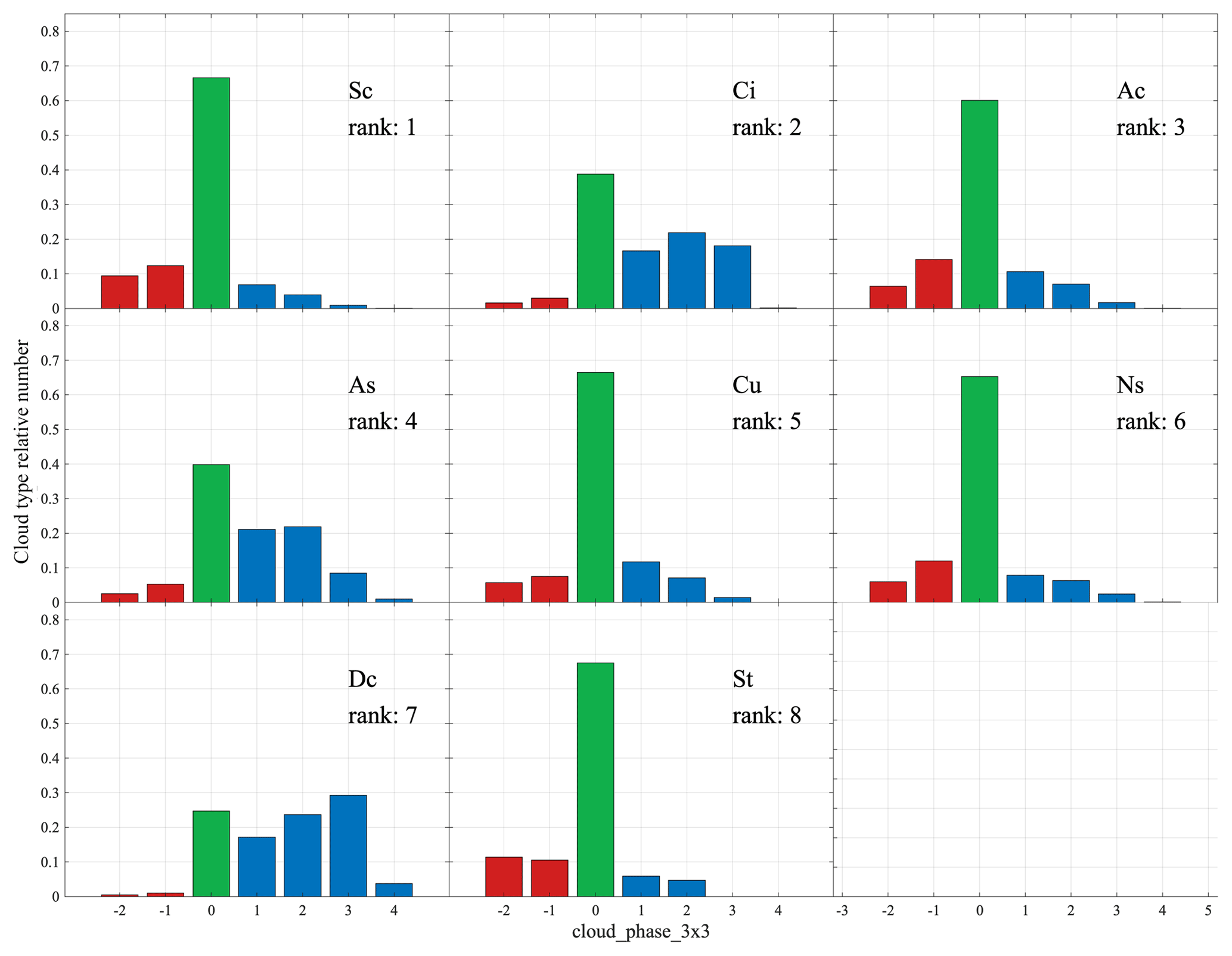
Figure 8AIRS cloud_phase_3x3 histograms for partly cloudy sky with one cloud type. All else equal to Fig. 7.
The occurrence frequencies of cloud phase for partly cloudy sky with one cloud type are shown in Fig. 8. The biggest change is the relative ordering of the ranks among cloud scene types between Figs. 7 and 8. Ac is now more common than As, as horizontal extent and frequency both explain reordering of rankings in Figs. 7 and 8 (Miller et al., 2014; Guillaume et al., 2018). There are more subtle changes in the cloud-phase histograms that are consistent with partly cloudy sky. A weaker spectral signature for partly cloudy scenes results in slightly greater counts of unknown phase and also subtle shifts in liquid- and ice-phase tests in Fig. 8 compared to Fig. 7. In the Ac cloud scene histograms, there is a small but discernible increase in ice tests in Fig. 8 compared to Fig. 7. Horizontally heterogeneous Ac appears to have more frequent ice detection than horizontally homogeneous Ac.
Table 2Total counts and relative percentages of five cloud scene categories at the AIRS FOV scale: clear sky, cloudy sky with one cloud type, partly cloudy sky with one cloud type, cloudy sky with multiple cloud types, and partly cloudy sky with multiple cloud types.

The nine most frequent cloudy scenes with multiple cloud types are shown in Fig. 9. The (Ci, Sc) cloud scene ice-phase histogram resembles a hybrid of histograms for Ci and Sc with undetermined phase the most frequent. (Ci, Sc) is a common cloud scene in the low latitudes as trade cumulus (Sc cloud type) and is frequently found under thin cirrus (Chang and Li, 2005). Furthermore, the spectral signatures of the two types of clouds frequently cancel, giving an undetermined phase result in the spectral tests used here (not shown). The (Ci, As) cloud scene shows a slight reduction in liquid detections and a slight increase in ice detections compared to As alone. While the As cloud scene in Fig. 7 is dominated by +2, the (Ci, As) cloud scene is dominated by +2 and +3. This suggests that a mixture of Ci and As together can trigger more ice tests in AIRS than As alone.
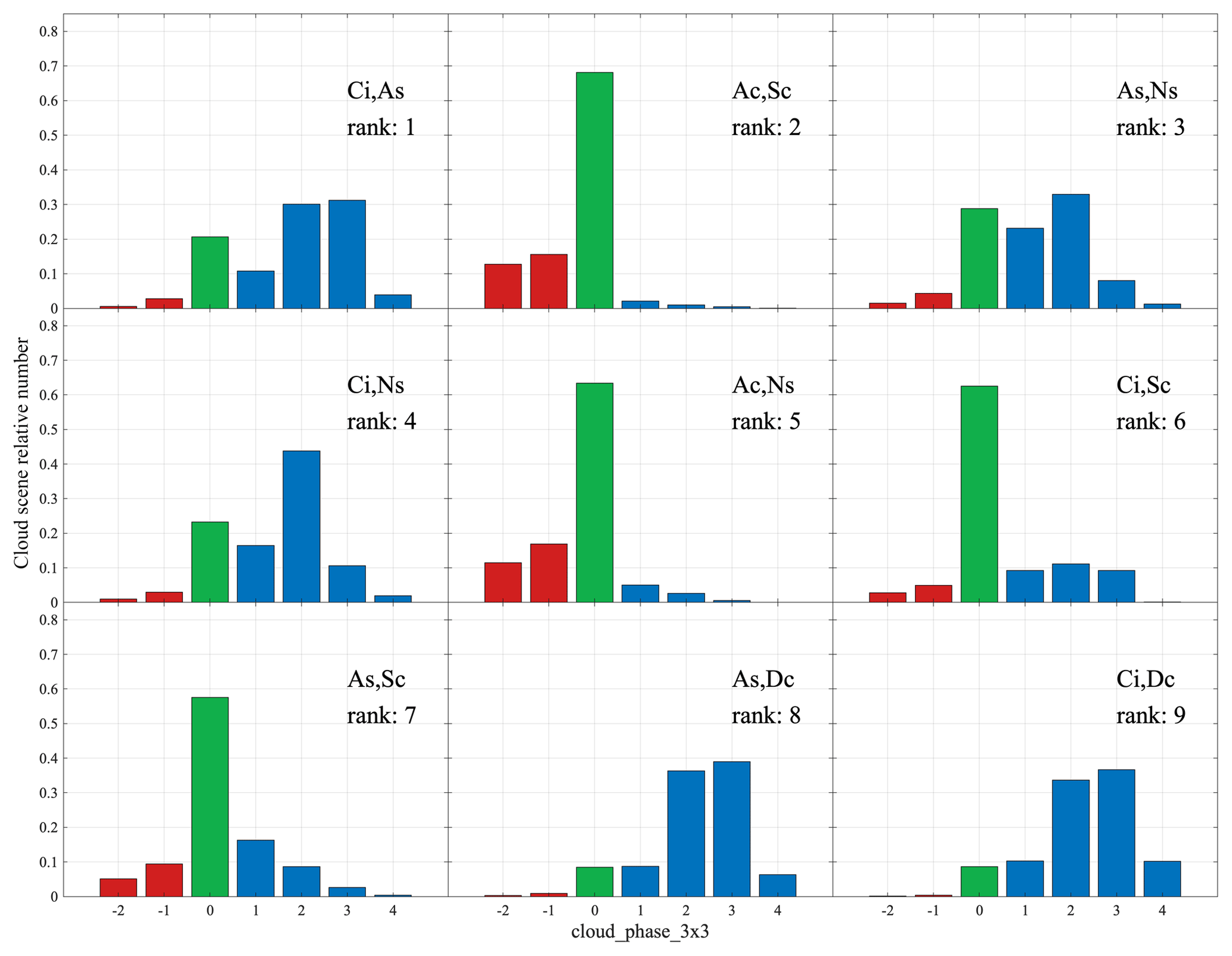
Figure 9AIRS cloud_phase_3x3 histograms for cloudy sky with multiple cloud types for the top nine ranked cloud scenes in order of occurrence frequency.
The nine most frequent partly cloudy scenes with multiple cloud types are shown in Fig. 10. As with the differences between Figs. 7 and 8, the biggest change is the relative ordering of the ranks among cloud scene types between Figs. 9 and 10. Furthermore, there are additional (yet subtle) changes in the phase test histograms for the cloud scenes that are common between Figs. 9 and 10.
In most mixed cloud scenes in both Figs. 9 and 10, the characteristics of the histograms are similar either to single types or have combined characteristics of the multiple cloud types contained within the cloud scene. These results are encouraging and reaffirm the capabilities of thermal-infrared cloud-phase determination (Jin and Nasiri, 2014) and exhibit consistency with cloud types from the CloudSat radar. We note, however, that the AIRS phase determination has some ambiguity in overlapping ice and liquid cloud layers as previously shown by Jin and Nasiri (2014).
Table 3Cloud ice properties for cloudy sky with one cloud type (i.e., all CloudSat profiles have the same cloud type). Proportions and relative errors are in percent. The effective radius is in micrometers (µm).
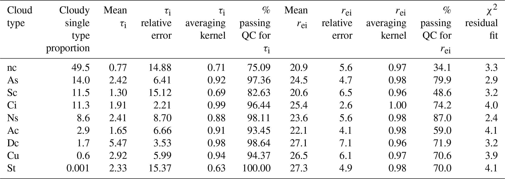
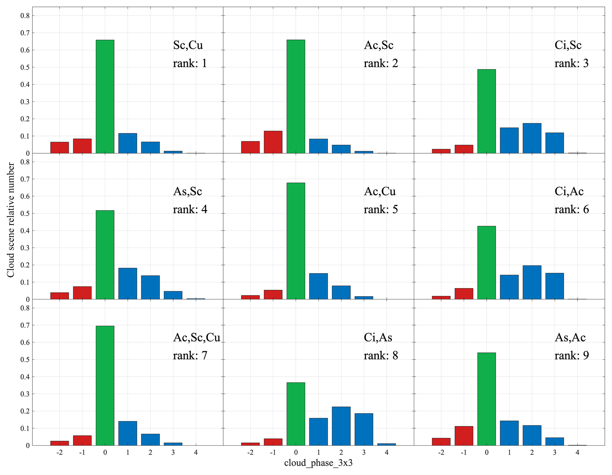
Figure 10AIRS cloud_phase_3x3 histograms for partly cloudy sky with multiple cloud types for the top nine ranked cloud scenes in order of occurrence frequency.
4.3 Ice cloud properties
The mean ice cloud property retrievals are summarized in Table 3 for cloudy sky with one cloud type only for the ice-only portions of the cloud-phase histograms depicted in Fig. 7. Scenes identified as clear sky exhibit properties of a small population of thin cirrus detected by AIRS (Fig. 7) with mean values of τi=0.77 and rei=20.9 µm (Table 3). The AKs are notably lower and the relative error for τi is higher than other cloud scenes. The Sc cloud scene shows a small population of cirrus that go undetected in 2B-CLDCLASS (Fig. 7) and have mean values of τi=1.30 and rei=20.6 µm (Table 3). The AKs are also lowest in Table 3 for Sc relative to other cloud scenes with similarly high errors in τi and rei. Kahn et al. (2008, 2015) have shown that AIRS is very sensitive to thin cirrus; thus some ice clouds in CloudSat-identified Sc cloud scenes are expected. Because tenuous ice clouds have smaller values of τi and rei, the lower estimates of information content and larger error estimates are promising. These tenuous ice cloud retrievals are differentiated well from more robust retrievals within cloud scenes that are dominated by ice phase in the histograms (Fig. 7).
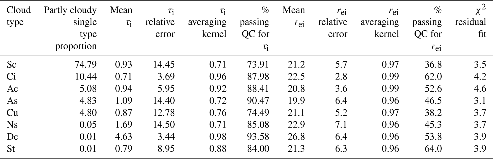
Table 4Cloud ice properties for partly cloudy sky with one cloud type. All else the same as Table 3.
The Ci cloud scene has mean values of τi=1.91 and rei=25.4 µm; an AK =1.0, the highest of any scene type; and lower errors compared to other types in Table 3. The As cloud scene has a larger mean of τi=2.42 compared to the Ac cloud scene with a mean of τi=1.65 (Table 3). Interestingly, the mean value and error estimate of rei is lower for Ac than As, exhibiting differentiation between these two midlevel cloud types. However, a much smaller proportion of Ac is ice compared to As (Fig. 7).
The Ns cloud scene in Table 3 contains larger mean values of τi than Ci and Ac cloud scenes, but these values are similar to those for As; however, the mean values are lower than Cu and Dc cloud scenes (Table 3). A lower value of τi is characteristic of diffuse cloud tops where the infrared emission may originate several kilometers deep within the cloud (e.g., see Kahn et al., 2008; Holz et al., 2006). The reduced AK =0.88 for the Ns cloud scenes illustrates that a diffuse cloud top is more problematic for ice cloud retrievals. Cu cloud scenes with ice cloud tops occur a small amount of the time (Fig. 7); furthermore, Cu is infrequent in CloudSat classification (1.7 % of all clouds). The horizontal extent of Cu is also much smaller than Dc (see Table 1). Interestingly, τi is larger for Cu cloud scenes than for all categories except Dc cloud scenes (Table 2).
The mean Cu value of rei=26.5 µm is larger than most cloud scenes. This is consistent with larger ice particles observed at the tops of convection instead of small ice particles in thin cirrus at the same cloud top temperature (e.g., Yuan and Li, 2010; Protat et al., 2011; van Diedenhoven et al., 2014; Kahn et al., 2018). These Cu cases are likely transient cumulus congestus at altitudes cold enough for cloud top glaciation. The Dc cloud scene has the largest mean τi=5.47 of all cloud scenes with a very dense cloud top that saturates the infrared emission signal in contrast to Ns. The values of rei for Dc are similar to Cu (Table 3), with a slight reduction in the rei AK =0.96 and τi AK =0.98 relative to Ci cloud scenes (Table 3). This is consistent with reduced sensitivity for high values of τi (e.g., Huang et al., 2004).
The relative variations between the ice cloud retrieval properties for cloudy sky with one cloud type in Table 3 are consistent with expectations of infrared sensitivity. CloudSat-observed Ci cloud scenes have smaller error estimates and higher information content in comparison to Sc, consistent with Sc scenes containing tenuous cirrus that goes undetected by 2B-CLDCLASS. Larger τi and rei are observed at the tops of convective ice clouds such as Dc and Cu compared to stratiform clouds such as As and Ci. Differences in ice cloud properties between Ac and As cloud scenes are consistent with observed differences in scene heterogeneity and cloud top height.
The mean ice cloud property retrievals are summarized in Table 4 for partly cloudy sky with one cloud type with cloud-phase histograms depicted in Fig. 8. The biggest difference between Tables 3 and 4 is the relative frequency of occurrence with large differences between cloud scenes with or without clear sky. Another significant change is an overall reduction in AKs and magnitude of τi, with an increase in χ2 in Table 4, consistent with partly cloudy scenes. The changes in rei AKs, magnitudes, and error estimates between Tables 3 and 4 are smaller than those for τi. Overall, the differences between Tables 3 and 4 are reassuring in that the AIRS retrieval is responding to partly cloudy scenes by reducing information content and the magnitude of τi, while χ2 residuals are increasing somewhat.
The As and Ac cloud scenes in Table 4 are very similar to As and Ac cloud scenes in Table 3 except for slight reductions in τi and rei. Scenes in Table 4 are partly cloudy, implying a weaker infrared cloud signal. The Ci cloud scene in Table 4 shows slight reductions in τi and rei from the Ci cloud scene in Table 3.
The differences between Tables 3 and 4 are more significant for the convective ice clouds, however. The Cu cloud scene τi and AK are smaller while errors are larger in Table 4 compared to the pure Cu cloud scene in Table 3. This is expected as Cu clouds are several kilometers in depth but often have small horizontal scales and are averaged with clear sky in an AIRS pixel. Mixed (Cu, Nc) cloud scenes are especially problematic for plane-parallel radiative transfer calculations. This results in more uncertain retrievals of ice cloud properties for partial cloud (Cu, Nc) in Table 3 than those for the pure Cu cases in Table 2, which are more likely to completely fill an AIRS scene.
Table 5Cloud ice properties for cloudy sky with multiple cloud types for the first nine most observed cloud scenes at the AIRS FOV scale. All else the same as Table 4.
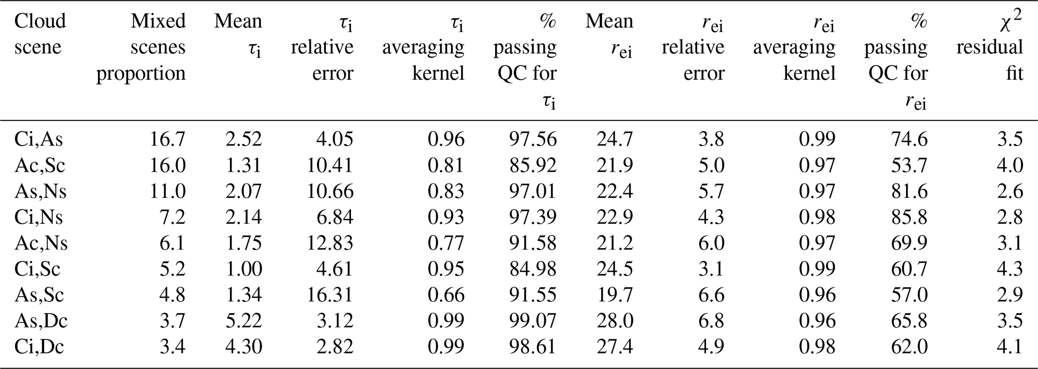
Table 6Cloud ice properties for partly cloudy sky with multiple cloud types for the first nine most observed cloud scenes at the AIRS FOV scale. All else the same as Table 5.
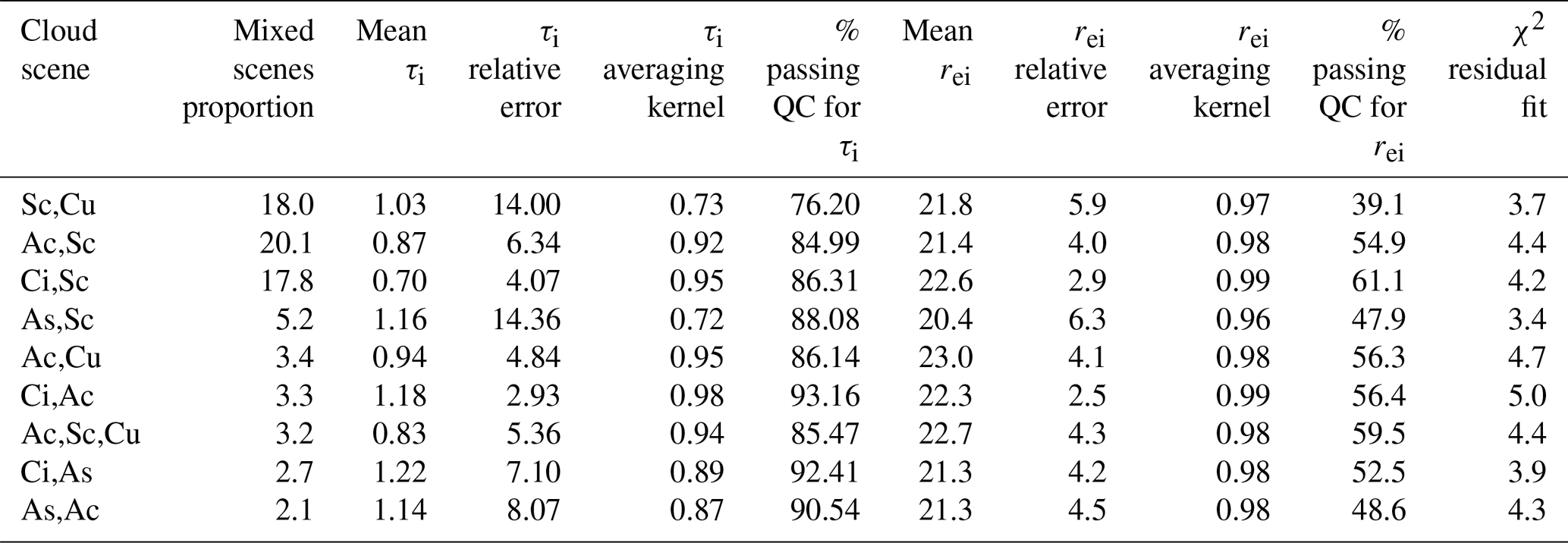
The ice cloud property retrievals for cloud scenes that contain multiple cloud types are summarized in Table 5 for cloudy scenes and Table 6 for partly cloudy scenes. These tables list the nine most frequent cloud scene types as depicted in Figs. 9 and 10. Four of the nine cloud scenes are common between Tables 5 and 6. There is a general tendency for reductions of τi, increases in percent relative error, and slight reductions in AKs in Table 6 for the seven common cloud scenes in Table 5. Changes in rei-related variables are smaller than changes in τi-related variables.
To summarize Tables 3–6, larger differences in ice cloud property retrievals are found between different cloud types than between cloudy and partly cloudy scenes. However, the differences between cloud scene types are the sharpest for the subset of cloudy scenes with one cloud type (Table 3). The AIRS cloud property retrievals are not greatly impacted by mixtures of cloud types within the AIRS footprint, and ice cloud property differences among cloud scenes are broadly consistent with the expected performance of infrared retrievals among these cloud types.
A method is described to classify cloud mixtures of cloud top types, termed cloud scenes, using the 2B-CLDCLASS cloud type classification obtained from the 94 GHz CloudSat radar. The scale dependence of the cloud scenes is quantified. The method is initially applied to 2 years of CloudSat data collocated within the Atmospheric Infrared Sounder (AIRS)/Atmospheric Microwave Sounding Unit (AMSU) field of regard (FOR) at a 45 km scale. Given the 45 km scale and approximately 50 coinciding CloudSat profiles, each with 125 levels, the total number of possible scenes within an AMSU FOR is 950×125. This very large number of possible scenes is reduced to 256 by making three assumptions in the classification. First, only the cloud type at the cloud top is considered. Second, the occurrence frequency of each cloud type within the cloud scene is disregarded; thus, there is no consideration of the counts of each cloud type. Third, the sequence of cloud types along the orbit segment is not considered. These three assumptions make mixed cloud scene classification tractable and are broadly consistent with the sensitivity of infrared sounders to clouds. They are also independent of the spatial scale of a scene and therefore can be generalized to all horizontal scales. A total of 210 out of 256 possible cloud scenes are observed in a 2-year period from 1 July 2006 to 30 June 2008. The maximum number of cloud scenes occurs at a horizontal scale of 105 km with fewer cloud scenes at larger and smaller scales, and the majority of observed cloud scenes contain single cloud types.
The cloud scenes are organized into five categories: (i) clear sky, (ii) cloudy sky with one cloud type, (iii) partly cloudy sky with one cloud type, (iv), cloudy sky with multiple cloud types, and (v) partly cloudy sky with multiple cloud types. Summarizing AIRS cloud top property retrievals for cloudy sky with one cloud type, there is strong differentiation in the cloud thermodynamic phase. Ice phase dominates Ci, Ns, Dc, and As, while liquid and undetermined phase dominate Ac, Sc, and Cu. The results are similar for partly cloudy sky with one cloud type with an increase in unknown cloud phase and χ2 residuals, as well as a reduction in information content for some cloud types. A similar set of calculations were performed for both cloudy and partly cloudy skies with multiple cloud types. In most cloud scenes with multiple cloud types, the changes in the ice properties are generally either small or reflect the combined characteristics of the multiple cloud types contained within the cloud scene. The sensitivity of thermal infrared cloud-phase determination is consistent with independently determined cloud typing from the CloudSat radar for clouds detected by CloudSat.
The relative magnitude of differences in rei and τi, and their averaging kernels (AKs) and error estimates, and the χ2 residual between simulated and observed radiances are consistent with expectations of infrared retrieval sensitivity to different cloud types. Smaller error estimates and higher information content (AKs) within Ci cloud scenes are observed in comparison to thin cirrus likely missed by CloudSat in clear sky and Sc scenes. Larger τi and rei are observed at the tops of convective ice clouds. Differences in retrieved cloud properties between Ac and As cloud scenes are consistent with differences in their scene heterogeneity and cloud temperature. Variations in ice cloud property retrievals are larger between types of cloud scenes than between cloudy and partly cloudy/mixed cloud scenes.
The fidelity of AIRS-retrieved cloud-phase and ice cloud microphysics was tested within scenes with both uniform and nonuniform cloud cover, as well as one or more cloud types within the scene. As with phase, retrieval differences are shown to be larger among cloud types rather than between uniform and mixed cloud scenes.
New methodologies for simultaneous retrievals of cloud microphysical properties and temperature and specific humidity profiles that include clouds in the forward radiative transfer (e.g., De Souza-Machado et al., 2018; Irion et al., 2018) necessitate careful investigation of the effects of cloud mixtures on retrieved cloud properties. The bias and root-mean square error of AIRS temperature and specific humidity soundings depend on cloud type (Yue et al., 2013; Wong et al., 2015). A more rigorous evaluation of scene complexity is necessary for optimizing the retrieval configuration of future sounding algorithms (Irion et al., 2018) and for validating their products.
This investigation shows that careful inspection of footprint-scale AIRS cloud property retrievals is consistent with expectations of infrared sensitivity to different cloud types defined with the 94 GHz CloudSat radar. Other cloud observations, such as MODIS, may be used in a similar analysis to the one described here. MODIS captures the off-nadir portion of the AIRS swath and the fine-scale variability within AIRS footprints. Wang et al. (2016) used the cloud typing in CloudSat to cross validate with cloud typing using MODIS-defined cloud types. This establishes a link between cloud types obtained from CloudSat and MODIS. A rigorous estimation of the pixel-scale relationships between cloud properties obtained from CloudSat, MODIS, and AMSU will help to further advance multisensor and multivariate geophysical retrievals (e.g., Irion et al., 2018).
CloudSat data were obtained through the CloudSat Data Processing Center (http://www.cloudsat.cira.colostate.edu/, Cooperative Institute, 2019). The combined data files used in this work are available at the Goddard Earth Sciences Data and Information Services Center (Fetzer at al., 2013).
AG designed and implemented the cloud scene classification scheme as well as the cloud scene and cloud type scale dependence studies. BK designed and AG implemented the study of AIRS thermodynamic-phase and ice cloud properties as a function of cloud scenes and types. GM designed, implemented, and generated the AIRS/AMSU/CloudSat matchup product. GM, BW, and HH designed the data system that generated this product. AG and BK prepared the manuscript with contributions from all coauthors.
The authors declare that they have no conflict of interest.
Part of this research was carried out at the Jet Propulsion Laboratory (JPL), California Institute of Technology, under a contract with the National Aeronautics and Space Administration. The authors thank two reviewers for helpful and insightful comments that led to an improved manuscript. This project was supported by NASA's Making Earth Science Data Records for Use in Research Environments (MEaSUREs) program.
This research has been supported by NASA (grant no. NNH17ZDA001N).
This paper was edited by Alexander Kokhanovsky and reviewed by two anonymous referees.
Barnes, E. A. and Polvani, L.: Response of the Midlatitude Jets, and of Their Variability, to Increased Greenhouse Gases in the CMIP5 Models, J. Climate, 26, 7117–7135, 2013.
Bony, S., Colman, R., Kattsov, V. M., Allan, R. P., Bretherton, C. S., Dufresne, J.-L., Hall, A., Hallegatte, S., Holland, M. M., Ingram, W., Randall, D. A., Soden, B. J., Tselioudis, G., and Webb, M. J.: How Well Do We Understand and Evaluate Climate Change Feedback Processes?, J. Climate, 19, 3445–3482, 2006.
Ceppi, P., Hartmann, D. L., and Webb, M. J.: Mechanisms of the Negative Shortwave Cloud Feedback in Middle to High Latitudes, J. Climate, 29, 139–157, 2016.
Chahine, M. T., Pagano, T. S., Aumann, H. H., Atlas, R., Barnet, C., Blaisdell, J., Chen, L., Divakarla, M., Fetzer, E. J., Goldberg, M., Gautier, C., Granger, S., Hannon, S., Irion, F. W., Kakar, R., Kalnay, E., Lambrigtsen, B. H., Lee, S., Le Marshall, J., Mcmillan, W. W., Mcmillin, L., Olsen, E. T., Revercomb, H., Rosenkranz, P., Smith, W. L., Staelin, D., Strow, L. L., Susskind, J., Tobin, D., Wolf, W., and Zhou, L.: The Atmospheric Infrared Sounder (AIRS): Improving weather forecasting and providing new insights into climate, B. Am. Meteorol. Soc., 87, 911–926, https://doi.org/10.1175/BAMS-87-7-911, 2006.
Chang, F. L. and Li, Z.: A near global climatology of single-layer and overlapped clouds and their optical properties retrieved from TERRA/MODIS data using a new algorithm, J. Climate, 18, 4752–4771, 2005.
Cooperative Institute for Research in the Atmosphere, Colorado State University, CloudSat Data Processing Center, available at: http://www.cloudsat.cira.colostate.edu/, last access: 8 August 2019.
DeSouza-Machado, S., Strow, L. L., Tangborn, A., Huang, X., Chen, X., Liu, X., Wu, W., and Yang, Q.: Single-footprint retrievals for AIRS using a fast TwoSlab cloud-representation model and the SARTA all-sky infrared radiative transfer algorithm, Atmos. Meas. Tech., 11, 529–550, https://doi.org/10.5194/amt-11-529-2018, 2018.
Fetzer, E., Wilson, B., and Manipon, G.: AIRS-CloudSat cloud mask, radar reflectivities, and cloud classification matchups V3.2, Greenbelt, MD, USA, Goddard Earth Sciences Data and Information Services Center (GES DISC), https://doi.org/10.5067/MEASURES/WVCC/DATA203, 2013.
Golaz, J.-C., Larson, V. E., and Cotton, W. R.: A PDF-Based Model for Boundary Layer Clouds. Part I: Method and Model Description, J. Atmos. Sci., 59, 3540–3551, 2002.
Guillaume, A., Kahn, B. H., Yue, Q., Fetzer, E. J., Wong, S., Manipon, G. J., Hua, H., and Wilson, B. D.: Horizontal and vertical scaling of cloud geometry inferred from CloudSat data, J. Atmos. Sci., 75, 2187–2197, https://doi.org/10.1175/JAS-D-17-0111.1, 2018.
Ham, S.-H., Sohn, B.-J., Kato, S., and Satoh, M.: Vertical structure of ice cloud layers from CloudSat and CALIPSO measurements and comparison to NICAM simulations, J. Geophys. Res.-Atmos., 118, 9930–9947, https://doi.org/10.1002/jgrd.50582, 2013.
Holz, R. E., Ackerman, S., Antonelli, P., Nagle, F., Knuteson, R. O., McGill, M., Hlavka, D. L., and Hart, W. D.: An improvement to the high spectral resolution CO2 slicing cloud top altitude retrieval, J. Atmos. Ocean. Tech., 23, 653–670, 2006.
Huang, H.-L., Yang, P., Wei, H., Baum, B. A., Hu, Y., Antonelli, P., and Ackerman, S. A.: Inference of ice cloud properties from high spectral resolution infrared observations, IEEE T. Geosci. Remote, 42, 842–853, 2004.
Irion, F. W., Kahn, B. H., Schreier, M. M., Fetzer, E. J., Fishbein, E., Fu, D., Kalmus, P., Wilson, R. C., Wong, S., and Yue, Q.: Single-footprint retrievals of temperature, water vapor and cloud properties from AIRS, Atmos. Meas. Tech., 11, 971–995, https://doi.org/10.5194/amt-11-971-2018, 2018.
Jakob, C. and Tselioudis, G.: Objective identification of cloud regimes in the Tropical Western Pacific, Geophys. Res. Lett., 30, 2082, https://doi.org/10.1029/2003GL018367, 2003.
Jin, H. and Nasiri, S. L.: Evaluation of AIRS cloud-thermodynamic-phase determination with CALIPSO, J. Appl. Meteorol. Clim., 53, 1012–1026, 2014.
Kahn, B. H., Chahine, M. T., Stephens, G. L., Mace, G. G., Marchand, R. T., Wang, Z., Barnet, C. D., Eldering, A., Holz, R. E., Kuehn, R. E., and Vane, D. G.: Cloud type comparisons of AIRS, CloudSat, and CALIPSO cloud height and amount, Atmos. Chem. Phys., 8, 1231–1248, https://doi.org/10.5194/acp-8-1231-2008, 2008.
Kahn, B. H., Irion, F. W., Dang, V. T., Manning, E. M., Nasiri, S. L., Naud, C. M., Blaisdell, J. M., Schreier, M. M., Yue, Q., Bowman, K. W., Fetzer, E. J., Hulley, G. C., Liou, K. N., Lubin, D., Ou, S. C., Susskind, J., Takano, Y., Tian, B., and Worden, J. R.: The Atmospheric Infrared Sounder version 6 cloud products, Atmos. Chem. Phys., 14, 399–426, https://doi.org/10.5194/acp-14-399-2014, 2014.
Kahn, B. H., Schreier, M. M., Yue, Q., Fetzer, E. J., Irion, F. W., Platnick, S., Wang, C., Nasiri, S. L., and L'Ecuyer, T. S.: Pixel-scale assessment and uncertainty analysis of AIRS and MODIS ice cloud optical thickness and effective radius, J. Geophys. Res.-Atmos., 120, 11669–11689, https://doi.org/10.1002/2015JD023950, 2015.
Kahn, B. H., Matheou, G., Yue, Q., Fauchez, T., Fetzer, E. J., Lebsock, M., Martins, J., Schreier, M. M., Suzuki, K., and Teixeira, J.: An A-train and MERRA view of cloud, thermodynamic, and dynamic variability within the subtropical marine boundary layer, Atmos. Chem. Phys., 17, 9451–9468, https://doi.org/10.5194/acp-17-9451-2017, 2017.
Kahn, B. H., Takahashi, H., Stephens, G. L., Yue, Q., Delanoë, J., Manipon, G., Manning, E. M., and Heymsfield, A. J.: Ice cloud microphysical trends observed by the Atmospheric Infrared Sounder, Atmos. Chem. Phys., 18, 10715–10739, https://doi.org/10.5194/acp-18-10715-2018, 2018.
Klein, S. A. and Jakob, C.: Validation and Sensitivities of Frontal Clouds Simulated by the ECMWF Model, Mon. Weather Rev., 127, 2514–2531, 1999.
Krijger, J. M., van Weele, M., Aben, I., and Frey, R.: Technical Note: The effect of sensor resolution on the number of cloud-free observations from space, Atmos. Chem. Phys., 7, 2881–2891, https://doi.org/10.5194/acp-7-2881-2007, 2007.
Manipon, G.: README document for A Multi-Sensor Water Vapor Climate Data Record Using Cloud Classification, 32 pp., available at: https://docserver.gesdisc.eosdis.nasa.gov/public/project/MEaSUREs/Fetzer/README.AIRS_CloudSat.pdf (last access: 8 August 2019), 2016.
Mazin, I. P.: Cloud phase structure: Experimental data analysis and parameterization, J. Atmos. Sci., 63, 667–681, 2016.
Miller, S. D., Forsythe, J. M., Partain, P. T., Haynes, J. M., Bankert, R. L., Sengupta, M., Mitrescu, C., Hawkins, J. D., and Vonder Haar, T. H.: Estimating three-dimensional cloud structure via statistically blended satellite observations, J. Appl. Meteorol. Clim., 53, 437–455, https://doi.org/10.1175/JAMC-D-13-070.1, 2014.
Mitchell, J. F. B., Senior, C. A., and Ingram, W. J.: CO2 and climate: A missing feedback?, Nature, 341, 132–134, 1989.
Norris, J. R., Allen, R. J., Evan, A. T., Zelinka, M. D., O'Dell, C. W., and Klein, S. A.: Evidence for climate change in the satellite cloud record, Nature, 536, 72–75, https://doi.org/10.1038/nature18273, 2016.
Naud, C. M. and Kahn, B. H.: Thermodynamic phase and ice cloud properties in northern hemisphere winter extratropical cyclones observed by Aqua AIRS, J. Appl. Meteorol. Clim., 54, 2283–2303, https://doi.org/10.1175/JAMC-D-15-0045.1, 2015.
Oreopoulos, L., Cho, N., Lee, D., Kato, S., and Huffman, G. J.: An examination of the nature of global MODIS cloud regimes, J. Geophys. Res.-Atmos., 119, 8362–8383, https://doi.org/10.1002/2013JD021409, 2014.
Protat, A., Delanoë, J., May, P. T., Haynes, J., Jakob, C., O'Connor, E., Pope, M., and Wheeler, M. C.: The variability of tropical ice cloud properties as a function of the large-scale context from ground-based radar-lidar observations over Darwin, Australia, Atmos. Chem. Phys., 11, 8363–8384, https://doi.org/10.5194/acp-11-8363-2011, 2011.
Rossow, W. B. and Schiffer, R. A.: Advances in understanding clouds from ISCCP, B. Am. Meteorol. Soc., 80, 2261–2287, https://doi.org/10.1175/1520-0477(1999)080<2261:AIUCFI>2.0.CO;2, 1999.
Rossow, W. B., Tselioudis, G., Polak, A., and Jakob, C.: Tropical climate described as a distribution of weather states indicated by distinct mesoscale cloud property mixtures, Geophys. Res. Lett., 32, L21812, https://doi.org/10.1029/2005GL024584, 2005.
Rowe, P. M., Neshyba, S., and Walden, V. P.: Radiative consequences of low-temperature infrared refractive indices for supercooled water clouds, Atmos. Chem. Phys., 13, 11925–11933, https://doi.org/10.5194/acp-13-11925-2013, 2013.
Sassen, K. and Wang, Z.: Level 2 Cloud Scenario Classification Product Process Description and Interface Control Document, available at: http://www.cloudsat.cira.colostate.edu/sites/default/files/products/files/2B-CLDCLASS_PDICD.P_R04.20070724.pdf (last access: 8 August 2019), 2007.
Sassen, K. and Wang, Z.: Classifying clouds around the globe with the CloudSat radar: 1-year of results, Geophys. Res. Lett., 35, L04805, https://doi.org/10.1029/2007GL032591, 2008.
Schreier, M. M., Kahn, B. H., Eldering, A., Elliott, D. A., Fishbein, E., Irion, F. W., and Pagano, T. S.: Radiance comparisons of MODIS and AIRS using spatial response information, J. Atmos. Ocean. Tech., 27, 1331–1342, https://doi.org/10.1175/2010JTECHA1424.1, 2010.
Tan, I. and Storelvmo, T.: Sensitivity Study on the Influence of Cloud Microphysical Parameters on Mixed-Phase Cloud Thermodynamic Phase Partitioning in CAM5, J. Atmos. Sci., 73, 709–727, 2016.
Tan, I., Storelvmo, T., and Zelinka, M. D.: Observational constraints on mixed-phase clouds imply higher climate sensitivity, Science, 352, 224–227, 2016.
Thompson, D. R., Kahn, B. H., Green, R. O., Chien, S. A., Middleton, E. M., and Tran, D. Q.: Global spectroscopic survey of cloud thermodynamic phase at high spatial resolution, 2005–2015, Atmos. Meas. Tech., 11, 1019–1030, https://doi.org/10.5194/amt-11-1019-2018, 2018.
Tselioudis, G., Rossow, W., Zhang, Y., and Konsta, D.: Global Weather States and Their Properties from Passive and Active Satellite Cloud Retrievals, J. Climate, 26, 7734–7746, https://doi.org/10.1175/JCLI-D-13-00024.1, 2013.
van Diedenhoven, B., Fridlind, A. M., Cairns, B., and Ackerman, A. S.: Variation of ice crystal size, shape, and asymmetry parameter in tops of tropical deep convective clouds, J. Geophys. Res.-Atmos., 119, 11809–11825, 2014.
Wang, T., Fetzer, E. J., Wong, S., Kahn, B. H., and Yue, Q.: Validation of MODIS cloud mask and multilayer flag using CloudSat-CALIPSO cloud profiles and a cross-reference of their cloud classifications, J. Geophys. Res.-Atmos., 121, 11620–11635, https://doi.org/10.1002/2016JD025239, 2016.
Wong, S., Fetzer, E. J., Schreier, M., Manipon, G., Fishbein, E. F., Kahn, B. H., Yue, Q., and Irion, F. W.: Cloud-induced uncertainties in AIRS and ECMWF temperature and specific humidity, J. Geophys. Res.-Atmos., 120, 1880–1901, https://doi.org/10.1002/2014JD022440, 2015.
Xu, K., Wong, T., Wielicki, B. A., Parker, L., and Eitzen, Z. A.: Statistical Analyses of Satellite Cloud Object Data from CERES. Part I: Methodology and Preliminary Results of the 1998 El Niño/2000 La Niña, J. Climate, 18, 2497–2514, https://doi.org/10.1175/JCLI3418.1, 2005.
Yuan, T. and Li, Z.: General macro- and microphysical properties of deep convective clouds as observed by MODIS, J. Climate, 23, 3457–3473, 2010.
Yue, Q., Kahn, B. H., Fetzer, E. J., and Teixeira, J.: Relationship between marine boundary layer clouds and lower tropospheric stability observed by AIRS, CloudSat, and CALIOP, J. Geophys. Res., 116, D18212, https://doi.org/10.1029/2011JD016136, 2011.
Yue, Q., Fetzer, E. J., Kahn, B. H., Wong, S., Manipon, G., Guillaume, A., and Wilson, B.: Cloud-State-Dependent Sampling in AIRS Observations Based on CloudSat Cloud Classification, J. Climate, 26, 8357–8377, https://doi.org/10.1175/JCLI-D-13-00065.1, 2013.
Zelinka, M. D., Klein, S. A., Taylor, K. E., Andrews, T., Webb, M. J., Gregory, J. M., and Forster, P. M.: Contributions of different cloud types to feedbacks and rapid adjustments in CMIP5, J. Climate, 26, 5007–5027, https://doi.org/10.1175/JCLI-D-12-00555.1, 2013.
Zhang, D., Wang, Z., and Liu, D.: A global view of midlevel liquid-layer topped stratiform cloud distribution and phase partition from CALIPSO and CloudSat measurements, J. Geophys. Res., 115, D00H13, https://doi.org/10.1029/2009JD012143, 2010.
Zhao, G., Di Girolamo, L., Diner, D. J., Bruegge, C. J., Mueller, K. J., and Wu, D. L.: Regional Changes in Earth's Color and Texture as Observed From Space Over a 15-Year Period, IEEE T. Geosci. Remote, 54, 4240–4249, 2016.