Ozone profile climatology for remote sensing retrieval algorithms

New ozone (O₃) profile climatologies are created from the Modern-Era Retrospective Analysis for Research and Applications version 2 (MERRA-2) O₃ record between 2005 and 2016, within the period of Aura Microwave Limb Sounder (MLS) and Aura Ozone Monitoring Instrument (OMI) assimilation. These two climatologies consist of monthly mean O₃ profiles and the corresponding covariances dependent on the local solar time, longitude (15^∘), and latitude (10^∘), which are parameterized by tropopause pressure and total O₃ column. They are validated through comparisons, which show good agreements with previous O₃ profile climatologies. Compared to a monthly zonal mean climatology, both tropopause- and column-dependent climatologies provide improved a priori information for profile and total O₃ retrievals from remote sensing measurements. Furthermore, parameterization of the O₃ profile with total column O₃ usually reduces the natural variability of the resulting climatological profile in the upper stratosphere further than the tropopause parameterization, which usually performs better in the upper troposphere and lower stratosphere (UTLS). Therefore tropopause-dependent climatology is more appropriate for profile O₃ retrieval for complementing the vertical resolution of backscattered ultraviolet (UV) spectra, while the column-dependent climatology is more suited for use in total O₃ retrieval algorithms, with an advantage of complete profile specification without requiring ancillary information. Compared to previous column-dependent climatologies, the new MERRA-2 column-dependent climatology better captures the diurnal, seasonal, and spatial variations and dynamical changes in O₃ profiles with higher resolutions in O₃, latitude, longitude, and season. The new MERRA-2 climatologies contain the first quantitative characterization of O₃ profile covariances, which facilitate a new approach to improve O₃ profiles using the most probable patterns of profile adjustments represented by the empirical orthogonal functions (EOFs) of the covariance matrices. The MERRA-2 daytime column-dependent climatology is used in the combo O₃ and SO₂ algorithm for retrieval from the Earth Polychromatic Imaging Camera (EPIC) on board the Deep Space Climate Observatory (DSCOVR) satellite, the Ozone Mapping and Profiler Suite Nadir Mapper (OMPS-NM) on the Suomi National Polar Partnership (SNPP), and the Ozone Monitoring Instrument (OMI) on the Aura spacecraft.

1 Introduction

Remote sensing instruments measure spectral radiances, from which information about light absorbers such as ozone (O₃) and other trace gases may be inferred using retrieval algorithms. Absorption signals carried in the measured radiances come from the interaction between photons and these absorbers, which are naturally distributed throughout the atmosphere. Consequently, for a band within the spectral range of significant atmospheric absorptions, its measured radiance is sensitive to the profiles, i.e., vertical distributions of light absorbers, and depends on other atmospheric state and surface variables. However, multispectral or even hyperspectral radiance measurements from nadir-viewing instruments do not have sufficient vertical resolution to fully disentangle the absorption signals for the determination of an absorber profile. Hence, the retrieval of quantitative information about an absorber requires some knowledge of its vertical distribution. Frequently, prescribed or a priori profiles are used to fill the knowledge gap on the altitudes from which absorption signals are originated but not differentiated by the measurements.

For retrieval of O₃ from remote sensing measurements, the a priori knowledge is usually taken from an O₃ profile climatology, which provides average O₃ profiles and their variances. Most, if not all, total O₃ algorithms (e.g., Mateer et al., 1971; Klenk et al., 1982; Bhartia and Wellemeyer, 2002; Coldewey-Egbers et al., 2005; Eskes et al., 2005; Veefkind et al., 2006; Lerot et al., 2010, 2014; Loyola et al., 2011; Van Roozendael et al., 2006, 2012; Wassmann et al., 2015) rely on an O₃ profile climatology to uniquely and completely specify the vertical distribution of a retrieved total column. Profile O₃ algorithms (e.g., Hoogen et al., 1999; Liu et al., 2005; Wei et al., 2010; Bhartia et al., 2013; Miles et al., 2015) based on the widely adopted optimal estimation (OE) inversion technique (Rodgers, 2000) require the a priori O₃ profiles and their covariances to constrain the retrievals from deviating too far from the a priori O₃ distributions. An OE-retrieved O₃ profile is a combination, i.e., weighted average, of the real and the a priori profiles. Therefore, the accuracy of a total column or a profile retrieval is significantly affected by the selection of the a priori profile. A closer match between the a priori and the actual vertical distributions allows a higher accuracy retrieval to be achieved.

In this paper, we outline the characteristics of O₃ vertical distribution and existing climatological data sets that are commonly used in many O₃ retrieval algorithms. To improve a priori knowledge of O₃ vertical distributions and its covariances and to address the deficiencies in existing O₃ profile climatologies, we construct new O₃ profile climatologies from the long-term global O₃ field provided by a modern reanalysis system. We present comparisons to validate the new climatologies and summarize the present work in the last section.

2 Characteristics and climatologies of O₃ vertical distribution

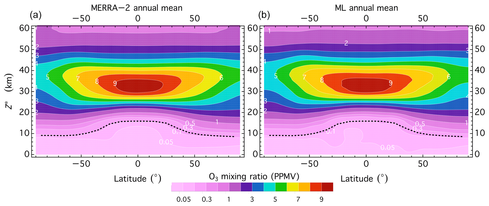
Figure 1 Annual zonal mean O₃ mixing ratio in parts per million by volume as a function of latitude and pressure altitude Z^*. Panel (a) is from the new O₃ profile climatology described in this paper, and panel (b) is from the ML climatology (McPeters and Labow, 2012). The dotted black line in each panel indicates the pressure altitude of the annual zonal mean tropopause. The pressure altitude Z^* is defined as $\mathrm{16}{\log }_{\mathrm{10}}\left[\frac{p_{\mathrm{s}}}{p}\right]$, where p is pressure level (hPa) and p_s=1013.25 hPa.

O₃ profile climatologies (e.g., Wellemeyer et al., 1997; Fortuin and Kelder, 1998; Bhartia and Wellemeyer, 2002; Lamsal et al., 2004; McPeters et al., 2007; McPeters and Labow, 2012; Wei et al., 2010; Bak et al., 2013; Sofieva et al., 2014; Labow et al., 2015) usually provide the a priori profiles for O₃ retrieval from nadir-viewing satellite observations. Most of these climatologies are constructed by merging lower-atmosphere ozonesonde data with upper-atmosphere O₃ profile measurements from one or more satellite instruments, such as the Microwave Limb Sounder (MLS) and the Stratospheric Aerosol and Gas Experiment II (SAGE-II) on the Upper Atmosphere Research Satellite (UARS), the MLS on Aura, or the Solar Backscatter Ultraviolet (SBUV) and SBUV/2 on NASA and NOAA satellites. All these climatologies capture the main characteristic of O₃ vertical distribution, which is determined by the balance of the chemical processes of O₃ production and destruction, as well as by atmospheric motions. Specifically, the vertical O₃ distribution varies strongly with latitude, as shown in Fig. 1. The highest O₃ mixing ratio is found at an altitude of 30–40 km in the equatorial region (see Fig. 1), in which most atmospheric O₃ production induced by strong solar ultraviolet (UV) radiation takes place. The peak values of O₃ profiles in the mixing ratio decrease with higher latitudes, as the large-scale meridional Brewer–Dobson circulation carries the O₃ in the tropical stratosphere towards the poles, and slowly transfers the O₃ to the lower stratosphere at middle and high latitudes. As a result of this atmospheric-circulation-driven process of transport, descent, and accumulation, O₃ profiles in partial pressure or number density exhibit higher maximum values occurring at lower altitudes as latitude increases towards the poles (see Fig. 13). In addition to latitude dependence, some climatologies (e.g., Fortuin and Kelder, 1998; McPeters et al., 2007; McPeters and Labow, 2012; Wei et al., 2010; Bak et al., 2013; Sofieva et al., 2014) include monthly zonal mean O₃ profiles to describe systematic profile changes caused by the seasonal variations in O₃ photochemistry and atmospheric circulation, as well as significant hemispheric profile asymmetry resulting from hemispheric differences in orography, atmospheric temperature, and circulation transport (Maeda and Heath, 1983; Perliski and London, 1989; Cariolle et al., 1992). While the seasonal dependence is accounted for in these O₃ profile climatologies, they have not included the diurnal cycle of O₃, which is significant in the upper stratosphere and mesosphere (Haefele et al., 2008; Huang et al., 2008; Sakazaki et al., 2013; Schranz et al., 2018).

Tropopause marks the interface between the stratosphere and the troposphere, across which there is a steep vertical gradient in O₃ mixing ratio, which is higher in the stratosphere than in the troposphere (see Fig. 1). In the lower stratosphere (between the tropopause and ∼30 km altitude) where O₃ lifetime is quite long (on the order of weeks or longer), the deviation of O₃ vertical distribution from its climatological mean is mainly controlled by atmospheric dynamics. Consequently, O₃ profile and column amount have large daily variations that are associated with meteorological conditions (Reed, 1950). In particular, the rise and fall of tropopause affect O₃ columns and their vertical profiles directly through shifting the O₃ mixing ratio gradient in the upper troposphere and the lower stratosphere (UTLS). This dynamical connection between total O₃ and tropopause pressure (or altitude) has been investigated and documented in a number of studies (e.g., Ohring and Muench, 1960; Salby and Callaghan, 1993; Steinbrecht et al., 1998; Krzyścin et al., 1998; Weiss et al., 2001; Varotsos et al., 2004), which reveal a strong positive (negative) correlation between total O₃ and tropopause pressure (altitude). This correlation implies that tropopause height (or pressure) and total O₃ column amount are excellent indicators for selecting O₃ profile shape in the UTLS region, where O₃ profiles have the highest dynamical variability. To capture dynamical profile variations, O₃ profile climatologies have included tropopause-sensitive zonal mean O₃ profiles (Wei et al., 2010; Bak et al., 2013; Sofieva et al., 2014), as well as column classifications for which zonal mean O₃ profiles are compiled for a range of possible total O₃ columns (Wellemeyer et al., 1997; Bhartia and Wellemeyer, 2002; Lamsal et al., 2004; Labow et al., 2015).

The accuracy of the global O₃ measurements from the series of Total Ozone Mapping Spectrometer (TOMS) is owed in large part to the a priori knowledge of O₃ vertical distribution provided by the total-ozone-column-classified O₃ climatology (Bhartia and Wellemeyer, 2002; McPeters et al., 2007) created for the version 8 (V8) total O₃ algorithm. For mapping between the O₃ column and profile, many recent total O₃ algorithms (e.g., Bhartia and Wellemeyer, 2002; Eskes et al., 2005; Veefkind et al., 2006; Van Roozendael et al., 2006, 2012; Lerot et al., 2010, 2014; Loyola et al., 2011; Wassmann et al., 2015) use the TOMS-V8 climatology, which is a combination of latitude and total O₃-dependent profiles, also known as the standard profiles (Bhartia and Wellemeyer, 2002), and the latitude- and month-dependent Labow–Logan–McPeters (LLM) climatology (McPeters et al., 2007). The standard profiles are 21 annual mean O₃ profiles, covering the possible total O₃ ranges in steps of 50 DU for three latitude zones: 225–325 DU at low latitudes, 225–575 DU at mid-latitudes, and 125–575 DU at high latitudes, and they are used to expand the latitude and month dependent LLM climatology to include the variation with total O₃. While the LLM climatology provides latitude-dependent O₃ profiles that capture the north–south asymmetry, the profile dependence on total O₃ taken from the standard profiles is independent of season and makes no distinction between the Northern Hemisphere and Southern Hemisphere, therefore ignoring the hemispheric asymmetry in O₃ profile deviation from the climatological mean. Furthermore, profile changes associated with total column variations represented by the standard profiles exhibit a large morphology difference between two adjacent latitude zones, as a result of these standard profiles being binned over wide (30^∘) latitude zones. Consequently, total O₃ algorithms relying on TOMS-V8 O₃ profile climatology for profile specification usually have systematic latitudinal biases in retrieved O₃ columns due to the use of hemispherically symmetric and time-independent profile adjustments, and O₃ column discontinuities across the latitude zone boundaries due to large morphology differences. The deficiency of symmetric profile changes may be addressed with the newer column-dependent O₃ climatologies with hemispheric separation (Lamsal et al., 2004; Labow et al., 2015), but their latitude dependencies are compiled on the same 30^∘ wide latitude zones as the standard profiles, with a coarse (semi-annual) seasonal variation (Lamsal et al., 2004) or without seasonal distinction (Labow et al., 2015).

Since the TOMS-V8 climatology is widely used today by many different total O₃ algorithms, there is a need to eliminate its deficiencies by creating a new O₃ profile climatology. The primary objective of the investigation presented in this paper is to develop a new column-classified O₃ climatology using recent data to provide realistic a priori O₃ profile specifications in total O₃ retrievals from the ultraviolet (UV) observations from the Earth Polychromatic Imaging Camera (EPIC) on board the Deep Space Climate Observatory (DSCOVR) satellite, the Ozone Mapping and Profiler Suite Nadir Mapper (OMPS-NM) on the Suomi National Polar Partnership (SNPP) and NOAA-20 satellites, the Ozone Monitoring Instrument (OMI) on Aura, or any other instruments on current and future satellites.

Profile O₃ retrieval algorithms based on the optimal inversion method (Rodgers, 2000) need not only a priori O₃ profiles but also the associated profile covariance matrices to constrain the retrieved profiles. However, O₃ climatologies (e.g., McPeters et al., 2007; McPeters and Labow, 2012; Bak et al., 2013; Sofieva et al., 2014) that are frequently employed in profile retrievals do not contain information about O₃ profile covariance; instead the needed covariance matrices are constructed by assuming positive covariance between different atmospheric layers (e.g., Hoogen et al., 1999; Liu et al., 2005; Bhartia et al., 2013; Miles et al., 2015). This assumption is often unrealistic, as O₃ profile changes resulting from atmospheric vertical motions usually have negative correlations among layers in the UTLS. Improved knowledge about the variability of O₃ vertical distributions, especially how changes among different layers are related, benefit both profile and total column retrievals. Therefore, it is important to develop a new O₃ profile climatology that provides quantitative information about O₃ profile covariance.

3 MERRA-2 O₃ field

The Modern-Era Retrospective Analysis for Research and Applications version 2 (MERRA-2, Bosilovich et al., 2015; Gelaro et al., 2017) reanalysis project produces assimilated data products, including meteorological fields (such as atmospheric temperature and tropopause pressure and altitude) and an O₃ field. This global O₃ field is driven by atmospheric dynamics and constrained by satellite O₃ measurements and is continuous in time and three-dimensional space. Beginning in October 2004, Aura MLS provides constraints on the O₃ profile from the lower mesosphere to the upper troposphere. Though MLS does not have information from the lower troposphere, Aura OMI and MLS jointly provide constraints on the tropospheric O₃ column, with its vertical distribution controlled by atmospheric transport and simplified chemistry with parameterized O₃ loss implemented in the MERRA-2 assimilation system (Wargan et al., 2015; Bosilovich et al., 2015). Evaluation of MERRA-2 O₃ shows excellent agreement between the assimilated O₃ profile in the stratosphere and upper troposphere (between 1 and 500 hPa) with independent satellite and ozonesonde measurements. It also shows that MERRA-2 assimilation realistically reproduces the stratospheric and upper-tropospheric O₃ variability (Wargan et al., 2015, 2017). In the lower troposphere, the correlations between MERRA-2 O₃ profiles and the coincident ozonesonde measurements are lower than the correlations in the UTLS (Wargan et al., 2015, 2017). But the tropospheric O₃ columns (which are O₃ amounts resulting from surface-to-tropopause profile integration) agree very well and have a high degree of correlation with the corresponding columns from ozonesonde measurements (Ziemke et al., 2014), validating the integrated tropospheric profiles of MERRA-2. In short, a MERRA-2 assimilated O₃ field provides a realistic representation of atmospheric O₃ that faithfully captures both short-term (daily or shorter) variations and seasonal changes in vertical and horizontal distributions and thus contains vast information to be harvested for improved characterization of O₃ vertical distributions and variations.

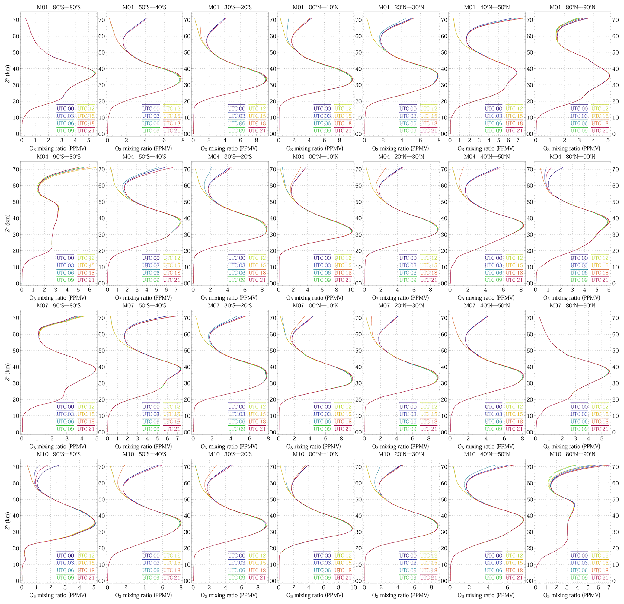
Figure 2 MERRA-2 monthly mean O₃ profiles for four months (January, April, July, and October) and seven tiles that cover the same longitude range (0–15^∘ E) and seven different latitude zones (90–80^∘ S, 50–40^∘ S, 30–20^∘ S, 00–10^∘ N, 20–30^∘ N, 40–50^∘ N, and 80–90^∘ N). Each profile (plotted as a colored line) is calculated from samples with the same UTC time, with different colors representing different UTC times shown in the legend. These mean profiles are averages over 15^∘ longitude, which is equivalent to 1 h of local solar time (LST).

4 MERRA-2 O₃ and temperature profile climatologies

The MERRA-2 record since the Aura MLS and OMI assimilation, owing to its realistic representation of atmospheric O₃, is suitable for creating climatologies to provide improved knowledge of O₃ and temperature vertical distributions.

The long-term MERRA-2 record is stored as a four-dimensional (latitude, longitude, atmospheric pressure, and time) data set that covers the globe uniformly at high spatial and temporal resolutions. More precisely, the global coverage is provided at 3-hourly intervals with a horizontal resolution of 0.5^∘ latitude by 0.625^∘ longitude and a vertical grid covering 72 layers between the surface and 0.01 hPa. The MERRA-2 O₃ profiles from 2005 to 2016, within the period of Aura MLS and OMI assimilation, are analyzed to create a new O₃ profile climatology. The enormous number of data from this period facilitate reliable statistical representation of mean O₃ profiles and their variations on more finely resolved dependent variables, including tropopause pressure, total column amount, latitude, longitude, and time.

MERRA-2 data fields (such as O₃ and temperature profiles) are represented on a hybrid terrain-following pressure coordinate (Wargan et al., 2017), and thus have the lowest altitude level at the surface. These data fields are interpolated or extrapolated (for grids below the surface down to the sea level) to the uniform pressure altitude grid before statistical computation to create sea-level-based MERRA-2 climatologies. Here the pressure altitude, $Z^{*}=\mathrm{16}{\log }_{\mathrm{10}}\left[\frac{p_{\mathrm{s}}}{p}\right]$, is a dimensionless quantity, but is assigned units of kilometers because it is quite close to the altitude (km) at pressure level p above the surface at p_s=1013.25 hPa, with a difference usually less than 1 km when Z^*≲30 km.

4.1 Local-solar-time-dependent O₃ profile climatology

The photochemical O₃ production and destruction depend strongly on solar illumination, which changes systematically for a location during the course of a day, resulting in diurnal variation in O₃ vertical profiles (Haefele et al., 2008; Huang et al., 2008; Sakazaki et al., 2013; Schranz et al., 2018), but existing O₃ profile climatologies have not included O₃ profile dependence on local solar time. Remote sensing O₃ measurements are collected at different local solar times, even from the same instrument, such as the DSCOVR EPIC, which observes the Earth from sunrise to sunset simultaneously (Herman et al., 2017). Proper accounting for the diurnal variations in O₃ vertical distribution would enable more accurate O₃ retrieval from remote sensing observations. Therefore we construct a local-solar-time-dependent O₃ profile climatology from the MERRA-2 O₃ field.

We divide the globe equally into 24×18 rectangle tiles, and each has the size of 15^∘ longitude × 10^∘ latitude. Monthly mean profiles and their variances are calculated from samples that fall within a tile at the eight UTC times of the MERRA-2 O₃ field. Note that data samples are weighted by the cosine of latitude in performing the statistics to ensure equal weighting by area. Since each climatological profile of a tile is compiled from O₃ profiles at the same UTC, it represents an hourly mean because a tile's 15^∘ longitude range is equivalent to 1 h of local solar time (LST).

Figure 2 shows the sample O₃ profiles from the MERRA-2 local-solar-time-dependent climatology, illustrating the diurnal, seasonal, and latitudinal variations in O₃ vertical distributions. Each panel in Fig. 2 contains plots of eight climatological O₃ mixing ratio profiles for a tile next to and east of the prime meridian, for eight different 1 h LST periods. The differences among the curves in a panel reveal the diurnal O₃ mixing ratio changes, which in general increase significantly with altitude from the upper (Z^*≳30 km) stratosphere into the mesosphere (Z^*≳50 km). The O₃ mixing ratio level in the mesosphere reaches its minimum after sunrise but then increases after sunset, recovering its nighttime value quickly, while in the stratosphere where the peak value of O₃ mixing ratio is located (Z^* between ∼35 and 40 km), O₃ diurnal cycle has its maximum in the afternoon and a lower value close to its minimum in the morning. The diurnal variations, which are mainly driven by photochemistry in the upper atmosphere, exhibit a strong latitudinal (panel rows in Fig. 2) and seasonal (panel columns) dependence, as expected from the variations in solar insolation with the latitude and the season. The mean nighttime O₃ mixing ratio can be an order of magnitude higher than the daytime value in the mesosphere at $Z^{*}=\mathrm{70}$ km. In general, the magnitude of diurnal difference reduces with the altitude, with a maximum of ∼7 % near the stratospheric O₃ mixing ratio peak. In the troposphere, the cycle of diurnal variation changes with season and location, with a peak-to-trough difference usually less than 5 % in the lower troposphere. These significant diurnal O₃ mixing ratio variations correspond to typically 0.5 % and a maximum of ∼4 % peak-to-trough differences in diurnal variation in total O₃ vertical column. The variability of the tropospheric O₃ profile, including the diurnal cycle, is mostly subdued in the MERRA-2 O₃ field because the assimilation captures only the average behavior of tropospheric O₃ but not its variation realistically, a consequence of the limited tropospheric O₃ information contained in the source data (OMI columns and MLS profiles). The results for the mesosphere and stratosphere are in general consistent with previous findings of O₃ diurnal variations (Haefele et al., 2008; Huang et al., 2008; Sakazaki et al., 2013; Schranz et al., 2018, and references therein). Thus, this local-solar-time-dependent climatology correctly captures diurnal variation in upper-atmospheric O₃ vertical distributions.

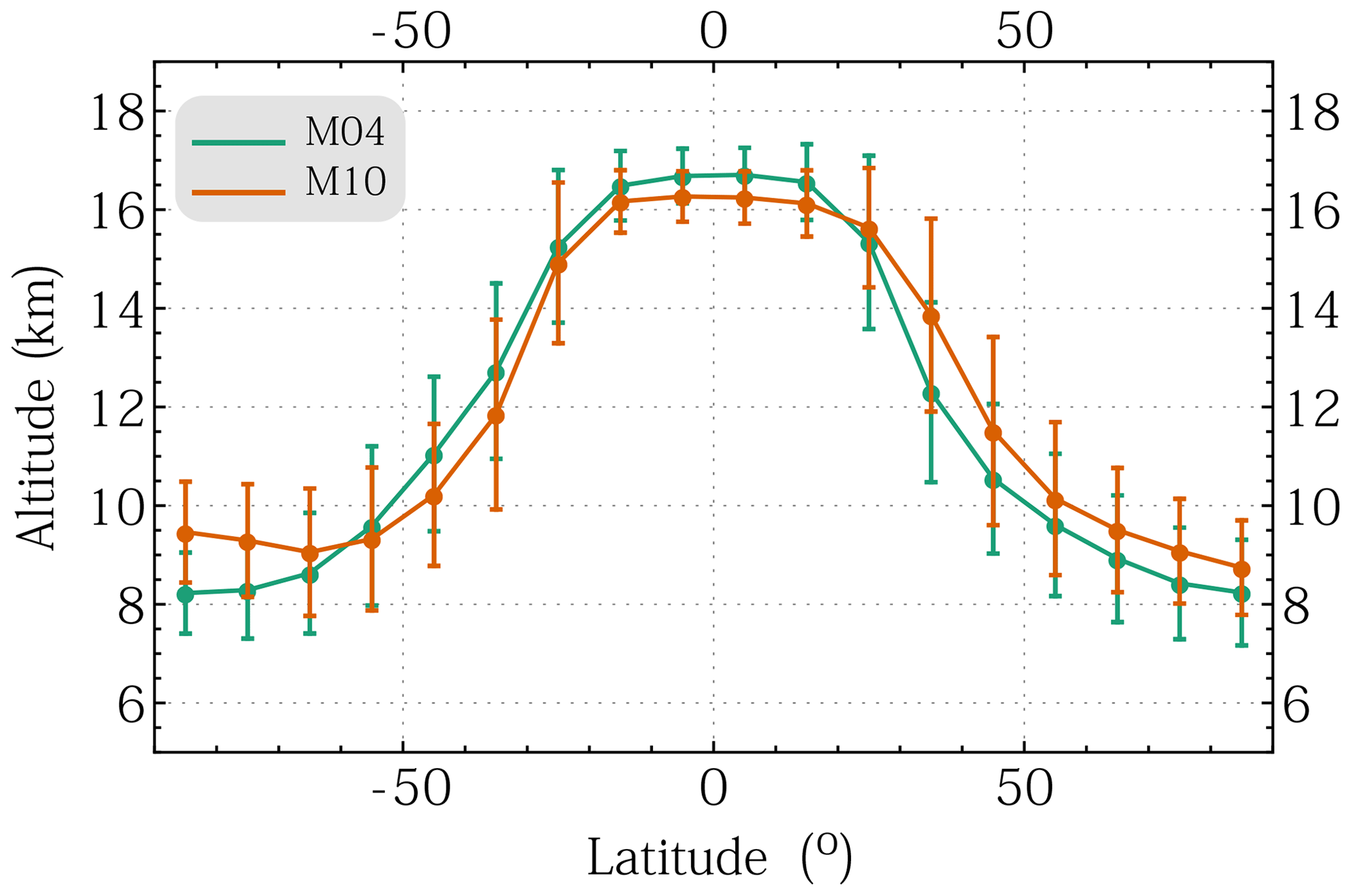
Figure 3 MERRA-2 daytime monthly zonal mean tropopause altitude and its standard deviation as a function of latitude for April (M04) and October (M10).

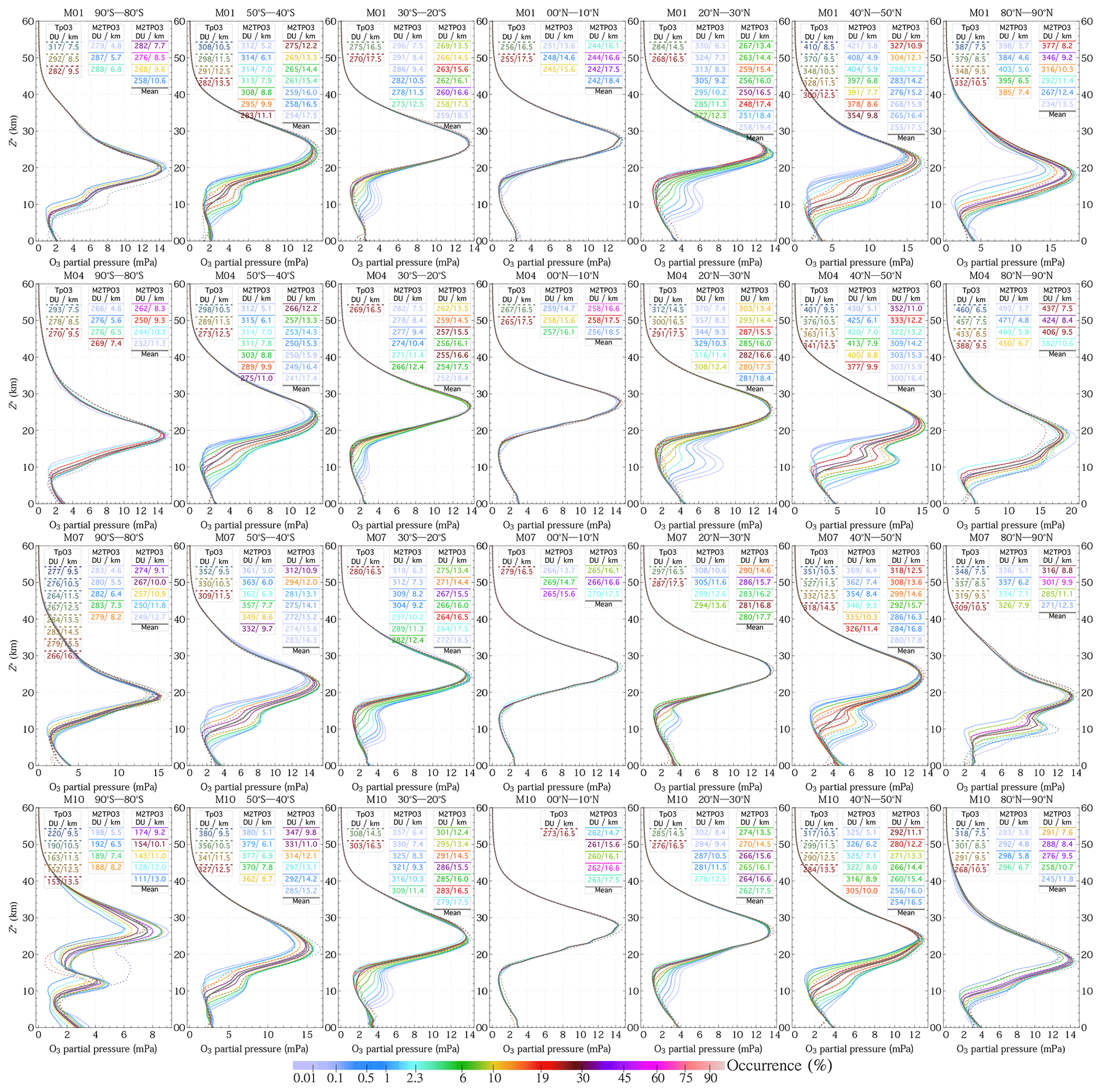
Figure 4 Profile comparisons between M2TPO3 and TPO3 of Sofieva et al. (2014) for four months (January, April, July, and October) and seven latitude zones (90–80^∘ S, 50–40^∘ S, 30–20^∘ S, 00–10^∘ N, 20–30^∘ N, 40–50^∘ N, and 80–90^∘ N). Colored solid lines represent M2TPO3 profiles, while the dotted ones represent TPO3 profiles. The color of a solid line indicates the percentage occurrence of the profile, which is calculated as the percentage of profiles in the month–latitude class that fall within the Z^* tropopause pressure bin. The line legends display the average tropopause altitude and the average total O₃ column for the corresponding climatological profile. The solid gray line represents the downgraded M2TPO3 profile, i.e., the monthly zonal mean profile.

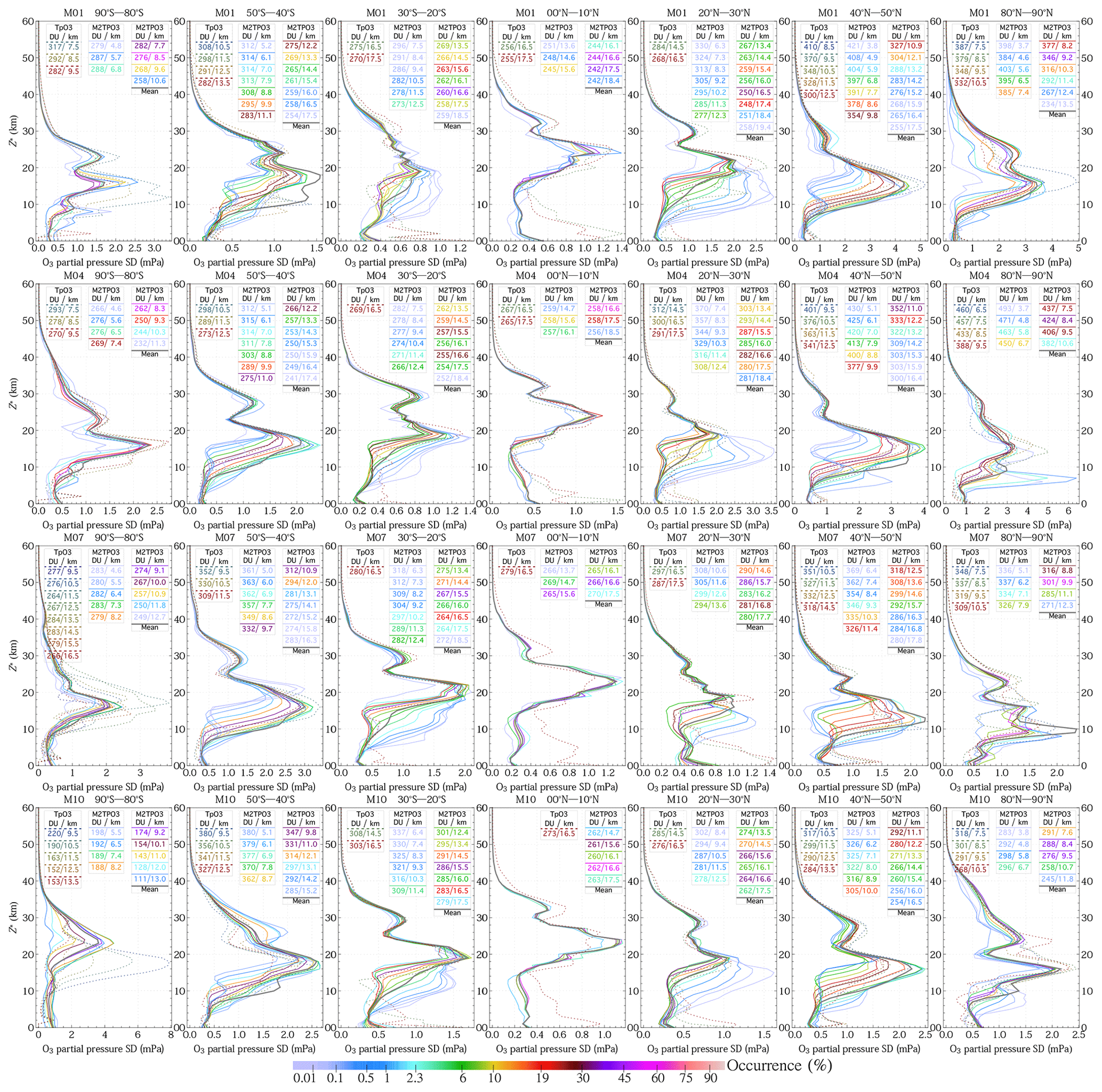
Figure 5 Similar to Fig. 4, but for standard deviation (SD) comparisons between M2TPO3 and TPO3 of Sofieva et al. (2014).

4.2 Tropopause-pressure-classified O₃ profile (M2TPO3) climatology

Tropopause altitude varies with month and latitude systematically (Hoinka, 1998) and is usually highest in the tropics and drops toward the poles with steep declines in the midlatitudes but exhibits hemispheric asymmetry (e.g., see Fig. 3). This figure also illustrates that the dynamic variability of tropopause altitude is characterized by daily standard deviations of approximately 1–2 km, which agrees well with the characterization by Seidel and Randel (2006). Since O₃ concentration is highest in the lower stratosphere above the tropopause and decreases rapidly in the troposphere, the large short-term fluctuation of tropopause altitude results in high variability in the total O₃ column, accounting for ∼60 % of its daily variation (Wei et al., 2010). Thus grouping O₃ profiles according to the tropopause pressure or altitude generates climatological profiles that reflect the dynamical influences on O₃ vertical distributions, as demonstrated by the tropopause-altitude-classified O₃ profile climatology (named the TPO3 climatology) created by Sofieva et al. (2014) using ozonesonde and SAGE-II data.

Similarly, we create a tropopause-pressure-classified O₃ profile climatology (referred to as M2TPO3 climatology hereafter) using the MERRA-2 O₃ record, which provides a large number of data covering a diverse range of conditions, likely including all possible tropopause pressures. These mean profiles and their variances are calculated by statistically analyzing the sets of MERRA-2 O₃ profiles at the same UTC time, binned by tropopause pressure in 1 km pressure altitude (Z^*) steps, calendar month, and 15^∘ × 10^∘ longitude–latitude tiles. To compare the M2TPO3 with the TPO3 (Sofieva et al., 2014), we create a daytime zonal mean climatology by combining M2TPO3 tiles with the same latitude zone and LST from 09:00 through 17:00. The resulting daytime climatology contains 2154 mean profiles and standard deviations (shown in Appendix A), spanning the range of tropopause pressure (altitude) from 605 hPa (3.56 km) to 62 hPa (19.3 km), distributed in 12 calendar months and 18 10^∘ latitude zones that cover the latitude range from −90 to 90^∘.

Figures 4 and 5 display a subset of daytime M2TPO3 profiles and standard deviations and their comparisons with those of TPO3 (Sofieva et al., 2014). The results in Fig. 4 show that both M2TPO3 and TPO3 have similar O₃ profile shapes for similar tropopause altitudes in each month–latitude class. Especially in the tropics, M2TPO3 and TPO3 show very close profiles that are nearly independent of tropopause altitude and season. For profiles at higher latitudes, Fig. 4 illustrates that the profile change associated with tropopause altitude variation occurs mostly below the O₃ concentration peak, exhibiting increasing UTLS O₃ with lower tropopause altitude. The O₃ column amounts (displayed in the figure legends) of TPO3 profiles are generally (about 1 % to 4 %) higher than the corresponding M2TPO3 profiles. This comparison indicates that there is likely a slight positive bias in the total columns in the TPO3 climatology since MERRA-2 total O₃ columns have a latitude-dependent (up to 2 %) low biases (Wargan et al., 2017). Comparing with the TPO3, there are more tropopause pressure bins with sufficient samples for reliable statistics, and hence more M2TPO3 profiles corresponding to a broader range of tropopause altitudes in each month–latitude class. Under the O₃ hole condition, strong O₃ spatial variations sampled differently by ozonesondes likely contribute to significant profile differences between M2TPO3 and TPO3 (see Fig. 4 lower left panel). Note that TpO3 is binned in 1 km tropopause altitude steps, and the corresponding legend shows the midpoint of the altitude bin. Consequently, the tropopause altitude in the legends of Fig. 5 changes regularly (in 1 km steps). On the other hand, M2TOP3 is binned in 1 km Z^* tropopause pressure altitude steps, and the average tropopause altitude of the binned profiles is displayed in the corresponding legend. This average value does not change regularly from one bin to the next because the distribution of tropopause altitude is not necessarily symmetric with respect to the bin center.

The standard deviations in Fig. 5 show similar magnitudes and vertical structures between the M2TPO3 and the TPO3 profiles with similar tropopause altitudes, demonstrating that the M2TPO3 climatology represents O₃ variability realistically. The main differences occur in the lower troposphere of tropical latitude zones, where TPO3 shows higher variability than the M2TPO3, due to ozonesondes better capturing the influence from tropospheric O₃ productions, which are not explicitly included in the MERRA-2 reanalysis. Significant differences are also observed over polar latitude zones (90–80^∘ S and 80^∘ N–90^∘ S), likely due to differences in sampling over highly inhomogeneous spatial distributions in these zones.

Results in Fig. 5 show that the standard deviations of the high-occurrence profiles are in general smaller than those for the downgraded (monthly zonal mean) profile, indicating that tropopause pressure is a good predictor of O₃ profile shape, leading to a more accurate profile specification than simply taking the monthly zonal mean profile.

The comparison in this section shows overall good agreement of the M2TPO3 means and standard deviations versus those of the TPO3, with an expected discrepancy in the O₃ variability in the tropical lower troposphere, validating the realism of MERRA-2 O₃ record and its suitability for climatology construction.

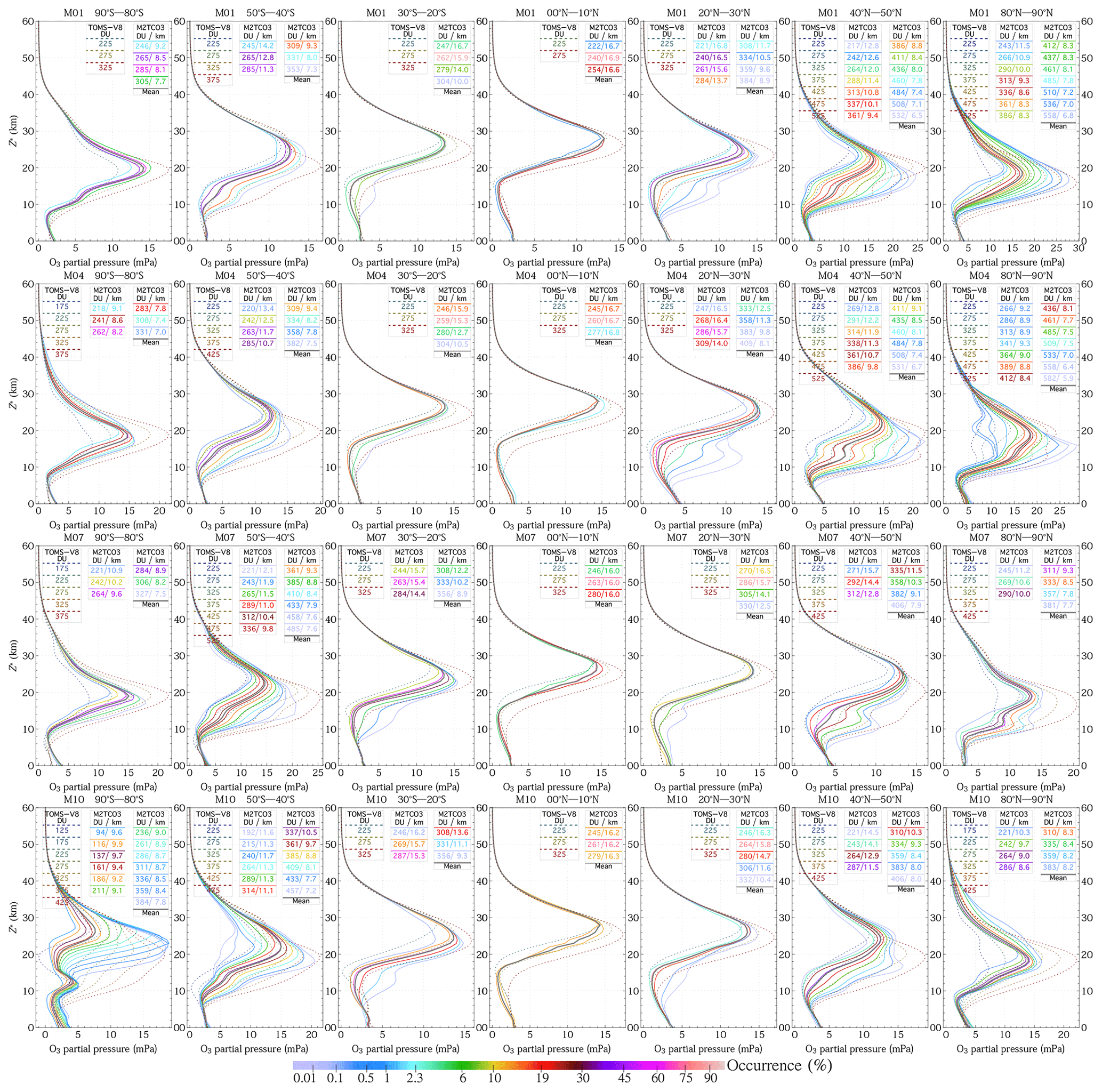
Figure 6 Profile comparisons between M2TCO3 and TOMS-V8 for four months and seven latitude zones (same as those in Fig. 4). Colored solid lines represent M2TCO3 profiles, while the dotted ones represent TOMS-V8 profiles. The color of a solid line indicates the percentage occurrence of the climatological profile, and its line legend displays the average tropopause altitude and the average total column O₃. The solid gray line represents the downgraded M2TCO3 (monthly zonal mean) profile, which is the same as the downgraded M2TPO3 profile shown in Fig. 4. Note that since the total O₃ distribution is usually not symmetric with the bin center, the average total O₃ column does not change regularly from one bin to the next (see O₃ columns in the legends). On the other hand, TOMS-V8 profiles are created to cover preset (latitude-zone-dependent) O₃ column ranges in 50 DU steps.

Figure 7 Standard deviation (SD) comparisons between M2TPO3 and M2TCO3 for four months and seven latitude zones (same as those in Fig. 4). Colored solid lines represent M2TCO3 SDs, while colored dotted lines represent M2TPO3 SDs. The color of a solid or dotted line indicates the percentage occurrence of the climatological profile, and its line legend displays the average tropopause altitude and the average total column O₃. Only SDs for climatological profiles with greater than 5 % occurrence are plotted. The solid gray line represents the downgraded M2TCO3 profile SD, i.e., the SD for the monthly zonal mean profile, and it is identical to the SD of the downgraded M2TPO3 profile. The SDs quantify the natural variability of O₃, and a smaller one signifies that the climatological mean provides a more reliable O₃ profile specification.

4.3 Total-column-classified O₃ profile (M2TCO3) climatology

The tropopause-pressure-dependent O₃ profiles contained in the M2TPO3 climatology capture profile changes resulting from short-term meteorological disturbances in the UTLS region. The near-linear relationship between mean total column O₃ and tropopause altitude (e.g., see legend tables in Fig. 4) quantified for each month–latitude class implies that the total column O₃ may serve as a good predictor of O₃ profile shape as well. Grouping profiles by total column O₃ may actually better capture O₃ distribution and variability driven by both dynamical and chemical processes; we therefore create a total-column-classified O₃ profile climatology (referred to as the M2TCO3 climatology hereafter) from the long-term MERRA-2 O₃ record.

The M2TCO3 climatology is constructed by binning the MERRA-2 O₃ field at the same UTC time by total column in 25 DU steps, calendar month, and 15^∘ × 10^∘ longitude–latitude tiles. To compare the M2TCO3 with the TOMS-V8 (Bhartia and Wellemeyer, 2002; McPeters et al., 2007), we create a daytime zonal mean climatology by combining M2TCO3 tiles with the same latitude zone and LST from 00:09 through 17:00. The resulting climatology contains 1644 mean profiles and standard deviations (shown in Appendix A), spanning the range of total O₃ from 94 to 584 DU, distributed in 12 calendar months and 18 latitude zones that cover the latitude range from −90 to 90^∘. Figure 6 displays a subset of daytime M2TCO3 profiles and the corresponding TOMS-V8 profiles, illustrating the distinct characteristics of O₃ vertical distributions, as well as significant differences between the two climatologies. Both M2TCO3 and TOMS-V8 profiles exhibit higher altitudes of O₃ peak with lower O₃ columns for a month–latitude class, lower peak altitudes with higher latitudes for a total O₃ column, narrow dynamical O₃ ranges and nearly identical profile shapes for different seasons in the tropics but higher seasonal and dynamical variations in midlatitude and high-latitude regions, and hemispherical asymmetry.

The differences between M2TCO3 and TOMS-V8 (shown in each panel of Fig. 6) reflect the improvements in the realism of O₃ profile representation with the M2TCO3 climatology. The column-averaged TOMS-V8 profiles are represented by the LLM climatology (McPeters et al., 2007), which is updated to the (McPeters and Labow, 2012) (ML) climatology, and are very close to the downgraded M2TCO3 profiles (see comparisons in Figs. 1 and 13). Therefore the differences between M2TCO3 and TOMS-V8 profiles shown in Fig. 6 are attributed to the profiles deviations applied to the mean derived from the standard column-dependent profiles of TOMS-V8 (Bhartia and Wellemeyer, 2002), which are independent of season, coarse in latitude resolution, and symmetric with respect to the Equator. These deficiencies limit the realism of TOMS-V8 climatological profiles, and are eliminated with the new M2TCO3 climatology, which provides improved O₃ profile representation that better captures profile changes associated with column variations and their dependence on season and latitude.

The total O₃ range of the TOMS-V8 climatology is the same as the set of TOMS-V8 standard (annual mean) profiles. These preset (latitude-zone-dependent) ranges may be different (narrower or broader) than those of M2TCO3 at some months and latitude zones (see Fig. 6), but they are likely inconsistent with actual O₃ range due to the imposition of annual O₃ range on the monthly variation.

Figure 7 shows the standard deviations of a subset of M2TCO3 profiles with high (>5 %) occurrence percentage and comparisons with those of M2TPO3. A vast majority of high-occurrence climatological profiles of M2TCO3 and M2TPO3 shown in Fig. 7 exhibit significantly reduced standard deviations compared to those of monthly zonal mean (i.e., downgraded) profiles, illustrating that both tropopause pressure and total column O₃ provide information for more precise specification of O₃ profiles. Comparisons between M2TPO3 and M2TCO3 show that column classification usually leads to greater reductions in standard deviations in the upper stratosphere but smaller ones in the UTLS than tropopause pressure classification. Since there is much more O₃ in the upper stratosphere than below, an overall more realistic specification of the O₃ profile is achieved using the M2TCO3 climatology based on the total column O₃ than using the M2TPO3 based on the tropopause pressure. Hence the column-dependent climatology is most appropriate in mapping between the O₃ column and vertical profile needed in total O₃ column retrieval algorithms. However, with the knowledge of tropopause pressure, the tropopause-dependent climatology usually provides closer matches to actual profiles and stronger constraints in the UTLS; therefore its usage significantly improves the accuracy of O₃ profile retrieval (Bak et al., 2013) from backscattered UV measurements, which have lower vertical resolutions in the troposphere than in the stratosphere (Liu et al., 2010).

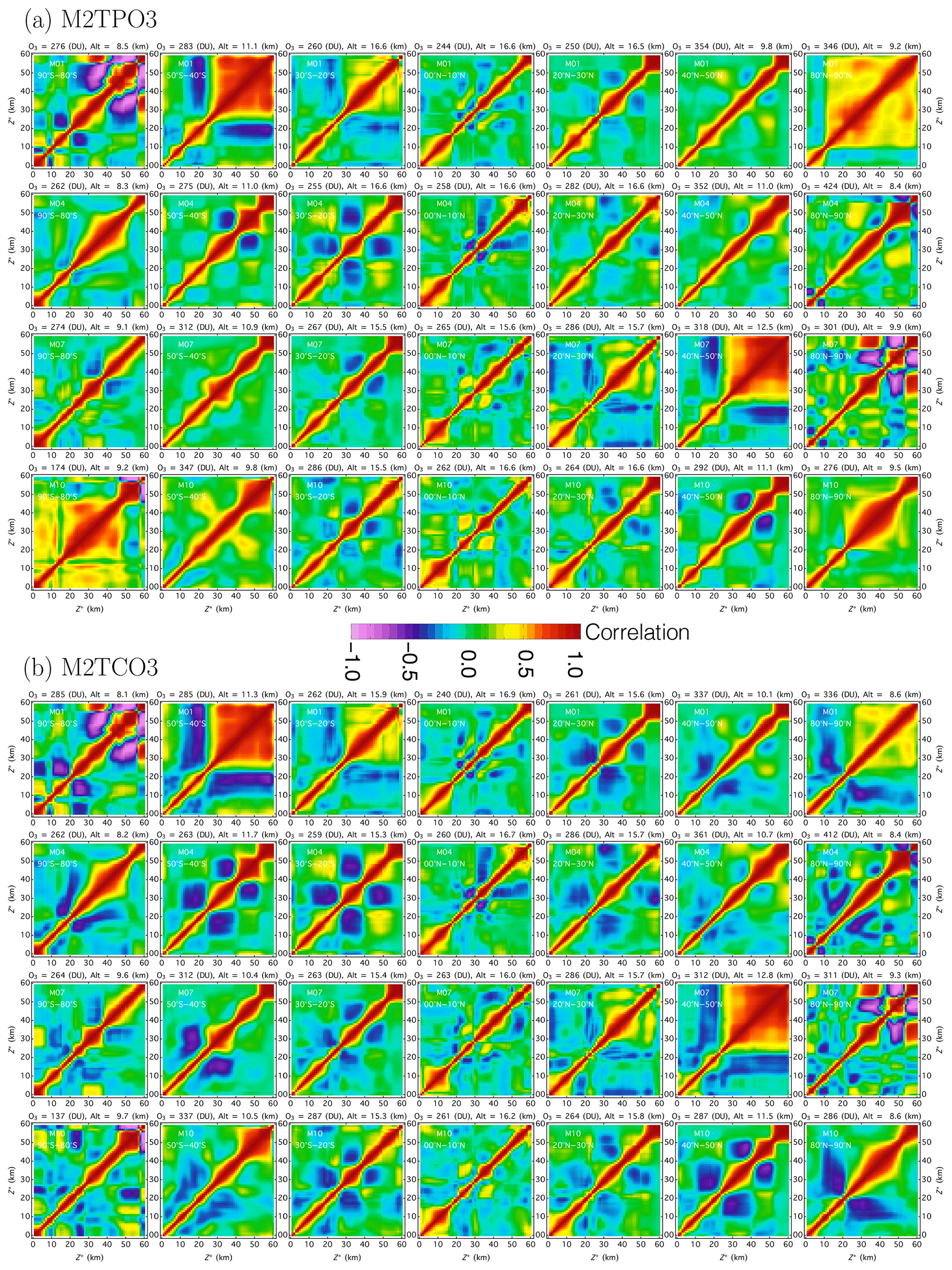
Figure 8 Correlation matrices from M2TPO3 (a) and M2TCO3 (b) for four months and seven latitude zones (same as those in Fig. 4). Here the matrix for the highest-occurrence climatological profile is shown for each month–latitude class.

Figure 9  

4.4 O₃ profile covariance climatology

Previous O₃ climatologies (e.g., Fortuin and Kelder, 1998; McPeters et al., 2007; McPeters and Labow, 2012; Bak et al., 2013; Sofieva et al., 2014) used in O₃ profile retrievals include profile standard deviations but not information about O₃ profile covariance because their sources (ozonesonde and satellite measurements) have limited coincident samples to quantify the joint O₃ variability between different altitudes throughout the atmosphere. In contrast, the MERRA-2 assimilation provides complete profiles simultaneously, allowing direct statistical computation of profile covariance matrices. We expand the classification analysis to quantify the O₃ profile covariance. Specifically, we construct an O₃ profile covariance matrix from each bin used for the calculation of an M2TPO3 or M2TCO3 climatological profile. The resulting covariance climatology first provides quantification of O₃ vertical distribution variabilities, the correlations among different levels, and their dependence on tropopause pressure or total column O₃ for different months and longitude–latitude tiles.

Figure 8 shows a subset of correlation matrices, which are standardized, i.e, diagonal element normalized to covariance matrices, from the daytime M2TPO3 and daytime M2TCO3 climatologies. These density plots highlight the varying degree of level-to-level correlations and their contrasts with the diagonal-constant matrices typically used in O₃ profile retrievals (e.g., Hoogen et al., 1999; Liu et al., 2005; Miles et al., 2015), which assume positive layer-to-layer correlation that decreases monotonically and exponentially with distance between layers. Contrary to this typical assumption, Fig. 8 illustrates that the degree of correlation between two levels fluctuates with the level separation and negative correlations are quite common.

The quantification of O₃ profile covariance offers a new way to represent O₃ vertical distribution realistically and efficiently. Figure  shows the first three leading empirical orthogonal functions (EOFs), which are the ordered set of eigenvectors for each covariance matrix shown in Fig. 8. Typically the first three leading EOFs combined explain between 65 % and 85 % of the class variance, and the first 15 leading EOFs account for over 95 % of the class variance. Much like a climatological profile describes the likely O₃ vertical distribution, the EOFs describe the most probable patterns of profile deviations from the climatological mean. In general, an O₃ profile X can be expressed as

$$\begin{array}{}\text{(1)}& \mathbf{X}={\mathbf{X}}_{\mathrm{m}}+\sum _{k=\mathrm{1}}^{\mathrm{n}}{\mathit{\omega }}_k{\mathbf{e}}_k,\end{array}$$

where X_m is a climatological mean profile, e_k the kth EOF, ω_k the kth coefficient, and n the total number of EOFs with its maximum limited to the number of levels used to represent the O₃ profile. Since a high fraction of class variance may be explained with just a few leading EOFs, they provide the most efficient adjustments to improve the representation of O₃ profile when it deviates from the climatological mean. When interpreted physically, the leading EOFs correspond to processes of O₃ accumulation, reduction, or redistribution. For instance, the first three EOFs for an M2TPO3 covariance matrix (see Fig. a) describe (1) column increase or decrease, represented by the EOF-1 (monopole) pattern, (2) up or down shift of a profile, represented by the EOF-2 (dipole) pattern, showing O₃ increase at one altitude and decrease at another, and (3) shrink or stretch of a profile, represented by the EOF-3 (tripole) pattern, showing O₃ decrease (increase) at one altitude and increase (decrease) at adjacent (above and below) altitudes. The results in Fig. a indicate that the highest or the second highest contribution to the variance of a tropopause class originates from the total column variation. However, the highest contribution to the variance of a total column class comes from O₃ profile shift, represented by EOF-1 (dipole) in Fig. b, usually linked with tropopause variation, since the dominant profile change resulting from column variation is accounted for with different O₃ column classes. The second EOF (tripole) of an M2TCO3 covariance matrix describes the shrink or stretch of a profile, similar to the third EOF of an M2TPO3 matrix, while subsequent EOFs describe more complex rearrangement of the O₃ profile.

Figure 10 Climatological temperature profiles corresponding to the M2TCO3 O₃ profiles shown in Fig. 6. The color of a solid line indicates the percentage occurrence of the climatological profile, and its line legend displays the average tropopause altitude and the average total column O₃. The solid gray line represents the monthly zonal mean temperature profile, and the dashed dark blue line shows the coefficient of correlation between O₃ partial pressure and temperature as a function of pressure altitude Z^*.

4.5 Temperature profile climatology

Using the same binning schemes employed in the O₃ profile climatologies, we create temperature profile climatologies from the MERRA-2 assimilated atmospheric temperature field. The resulting climatologies contain the mean and covariance of temperature profiles, paired with the respective M2TPO3 and M2TCO3 climatological O₃ profiles.

Figure  shows sample MERRA-2 climatological temperature profiles corresponding to the sample M2TCO3 climatological O₃ profiles shown in Fig. 6, and the O₃–temperature correlation profiles for the sample month–latitude classes. These results illustrate the systematic behavior among O₃ column amount, tropopause altitude, and atmospheric temperature: higher O₃ column amounts occur with a warmer lower stratosphere and a colder troposphere, the condition for lower tropopause altitudes. This relationship, as well as its dependence on season and latitude, is captured in the MERRA-2 O₃ and temperature climatologies and is consistent with the findings of long-term O₃ and temperature profile measurements (Steinbrecht et al., 1998).

Results in Fig.  also reveal a significant north–south asymmetry in climatological temperature profiles. For instance, the stratospheric temperatures in the austral spring (e.g., see the October panel) in the southern polar region (90–80^∘ S) are significantly lower than those in the boreal spring (e.g., see the April panel) in the northern polar region (80–90^∘ N), and these temperature differences are associated with lower total O₃ columns in the Antarctic than those in the Arctic.

The profile of correlation coefficient in each panel of Fig.  illustrates a mutual relationship between O₃ concentration and atmospheric temperature. From the upper (Z^*≳35 km) stratosphere to the lower mesosphere (Z^*≲60 km), O₃ and temperature are mainly negatively correlated because in this region O₃ concentration is mostly governed by photochemical reactions, for which higher temperature speeds up the rate of O₃ destruction. From the lower stratosphere down to the upper troposphere (10 km ≲Z^*≲ 35 km) in which O₃ concentration is controlled primarily by atmospheric motions (Brasseur and Solomon, 2005), O₃ and temperature are positively correlated since higher O₃ concentrations likely occur from adiabatic air parcel compression, which increases the parcel temperature as well, and additionally higher O₃ concentrations absorb more UV radiation, thus raising the atmospheric temperature. The positive correlation quickly becomes negative as the altitude descends into the lower troposphere (Z^*≲ 10 km), but swings back and may become positive as the altitude falls further. In general, the degree of O₃–temperature correlation is smaller in the lower troposphere than in the atmosphere above, indicating a weaker connection between them.

The pattern of negative correlation above the upper stratosphere and the positive correlation in the upper troposphere and lower stratosphere between O₃ and temperature fields were elucidated with dynamical chemical models (Rood and Douglass, 1985; Froidevaux et al., 1989; Smith, 1995). The O₃–temperature correlation profiles in Fig.  are consistent with those from numerical modeling (Rood and Douglass, 1985) and observational data analysis (Fortuin and Kelder, 1996), indicating that the MERRA-2 O₃ and temperature climatologies represent O₃ and temperature distributions and their interrelationship realistically.

4.6 Spatial distribution of O₃

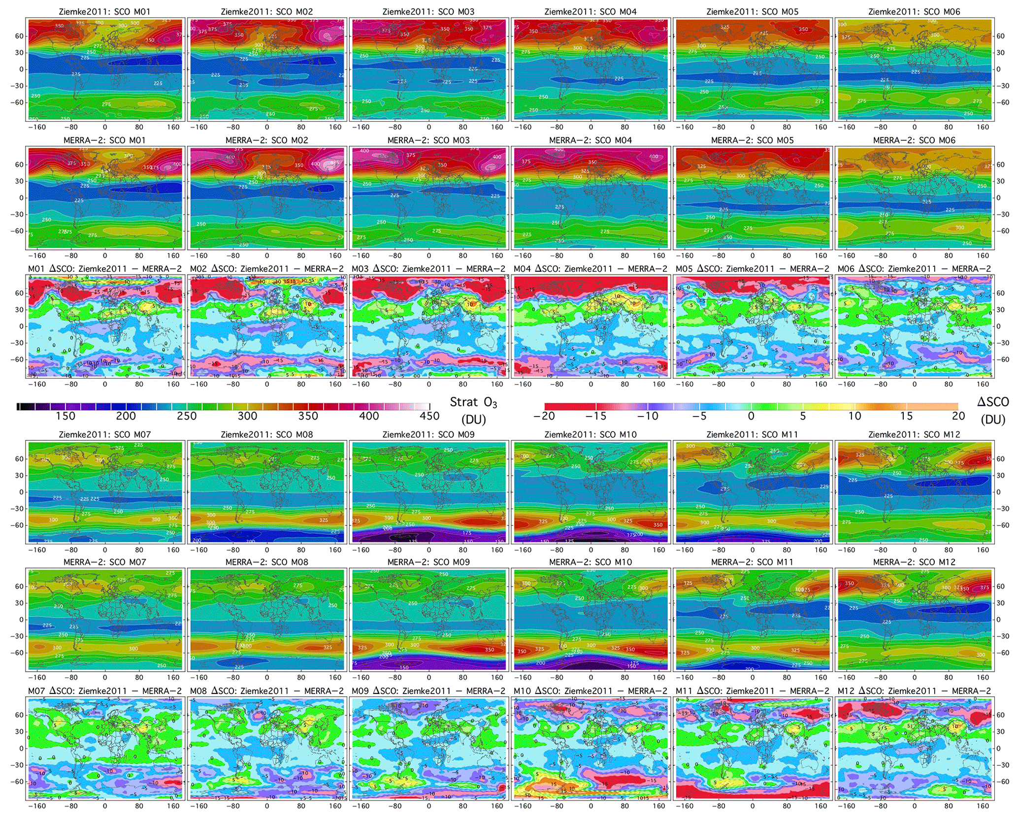
Figure 11 Climatological stratospheric column O₃ (SCO) maps from MERRA-2 and Ziemke et al. (2011) for the 12 months (January–June, upper panels; July–December, lower panels) of the year and their differences.

Figure 12 Similar to Fig. 10, except for tropospheric column O₃ (TCO).

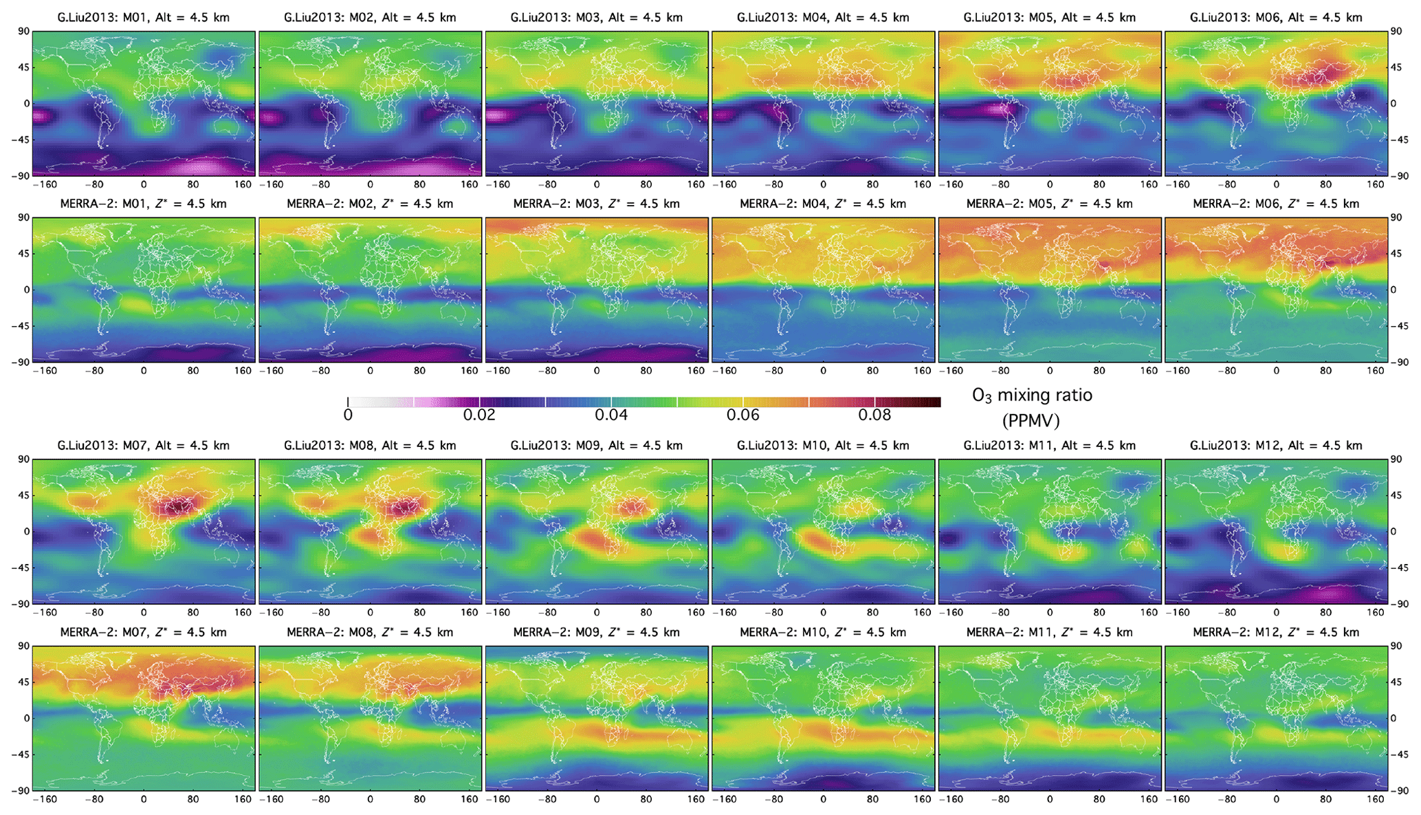
Figure 13 MERRA-2 climatological O₃ concentration (i.e., mixing ratio in parts per million by volume) at $Z^{*}=\mathrm{4.5}$ km for the 12 months (January–June, upper panels; July–December, lower panels) of the year and comparison with the tropospheric O₃ profile climatology of G. Liu et al. (2013). Note that the mixing ratio of G. Liu et al. (2013) is at 4.5 km altitude.

The spatial distribution of O₃ is controlled by the various chemical and dynamical processes that drive the production, destruction, and transport of atmospheric O₃. Since the distributions of O₃ sources and surface topography are inhomogeneous over the globe, systematic patterns with significant longitudinal variations are present in horizontal O₃ distribution. The MERRA-2 baseline climatologies presented in previous sections focus on the latitudinal and altitudinal distribution of O₃, with a coarse longitudinal resolution retained through the binning of the globe with equal size (15^∘ longitude × 10^∘ latitude) tiles. To better capture the spatial variation in O₃ and to compare directly with previous global O₃ climatologies (Ziemke et al., 2011; Liu et al., 2013, referred to respectively as Ziemke2011 and GLiu2013 hereafter), we create a higher-spatial-resolution O₃ profile climatology from MERRA-2 by reducing the tile bin size to 5^∘ longitude × 5^∘ latitude, which is the bin size for both Ziemke2011 and GLiu2013 climatologies. This higher-spatial-resolution MERRA-2 climatology consists of monthly statistics of O₃ volume mixing ratio profile, tropopause pressure, stratospheric column O₃ (SCO), and tropospheric column O₃ (TCO) for 2592 ($=\mathrm{36}\times \mathrm{72}$) 5^∘ × 5^∘ tiles. Here the SCO is an integration of an O₃ profile from 0.01 hPa down to the tropopause and the TCO from the tropopause down to the surface.

For better comparisons with the Ziemke2011 climatology, we partition the MERRA-2 total O₃ column into SCO and TCO using the climatological tropopause pressure provided in Ziemke2011, which is compiled from the National Centers for Environmental Prediction (NCEP) tropopause pressures. Figures 10 and 11 show the spatial distributions of the NCEP-based MERRA-2 SCO and TCO, respectively, for 12 months of the year and their comparisons with Ziemke2011. Results in Figs. 10 and 11 reveal excellent agreement between MERRA-2 and Ziemke2011 in the low-latitude zone (within ±30^∘), with ΔSCO ≲±5 DU and ΔTCO ≲±6 DU for most months and tiles. This agreement becomes worse in the higher-latitude regions, mostly showing larger differences in SCO and TCO between MERRA-2 and Ziemke2011, likely due to higher longitudinal variability in stratospheric O₃, degrading the accuracy of SCO from gap-filling interpolation of Aura MLS data (Ziemke et al., 2011). From September to May, MERRA-2 SCO in the polar latitudes is higher, while TOC is lower than the corresponding columns from Ziemke2011, with the broadest spread occurring in February–April. But more significantly, Figs. 10 and 11 show that both spatial distributions of MERRA-2 SCO and TCO and their seasonal cycles closely resemble those of Ziemke2011.

MERRA-2 SCO displays a strong latitude dependence (see Fig. 10) that is shaped primarily by the Brewer–Dobson circulation, showing low values in the tropics (∼220 DU) and elevated values in the middle and high latitudes, with the highest column amount exceeding 400 DU in the Northern Hemisphere (NH) (between 70 and 80^∘ N) during February–April and exceeding 350 DU in the Southern Hemisphere (SH) (between 45 and 60^∘ S) in September–October. The SCO longitudinal variability is low in the tropics but increases significantly along with higher columns at midlatitudes and high latitudes. In the midlatitude to high-latitude regions centered around 60^∘ N, the longitudinal variation exhibits an oscillatory pattern with high SCO over North America that stretches across the Pacific Ocean to over eastern Asia. This pattern, which is influenced by the semipermanent atmospheric pressure systems resulting from the unique orography distribution in the NH, persists over the year with amplitude varying with the season and reaching its maximum during February. In the SH, a wavelike high-SCO pattern with longitude center near the dateline (the 180th meridian) also appears in the middle–high-latitude band (around 60^∘ S), which evolves with the progression of the Antarctic O₃ hole from formation to breakup, exhibiting SCO buildup and decay outside the stratospheric polar vortex and reaching its maximum in September–October when the O₃ hole drops to its minimum (∼125 DU).

As illustrated in Figs. 10 and 11, TCO behaves differently from SCO, reflecting different sources and dynamical processes that affect its spatiotemporal distribution. The NH mean SCO rises in January, reaches its maximum during February–April, drops in May, and reaches its minimum in September. By comparison, the NH mean TCO starts to increase in March, maximizes in the summer months, and begins to drop in the fall, arriving at its minimum in January–February. These different seasonal cycles indicate a weak relationship between TCO and SCO in NH.

In the tropics, TCO is small (15 to 25 DU) in the Pacific but high (35 to 45 DU) in the Atlantic, exhibiting a stable wavelike pattern that detaches from the SCO distribution, which is almost longitudinally invariant in the same latitude zone. The small TCO in the tropical Pacific is likely due to atmospheric deep convection that uplifts marine boundary air, which is O₃ poor, into the middle and upper troposphere. The elevated TCO in the tropical South Atlantic and the connected high-TCO band along the edge of the southern tropics (30^∘ S) between 40^∘ W and 80^∘ E are contributed by regional O₃ production, including lightning, biomass burning, fossil fuel combustion, and soil emissions, as well as influx from the stratosphere (Thompson et al., 2000; Lelieveld and Dentener, 2000; Moxim and Levy, 2000; Martin et al., 2002; Edwards et al., 2003; Sauvage et al., 2007). This enhancement persists throughout the year, but it is strongest in September–November and weakest in March–May. Its longitudinal variation and seasonal dependence are influenced by large-scale atmospheric circulations (Wang et al., 2006). In the NH extratropics (between 20 and 40^∘ N), TCO displays a zonal band elevation with strong longitudinal variability and the highest TCO occurs over the Mediterranean and eastern Asia in June–July. The TCO enhancement in this industrialized zonal band is significantly contributed from anthropogenic emissions (Li et al., 2001; Liu et al., 2011; Jiang et al., 2016).

Aura MLS and OMI O₃ measurements are combined to create the Ziemke2011 climatology, and they are assimilated to generate the MERRA-2 O₃ field. Consequently, the close resemblance described in this section between MERRA-2 and Zimeke2011 climatologies is expected, even though MERRA-2 uses a period that is twice as long as that of Zimeke2011. To further evaluate the MERRA-2 climatology, we compare it with the GLiu2013 climatology, which is created from trajectory mapping of the long-term ozonesonde record (Liu et al., 2013). Figure 12 shows monthly maps of O₃ concentrations (i.e., mixing ratio in parts per million by volume) at 4.5 km altitude from GLiu2013 and at 4.5 km pressure altitude from MERRA-2 for 12 months of the year. These maps in Fig. 12 show similar O₃ spatial distributions and temporal evolution between the two climatologies. For instance both exhibit persistent O₃ concentration enhancements in the NH extratropics and in the tropical and subtropical South Atlantic. However, while GLiu2013 enhancements are located in roughly the same area as MERRA-2, they differ in shape, likely due to the spatial gaps of ozonesonde data. The seasonal cycles agree well with each other: both show the strongest NH enhancements in June–August and the weakest in January–March and the strongest SH enhancements in September–November and the weakest in March–May.

The close resemblances of O₃ columns (both TCO and SCO) between MERRA-2 and Ziemke2011 and general similarities of O₃ concentrations between MERRA-2 and GLiu2013 in terms of their spatial distributions and seasonal cycles demonstrate that the MERRA-2 climatology captures the spatiotemporal O₃ distribution realistically.

5 Validation

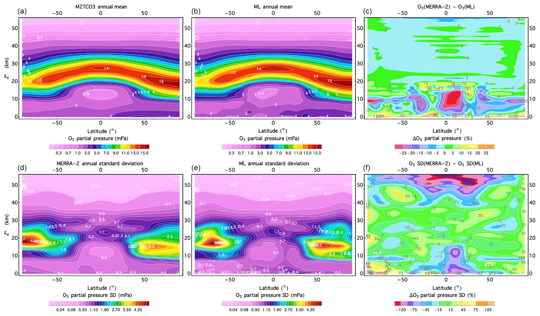
Figure 14 Annual zonal mean profiles and standard deviations from M2TCO3 and ML climatologies and their differences. (a, b, c) Latitude-dependent O₃ partial pressure (mPa) profiles: M2TCO3 (a), ML (b), and their relative differences (c). (d, e, f) Latitude-dependent O₃ profile standard deviations (mPa): M2TCO3 (a), ML (b), and their percent differences (c).

The baseline climatologies constructed from MERRA-2 data describe the systematic behavior of the O₃ profile and variance and their spatial and temporal dependence on tropopause pressure and total O₃ column. Since there is no other O₃ profile climatology with a similar resolution and dependency, we validated the MERRA-2 climatologies by downgrading and then comparing them with independent climatological data sets. In Sect. 4.2, we validated the daytime tropopause-dependent (downgraded in LST and longitude) M2TPO3 climatology, which shows good agreement with the TPO3 climatology (Sofieva et al., 2014) compiled from independent O₃ profile data. In Sect. 4.6, we validated the spatiotemporal O₃ variations represented in the downgraded (in LST and O₃ columns) daytime M2TCO3 climatology, which shows good agreement with the Ziemke2011 and GLiu2013 climatologies. In this section, we present further comparisons of vertical profiles and integrated quantities (i.e., vertical columns) to demonstrate the validity of the M2TCO3 climatology.

We compare the daytime annual zonal mean (i.e., downgraded in LST, season, longitude, and O₃ column) M2TCO3 climatology with the annual zonal mean (downgraded in season) ML climatology (McPeters and Labow, 2012), which is an improved version of the LLM climatology (McPeters et al., 2007). Figure 13 shows the annual mean O₃ profiles (panels a and b) and their standard deviations (panels d and e) as functions of altitude and latitude from the daytime M2TCO3 and ML climatologies. This figure also includes the plots of the relative (percent) difference between the mean profiles (panel c) and between the standard deviations (panel f) from these two climatologies. In the upper stratosphere ($Z^{*}>\mathrm{20}$ km), annual mean profiles have an excellent agreement between these two climatologies, with relative differences mostly within ±3 % (see Fig. 13a–c). However, relative differences are larger but within ±30 % in the lower stratosphere and troposphere ($Z^{*}<\mathrm{20}$ km), mainly due to sampling differences and due to the lack of tropospheric O₃ production in the MERRA-2 reanalysis (Wargan et al., 2015; Bosilovich et al., 2015). These differences between M2TCO3 and ML climatologies are within the uncertainties estimated from the differences between two climatologies compiled from different sources, including the ML and the LLM in McPeters and Labow (2012), the TPO3 and the ML, and the TPO3 and the LLM in Sofieva et al. (2014).

As shown in Fig. 13d–f, the standard deviations of the downgraded M2TCO3 climatology are similar to those of the ML climatology: both capture the high variability in the upper troposphere and lower stratosphere (UTLS) and the low variability in the upper stratosphere, with a vast majority of differences within ±30 %. The sampling differences contribute to the standard deviation differences exhibited in Fig. 13f.

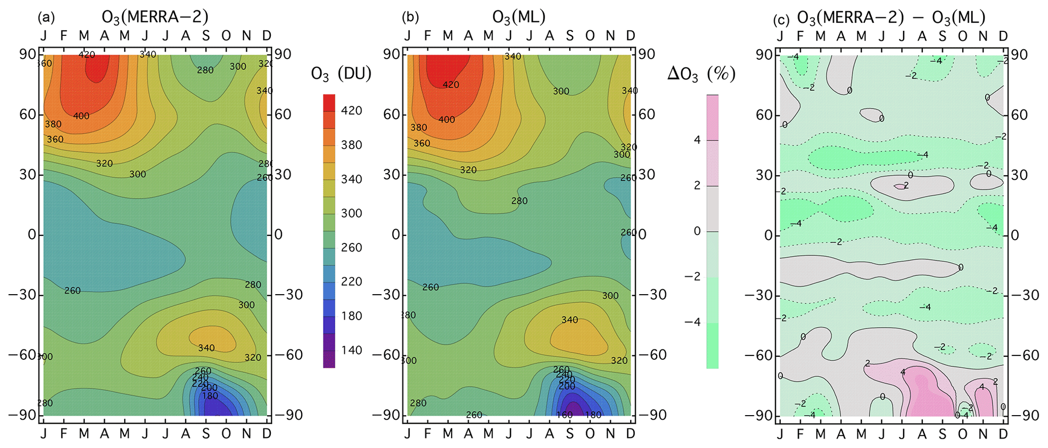
Figure 15 Comparison of monthly zonal mean total column O₃ from the daytime M2TCO3 (a) and the ML (b) climatologies and their relative differences (c). Both climatologies capture the strong annual cycle of total O₃, which exhibits a maximum in late winter–early spring in the NH and a minimum in late summer–early fall in the SH.

Figure 14 shows the total O₃ columns versus month and latitude from the ML and the downgraded M2TCO3 climatologies and their percent differences, illustrating the good agreements between the two for a vast majority of months and latitude zones, with O₃ absolute differences less than 4 %. Absolute differences exceeding 4 % occur in a few areas only, notably in the northern polar zone for several months during which M2TCO3 total columns are lower than those of ML by more than 4 %, and in the SH above 70^∘ latitude for the months from August to December during which M2TCO3 total columns are higher than those of ML by more than 4 %. These large biases likely result from spatially inhomogeneous O₃ distributions, such as the longitudinally and seasonally dependent tropospheric O₃ distributions (Ziemke et al., 2011; Liu et al., 2013) and the strong O₃ gradient across the Antarctic ozone hole, which are sampled differently in creating the two climatologies. While the MERRA-2 assimilation provides a spatially and temporally uniform O₃ field, the ozonesonde stations distributed unevenly around the globe provide intermittent O₃ profile measurements, and the MLS on the polar-orbiting Aura platform samples more densely at higher latitudes. As a result, the ML climatology, which relies on the ozonesonde data and the Aura MLS O₃ profile measurements, samples each latitude zone unevenly, thus contributing to the differences in Fig. 14.

In summary, comparisons of climatological profiles and standard deviations between M2TPO3 and TPO3 (see Figs. 4 and 5), annual zonal mean profiles and standard deviations between M2TCO3 and ML (see Fig. 13), and integrated monthly zonal mean profiles (i.e., the total column O₃) between M2TCO3 and ML (see Fig. 14) show good overall agreement, with differences similar to those between two climatologies constructed from different data sources, thus validating the daytime M2TPO3 and daytime M2TCO3 climatologies.

6 Conclusions

Tropopause-pressure-classified (M2TPO3) and total-ozone-column-classified (M2TCO3) climatologies are created from the MERRA-2 O₃ profile record between 2005 and 2016, within the period of Aura MLS and OMI assimilation. The enormous number of MERRA-2 O₃ profile data that cover the globe uniformly and continuously enable precise and accurate representations of systematic behaviors and dynamical variations in O₃ vertical distributions. The resulting set of O₃ profiles and covariance matrices captures their dependence on longitude, latitude, local solar time, and season, as well as on tropopause pressure or O₃ abundance, more accurately over a broader range and at a higher resolution than other O₃ profile climatologies. Parameterization of O₃ profile with tropopause pressure or total column O₃ reduces the variability in stratosphere and troposphere compared to the month–latitude-dependent climatology, therefore providing improved a priori knowledge of O₃ vertical distribution. Both M2TPO3 and M2TCO3 climatologies contain quantitative information about O₃ profile covariances, which is not included in previous O₃ profile climatologies. The profile covariances provide more realistic constraints on O₃ profile retrievals based on the OE inversion technique. Moreover, the EOFs of the climatological covariance matrices facilitate a new scheme to represent the O₃ profile and guide a retrieval algorithm to successively improve O₃ profile user information contained in spectral measurements.

For profile retrieval algorithms, a closer match between actual and a priori O₃ profiles, especially in the region where spectral measurements have low vertical resolution, improves the retrieval accuracy. Thus tropopause-dependent O₃ climatology, which reduces the variability further in the UTLS region, is more appropriate for use with O₃ profile algorithms. However, the variability reduction is overall higher with column O₃ parameterization, indicating more realistic O₃ profile assignment based on total column abundance. Therefore the column-dependent O₃ climatology is uniquely suited for use in total O₃ retrieval algorithms, as the retrieved column determines the likely O₃ vertical distribution without needing additional information.

The M2TCO3 climatology provides improved O₃ profile representation, capturing systematic profile changes resulting from column variations and their dependence on season and spatial location, which are missing from or insufficiently represented by previous column-classified climatologies (e.g., Wellemeyer et al., 1997; Bhartia and Wellemeyer, 2002; Lamsal et al., 2004; Labow et al., 2015) with coarse latitude and time resolutions. The smooth profile change between adjacent dependent variables (illustrated in figures in Appendix A) implies that merging profiles from different columns, months, and tiles can provide spatially and temporally continuous representation of the O₃ profile. The MERRA-2 temperature climatology and the M2TCO3 climatology are used in the O₃ and SO₂ combination algorithm applied to retrievals from DSCOVR EPIC (EPIC Science Team, 2018), SNPP OMPS-NM (Yang, 2017), and Aura OMI. The description and validation of these O₃ and SO₂ products will be presented in separate papers.

Appendix A: Figures of the MERRA-2 O₃ and temperature profile climatologies

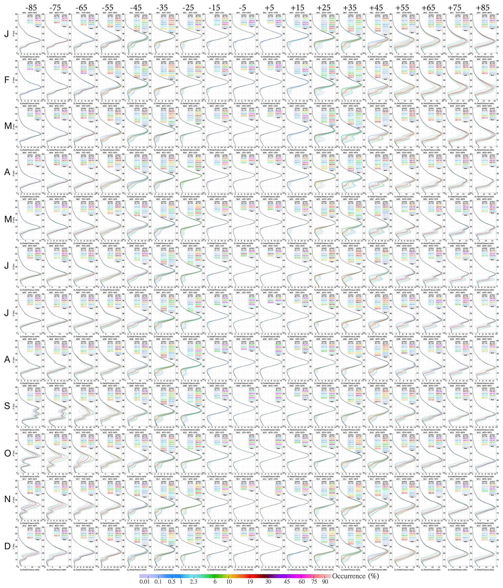
Figure A1 The daytime M2TPO3 climatology contains 2154 O₃ profiles that are distributed among the 12×18 month–latitude classes. The color of a solid line indicates the percentage occurrence of the profile. The line legends display the average tropopause altitudes and the average total O₃ columns. The solid gray line represents the downgraded M2TPO3 profile, i.e., the monthly zonal mean profile.

Figure A2 Similar to Fig. A1, except for profile standard deviations in daytime M2TPO3 climatology. This illustrates that tropopause pressure classification in general reduces the variability of the climatological profile.

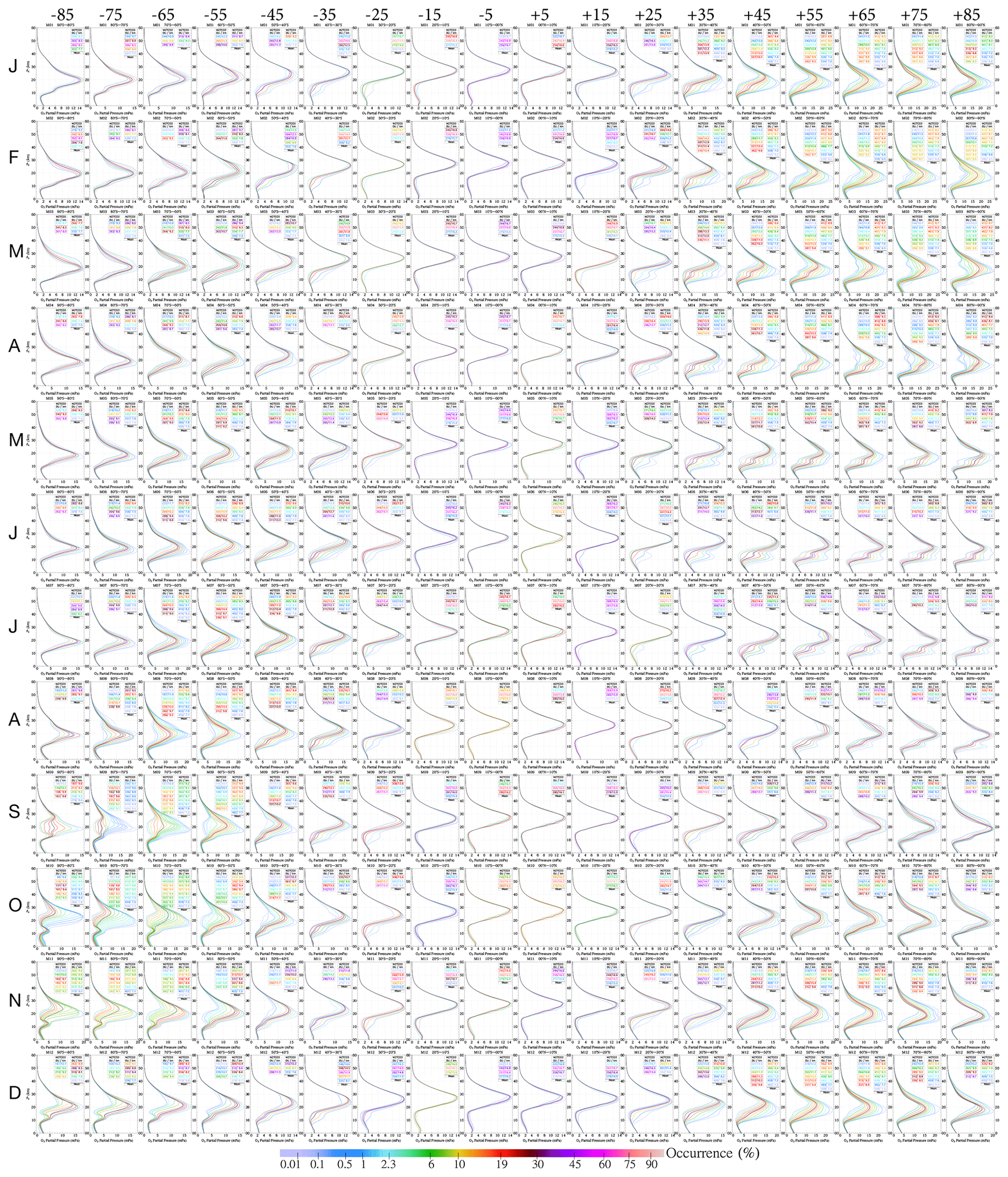
Figure A3 The daytime M2TCO3 climatology contains 1644 O₃ profiles that are distributed among the 12×18 month–latitude classes. The color of a solid line indicates the percentage occurrence of the profile. The line legends display the average tropopause altitudes and the average total O₃ columns. The solid gray line represents the downgraded M2TCO3 profile, i.e., the monthly zonal mean profile.

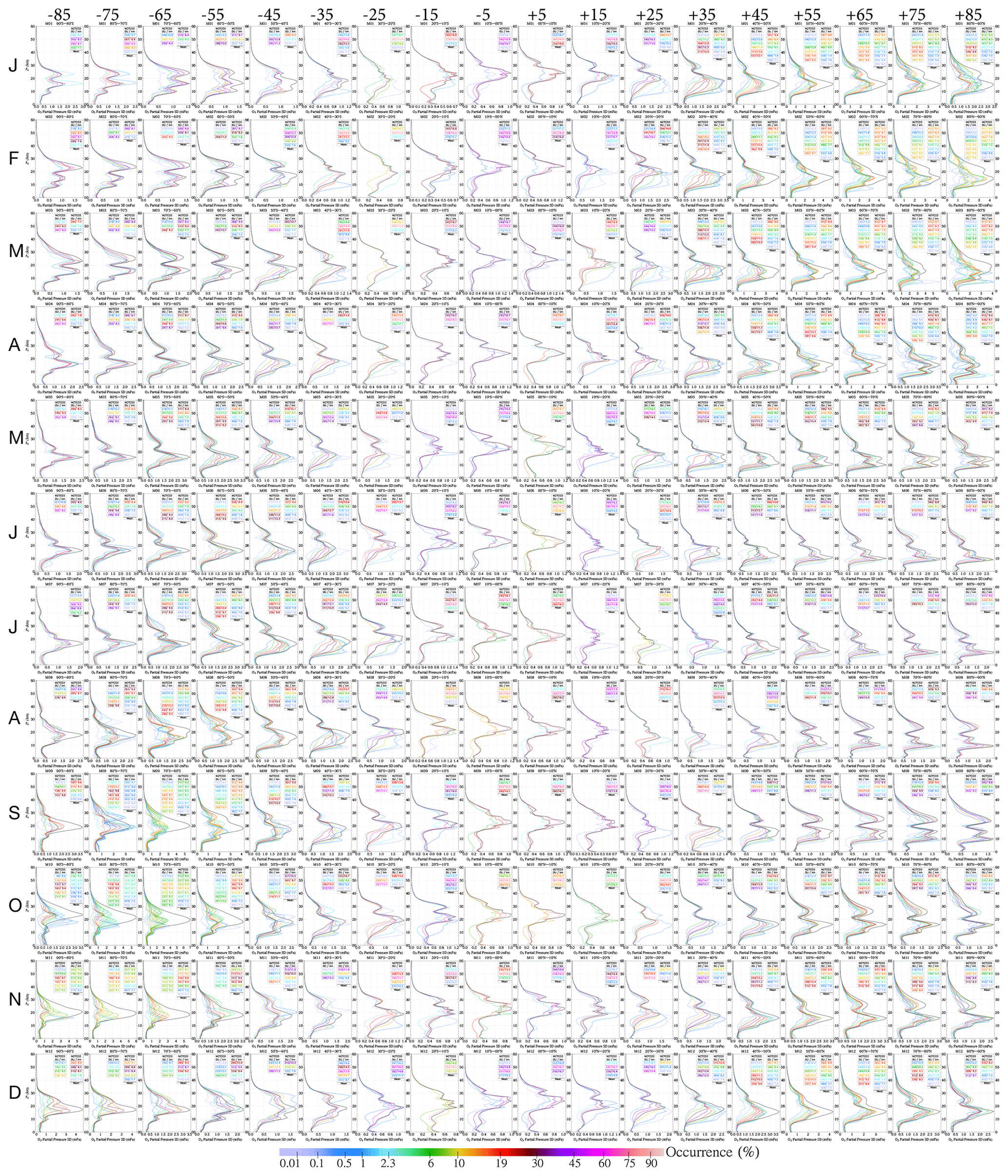
Figure A4 Similar to Fig. A3, except for profile standard deviations in daytime M2TCO3 climatology. This illustrates that total O₃ column classification in general reduces the variability of the climatological profile.

Figure A5 O₃ profile correlation matrices corresponding to daytime monthly zonal mean profiles. The correlation matrices are standardized or normalized covariance matrices (with 1 s in the main diagonal).

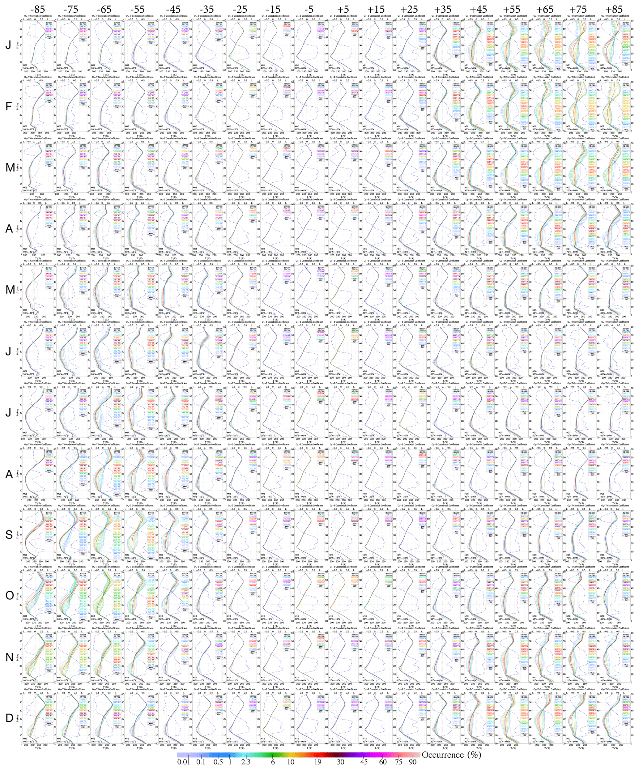
Figure A6 Climatological temperature profiles corresponding to the daytime M2TCO3 O₃ profiles shown in Fig. A3. The color scheme is the same as that in Fig. A3. The dashed dark blue line represents the coefficient of correlation between O₃ partial pressure and temperature as a function of pressure altitude Z^*.

The baseline climatologies consist of statistics of MERRA-2 O₃ and temperature profiles collected from 24×18 rectangular tiles at eight different UTC times each separated by 3 h. Since each tile has the size of 15^∘ longitude by 10^∘ latitude, the tile statistics at a UTC represent the statistics of an hour of local solar time. Combining the statistics of different tiles within a range of local solar time downgrades the baseline climatologies to month–latitude (i.e., no distinction in longitude) climatologies, as illustrated in this paper with the example of daytime (09:00–17:00) climatologies. Similarly morning, afternoon, or nighttime climatologies may be created by selecting the proper local solar time range in combining tiles with the same latitude zone.

In this appendix, each O₃ profile in the daytime M2TPO3 and the daytime M2TCO3 climatologies and the corresponding profile variance are displayed in Figs. A1 to A4, which show O₃ partial pressure or standard deviation (mPa) as a function of pressure altitude Z^* from 0 to 71 km (or 1013.25 to 0.04 hPa). Colored solid lines represent the climatological profiles in Figs. A1 and A3 or the corresponding standard deviations in Figs. A2 and A4. The color of a solid line indicates the percentage occurrence of the climatological profile, and the line legend displays the average tropopause altitude and the average total column O₃. The solid gray line represents the downgraded (monthly zonal mean) profile in Figs. A1 and A3 or the corresponding standard deviations in Figs. A2 and A4. Panels in each row show change with latitude, while those in each column reflect seasonal variation.

The MERRA-2 climatologies contain quantitative characterizations of O₃ profile covariances. Correlation matrices, which are normalized covariance matrices, associated with daytime monthly zonal means are shown in Fig. A5.

Accompanied by the O₃ profile climatologies, temperature profile climatologies are created. Figure A6 shows the climatological temperature profiles associated with the daytime M2TCO3 climatology. Figure A6 includes the monthly zonal O₃–temperature correlation profiles to illustrate the consistent correlation pattern for all latitude zones and seasons.

Appendix B: Climatology usage

Interpolation

The MERRA-2 baseline climatologies provide local-solar-time-dependent coverage over the globe with equally sized (15^∘ longitude × 10^∘ latitude) tiles, which are quite coarse compared to the spatial resolutions of most spaceborne observations. For retrieval applications, the a priori information for a specific time and location may be determined from climatological data via spatial and temporal interpolation to ensure continuous representation in time and space. Frequently, the baseline climatologies are downgraded in longitude to generate the latitude-zone-dependent climatologies (e.g., see Figs. A1 and A3). A retrieval application using these latitude-zone-dependent climatologies usually performs temporal and latitudinal interpolation to provide time- and location-dependent a priori information.

Setting a climatological profile to a user-specified total column

Frequently, an O₃ retrieval algorithm needs to set a climatological profile X to a specific total column Ω. For the M2TPO3 climatology, this is accomplished by finding the coefficient ω₁, such that the profile integration of

$$\begin{array}{}\text{(B1)}& \mathbf{X}={\mathbf{X}}_{\mathrm{m}}+{\mathit{\omega }}_{\mathrm{1}}{\mathbf{e}}_{\mathrm{1}}\end{array}$$

is equal to Ω. For the M2TCO3 climatology, this can be done by linear interpolation or extrapolation of the column-dependent climatological profile X_m(Ω₁) and X_m(Ω₂),

$$\begin{array}{}\text{(B2)}& \mathbf{X}=w_{\mathrm{1}}{\mathbf{X}}_{\mathrm{m}}\left({\mathrm{\Omega }}_{\mathrm{1}}\right)+w_{\mathrm{2}}{\mathbf{X}}_{\mathrm{m}}\left({\mathrm{\Omega }}_{\mathrm{2}}\right),\end{array}$$

where Ω₁ and Ω₂ are the two climatological columns that are closest to Ω, and the coefficients $w_{\mathrm{1}}=({\mathrm{\Omega }}_{\mathrm{2}}-\mathrm{\Omega })/({\mathrm{\Omega }}_{\mathrm{2}}-{\mathrm{\Omega }}_{\mathrm{1}})$ and $w_{\mathrm{2}}=(\mathrm{\Omega }-{\mathrm{\Omega }}_{\mathrm{1}})/({\mathrm{\Omega }}_{\mathrm{2}}-{\mathrm{\Omega }}_{\mathrm{1}})$. When Ω is too far (−15 DU > or >15 DU) outside the valid M2TCO3 range, Eq. (B1) with X_m and e₁ from the M2TCO3 climatology may be used to set the profile X to the desired total column Ω.

The O₃ column used in selecting a profile from the M2TCO3 climatology refers to the total column from profile integration down to the sea level ($Z^{*}=\mathrm{0}$ km). When the bottom level of a user-defined vertical grid is significantly above the sea level, such as the cases over the Himalayan Plateau or Antarctica, the column from the integration of the user grid needs to add the climatological column from the bottom level to the sea level for profile selection from the M2TCO3 climatology.

Mapping of a climatology to a user-defined vertical grid

The baseline climatologies contain O₃ concentration (i.e., mixing ratio) profiles specified at m=72 equally spaced pressure altitude levels ($Z^{*}=\mathrm{0}$ to 71 km by 1 km) and their covariance matrices. Frequently an O₃ retrieval application needs to recast the concentration profiles and their covariance matrices into those of column amount of the vertical layers. Next, we describe the equations for mapping a level-based climatology to user-defined atmospheric layers.

Given an atmospheric layering scheme, it is straightforward to convert a mixing ratio profile X into a column density profile Ψ of n layers $\mathit{\{}{\mathrm{\Psi }}_j=X_j{A}_j,j=\mathrm{1},\mathrm{\dots },n\mathit{\}}$, where X_j is the mean mixing ratio of the jth layer, and A_j is the layer air column density, which is determined by the difference between pressures at the layer boundaries. Usually, X_j is determined via interpolation or extrapolation (if a user grid is outside the grid range of the climatology) from X.

An m×m covariance matrix S_m, which is real and symmetric by definition, may be decomposed exactly as

$$\begin{array}{}\text{(B3)}& {\mathbf{S}}_m=\mathbf{Q}\mathbf{\Lambda }{\mathbf{Q}}^T,\end{array}$$

where $\mathbf{Q}=[{\mathbf{e}}_{\mathrm{1}},{\mathbf{e}}_{\mathrm{2}},\mathrm{\dots },{\mathbf{e}}_m]$ is an orthogonal matrix of m columns, with its ith column e_i being the ith eigenvector of the covariance matrix S_m, and $\mathbf{\Lambda }=\mathrm{diag}({\mathit{\lambda }}_{\mathrm{1}},{\mathit{\lambda }}_{\mathrm{2}},\mathrm{\dots },{\mathit{\lambda }}_m)$ is a diagonal matrix, with its ith element λ_i being the ith eigenvalue of S_m. Similar to converting a mixing ratio profile into a layer column density profile, the eigenvectors $\mathit{\{}{\mathbf{e}}_i,i=\mathrm{1},\mathrm{\dots },m\mathit{\}}$, also known as the empirical orthogonal functions (EOFs), are converted into layer column density vectors, $\mathit{\{}{{\mathbf{e}}^{\prime }}_i,i=\mathrm{1},\mathrm{\dots },m\mathit{\}}$, and the elements of the ith column vector are $\mathit{\{}{e}_{ij}^{\prime }=e_{ij}{A}_j,j=\mathrm{1},\mathrm{\dots },n\mathit{\}}$, where e_ij is the mean value of e_i at layer j, usually obtained through interpolation or extrapolation from e_i. The n×n layer-to-layer covariance matrix S_n is constructed as

$$\begin{array}{}\text{(B4)}& {\mathbf{S}}_n={\mathbf{Q}}^{\prime }\mathbf{\Lambda }{{\mathbf{Q}}^{\prime }}^T,\end{array}$$

where ${\mathbf{Q}}^{\prime }=[{{\mathbf{e}}^{\prime }}_{\mathrm{1}},{{\mathbf{e}}^{\prime }}_{\mathrm{2}},\mathrm{\dots },{{\mathbf{e}}^{\prime }}_m]$ is a matrix of m column vectors, each with the length of n.

A covariance matrix example

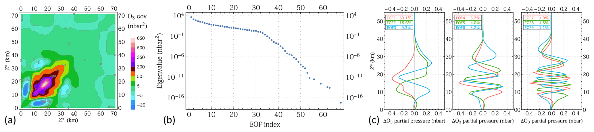
Figure B1 (a) The covariance matrix for October and the midlatitude (50–40^∘ S) zone, (b) eigenvalues of the covariance matrix in (a), and (c) the first nine leading EOFs of the matrix in (a).

We show an example of a covariance matrix S_m in Fig. B1a, its eigenvalues in Fig. B1b, and the nine leading EOFs in Fig. B1c. The eigenvalues drop rapidly with higher index i (see Fig. B1b) and are typically between 15 and 20 leading EOFs to account for 99 % of the total variances. The S_n may be reconstructed with a smaller number (<m) of leading EOFs in Eq. (B2). Doing so may reduce the total variance represented by S_n, thus improving the numerical stability of O₃ profile retrievals that use S_n as an a priori constraint.