Microwave Radar/radiometer for Arctic Clouds (MiRAC): first insights from the ACLOUD campaign

The Microwave Radar/radiometer for Arctic Clouds (MiRAC) is a novel instrument package developed to study the vertical structure and characteristics of clouds and precipitation on board the Polar 5 research aircraft. MiRAC combines a frequency-modulated continuous wave (FMCW) radar at 94 GHz including a 89 GHz passive channel (MiRAC-A) and an eight-channel radiometer with frequencies between 175 and 340 GHz (MiRAC-P). The radar can be flexibly operated using different chirp sequences to provide measurements of the equivalent radar reflectivity with different vertical resolution down to 5 m. MiRAC is mounted for down-looking geometry on Polar 5 to enable the synergy with lidar and radiation measurements. To mitigate the influence of the strong surface backscatter the radar is mounted with an inclination of about 25^∘ backward in a belly pod under the Polar 5 aircraft. Procedures for filtering ground return and range side lobes have been developed. MiRAC-P frequencies are especially adopted for low-humidity conditions typical for the Arctic to provide information on water vapor and hydrometeor content. MiRAC has been operated on 19 research flights during the ACLOUD campaign in the vicinity of Svalbard in May–June 2017 providing in total 48 h of measurements from flight altitudes >2300 m. The radar measurements have been carefully quality controlled and corrected for surface clutter, mounting of the instrument, and aircraft orientation to provide measurements on a unified, geo-referenced vertical grid allowing the combination with the other nadir-pointing instruments. An intercomparison with CloudSat shows good agreement in terms of cloud top height of 1.5 km and radar reflectivity up to −5 dBz and demonstrates that MiRAC with its more than 10 times higher vertical resolution down to about 150 m above the surface is able to show to some extent what is missed by CloudSat when observing low-level clouds. This is especially important for the Arctic as about 40 % of the clouds during ACLOUD showed cloud tops below 1000 m, i.e., the blind zone of CloudSat. In addition, with MiRAC-A 89 GHz it is possible to get an estimate of the sea ice concentration with a much higher resolution than the daily AMSR2 sea ice product on a 6.25 km grid.

1 Introduction

In the rapidly changing Arctic climate (e.g., Serreze et al., 2009; Graversen et al., 2008), the role of clouds and associated feedback remain unclear (Osborne et al., 2018; Wendisch et al., 2017). In particular, understanding the effect of mixed-phase clouds whose persistence is controlled by a complex interaction of microphysical, radiative, and dynamic processes is still challenging (Morrison et al., 2012). Information on their vertical structure and phase partitioning, which control their radiative impact (Curry et al., 2002), is currently available from the few ground-based profiling sites in the Arctic, e.g., Utqiaġvik (formerly known as Barrow), Alaska (Shupe et al., 2015); Ny-Ålesund, Svalbard (Nomokonova et al., 2019); and Summit, Greenland (Shupe et al., 2013). The use of synergistic lidar and cloud radar measurements is key for the study of these cloud systems. Passive microwave measurements further provide information on the vertically integrated liquid water path (LWP). The profiling sites provide important long-term statistics; however, they might be limited in their representativity for the wider Arctic.

Polar-orbiting passive satellite imagery provides coverage of the Arctic region; however, the retrieval of cloud properties is challenged by the surface properties and suffers from limited vertical information. Active spaceborne measurements by lidar and radar, i.e., by the combination of Cloud-Aerosol Lidar and Infrared Pathfinder Satellite Observation (Winker et al., 2003, CALIPSO) and CloudSat (Stephens et al., 2009), have been fundamental in better understanding the vertical structure of clouds around the globe. However, the CloudSat Cloud Profiling Radar (CPR) provides limited information in the lowest 0.75 to 1.25 km due to the presence of strong surface echo (Maahn et al., 2014; Burns et al., 2016), while the CALIPSO lidar observations are often fully attenuated by the presence of supercooled liquid layers. Using CALIPSO and CloudSat measurements Mioche et al. (2015) identified the region around Svalbard to be particularly interesting to study mixed-phase clouds as these show a higher frequency of occurrence (55 %) here compared to the Arctic average (30 % in winter and early spring, 50 % May to October).

Airborne platforms have the advantage of high spatial flexibility and accessibility of remote places comparable to satellite observations. While a number of airborne campaigns have been performed in the Arctic since the 1980s (Andronache, 2017; Wendisch et al., 2018), the use of a radar–lidar system in these aircraft campaigns is rather limited. One notable exception was during the Polar Study using Aircraft, Remote Sensing, Surface Measurements and Models, of Climate, Chemistry, Aerosols, and Transport (POLARCAT) campaign in spring 2008, in which Delanoë et al. (2013) studied an Arctic nimbostratus ice cloud using the French airborne radar–lidar instrument in detail.

During May–June 2017 the Arctic CLoud Observations Using airborne measurements during polar Day (ACLOUD; Wendisch et al., 2018; Knudsen et al., 2018) aircraft campaign was performed as part of the ArctiC Amplification: Climate Relevant Atmospheric and SurfaCe Processes, and Feedback Mechanisms project ((AC)³; Wendisch et al., 2017). The research aircraft Polar 5 and 6 of the Alfred Wegener Institute (AWI) operating from Longyearbyen, Svalbard, deployed a remote sensing and in situ microphysics instrument package, respectively. Polar 5 was equipped with the Airborne Mobile Aerosol Lidar for Arctic research (AMALi; Stachlewska et al., 2010) and spectral solar radiation measurement already operated during the VERtical Distribution of Ice in Arctic clouds (VERDI; Schäfer et al., 2015) campaign. During ACLOUD, the remote sensing package was complemented by the novel Microwave Radar/radiometer for Arctic Clouds (MiRAC). In contrast to most other millimeter radars employed on research aircraft (e.g., Radar Aéroporté et Sol de Télédétection des propriétés nuAgeuses, RASTA; Delanoë et al., 2012; High-performance Instrumented Airborne Platform for Environmental Research (HIAPER) Cloud Radar, HCR; Rauber et al., 2017; Wyoming Cloud Radar, WCR; Khanal and Wang, 2015; High Altitude and LOng range research aircraft Microwave Package, HAMP; Mech et al., 2014), which use short microwave pulses for ranging, the radar of the MiRAC package employs a frequency-modulated continuous wave (FMCW) radar. Thus, a lower peak power transmitter is used; however, careful consideration on handling the surface return is required. Therefore, in the past, airborne FMCW radar has been mounted in uplooking geometry (Fang et al., 2017).

The purpose of this study is twofold. First, the MiRAC package, which consists of a unique 94 GHz FMCW radar (MiRAC-A) and an eight-channel passive microwave radiometer with channels between 170 and 340 GHz (MiRAC-P), is introduced. The instrument specifications and integration into the Polar 5 aircraft in downward-looking geometry are provided in Sect. 2 followed by the methodology used to quality control and map the observations to a geo-referenced coordinate system in Sect. 3. The performance of MiRAC during its first deployment within ACLOUD will be demonstrated via a comparison with CloudSat within a case study in Sect. 4, and a short statistical analysis of the ACLOUD measurements is shown in Sect. 5. Conclusions and outlook to further analysis and deployments of MiRAC are given in Sect. 6.

2 Instruments and aircraft installation

MiRAC is composed of an active (MiRAC-A) and passive (MiRAC-P) part. MiRAC-A is mounted between the wings of the research aircraft Polar 5 and MiRAC-P is mounted inside of the aircraft measuring through a sufficiently large aperture (see Fig. 3). Since the FMCW radar needs a different measuring angle, MiRAC-A is tilted by 25^∘ backwards with respect to nadir, whereas MiRAC-P is nadir-looking. The following three sections will describe the instruments and aircraft installation in detail.

2.1 FMCW W-band radar

MiRAC-A is based on the novel single vertically polarized cloud radar RPG-FMCW-94-SP manufactured by RPG-Radiometer Physics GmbH, which is described in detail by Küchler et al. (2017). It basically consists of a transmitter with adjustable power to protect the receiver from saturation, a Cassegrain two-antenna system for continuous signal transmission and reception, and a receiver containing both the radar receiver channel at 94 GHz and the passive broadband channel at 89 GHz. To guarantee accurate measurements both channels are thermally stabilized within a few millikelvin. The FMCW principle allows us to achieve high sensitivity for short-range resolutions down to 5 m with low transmitter power of about 1.5 W from solid state amplifiers. The radar is also equipped with a passive channel at 89 GHz using the same antenna as the radar. The radar has been calibrated to provide the equivalent radar reflectivity Z_e with an uncertainty of 0.5 dBz. The uncertainty of the brightness temperature (TB) measured by the 89 GHz channel is ±0.5 K (Küchler et al., 2017).

The cloud radar was originally developed for ground-based application. Here the passive channel is especially useful because liquid water strongly emits at 89 GHz, and with the cosmic background temperature as a low and well-known background signal the LWP can be derived from TB measurements. As explained in the next subsection the strong and highly variable emissivity of the surface complicates LWP retrieval from the airborne perspective. However, it additionally provides information about the presence of sea ice exploited from satellite (Spreen et al., 2008).

For the installation on the Polar 5 aircraft, the radar’s antenna aperture size had to be reduced from 500 mm down to 250 mm in order to accommodate the radar into the Polar 5 belly pod. This implies a sensitivity loss of 6 dB compared to the original RPG-FMCW-94-SP design. The smaller antenna size implies a wider half power beam width (HPBW) of 0.85^∘ (antenna gain approx. 47 dB). The quasi bistatic system’s 90 % beam overlap (beam separation of 298 mm) is achieved at a distance of 75 m from the radar (compared to 280 m for the 500 mm aperture radar). Therefore, measured Z_e profiles start at 100 m distance from the aircraft.

In the case of aircraft deployments, the radar’s receiver can be easily run into saturation caused by strong ground reflections when pointing toward the nadir, due to the fact that a FMCW radar continuously emits and receives signal power. A pulsed radar overcomes this problem because the strong ground reflection pulse does not affect the atmospheric reflection signals, which are received delayed in time relative to the ground pulse. Therefore, the antenna axis of a down-looking FMCW radar deployed on an aircraft must be tilted against the nadir axis, so that the ground reflection becomes significantly attenuated. A comprehensive analysis of sufficient inclination viewing angles relative to nadir for FMCW radar observations is given in Li (2005). The Polar 5 radar has been tilted by 25^∘ from nadir backwards, following the guidelines in Li et al. (2005).

For a FMCW radar, ranging is achieved by transmitting sawtooth chirps with continuously increasing transmission frequency over a given sampling time and frequency bandwidth. The time difference between transmission and reception of a given frequency provides the range resolution. If the radar signal is backscattered by a particle moving towards or away from the radar, an additional frequency shift much smaller than one from ranging occurs due to the Doppler effect. The Doppler spectrum for each range gate yields from the radar processing involving two fast Fourier transformations (FFTs). For an airborne radar the Doppler spectrum is difficult to interpret due to the Doppler effect induced by aircraft motion (Mech et al., 2014). Although we can apply de-aliasing techniques to unfold the Doppler velocity, the results have not been satisfying so far. It has been found out that background wind information is needed to disentangle the Doppler velocity from the aircraft motion. Such information is not available on board Polar 5. Therefore, we make only use of the equivalent radar reflectivity factor Z_e in this study, which can be determined from the integral over the Doppler power spectrum.

During ACLOUD two different chirp sequences per profile defining the vertical resolution and thus minimum detectable Z_e (Z_min) were used to account for the fact that the sensitivity of the radar receiver decreases with the distance squared. For the very first flights of MiRAC a conservative vertical resolution was chosen to ensure a high enough sensitivity even if unforeseen problems would arise. With a range resolution of 17.9 m over the first 500 m (Sequence I in Table 1) Z_min decreases from −65 dBz at 100 m distance from aircraft to about −50 dBz at a distance of 600 m (Fig. 1). Using a second chirp sequence with a coarser range resolution of 27 m for the rest of the profile improves Z_min, which then again degrades with the distance squared, reaching roughly −45 dBz at the surface for the typical flight altitude of 3 km above ground (Fig. 1). Encouraged by the well-behaved performance of MiRAC with these conservative settings during the first flights, the chirp sequences were modified to yield a higher vertical resolution of 4.5 m in the first 500 and 13.5 m for the rest of the flights (Sequence III in Table 1). Note that due to higher flight altitudes the chirp settings had to be adapted (Sequence II in Table 1) to still cover the full column during limited periods.

Table 1 Chirp settings and corresponding range resolution for the different research flights (RFs). MiRAC has been operated on 19 RFs.

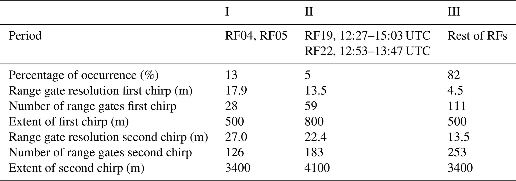
Figure 1 exemplarily illustrates the actually achieved Z_min for three research flights with the different chirp settings. Herein, Z_min is calculated for each range gate by integrating over the noise power of the Doppler spectrum. Under typical atmospheric conditions this results in the classical behavior discussed above. However, Fig. 1 shows that sometimes deviations can occur which are due to the two following reasons. First, the Doppler spectrum noise power computation fails if the spectral width exceeds the range gate’s maximum Nyquist velocity. This situation occurs in range gates affected by the strong surface reflectivity and causes the enhanced occurrence of Z_min up to −20 dBz. Due to different flight altitudes, e.g., clustered around 3.2 km for the example in Fig. 1I, enhanced Z_min associated with the surface is spread over different range gates. Second, the parallel shifts of Z_min profiles are caused by the automatic transmitter power level switching. The radar automatically levels the transmitter power in cases when the input power might lead to receiver saturation effects. The signal power reduction then leads to reduced sensitivity over the whole profile. The automatic power reduction is triggered by high reflections, which can occur under certain flight conditions, e.g., during flight maneuvers leading to a nadir viewing of the radar and thus increased surface backscatter.

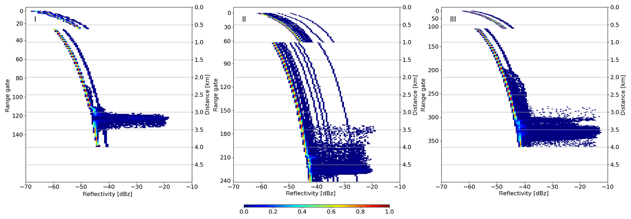
Figure 1 Sensitivity limit (dBz) (Z_min) for vertical polarization of different chirp tables with different vertical resolution as a function of distance from the aircraft (secondary y axes) for the three settings used during ACLOUD. The vertical resolution increases from left to right (I to III) with increasing number of range gates: (I) 154 range gates, 25 May, 08:58–12:19 UTC, RF05; (II) 242 range gates 23 June, 12:53–13:43 UTC, RF22; (III) 364 range gates 27 May, 08:14–11:04 UTC, RF06.

2.2 Passive millimeter and submillimeter radiometer

The passive microwave radiometer MiRAC-P (or RPG-LHUMPRO-243-340) is a unique instrument combining millimeter and submillimeter channels that has been never operated before and especially not in the Arctic and on an aircraft. In contrast to the MiRAC radar, the passive microwave channels deployed on the Polar 5 aircraft are pointing toward the nadir with respect to the aircraft fuselage. In order to co-align radar and passive observations, the atmospheric signal delay caused by the radar tilt must be taken into account by correcting for the aircraft’s horizontal speed. For reference, a detailed description of MiRAC-P is provided below.

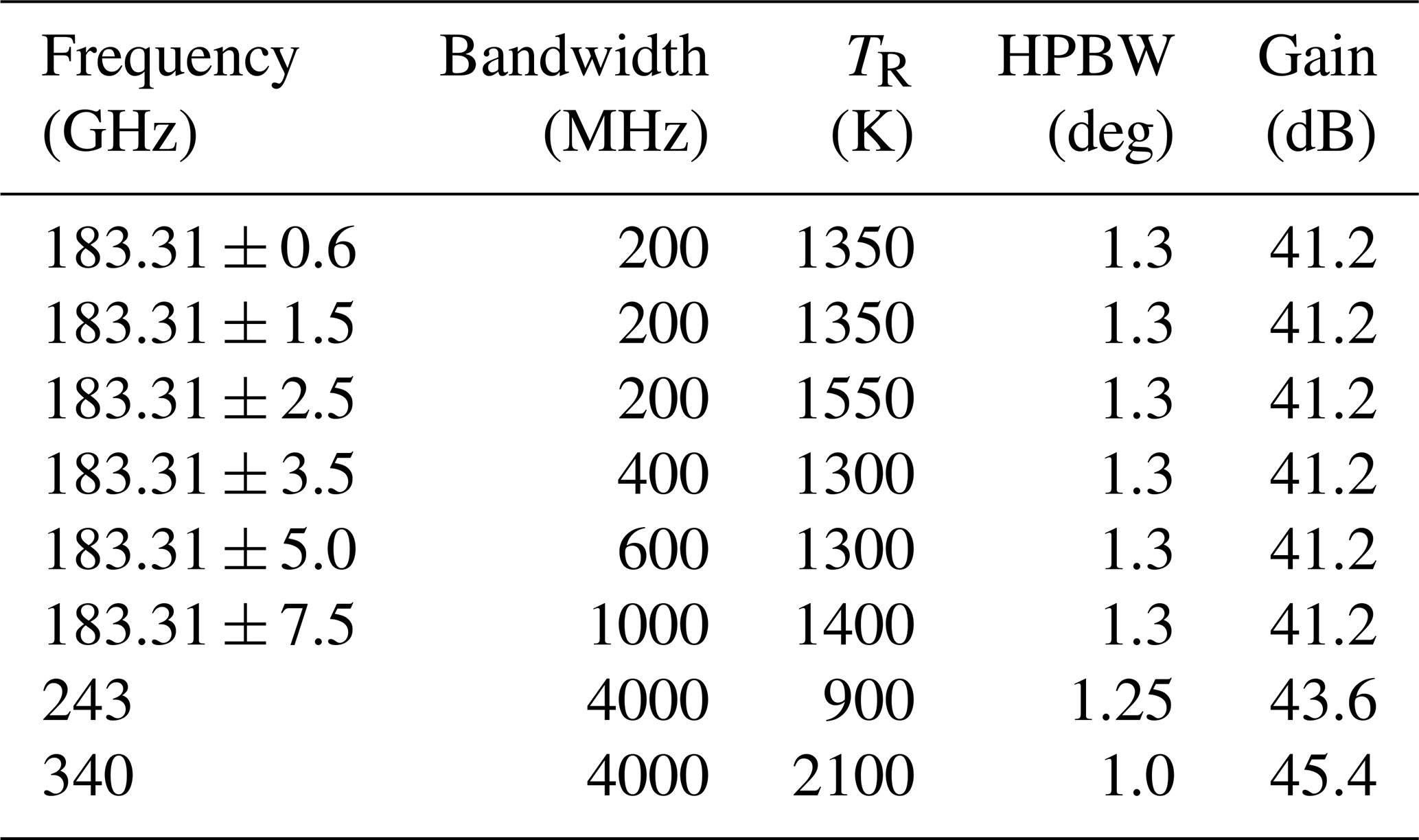
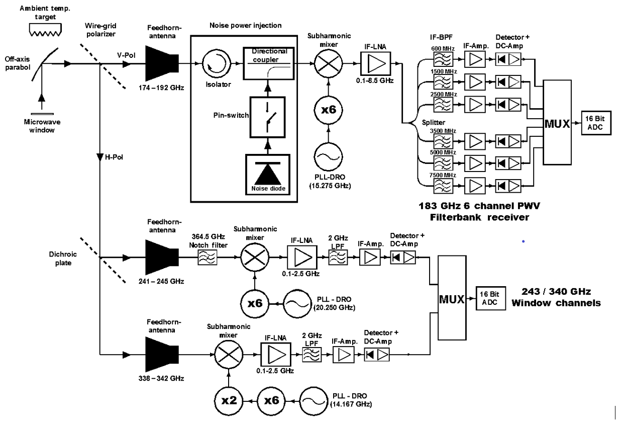
MiRAC-P consists of a double sideband (DSB) receiver with six channels centered around the 183.31 GHz water vapor (WV) line and two window channel receivers at 243 and 340 GHz. The schematic in Fig. 2 shows the overall system layout. The received radiation enters the radiometer through a low loss radome window (attenuation at 180 GHz approx. 0.01 dB) and is then reflected by an off-axis parabola antenna onto a wire grid beam splitter, forming beams between 1.3 and 1^∘ (Table 2). The vertical polarization is transmitted into the 183.31 GHz water vapor receiver (WVR) while the horizontal polarization is further split in frequency by a dichroic plate, separating the 243 from the 340 GHz channel. All receivers are of DSB heterodyne type utilizing subharmonic mixers as the frontal element. The local oscillators (LOs) consist of phase-locked loop (PLL) stabilized fundamental dielectric resonant oscillators (DROs), multiplied by several active frequency multiplier stages as shown in Fig. 2. The frequency stability of these oscillators is close to 10⁻⁷ K⁻¹.

Table 2 Specifications of MiRAC-P.

The WVR is equipped with a secondary standard, a noise-switching system periodically injecting a precise amount of white noise power to the receiver input. By assuming a stable constant noise power over time, receiver gain fluctuations are effectively canceled (noise-adding radiometer; see Ulaby et al., 1981). Unfortunately, state-of-the-art noise sources with reasonable power output of at least 13 dB excess noise ratio are currently limited to maximum frequencies around 200 GHz, so that the two window channels (243 and 340 GHz) cannot use and benefit from them.

The WVR’s intermediate frequency (IF) architecture is a six-channel filter-bank design with the characteristics given in Table 2. All channels are acquired simultaneously (100 % duty cycle) by using a separate detector for each channel with 1 s temporal resolution. The window channel’s IF bandwidth (BW) is 1950 MHz for both 243 and 340 GHz. Because of the DSB mixer response, this corresponds to twice as much signal bandwidth of about 4 GHz (Table 2) having a small gap of 100 MHz in the center. Both sidebands are combined in the mixer IF output signal, so that a flat mixer sideband response is essential, meaning the mixer sensitivity and conversion loss must be almost identical in both sidebands. The subharmonic mixer design is optimal in this respect, offering a sideband conversion loss balance of better than 0.1 dB. The most demanding receiver in terms of sideband balance is the WVR due to its overall signal bandwidth of 15 GHz. The benefit of the DSB receiver design is a more than doubled radiometric sensitivity compared to a SSB (single sideband) receiver.

The parabolic mirror at the optical input can be turned to all directions for scanning purposes (sky view) or to point to the internal ambient temperature precision calibration target (accuracy 0.2 K). The WVR uses this target to determine drifts in receiver noise temperature while the 243 and 340 GHz channels are correcting for gain drifts. Typically, calibration cycles are repeated automatically every 10 to 20 min by the radiometer's internal control PC. These long intervals are possible because of a dual stage thermal control system, stabilizing the receiver's physical temperatures to better than 30 mK over the whole environmental temperature range (−30 to +45 ^∘C). Given the receiver noise temperatures T_R (Table 2) and the integration time of 1 s, measurement noise is below 0.5 K.

Figure 2 Block diagram of MiRAC-P.

2.3 Installation and aircraft operation

The Polar 5 aircraft is a Basler BT-67 operated by the Alfred Wegener Institute for Polar and Oceanic Research (Wesche et al., 2016). In addition to MiRAC, the AMALi lidar and radiation sensors were integrated into the Polar 5. To provide accurate information on the aircraft position, an inertial navigation system is used, which provides information on aircraft orientation, i.e., pitch ϵ, roll ρ, and heading η angles, as well.

Due to the simpler electronic design and lack of high-voltage components compared to pulsed systems, the FMCW radar has relatively small dimensions of 83 cm × 57 cm × 42 cm and a weight of 88 kg allowing a relatively simple integration into the Polar 5 aircraft. As cabin space and openings are limited a special belly pod has been designed to accommodate MiRAC-A (Fig. 3) below the aircraft. The belly pod with a size of 200 cm × 89 cm × 50 cm has been designed and fabricated by Lake Central Air Services. Openings of 27 cm in diameter for the transmitter and receiver antennas allow an unstopped view of MiRAC exposing the radomes directly to the environment. When grounded the aircraft fuselage is tilted by roughly 14^∘ and the radar is integrated in the belly pod such that the pointing is about 25^∘ backward during typical flight operation. The exact mounting position of the radar with respect to the aircraft is derived by a calibration method, which requires a calibration flight pattern, in which roll and pitch angle as well as flight altitude are changed rapidly over calm ocean. Further insight of determining the mounting position is described in Sect. 3.2.

In contrast to the radar MiRAC-A, MiRAC-P is integrated to Polar 5 roughly pointing at nadir during the flight. While in ground-based operation MiRAC-P can be mounted on a stand with the microwave transparent radome oriented towards zenith (Rose et al., 2005), here the radiometer box is fixed head over directly to the floor of the aircraft cabin (Fig. 3) looking through an opening in the fuselage. In this way the radome is directly exposed to the air avoiding any attenuation. In order to co-align radar and passive observations, the atmospheric signal delay caused by the radar tilt must be taken into account by correcting for the aircraft's horizontal speed. To protect the instruments during start and landing, the instrument compartment including MiRAC-P underneath the Polar 5 is protected via flexible roller doors.

For both passive components, MiRAC-P and the receiver at 89 GHz of MiRAC-A, absolute calibrations with liquid nitrogen have to be performed before the first flight after the installation as described in Rose et al. (2005) and Küchler et al. (2017). This procedure has to be repeated whenever the instruments are without power for a longer period or are flown in significantly different conditions. On ground the instruments are constantly heated to keep conditions stable for the receiver parts.

MiRAC has been operated successfully on 19 research flights (RF) during the ACLOUD field experiment with significant data loss occurring only during RF13 on 5 June 2017 due to software problems. Though some flights were flown close to the ground for albedo and flux measurements, more than 50 % of the flight time was dedicated to straight legs above 2300 m altitude (pitch angle ϵ<10^∘ and roll $\left|\mathit{\rho }\right|<\mathrm{3}$^∘) allowing us to probe a large range of different cloud conditions, e.g., over ocean, the marginal sea ice zone, and closed ice (Fig. 4). A special focus has been put on flights in the vicinity of the research vessel Polarstern that set up an ice-floe camp northwest of Svalbard in the framework of the Physical feedback of Arctic boundary layer, Sea ice, Cloud and AerosoL (PASCAL) campaign (Wendisch et al., 2018) between 5 and 14 June 2017.

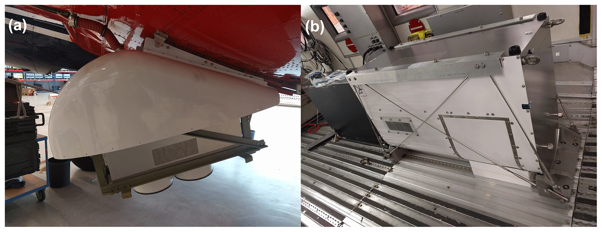
Figure 3 (a) MiRAC-A with opened belly pod below the research aircraft Polar 5. (b) MiRAC-P eight-channel radiometer mounted in the aircraft cabin.

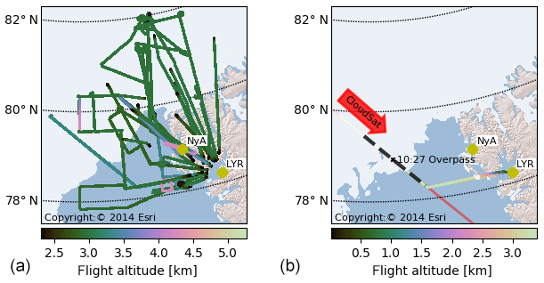
Figure 4 (a) Tracks of all research flights of Polar 5 during ACLOUD around Svalbard with an altitude h (above sea level) larger than 2.3 km, ϵ<10^∘, and $\left|\mathit{\rho }\right|<\mathrm{3}$^∘. (b) Polar 5 CloudSat underflight on 27 May between 10:06 and 10:44 UTC west of Svalbard. In red the CloudSat track is shown. The white colored area shows the 15 % sea ice coverage derived from AMSR2 observations.

3 Data processing

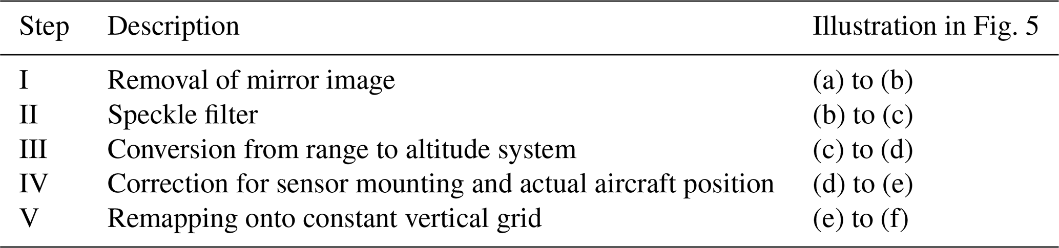
In total five processing steps convert the raw data to the final geo-referenced data product (Table 3). First, a methodology to identify and remove range side-lobe artifacts induced by the strong surface echo return is developed (Sect. 3.1) and applied to the MiRAC-A observations on its native coordinate system. Second, W. C. Lee et al. (1994) provide an explicit analytical method to map data from aircraft-relative to Earth-relative coordinates. Here, we extended their method to fit our purpose (Sect. 3.2). All variables measured by MiRAC are recorded in the sensor-relative coordinate system. For scientific analysis, however, data with geographic coordinates longitude λ, latitude ϕ, and altitude h are needed. All processing steps are illustrated in Fig. 5 for an exemplary radar reflectivity time series.

Table 3 Processing steps for MiRAC-A radar measurements

3.1 Filtering of range side-lobe artifacts

The filtering described here identifies and removes non-meteorological artifacts in the radar reflectivity observations induced by range side lobes. The slant distance of the aircraft to the surface can easily be identified from the range gate with the strongest Z_e, which is associated with the surface return. The strength of the surface radar return depends on the type of surface (i.e., land, sea ice, broken sea ice, or open water) and wind speed. The FFT of piecewise continuously differentiable functions lead to overshooting waves at discontinuities. This phenomenon is called Gibbs phenomenon (Gibbs, 1899; Gottlieb and Shu, 2003). The Gibbs phenomenon explains the range side lobes appearing near the strong surface radar reflectivity signal. The effect depends on the filter characteristics of the FFT used in signal processing, which typically produce symmetric side lobes. While range gates above the surface can include contributions from both the atmosphere and the surface, the “mirror signal” below the surface is only produced by the leakage of the surface return. This is illustrated for a 1 h time series in Fig. 5a. Clearly a side lobe is visible in range gates below the surface, especially in the first part of the flight over sea ice (see Fig. 7 for sea ice cover) with similar characteristics in the corresponding range gates above the surface. Hence, there are two horizontal disturbance lines in time, which are “mirrored” at the surface signal. The second part of the flight leg is less affected, which can be attributed to a change in surface characteristics of the marginal sea ice zone and open water.

The processing step I (Table 3) includes the removal of the mirror image, which is also called subsurface reflection filter in Table A1 of the Appendix. Herein, the below-surface range side lobe is quantified and subsequently subtracted from both range side lobes. For this subtraction of the mirror signal we assume that both range side lobes above and below the surface are equal, which is justified by the symmetry of the digital FFT filter function. The subtraction method is defined by considering the environment of every single time step. At each time step three measurements before and after are considered to locate the subsurface reflection, the mirrored signal below the surface, and its vertical extent. Within the located subsurface reflection the value of the highest disturbance is used as the subtracted value. The extent of the subsurface reflection and its distance from the highest reflectivity signal of the surface to the center of the subsurface reflection provides the distance to locate the range side lobe and its extent above the surface.

However, as illustrated in Fig. 5b some scattered radar reflectivities still remain. Thus, processing step II (Table 3) applies a speckle filter that removes isolated signals either remaining from the insufficient mirror image correction that does not take into account higher harmonics or due to other processing artifacts. Most important thin isolated horizontal disturbance lines evident in Fig. 5b need to be eliminated. The speckle filtering is based on the procedure by J. S. Lee et al. (1994). However, the filter is simplified by considering a radar reflectivity mask, which is defined by setting all radar reflectivities to 1 and everything else to 0. Then, the filter uses a box considering all neighboring measurements around a centered pixel. At a chosen threshold preferably close to 50 % of ones, the centered value will be set to 0 or will be kept as 1. The aim of the filtering procedure is to remove single speckle pixel and horizontal disturbance lines, which may remain after processing step I. Thus, the box should be as small as possible and should have a rectangular shape tilted by 90^∘ to the horizontal disturbance line comparable to the side lobes. The value for the time range is chosen as 3 because it is the smallest value with a centered time step. Conversely, the range gate range must be much larger than the time range, but also an odd number. The observations show that the maximum extent of the disturbance line has an extent of five to six pixels in range gate direction. Having a filtering threshold of 50 % in mind, the size of the box corresponds to 11 or 13 range gates. Taking 13 range gates for the box gives a better opportunity to fit the threshold to the optimal exclusion of speckle and horizontal disturbance lines. Thus, empirical estimations lead to a threshold of 41.7 %. However, a slight data loss at cloud boundaries is obvious by using such a filter. Figure 5c shows the result of the filtering procedure, which excludes speckle and horizontal disturbance lines.

Close to the surface the contamination by the surface reflection is too high to apply a correction. Therefore the lowest 150 m to the surface needs to be ignored (Fig. 5f, grey shading). Further information of the filtered values can be found in the Appendix (Table A1).

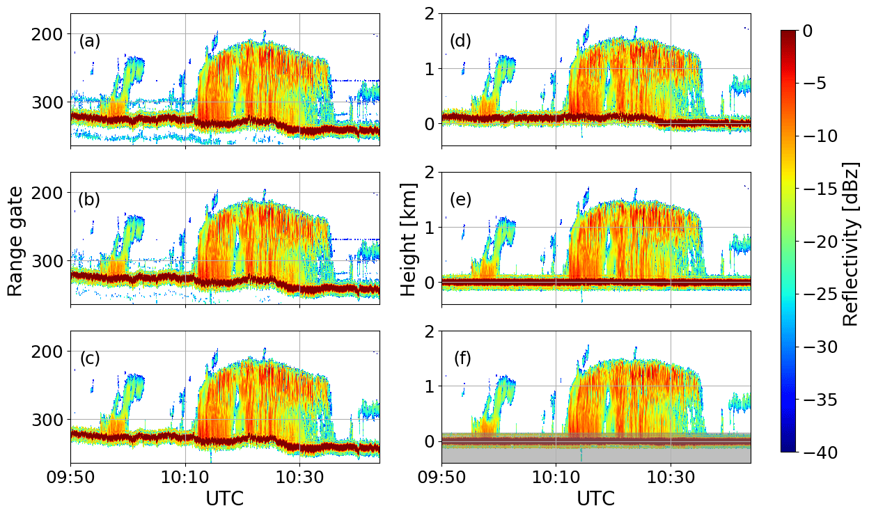
Figure 5 Time series of Z_e profiles measured during RF06 on 27 May 2017 for different processing steps (see Table 3): (a) raw data; (b) after subtraction of mirror signal; (c) after speckle filter; (d) filtered data on a time–height grid; (e) corrected for sensor altitude, mounting position, pitch, and roll angle; and (f) remapped onto a constant vertical grid. The grey shading indicates the range of surface contamination (≤150 m).

3.2 Coordinate transformation

For the conversion of the measurements into the geographical coordinate system the approach by W. C. Lee et al. (1994) is extended and generalized. Two additional frames of reference are introduced: first, the sensor-related coordinate system, in which the data are recorded and which is not identical to the platform (airframe) coordinates, and, second, the global geographic coordinate (λ, ϕ, h) system, which is used in many applications and is of equal interest as the local Earth-relative coordinate (local east, north, zenith) system.

Then, the technique by establishing a mathematical object called transform that performs coordinate transformations between different reference frames is generalized. It can be inverted and composed, providing a simple formalism for multistep coordinate transformations. Furthermore, it can be easily implemented in object-oriented programming languages. The generalization comes at the expense of a slightly elevated level of abstractness. A detailed description is provided in the Appendix.

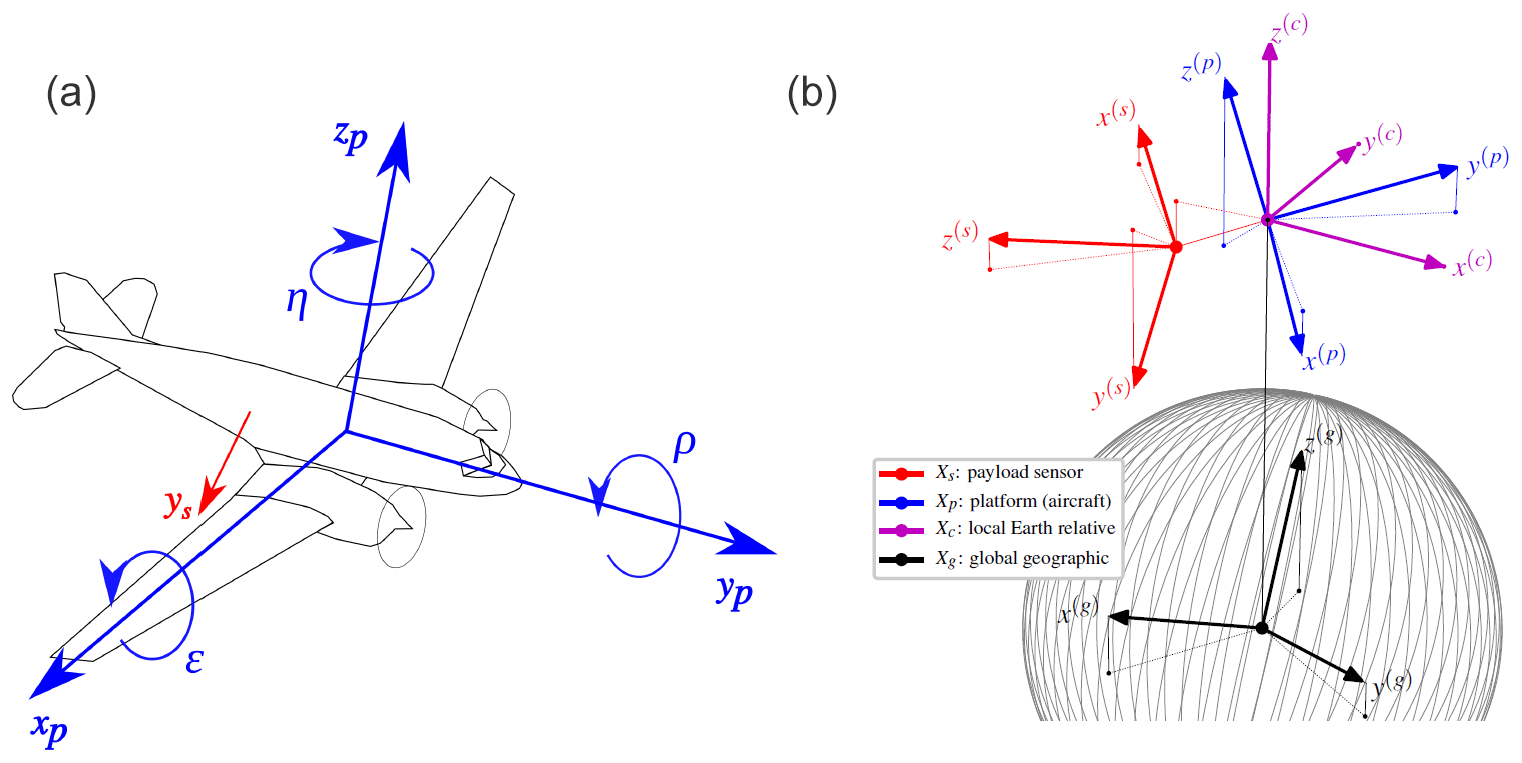
Figure 6 (a) Sketch of the Polar 5 aircraft and the platform-relative X_p reference frame. (b) Reference frames for airborne measurements: sensor-relative X_s (red), platform-relative X_p (blue), local Earth-relative X_c (purple), and global geographic (black). The grey lines are meridians of X_g and the sphere they indicate may be seen as the planet surface, but distances are obviously not to scale. In blue are coordinate axes of the aircraft reference frame X_p and principal rotation angles: heading η, pitch ϵ, and roll ρ. In red is the y axis of X_s.

The coordinate transformation from the payload sensor-relative reference frame X_s to the global geographic reference frame X_g, i.e., processing step III (Table 3), is done via two intermediate reference frames. First, the coordinates are transformed from X_s to the platform-relative reference frame X_p. Then a transformation to the local Earth-relative reference frame X_c is performed. Finally, the coordinates are transformed from X_c to X_g. The origins and orientations of the reference frames are defined in Table 4 and visualized in Fig. 6. If possible, the definitions of W. C. Lee et al. (1994) are adopted.

Table 4 Positions and orientations of the reference frames. The x and y axes of X_g are defined in the common way: x_g points towards the intersection of the Equator and the prime meridian and the y_g in the direction that completes the right-handed perpendicular coordinate system. Note that X_c is not located on the planet's surface but on the platform.

The mathematical basis of the coordinate transformation and its application is described in detail in the Appendix (A). Basically the mathematical operators T_ij called transforms are defined, which allow the simple conversion from one coordinate system into the next. In processing step IV (Table 3; Fig. 5d to e) the exact mounting of the sensor within the aircraft and the actual positioning of the aircraft are determined.

The parameters that define T_sp, i.e., the transformation from the sensor to the platform reference frame, are the location and orientation of the payload sensor within X_p. Within the sensor installation (Sect. 2.3) these parameters were only known with moderate uncertainties (±0.5 m and ±3^∘, respectively). Assuming that the position and attitude sensors of the Polar 5 operate on much higher precision, the other two transforms T_pc and T_cg are much more precise. The overall precision is thus limited by T_sp. To get the precise sensor installation parameters, a calibration routine is developed. The calibration is performed over calm ocean or shallow sea ice in order to get a sharp discontinuity of the surface echo. Furthermore clouds should not be too thick, so that the surface return of the radar is the strongest signal of the profile. The calibration assumes that the altitude of the signal maximum is the surface reflectivity return, which is at an altitude of 0 m. Due to variations in position and attitude of the platform, this is extremely unlikely to happen consistently when using wrong parameters.

A suitable time interval of 2.5 h over calm ocean surface is considered and the downhill-simplex algorithm of Nelder and Mead (1965) is applied. The algorithm is used to minimize the cost function $c=\sum _i{\mathit{\zeta }}_i^{\mathrm{2}}$. This yields the position and attitude of the payload sensor relative to X_p. ζ_i is the altitude (in X_g) of the signal maximum at time step i and c is ideally equal to 0. However in practice, the minimum reachable value is bounded by the finite width of the sensor's range gates. Using this calibration, c can be improved by a factor of 3. In particular the attitude of the payload sensor has a large impact on the transformed target altitude. Using the same technique, offsets in the interpretation of time readings between the payload, position, and sensors attitude are detected in fractions of a second. These offsets affect c because T_pc and T_cg are time dependent.

The performed calibration of the $z_{\mathrm{s}}^{\left(\mathrm{p}\right)}$ coordinate of the sensor position, the sensor attitude, and the time offset technique is stable with respect to changes of the first guess in a domain of reasonable estimates and the time interval chosen for the calibration. The parameters $x_{\mathrm{s}}^{\left(\mathrm{p}\right)}$ and $y_{\mathrm{s}}^{\left(\mathrm{p}\right)}$ show only very little effect on c. This is expected since most of the time they are close to orthogonal with respect to zenith. When including them in the calibration, the algorithm still converged in all investigated cases, but much slower.

Finally, the last processing step V (Table 3) shows the result of the remapping that interpolates the data onto a constant vertical grid. Herein the time shift of the tilted profile to a true vertical column is considered, allowing an easy combination with the nadir-pointing MiRAC-P, lidar, and radiation data. The processed reflectivity data product is publicly available (Kliesch and Mech, 2019).

4 Case study

One of the objectives of the ACLOUD campaign is the evaluation of satellite products in the Arctic (Wendisch et al., 2018). Here, the added value of airborne radar observations is highlighted in this example of a CloudSat underflight that took place over the Arctic ocean northwest of Svalbard (Fig. 4). A roughly 30 min flight leg centered around the exact overpass time at 10:27 UTC at 78.925^∘ N and 2.641^∘ E is shown in Fig. 7 together with the corresponding CloudSat measurements. Note that this stretch is also included in the processing example of Fig. 5, which allows a more detailed look into the MiRAC radar measurements, which provides more than a factor of 10 finer vertical resolution (<30 m) compared to the CloudSat 250 m data product. Note that the resolution associated with the CloudSat pulse length is 485 m (Stephens et al., 2009). In terms of spatial resolution the 1.4 (1.8) km cross track (along track) of CloudSat roughly corresponds to 30 MiRAC measurements (15 depending on aircraft speed).

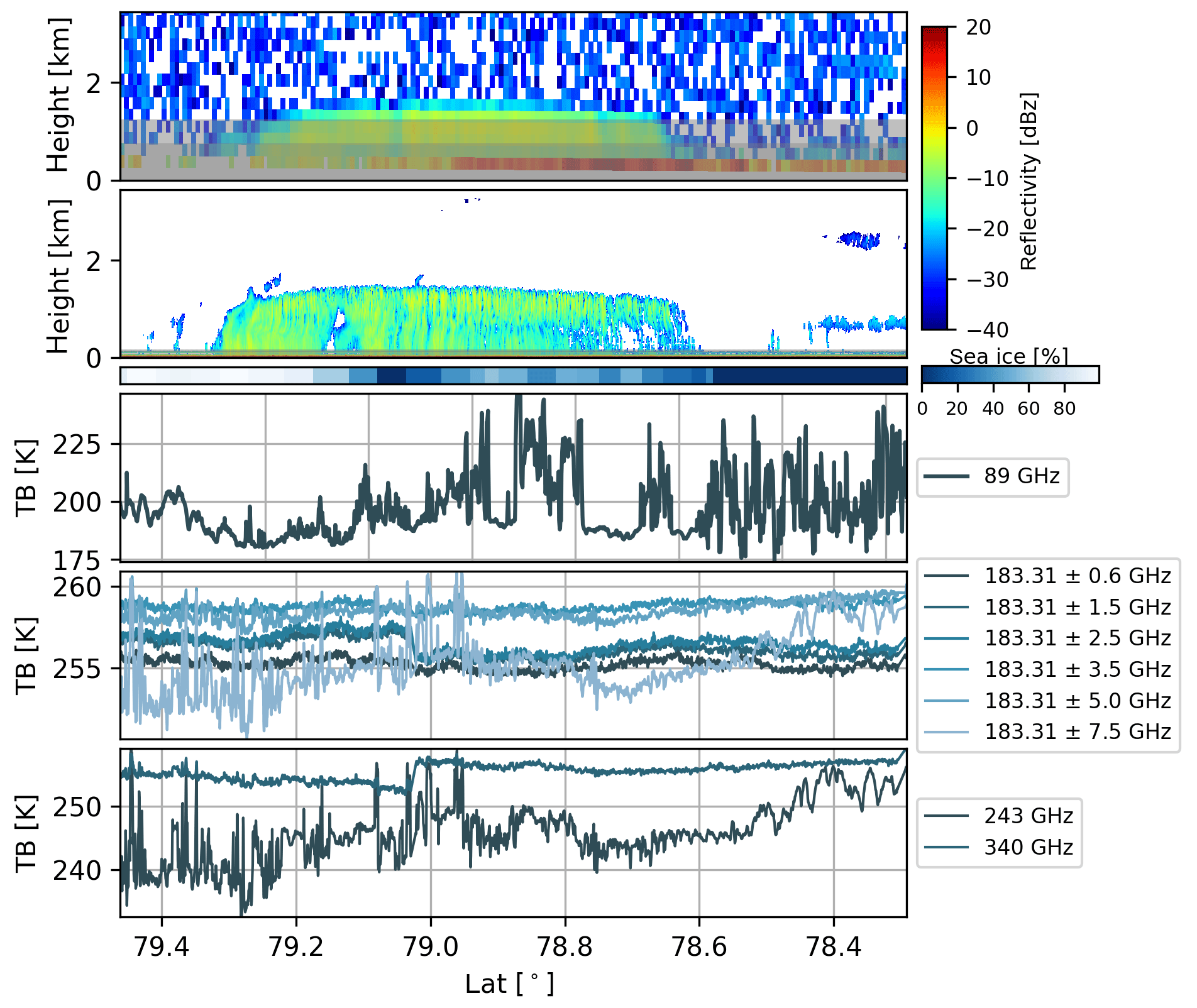
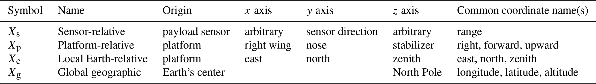
Figure 7 Vertical cross section of Z_e measured by CloudSat CPR (top) and the MiRAC radar on Polar 5 (second row) for the satellite underflight on 27 May 2017 between 10:06 and 10:44 UTC along the black dashed line in Fig. 4. Grey shaded areas define the zone of reduced sensitivity. The third row gives the sea ice coverage based on AMSR2 observations along the flight track. Rows four to six show the passive radiometer measurements at 89 GHz from MiRAC-A and those channels of MiRAC-P, i.e., the six channels along the 183.31 GHz water vapor absorption line, and the two channels at 243 and 340 GHz.

The measurements are taken from a leg when the Polar 5 was flying southeast passing through the marginal sea ice zone towards the open ocean, which is reached roughly at 78.6^∘ N as indicated by the sea ice product derived from the Advanced Microwave Scanning Radiometer (AMSR2) by the University of Bremen (Spreen et al., 2008). The transition from 100 % sea ice fraction in the beginning of the flight leg to open ocean at the end of the track is nicely seen by the change in the radar surface return, which significantly increases in the vertical-pointing CPR measurements close to the surface (Fig. 7). Note that here the surface-contaminated range gates, i.e., blind zone, have not been eliminated. For MiRAC the lowest 150 m needs to be omitted while for CloudSat the nominal blind zone is about 0.75 to 1.25 km depending on the surface echo strength (Tanelli et al., 2008). Nevertheless, the CPR detects the precipitating cloud system with maximum cloud top height of 1.6 km rather consistently in its spatial extent of 150 km with MiRAC. In terms of reflectivity the CPR indicates slightly higher average values, especially in the more southern part over ocean, which however might result from additional surface contamination. Due to the low cloud top height, we refrain from looking at height averaged Z_e profiles as done by Delanoë et al. (2013) for the case of a 5 km high nimbostratus cloud. As shown in Fig. 5 MiRAC is able to resolve the individual patches of enhanced reflectivities associated with turbulent processes as well as smaller-scale clouds. Additional underflights were performed with CloudSat; during ACLOUD unfortunately no CPR measurements are available due to satellite problems.

The daily AMSR2 sea ice product with 6.25 km spatial resolution mainly relies on TB measurements at 89 GHz. Such measurements are available with much finer resolution from MiRAC-A's passive 89 GHz channel. As can be seen in the beginning of the flight track, strong fluctuations in this channel between roughly 190 and 240 K mirror a strong change in surface emissivity (Fig. 7) with the lowest values being consistent with open water while higher TBs indicate ice. These high-frequency fluctuations are consistent with visual observations that reveal a high degree of brokenness in the sea ice. Towards the end TB stays at lower values typical for ocean surfaces before they increase again, however, with much smoother behavior than during the broken sea ice conditions. This increase can be attributed to liquid water emission by the thin (dz=350 m) cloud shown by the radar at roughly 800 m height, which can not be resolved by the CPR.

Time series of MiRAC-P TB clearly identify optically thick channels, which are not affected by the surface by their relatively constant behavior during the complete flight leg (Fig. 7). The first channel at 183±0.6 GHz being closest to the strong water vapor absorption shows the coldest TB as its emission stems from water vapor at higher altitudes. With channels moving farther away from the line center, channels successively receive radiation from lower layers as the emission stems from lower atmospheric layers. At a certain point along the line the atmosphere becomes transparent and surface emission also contributes to TB. This can be best seen for the outermost 183±7.5 GHz and the window channel at 243 GHz. This channel is of particular interest as it will also be flown on the Ice Cloud Imager (ICI; Kangas et al., 2014) on board MetOp-SG to be launched in 2023. Scattering by ice particles strongly increases with increasing frequency and therefore a brightness temperature depression can occur. Disentangling the contribution of water vapor, liquid water, the surface, and ice scattering is complex and is part of the ongoing retrieval development.

5 Cloud statistics

MiRAC as a remote sensing suite has been operated on Polar 5 during ACLOUD on 19 research flights summing up to more than 80 flight hours. In a first analysis macroscopic cloud properties are derived for the whole flight campaign. For that purpose the processed reflectivities (Sect. 3) measured from flight altitudes of at least 2300 m and with small aircraft pitch and role angles (ϵ<10 and $\left|\mathit{\rho }\right|<\mathrm{3}$^∘) are considered. This results in 52 % of the total flight time along the tracks shown in Fig. 4 being usable for the analysis. Due to the orography of Svalbard, radar measurements are difficult to interpret. Therefore, measurements over land are excluded. Most of the time Polar 5 was flying at an altitude of about 2900 to 3000 m, which can be seen in Fig. 8 as well where about 80 % of all measurements considered in the statistical analysis were acquired with this flight altitude or above. Figure 8 and Table 5 also show that about 57 % of the measurements were taken over open ocean and 43 % over sea ice. It has to be kept in mind that flight patterns were planned to observe clouds according to numerical weather prediction models. Therefore, the statistics might be biased.

Figure 8 Height-dependent cloud top height and cloud fraction (CF) on intervals of 100 m. The interval center is written in the y ordinate. (a) number of measurements; (b) solid lines describe the total averaged cloud fraction at each height over all profiles; box–whisker plots of cloud fraction averaged over 20 min with percentiles of 10 %, 25 %, 50 %, 75 %, and 90 % from left to right; (c) cumulative occurrence of averaged cloud top height. The sea ice fraction is derived from satellite observations by AMSR2.

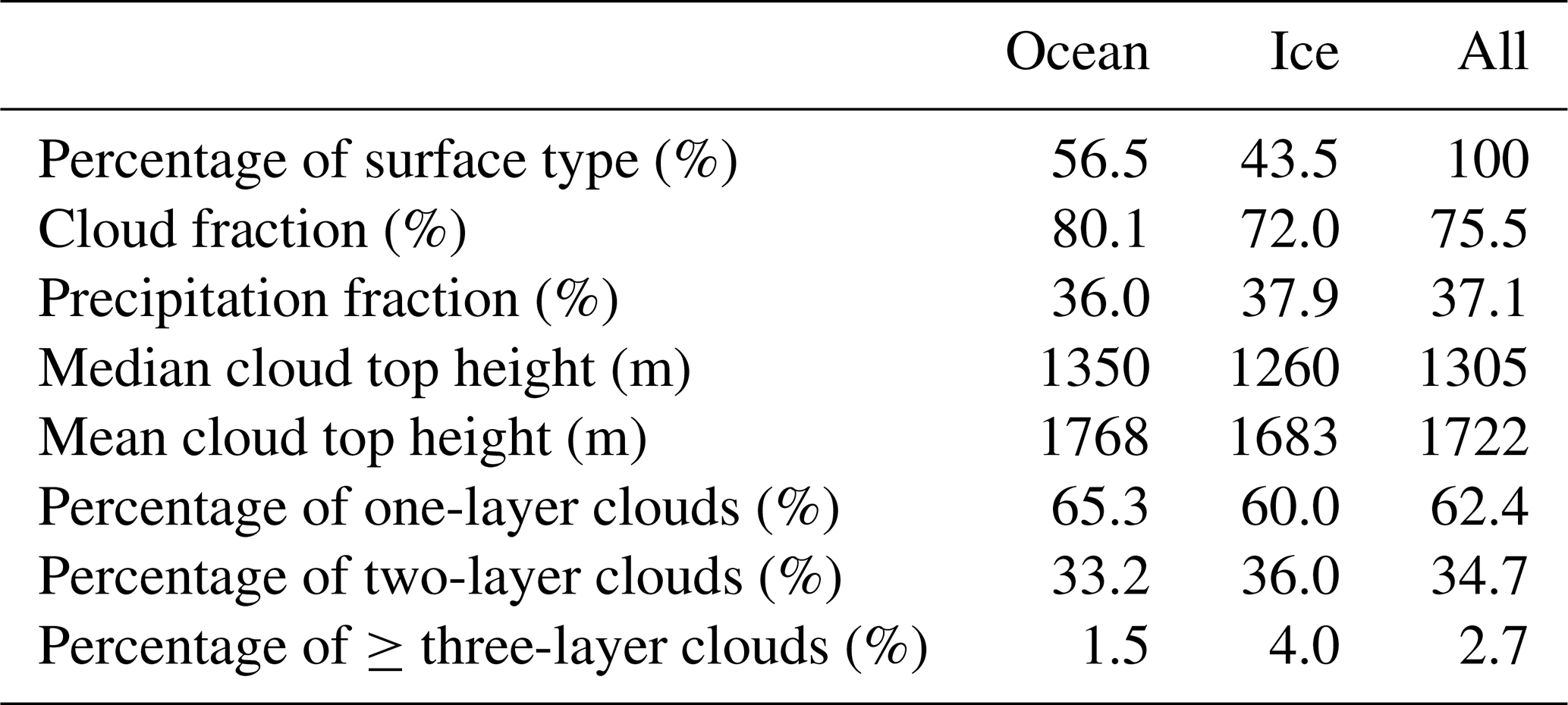
Table 5 Properties of clouds detected above ocean, sea ice, and both surface types.

A radar cloud mask is defined by considering profiles of Z_e. A profile is determined to be cloudy if a signal greater than Z_min (Fig. 1) reaches a vertical extent of more than 25 m, which roughly corresponds to two range gates for chirp table III (or one for chirps I and II; see Table 1). The cloud mask is then reduced to a one-dimensional vector along the flight track of ones and zeros describing clouds and clear sky, respectively. During the ACLOUD field campaign clouds occurred in 75 % of the flight time (Table 5), with 80 % over ocean and 72 % over sea ice. Figure 8 provides the cloud fraction vertically resolved in 100 m intervals. The highest values are present in the lowest 1000 m with about 25 % to 30 % over sea ice and 30 % over ocean (solid lines in Fig. 8). The cloud fraction is in general slightly higher over ocean than over sea ice at all heights. For measurements at higher levels (above 2850 m) the cloud fraction increases, which is most likely an artifact since measurements at higher levels were only taken when Polar 5 was forced to climb above clouds due to cloud tops exceeding the typical flight level 100 (corresponding to 3050 m).

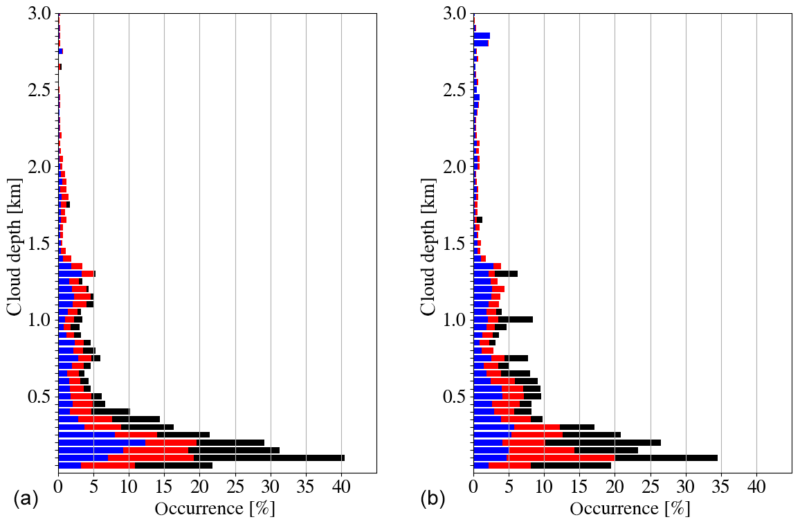
Figure 9 Cloud depth of single-layer and multilayer clouds. Blue describes the cloud depth distribution of all single-layer clouds, red describes depths of clouds with two layers, and black describes all cloud depths of clouds with three and more layers. For multilayer clouds the cloud depth of each layer is counted. The data are normalized such that all thickness bins of one type add up to 100 %. (a) Sea ice surface (>15 %); (b) ocean surface.

In order to characterize the cloud variability within the grid cell of a global climate model, cloud fraction is calculated for 20 min legs. With a typical flight speed of 80 m s⁻¹ this corresponds to roughly 100 km. The resulting distribution of cloud fraction for each height is shown in Fig. 8 in the form of box plots. Again, the highest variability with an interquartile range of 40 % or more occurs in the lowest 500 to 1000 m above ground level associated with low clouds and above 3 km due to the sampling. The radar signal is dominated by larger particles and therefore even few precipitating snow particles cause significant Z_e. Therefore, the averaged cloud fraction in the lowest altitudes amounting to roughly 30 % is likely due to snow precipitation. Interestingly, below 500 m the spread in cloud fraction decreases towards the ground, indicating the spatially rather constant occurrence of snow precipitation.

The radar cloud mask was used to derive information on cloud boundaries. This revealed that about 40 % of all clouds show cloud tops below 1000 m (Fig. 8), which are therefore likely to be missed by CloudSat. A total of 60 % of the cloud tops can be found below 1500 m. Throughout the observed 3000 m, the cloud tops over ocean are higher than the one over sea ice. When looking at the vertical structure of clouds 62 (35) % appear to be single-layer (two-layer) clouds (Table 5) and even three or more layers are identified about 3 % of the time. Looking at the thickness of these layers, not surprisingly, the multilayer clouds show the shortest vertical extent (median Δz=205 m) (Fig. 9). Over ice, there are almost no clouds that have vertical extents larger than 2000 m. Most clouds have thicknesses less than 1200 m, which is consistent with the most frequent cloud top heights (Fig. 8) and the frequent occurrence of precipitating clouds common for arctic mixed-phase stratiform clouds. As discussed in Sect. 4 the information on liquid water from the passive channels can be used over open ocean to determine the LWP. In this way, together with AMALi and radiation measurements, detailed insights into mixed-phase clouds will be gained.

In the beginning of the ACLOUD campaign a cold air outbreak could be observed, which showed the classical behavior of a thickening boundary layer with higher cloud top heights when transitioning from the sea ice to the open ocean. During the Aerosol-Cloud Coupling And Climate Interactions in the Arctic (ACCACIA) campaign Young et al. (2016) investigated the microphysical structure of clouds during such a cold air outbreak and found the largest number of concentrations of liquid droplets over sea ice decreasing towards the ocean while ice characteristics did not change significantly. In a first statistical attempt all profiles observed during ACLOUD were separated into ocean and sea ice surface conditions using the AMSR2 sea ice concentration and a threshold of 15 %. The number of measurements above sea ice and broken sea ice is higher than the number of measurements over open ocean (Fig. 8). Figure 8 additionally shows fewer clouds above sea ice, which most frequently occur below 800 m.

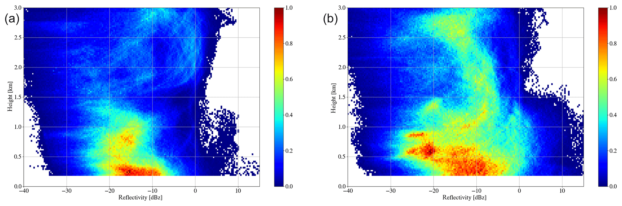
Figure 10 Contour frequency by altitude diagrams (CFADs) of sea ice (a) and ocean (b). The frequency is normalized by the highest number within the CFADs for each case, respectively. A sea ice fraction of >15 % is used (AMSR2).

After analyzing the macrophysical properties, constant frequency by altitude diagrams (CFADs; Yuter and Houze, 2002), which provide the frequency of occurrence of Z_e over the vertical profile, will now be considered. Figure 10 clearly shows the much lower vertical extent of clouds over sea ice. The highest frequency for Z_e occurs below 400 m between −20 and −10 dBz, indicating more frequent but rather low amounts of precipitation. A second cluster with a lower amount can be found between 500 and 1000 m with Z_e values between −20 and −15 dBz. Some higher reflectivities around 0 dBz can be between 2 and 3 km. In contrast measurements over open ocean show a higher concentration of reflectivities in the lowest levels between −15 and −8 dBz up to 500 m and a secondary peak of cloud clustering at −25 and −20 dBz between 500 and 900 m. This second peak that is not visible over sea ice corresponds to the elevated Arctic boundary layer height and the cloud forming there (Chechin and Lüpkes, 2019). A band spanning from around −10 dBz in 1 km to −18 dBz at 3 km belongs to the vertical-extending clouds over ocean. In general radar reflectivities are rather low with only a few measurements over ocean showing reflectivities higher than 0 dBz and almost none over ice. This emphasizes the need for a highly sensitive radar to observe Arctic low-level clouds.

6 Conclusions and outlook

The MiRAC is a novel airborne, active and passive microwave remote sensing instrument package with a 94 GHz FMCW radar and radiometers between 89 and 340 GHz. The instrument has been tailored to be fit into the Polar 5 aircraft and successfully participated in the ACLOUD campaign (Wendisch et al., 2018). A procedure to filter radar side lobes and to provide geo-referenced data to the community has been developed. The preliminary data analysis from ACLOUD clearly demonstrates the capabilities of MiRAC, especially for the study of low-level, mixed-phase Arctic clouds.

Deriving cloud microphysical properties from MiRAC and especially in synergy with other instruments, e.g., the AMALi lidar, operated on the Polar 5 will be the next step. As illustrated the passive channels are highly sensitive to sea ice, allowing us to determine the occurrence of sea ice with high spatial resolution. This, however, limits the possibility to retrieve cloud liquid water to open ocean. Exploring the information from the high-frequency channels in particular is of special interest in light of the upcoming MetOp-SG Ice Cloud Imager.

The Doppler spectra acquired by the MiRAC radar are difficult to interpret due to the influence of the aircraft motion on the Doppler shifts. Attempts to correct this are ongoing. Furthermore, information about multimode behavior in the spectra can also be used to better interpret the microphysics, especially for those flights where in situ measurements from the Polar 6 were performed.

During March–April 2019 MiRAC was part of the installation on Polar 5 in the Joint Aircraft campaign observing FLUXes of energy and momentum in the cloudy boundary layer over polar sea ice and ocean (AFLUX) flying out of Longyearbyen on Svalbard. In September 2019 the Multidisciplinary drifting Observatory for the Study of Arctic Climate (MOSAiC) campaign (http://www.mosaic-expedition.org, last access: 16 September 2019) will start. MiRAC-P will be operated in up-looking geometry on board the research vessel Polarstern to infer moisture profiles in the central Arctic. In March–April and August–September 2020 flights with MiRAC-A and a downward-looking Humidity And Temperature PROfiler (HATPRO; Rose et al., 2005) on board the Polar 5 aircraft will be performed again from Svalbard to further infer cloud characteristics in different seasons.

Appendix A: Coordinate transformation

First the mathematical basis of the coordinate transformation and the application to the experiment geometry followed by explicit coordinate transforms between the different reference frames discussed in Sect. 3 is provided.

A1 Mathematical basis

For the transition from one reference frame X_i to another X_j a mathematical operator T_ij called transform is introduced. It acts upon a position vector r⁽ⁱ⁾ in X_i coordinates and returns its coordinates r^(j) in X_j:

$$\begin{array}{}\text{(A1)}& {\mathit{r}}^{\left(j\right)}=T_{ij}\left({\mathit{r}}^{\left(i\right)}\right).\end{array}$$

The vector is first rotated, then shifted:

$$\begin{array}{}\text{(A2)}& T_{ij}\left({\mathit{r}}^{\left(i\right)}\right)={\mathbf{R}}_{ij}\cdot {\mathit{r}}^{\left(i\right)}+{\mathit{S}}_{ij},\end{array}$$

where R_ij is a matrix expressing the rotation of X_i relative to X_j, S_ij is the position of X_i in coordinates of X_j, and ⋅ is the matrix product.

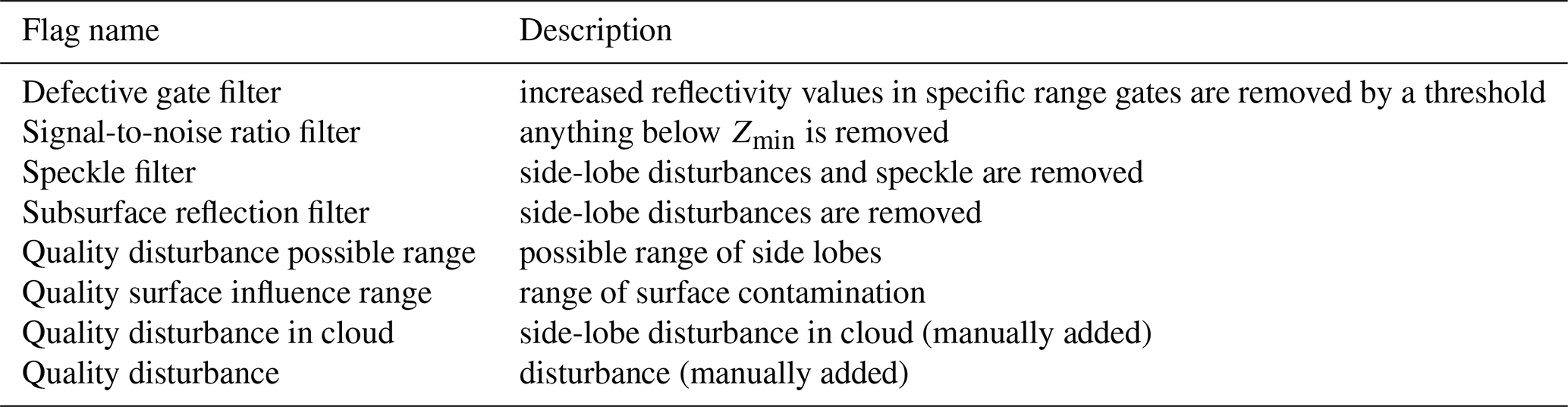
Table A1 Filter names and quality control of data in PANGAEA files (Kliesch and Mech, 2019), description to variable “Ze flag” rows 1 to 4 is already applied to get from “Ze unfiltered” to “Ze” and rows 5 to 8 help for analyzing the data.

The inverse of the transform is obtained by solving Eq. (A2) for r⁽ⁱ⁾:

$$\begin{array}{}\text{(A3)}& T_{ji}\left({\mathit{r}}^{\left(j\right)}\right)={\mathbf{R}}_{ij}^{-\mathrm{1}}\cdot {\mathit{r}}^{\left(j\right)}-{\mathbf{R}}_{ij}^{-\mathrm{1}}\cdot {\mathit{S}}_{ij},\end{array}$$

with ⁻¹ being the matrix inversion operator (the inverse of a rotation matrix can be easily obtained by transposition). Equation (A3) has the same form as Eq. (A2), with rotation ${\mathbf{R}}_{ji}={\mathbf{R}}_{ij}^{-\mathrm{1}}$ and shift ${\mathit{S}}_{ji}=\left(-{\mathbf{R}}_{ij}^{-\mathrm{1}}\cdot {\mathit{S}}_{ij}\right)$.

The composition of two transforms T_ij (from X_i to X_j) and T_jk (from X_j further to X_k) yields the direct transform from X_i to X_k. It is obtained by applying T_jk to the result of T_ij:

$$\begin{array}{}\text{(A4)}& T_{ik}\left({\mathit{r}}^{\left(i\right)}\right)=\left({\mathbf{R}}_{jk}\cdot {\mathbf{R}}_{ij}\right)\cdot {\mathit{r}}^{\left(i\right)}+\left({\mathbf{R}}_{jk}\cdot {\mathit{S}}_{ij}+{\mathit{S}}_{jk}\right),\end{array}$$

where ${\mathbf{R}}_{ik}=\left({\mathbf{R}}_{jk}\cdot {\mathbf{R}}_{ij}\right)$ and ${\mathit{S}}_{ik}=\left({\mathbf{R}}_{jk}\cdot {\mathit{S}}_{ij}+{\mathit{S}}_{jk}\right)$ can be identified, respectively, as the rotation and shift of the composed transform.

A2 Application to the experiment geometry

Once the three base transforms connecting the four reference frames X_s, X_p, X_c, and X_g are established, the coordinates of the measurement targets can be transformed from X_s to X_g by applying the transform

$$\begin{array}{}\text{(A5)}& T_{\mathrm{sg}}=T_{\mathrm{cg}}\circ T_{\mathrm{pc}}\circ T_{\mathrm{sp}}\end{array}$$

to the position vector r^(s) of the measurement (since measurements are only performed along the y^(s) axis, ${\mathit{r}}^{\left(\mathrm{s}\right)}=r\cdot {\mathit{e}}_y$) the transforms are obtained in principle.

The transform T_sp from X_s to X_p is independent of time. It is described by the location of the payload sensor relative to the position sensor and by the orientation of the payload sensor relative to the sensor attitude. These relations are known from surveys before the campaign.

The time-dependent transform T_pc from X_p to X_c is purely rotational as the two reference frames are co-located. It is described by the three principal rotation angles of the platform (Fig. 6). To reach X_p from X_c, the coordinate system is first rotated by the (true) heading η (distance to north) about the z axis in a mathematically negative sense. Then, a rotation about the x axis by the pitch angle ϵ is applied (elevation of the nose). Finally, the system is rotated about the y axis by the roll angle ρ. These three angles are recorded by the attitude sensor, which in practice is an inertial navigation system (INS) on board the aircraft.

The transform T_cg from X_c to X_g (λ, ϕ, h) is time dependent, too. It is done with knowledge of the platform position relative to the planet, which is recorded by the position sensor (e.g., by use of a radio navigation satellite service such as GPS). Since X_c is aligned with the local east, north, and zenith, both shift and rotation of T_cg are determined by the platform position.

A3 From X_s to X_p

The shift part of T_sp is the sensor position in X_s coordinates:

$$\begin{array}{}\text{(A6)}& {\mathit{S}}_{\mathrm{sp}}={\mathit{r}}_{\mathrm{s}}^{\left(\mathrm{p}\right)}.\end{array}$$

As the x^(s) and z^(s) axes are undefined, the rotation is sufficiently described by two angles: The azimuth angle ${\mathit{\alpha }}_{\mathrm{s}}^{\left(\mathrm{p}\right)}$ measures how far the payload sensor's line of sight is rotated about the platform's z^(p) axis away from the forward direction (y^(p) axis); it is measured in mathematically negative sense (forward–right–backward–left). The view angle ${\mathit{\beta }}_{\mathrm{s}}^{\left(\mathrm{p}\right)}$ is the distance to the negative z^(p) axis (i.e., zero if looking downward with respect to the platform reference frame). The rotational part of T_sp is the successive application of these two rotations:

$$\begin{array}{}\text{(A7)}& {\mathbf{R}}_{\mathrm{sp}}={\mathbf{R}}_{\mathrm{sp},\mathit{\alpha }}\cdot {\mathbf{R}}_{\mathrm{sp},\mathit{\beta }},\end{array}$$

with

$$\begin{array}{}\text{(A8)}& {\displaystyle }& {\displaystyle }{\mathbf{R}}_{\mathrm{sp},\mathit{\alpha }}=\left(\begin{array}{ccc}\cos {\mathit{\alpha }}_{\mathrm{s}}^{\left(\mathrm{p}\right)}& \sin {\mathit{\alpha }}_{\mathrm{s}}^{\left(\mathrm{p}\right)}& \mathrm{0}\\ -\sin {\mathit{\alpha }}_{\mathrm{s}}^{\left(\mathrm{p}\right)}& \cos {\mathit{\alpha }}_{\mathrm{s}}^{\left(\mathrm{p}\right)}& \mathrm{0}\\ \mathrm{0}& \mathrm{0}& \mathrm{1}\end{array}\right)\text{(A9)}& {\displaystyle }& {\displaystyle }{\mathbf{R}}_{\mathrm{sp},\mathit{\beta }}=\left(\begin{array}{ccc}\mathrm{1}& \mathrm{0}& \mathrm{0}\\ \mathrm{0}& \sin {\mathit{\beta }}_{\mathrm{s}}^{\left(\mathrm{p}\right)}& \cos {\mathit{\beta }}_{\mathrm{s}}^{\left(\mathrm{p}\right)}\\ \mathrm{0}& -\cos {\mathit{\beta }}_{\mathrm{s}}^{\left(\mathrm{p}\right)}& \sin {\mathit{\beta }}_{\mathrm{s}}^{\left(\mathrm{p}\right)}\end{array}\right).\end{array}$$

A4 From X_p to X_c

Since the origins of the two reference frames are identical, this transform is purely rotational. The platform attitude relative to X_c is described by the angles η, ϵ, and ρ (Sect. 3.2, the superscript ^(c) is omitted here). The transition from X_p to X_c is achieved by successively reversing these rotations:

$$\begin{array}{}\text{(A10)}& {\mathbf{R}}_{\mathrm{pc}}={\mathbf{R}}_{\mathrm{pc},\mathit{\eta }}\cdot {\mathbf{R}}_{\mathrm{pc},\mathit{ϵ}}\cdot {\mathbf{R}}_{\mathrm{pc},\mathit{\rho }},\end{array}$$

with

$$\begin{array}{}\text{(A11)}& {\displaystyle }& {\displaystyle }{\mathbf{R}}_{\mathrm{pc},\mathit{\eta }}=\left(\begin{array}{ccc}\cos \mathit{\eta }& \sin \mathit{\eta }& \mathrm{0}\\ -\sin \mathit{\eta }& \cos \mathit{\eta }& \mathrm{0}\\ \mathrm{0}& \mathrm{0}& \mathrm{1}\end{array}\right)\text{(A12)}& {\displaystyle }& {\displaystyle }{\mathbf{R}}_{\mathrm{sp},\mathit{ϵ}}=\left(\begin{array}{ccc}\mathrm{1}& \mathrm{0}& \mathrm{0}\\ \mathrm{0}& \cos \mathit{ϵ}& -\sin \mathit{ϵ}\\ \mathrm{0}& \sin \mathit{ϵ}& \cos \mathit{ϵ}\end{array}\right)\text{(A13)}& {\displaystyle }& {\displaystyle }{\mathbf{R}}_{\mathrm{sp},\mathit{\rho }}=\left(\begin{array}{ccc}\cos \mathit{\rho }& \mathrm{0}& \sin \mathit{\rho }\\ \mathrm{0}& \mathrm{1}& \mathrm{0}\\ -\sin \mathit{\rho }& \mathrm{0}& \cos \mathit{\rho }\end{array}\right).\end{array}$$

A5 From X_c to X_g

Here, the platform position is used. It is usually recorded in the spherical coordinates longitude λ_c, latitude ϕ_c, and altitude h_c above mean sea level (superscript ^(g) is omitted here). Note that, because the origins of X_c and X_p coincide, λ^(c)=λ^(p), ϕ^(c)=ϕ^(p), and h^(c)=h^(p). They sufficiently describe both the shift and the rotation of T_cg. The shift part of T_cg is the platform position within X_g:

$$\begin{array}{}\text{(A14)}& {\mathit{S}}_{\mathrm{cg}}=(x_{\mathrm{c}}^{\mathrm{g})},y_{\mathrm{c}}^{\left(\mathrm{g}\right)},z_{\mathrm{c}}^{\left(\mathrm{g}\right)}),\end{array}$$

where $(x_{\mathrm{c}}^{\left(\mathrm{g}\right)},y_{\mathrm{c}}^{\left(\mathrm{g}\right)},z_{\mathrm{c}}^{\left(\mathrm{g}\right)})$ is the Cartesian representation of $({\mathit{\lambda }}_{\mathrm{c}},{\mathit{\varphi }}_{\mathrm{c}},h_{\mathrm{c}})$. The rotation matrix is established by first accounting for the latitude, then for the longitude:

$$\begin{array}{}\text{(A15)}& {\mathbf{R}}_{\mathrm{cg}}={\mathbf{R}}_{\mathrm{cg},\mathit{\lambda }}\cdot {\mathbf{R}}_{\mathrm{cg},\mathit{\varphi }},\end{array}$$

with

$$\begin{array}{}\text{(A16)}& {\displaystyle }& {\displaystyle }{\mathbf{R}}_{\mathrm{cg},\mathit{\lambda }}=\left(\begin{array}{ccc}-\sin {\mathit{\lambda }}_c& \cos {\mathit{\lambda }}_c& \mathrm{0}\\ \cos {\mathit{\lambda }}_c& \sin {\mathit{\lambda }}_c& \mathrm{0}\\ \mathrm{0}& \mathrm{0}& \mathrm{1}\end{array}\right)\text{(A17)}& {\displaystyle }& {\displaystyle }{\mathbf{R}}_{\mathrm{cg},\mathit{\varphi }}=\left(\begin{array}{ccc}\mathrm{1}& \mathrm{0}& \mathrm{0}\\ \mathrm{0}& \sin {\mathit{\varphi }}_c& -\cos {\mathit{\varphi }}_c\\ \mathrm{0}& \cos {\mathit{\varphi }}_c& \sin {\mathit{\varphi }}_c\end{array}\right).\end{array}$$

A6 From X_s to X_g

A transform directly from X_s to X_g can be obtained by use of the composition formula in Eq. (A4):

$$\begin{array}{}\text{(A18)}& T_{\mathrm{sg}}=T_{\mathrm{cg}}\circ T_{\mathrm{pc}}\circ T_{\mathrm{sp}}.\end{array}$$

This is conveniently done by a computing machine. The explicit form of T_sg is not derived.

In order to obtain the target coordinates in spherical representation, the position vector in X_g is eventually reconverted to spherical coordinates after application of the transform.