Use of spectral cloud emissivities and their related uncertainties to infer ice cloud boundaries: methodology and assessment using CALIPSO cloud products

Satellite-imager-based operational cloud property retrievals generally assume that a cloudy pixel can be treated as being plane-parallel with horizontally homogeneous properties. This assumption can lead to high uncertainties in cloud heights, particularly for the case of optically thin, but geometrically thick, clouds composed of ice particles. This study demonstrates that ice cloud emissivity uncertainties can be used to provide a reasonable range of ice cloud layer boundaries, i.e., the minimum to maximum heights. Here ice cloud emissivity uncertainties are obtained for three IR channels centered at 11, 12, and 13.3 µm. The range of cloud emissivities is used to infer a range of ice cloud temperature and heights, rather than a single value per pixel as provided by operational cloud retrievals. Our methodology is tested using MODIS observations over the western North Pacific Ocean during August 2015. We estimate minimum–maximum heights for three cloud regimes, i.e., single-layered optically thin ice clouds, single-layered optically thick ice clouds, and multilayered clouds. Our results are assessed through comparison with CALIOP version 4 cloud products for a total of 11873 pixels. The cloud boundary heights for single-layered optically thin clouds show good agreement with those from CALIOP; biases for maximum (minimum) heights versus the cloud-top (base) heights of CALIOP are 0.13 km (−1.01 km). For optically thick and multilayered clouds, the biases of the estimated cloud heights from the cloud top or cloud base become larger (0.30/−1.71 km, 1.41/−4.64 km). The vertically resolved boundaries for ice clouds can contribute new information for data assimilation efforts for weather prediction and radiation budget studies. Our method is applicable to measurements provided by most geostationary weather satellites including the GK-2A advanced multichannel infrared imager.

1 Introduction

Satellite sensors provide data daily that are essential for determining global cloud properties, including cloud height–pressure–temperature, thermodynamic phase (ice or liquid water), cloud optical thickness, and effective particle size. These variables are essential for understanding the net radiation of the Earth and the impact of clouds (L'Ecuyer et al., 2019). In particular, cloud heights at the top and base levels are necessary to determine upwelling and downwelling infrared (IR) radiation (Slingo and Slingo, 1988; Baker, 1997; Harrop and Hartmann; 2012). Additionally, cloud heights are used to derive atmospheric motion vectors that are important for most global data-assimilation systems (Bouttier and Kelly, 2001), affecting the accuracy of the global model forecast (Lee and Song, 2018). However, in most operational retrievals of cloud properties, only a single cloud height is inferred for a given pixel, or field of view. The goal of this study is to develop an algorithm to infer cloud height boundaries for semitransparent ice clouds using only IR measurements for its applicability of global data regardless of solar illumination. Where this study could provide the most benefit is for the case where an ice cloud is geometrically thick but optically thin.

Although our approach will be applied to geostationary satellites in future work, the algorithm is developed for the Moderate Resolution Imaging Spectroradiometer (MODIS) sensor for two reasons: (1) our resulting cloud temperatures can be compared to those from the Cloud-Aerosol Lidar and Infrared Pathfinder Satellite Observation Cloud-Aerosol Lidar with Orthogonal Polarization (CALIPSO CALIOP) active lidar version 4 products for verification and (2) further comparison can be made to the MODIS Collection 6 cloud products. The approach adopted in our study for the inference of ice cloud height has a basis in the work of Inoue (1985), who developed this approach using only the split-window channels on the Advanced Very High Resolution Radiometer (AVHRR). The goal of the Inoue (1985) approach was to improve the inference of cloud temperatures for semitransparent ice clouds. Heidinger and Pavolonis (2009) further improved this approach and generated a 25-year climatology of ice cloud properties from AVHRR analysis.

For satellite-based cloud height retrievals based on passive IR measurements, the radiative emission level is regarded as the cloud top. When the emissivity is 1, the cloud is emitting as a blackbody and the cloud top is at, or close to, the actual cloud's upper boundary. As the emissivity decreases, the cloud top inferred from IR measurements will be lower than the actual cloud-top level. This is demonstrated in Holz et al. (2006), who compared the cloud tops from aircraft Scanning High-Resolution Interferometer Sounder (S-HIS) measurements to those from coincident measurements from the Cloud Physics Lidar (CPL). They found that the best match between the cloud tops based on the passive S-HIS measurements and the CPL occurs when the integrated cloud optical thickness is approximately 1. This implies that the differences of cloud-top heights by IR measurements from those by CALIOP are expected since the IR method reports the height where the integrated cloud optical thickness, beginning at cloud top and moving downwards into the cloud, is approximately 1 while CALIOP reports the actual cloud top to be where the first particles are encountered.

With regard to geometric differences of IR cloud tops from the actual cloud tops, optically thin but geometrically thick clouds show the largest bias since the level at which the integrated optical thickness reaches 1 is much lower than the height at which the first ice particles occur. In a review of 10 different satellite retrieval methods for cloud-top heights by IR measurements (Hamann et al., 2014), the heights inferred for optically thin clouds are generally below the cloud's mid-level height. When lower-level clouds are present below the cirrus in a vertical column, the inferred cloud height can be between the cloud layers, depending on the optical thickness of the uppermost layer.

There is a retrieval approach to infer optically thin cloud-top pressure that uses multiple IR absorption bands within the 15 µm CO₂ band (e.g., Menzel et al., 2008; Baum et al., 2012), called the CO₂ slicing method. These 15 µm CO₂ band channels are available on the Terra–Aqua MODIS imagers, the HIRS sounders, and with any hyperspectral IR sounder (IASI, CrIS, AIRS). MODIS is the only imager where multiple 15 µm CO₂ channels are available. Zhang and Menzel (2002) showed improvement of the retrieval of ice cloud height when they take into account spectral cloud emissivity that has some sensitivity to the cloud microphysics. As the goal of our work is to develop a reliable method for inferring ice cloud height from geostationary data, we are limiting this study to the use of the relevant IR channels, i.e., measurements at 11, 12, and 13.3 µm.

To complement the use of IR window channels, the addition of a single IR absorption channel, such as one within the broad 15 µm CO₂ band, has been shown to improve the inference of cirrus cloud temperature (Heidinger et al., 2010). Their study shows how adding a single IR absorption channel at 13.3 µm to the IR 11 and 12 µm window channels decreases the solution space in an optimal estimation retrieval approach and leads to closer comparisons in cloud height–temperature with CALIPSO CALIOP cloud products.

Rather than inferring a single ice cloud temperature in each pixel, we infer a range of ice cloud temperatures (minimum to maximum temperature per ice cloud pixel) that correspond to uncertainties in the cloud spectral emissivity. We note that the spectral cloud emissivity, which can be obtained using measurements at 11, 12, and 13.3 µm, has some dependence on the ice cloud microphysics. The emissivities are subsequently used to estimate ranges of cloud height, which are found by converting the estimated cloud temperature ranges using a simple linear interpolation of the Numerical Weather Prediction (NWP) model profiles. Cloud boundary results are presented for three cloud categories, i.e., single-layered optically thin ice clouds, single-layered optically thick ice clouds, and multilayered clouds, and these results are assessed with measurements from a month of collocated CALIOP version 4 data. The focus area for the data analysis and resulting analyses is the western North Pacific Ocean for the month of August 2015.

The paper is organized as follows. Section 2 describes the data used in this study. Section 3 presents the methodology and the generation of the relevant look-up tables (LUTs) for the radiances and brightness temperatures used in our analyses. Section 4 provides results for the western North Pacific Ocean during August 2015 and comparisons with CALIOP. Section 5 discusses the results and Sect. 6 summarizes this paper.

2 Data

2.1 Study domain

The study domain is the western North Pacific Ocean (0–30^∘ N, 120–170^∘ E) during August each year from 2013 to 2015. Two of these months (August 2013 and August 2014) are used for generating the LUTs, while the month of August in 2015 is used for testing and validating the current algorithm. The reason for restriction of the study domain is to obtain a clear relationship between radiances–brightness temperatures and spectral cloud emissivity. In the western North Pacific Ocean, the ice clouds can be generated from diverse meteorological conditions including frequent typhoons.

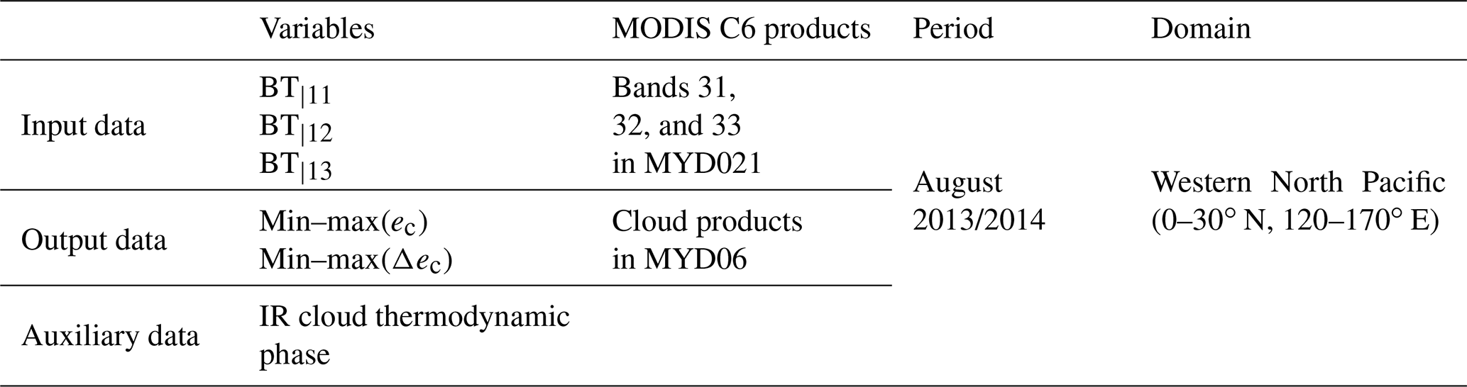
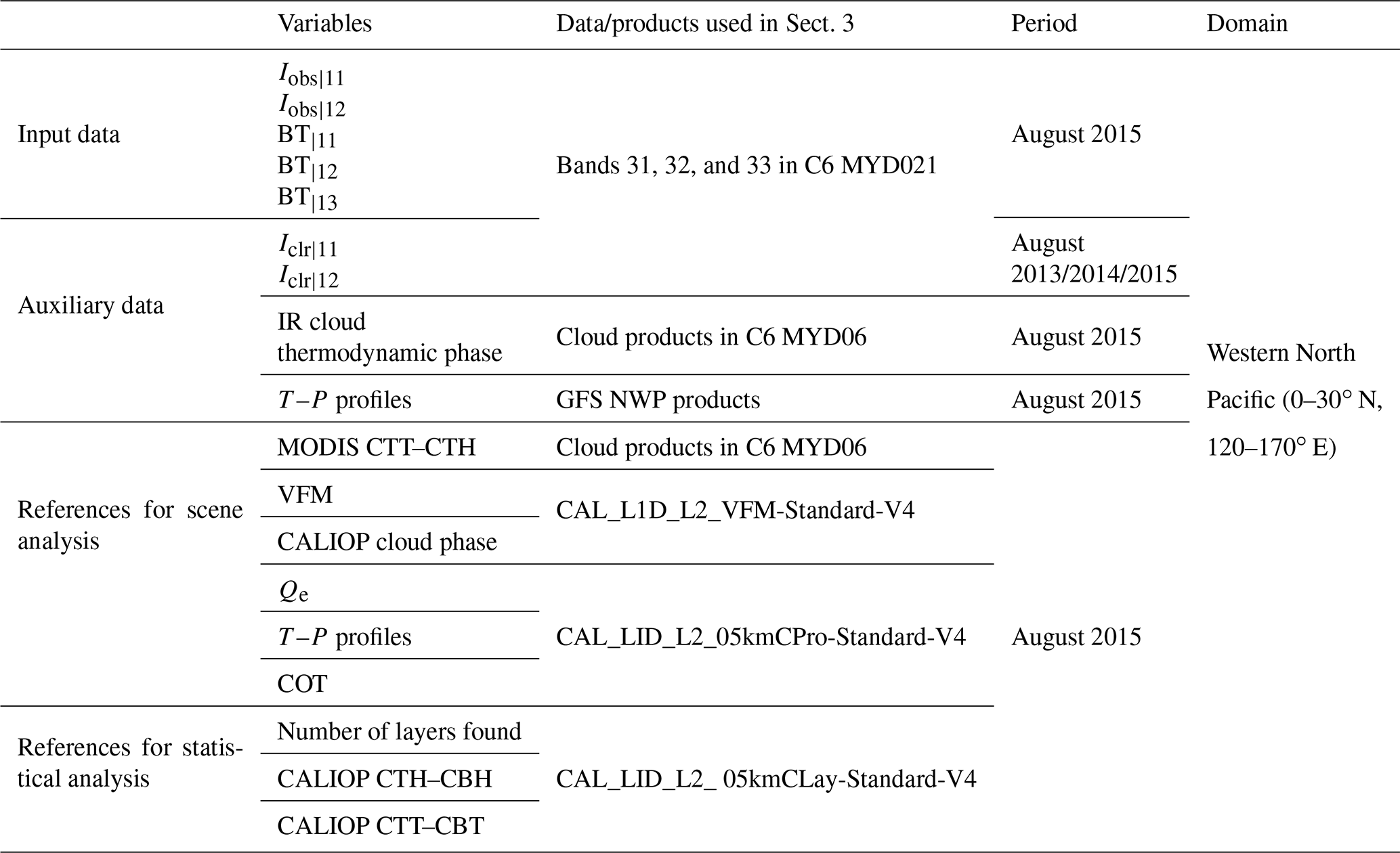
Table 1 The detailed information used to generate empirical look-up tables (LUTs) of min–max(e_c) and min–max(Δe_c). MODIS bands 31, 32, and 33 have spectral wavelengths ranges of 10.78–11.28, 11.77–12.27, and 13.185–13.485 µm, respectively.

2.2 Aqua Moderate Resolution Imaging Spectroradiometer (MODIS)

The MODIS is a 36-channel whisk-broom scanning radiometer on the NASA Earth Observing System Terra and Aqua platforms. The Aqua platform is in a daytime ascending orbit at 13:30 LST. The MODIS sensor has four focal planes that cover the spectral range 0.42–14.24 µm. The longwave bands are calibrated with an onboard blackbody. Table 1 shows the Aqua MODIS products used in this study; these products include the Collection 6 1 km Level-1b radiance data (MYD021KM), geolocation data (MYD03), and cloud properties at 1 km resolution (MYD06). In this study, the radiances and brightness temperatures at 11, 12, and 13.3 µm (channels 31, 32, and 33, respectively) are taken from the C6 MYD021KM data. Latitude–longitude information for each granule is from C6 MYD03. The C6 MYD06 product provides cloud emissivity values in the IR window (8.5, 11, and 12 µm) and also cloud-top height (CTH), all at 1 km spatial resolution; these parameters were not included in earlier collections (Menzel et al., 2008; Baum et al., 2012). The cloud emissivities at 11 and 12 µm are used in this study.

2.3 CALIPSO CALIOP

The CALIPSO satellite platform carries several instruments, among which is a near-nadir-viewing lidar called CALIOP (Winker et al., 2007, 2009). Originally, CALIPSO flew in formation with NASA's Earth Observing System Aqua platform since 2006 and was part of the A-Train suite of sensors. At the time of this writing, it is no longer part of the A-Train but flies in formation with CloudSat in a lower orbit. CALIOP takes data at 532 and 1064 nm. The CALIOP 532 nm channel also measures the linear polarization state of the lidar returns. The depolarization ratio contains information about aerosol and cloud properties. This study uses CALIPSO version 4 products that were released in November 2016. With the updated radiometric calibration at 532 and 1064 nm (Getzewich et al., 2018; Vaughan et al., 2019), cloud products such as cloud–aerosol discrimination and extinction coefficients show significant improvement relative to previous versions (Young et al., 2018; Liu et al., 2019). CALIPSO products are used to validate our retrievals, including CAL_L1D_L2_ VFM-Standard-V4, which provides cloud vertical features; CAL_LID_L2_05kmCPro-Standard-V4 and CAL_LID_L2_05kmCLay-Standard-V4, which provide cloud-top and cloud-base temperature (height); extinction coefficients; and temperature profiles (Table 1).

2.4 Numerical weather model product

The Global Forecast System (GFS) model is produced by the National Centers for Environmental Prediction (NCEP) of the National Oceanic and Atmospheric Administration (NOAA) (Moorthi et al., 2001). GFS provides global NWP model outputs at 0.5^∘ resolution at 3 h forecast intervals every 6 h that are available online (https://www.ncdc.noaa.gov/data-access/model-data/model-datasets/global-forcast-system-gfs, last access: 31 March 2019). We use two variables from the NWP products, temperature profiles, and geopotential heights, with cloud heights provided for 26 isobaric layers that are related to cloud temperatures. These data are used for the conversion of cloud temperatures to cloud heights. The NWP fields are remapped to the resolution of satellite imagery by linear interpolation. We use the NWP products that are closest in time to the satellite observations.

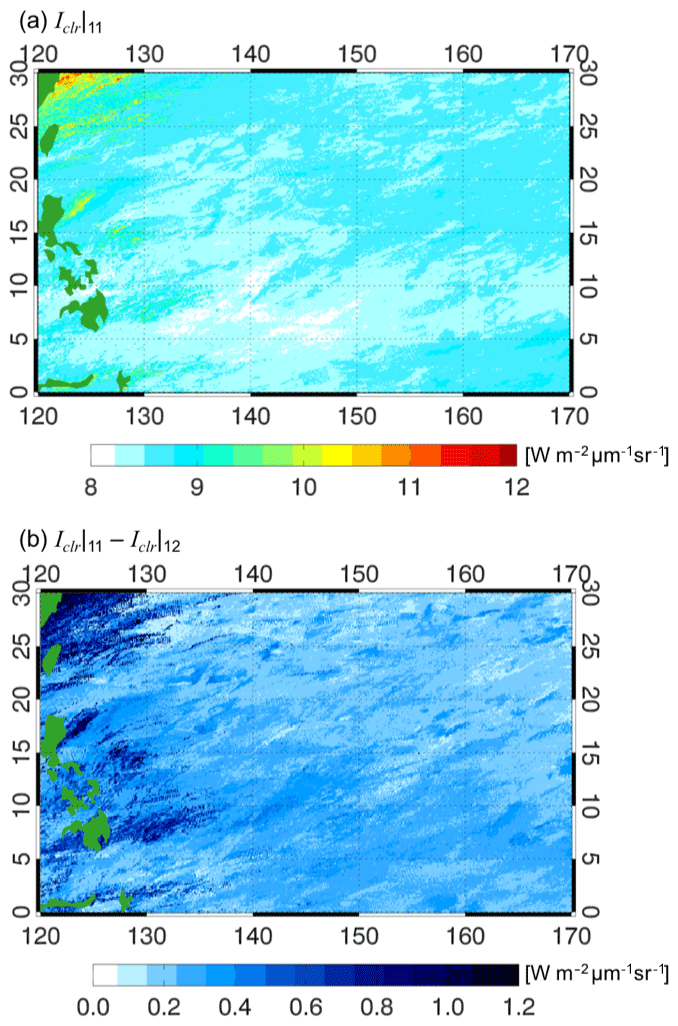
Figure 1 The estimated clear-sky radiance map at $\mathrm{0.1}{}^{\circ }\times \mathrm{0.1}{}^{\circ }$ resolution for (a) 11 µm (I_clr|11) and (b) differences of 11 µm from 12 µm ($I_{\mathrm{clr}|\mathrm{11}}-I_{\mathrm{clr}|\mathrm{12}}$) in units of W m⁻² µm⁻¹ sr⁻¹. I_clr|11 and I_clr|12 are the maximum values among MODIS C6 radiances for August in 3 three years (2013–2015) in each $\mathrm{0.1}{}^{\circ }\times \mathrm{0.1}{}^{\circ }$ grid box. Green-shaded contours over the map show land, which is generally from the Philippines.

2.5 Clear-sky maps generated from MODIS

The MODIS pixels identified as being clear sky are used to generate a gridded clear-sky map, which is another ancillary product required for our method. To simplify the generation of this map, the MODIS data with 1 km resolution are converted to 5 km resolution. Monthly composites of clear-sky radiances (I_clr) at $\mathrm{0.1}{}^{\circ }\times \mathrm{0.1}{}^{\circ }$ resolution are generated by choosing the maximum value among radiances for August in 3 years (2013–2015) in each $\mathrm{0.1}{}^{\circ }\times \mathrm{0.1}{}^{\circ }$ grid box. To confirm the availability of the generated I_clr, we present the spatial distribution of I_clr at 11 µm (I_clr|11, Fig. 1a), from 8 to 11 W m⁻² µm⁻¹ sr⁻¹. The largest I_clr|11 values are shown over the northwestern region of the domain, whereas the smallest I_clr|11 values are shown over the southeastern region of the domain. The pattern of I_clr|11 is similar to the spatial distribution of the monthly average of sea surface temperature in 2015 (https://bobtisdale.wordpress.com/2015/09/08/august-2015-sea-surface-temperature-sst-anomaly-update/, last access: 31 March 2019). Also, we show the spatial distribution of spatial distribution of differences of I_clr|11 from I_clr|12 in Fig. 1a, examining the reliability of the generated I_clr|12. Note that the differences of I_clr|11 and I_clr|12 are positive over the domain because water vapor absorption is stronger at 12 µm than at 11 µm. Large differences are shown in the western region, near the Philippines (green-colored contours in Fig. 1).

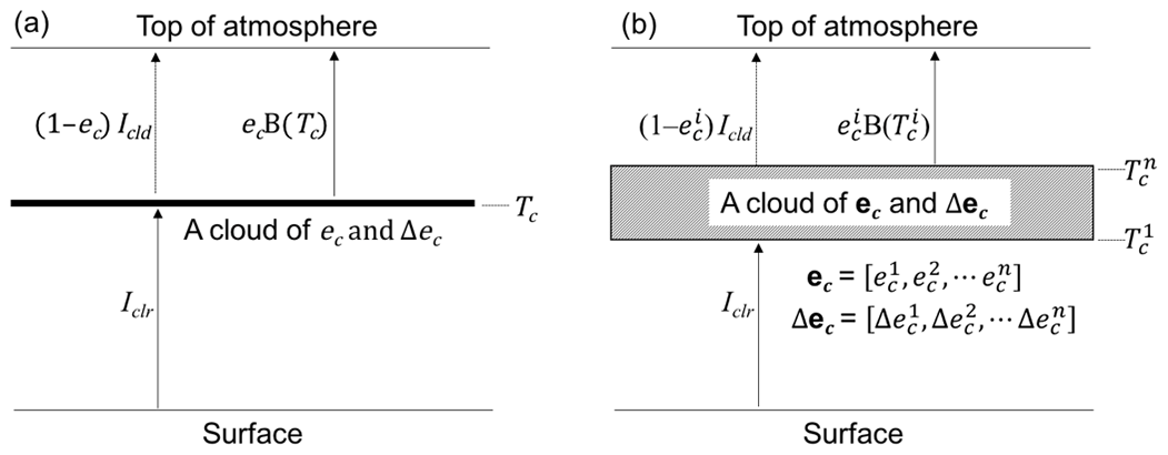
Figure 2 The conceptual model for (a) a plane-parallel homogeneous cloud layer with no scattering, characterized by cloud emissivity (e_c) and cloud emissivity differences between two infrared channels (Δe_c) at the cloud temperature (T_c) and (b) a number of plane-parallel homogeneous cloud layers (the stripes box) with a possible range of e_c and Δe_c such as $e_{\mathrm{c}}=[e_{\mathrm{c}}^{\mathrm{1}}{e}_{\mathrm{c}}^{\mathrm{2}}\mathrm{\dots },e_{\mathrm{c}}^n$] and $\mathrm{\Delta }{e}_{\mathrm{c}}=[\mathrm{\Delta }{e}_{\mathrm{c}}^{\mathrm{1}}\mathrm{\Delta }{e}_{\mathrm{c}}^{\mathrm{2}}\mathrm{\dots },\mathrm{\Delta }{e}_{\mathrm{c}}^n$] corresponding to a possible range of cloud temperature, $T_{\mathrm{c}}=[T_{\mathrm{c}}^{\mathrm{1}}{T}_{\mathrm{c}}^{\mathrm{2}}\mathrm{\dots },T_{\mathrm{c}}^n$], where I_clr and B are the clear-sky radiance and the Planck's function, respectively. Arrows represent upwelling radiances.

3 Methodology

3.1 Cloud retrieval algorithm

The basis for the retrieval algorithm is provided in Inoue (1985). Figure 2a shows the plane-parallel homogeneous cloud model with no scattering. The ice cloud layer at a given height has a corresponding ice cloud temperature (T_c) and an associated cloud emissivity (e_c). The observed upwelling radiance (I_obs) at the cloud top is composed of two terms: the first depending on the upwelling clear-sky radiance (I_clr) at the cloud base and the other depending on the radiance (B(T_c)) computed for a cloud emitting as a blackbody:

$$\begin{array}{}\text{(1)}& I_{\mathrm{obs}}=\left(\mathrm{1}-e_{\mathrm{c}}\right)I_{\mathrm{clr}}+e_{\mathrm{c}}B\left(T_{\mathrm{c}}\right),\end{array}$$

where B(T_c) is the Planck emission for a cloud computed at T_c (Liou, 2002). All terms in Eq. (1) are wavelength dependent except for the T_c. I_obs is determined from the satellite measurements, and I_clr can be found from clear-sky conditions in the imagery or computed by a radiative transfer model given a set of atmospheric profiles of temperature, humidity, and trace gases. However, e_c and T_c are unknown.

Equation (1) can be rearranged to solve for the emissivity:

$$\begin{array}{}\text{(2)}& e_{\mathrm{c}}=(I_{\mathrm{obs}}-I_{\mathrm{clr}})/(B\left(T_{\mathrm{c}}\right)-I_{\mathrm{clr}}).\end{array}$$

One can relate two channels by taking a ratio of the radiances, similar to that of the CO₂ slicing method (e.g., Menzel et al., 2008), and assuming that the emissivity between two channels spaced closely in wavelength are the same. However, Zhang and Menzel (2002) showed improvement of the retrieval of ice cloud pressure by accounting for differences in the spectral cloud emissivity.

Inoue (1985) discusses the range of uncertainties in both T_c and e_c and further suggests that use of multiple IR channels can reduce the uncertainties. To relate the effective emissivity between two channels, Inoue uses the relation of the cirrus emissivity to the optical thickness. The e_c is a function of the absorption coefficient (κ) and the cloud thickness (z),

$$\begin{array}{}\text{(3)}& e_{\mathrm{c}}=\mathrm{1}-{\exp }^{-\mathit{\kappa }z/\mathit{\mu }}.\end{array}$$

The term μ in Eq. (3) is a cosine of the viewing zenith angle; the quantity κz is called the optical thickness and is also wavelength dependent. Given a value for e_c, the T_c can be obtained by Eq. (2). The estimate of e_c from an IR measurement will have inherent uncertainties due to the diversity of ice particle size distributions (i.e., cloud microphysics), sensor calibration, and in-cloud vertical inhomogeneity.

Another way to constrain these uncertainties is by using multiple IR channel measurements, specifically the spectral emissivity differences between two IR window channels (Δe_c). We can express the Δe_c between two IR channels by

$$\begin{array}{}\text{(4)}& \mathrm{\Delta }{e}_{\mathrm{c}}={\exp }^{-\frac{{\mathit{\kappa }}^{\prime }z}{\mathit{\mu }}}-{\exp }^{-\frac{\mathit{\kappa }z}{\mathit{\mu }}}.\end{array}$$

In Eq. (4), κ^′ is the absorption coefficient at “another” IR window channel. That is, the Δe_c is determined by ($\mathit{\kappa }-{\mathit{\kappa }}^{\prime })/z$, which depends on the cloud particle size and cloud thickness (Kikuchi et al., 2006). Many studies have adopted this, or a similar, approach to apply the representative relations of spectral cloud emissivity relying on cloud types to retrieve the T_c (e.g., Inoue, 1985; Parol et al., 1991; Giraud et al., 1997; Cooper et al., 2003; Heidinger and Pavolonis, 2009).

For the case of two IR channels, Inoue (1985) formulated the retrieval of the cirrus cloud temperature and effective emissivity by setting up three equations with three unknowns (specifically referring to Inoue's equations 5, 6, and 7): two equations are the same as Eq. (2) at 11 and 12 µm in this paper, and the last equation is as follows.

$$\begin{array}{}\text{(5)}& e_{\mathrm{c}}{\mathrm{|}}_{\mathrm{12}}=\mathrm{1}-(\mathrm{1}-e_{\mathrm{c}}{\mathrm{|}}_{\mathrm{11}}{)}^{\mathrm{1.08}},\end{array}$$

where e_c|11 and e_c|12 represent cloud emissivity for 11 and 12 µm, respectively. In Inoue (1985), the extinction coefficient ratio between the 11 and 12 µm channels is set to a constant value of 1.08. The cloud temperature is determined by assuming a cloud emissivity at one wavelength, calculating the emissivity at the other wavelength, and modifying the emissivities until a consistent cloud temperature is found for both wavelengths. The initial assumed 11 µm cloud emissivity begins with a value of 0 and increases by a value of 0.01 until T_c converges.

The approach of Inoue (1985) for developing the spectral cloud emissivity relationship improved the accuracy of the cirrus temperature retrievals. More recent studies explored the extinction coefficient ratio between the 11 and 12 µm channels for various cloud types (Parol et al., 1991; Duda and Spinhirne, 1996; Cooper et al., 2003). Heidinger et al. (2009) use an optimal estimation method that employs extinction coefficient ratios using pairs of the 8.6, 11, 12, and 13 µm channels to infer cloud heights for GOES-16/17.

In this study, we apply a range of spectral cloud emissivity values to infer cloud temperatures rather than an optimum value. In our approach, the cloud is considered to be a number of plane-parallel homogeneous cloud layers. The cloud layer temperature ranges, T_c, are estimated as a vector of possible T_c values given a range of the e_c and Δe_c (hereafter, e_c and Δe_c) such as $e_{\mathrm{c}}=[e_{\mathrm{c}}^{\mathrm{1}},e_{\mathrm{c}}^{\mathrm{2}},\mathrm{\dots },e_{\mathrm{c}}^n]$ and $\mathrm{\Delta }{e}_{\mathrm{c}}=\left[\mathrm{\Delta }{e}_{\mathrm{c}}^{\mathrm{1}},\mathrm{\Delta }{e}_{\mathrm{c}}^{\mathrm{2}},\mathrm{\dots },\mathrm{\Delta }{e}_{\mathrm{c}}^n\right]$ as shown in Fig. 2b. The e_c and Δe_c in Fig. 2b describe a range of possible spectral cloud emissivity values that can simulate the measured channel radiances. Thus, this study aims to produce T_c given the e_c and Δe_c and to examine how closely the retrieved T_c values are to the actual vertical cloud structure.

The differences between this study and Inoue (1985) are summarized as follows.

Constraints in the iteration range for cloud emissivity are provided in look-up tables (LUTs) discussed in the next section, as opposed to considering the full range of possible values from 0 to 1.

Emissivity differences (Δe_c) are used, rather than a single value for the extinction coefficient ratio between two infrared channels.

Given the range of emissivity differences (Δe_c provided in LUTs), we obtain a range of T_c (and hence a range of cloud heights, H_c) that can be compared to CALIPSO products.

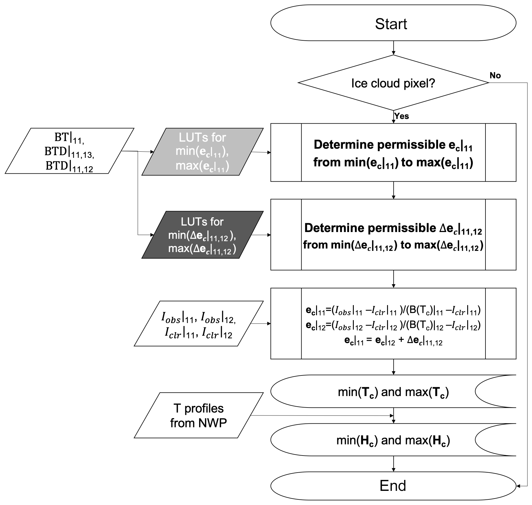
Figure 3 A flowchart for estimation of T_c and H_c corresponding to e_c (from a light gray box that will be shown in Fig. 4) and Δe_c (from a dark gray box that will be shown in Fig. 5), which represent cloud microphysics uncertainty in a certain cloud thickness. We denoted functions for minimum–maximum values of a matrix, A, as min–max(A).

The first step in the current method (Fig. 3) is to constrain 11 µm cloud emissivity ranges (e_c|11) that an ice cloud pixel can have based on the brightness temperatures. To obtain a reasonable e_c|11 boundary corresponding to the ice cloud microphysical properties, the LUTs are generated to provide e_c|11 ranges characterized by brightness temperature (BT) for 11 µm (BT_|11) and BT differences (or BTD) between 11 and 13 µm (BTD${}_{|\mathrm{11},\mathrm{13}}$) and between 11 and 12 µm (BTD${}_{|\mathrm{11},\mathrm{12}}$) (the light gray box in Fig. 3).

The second step is to constrain cloud emissivity differences between 11 and 12 µm for an ice cloud pixel, $\mathrm{\Delta }{e}_{\mathrm{c}|\mathrm{11},\mathrm{12}}$, that are also provided in LUTs (the dark gray box in Fig. 3) with identical input parameters as in the first step. The third step is to find T_c values satisfying the three equations, i.e., Eq. (2) at 11 µm, Eq. (2) at 12 µm, and the equation for cloud emissivity differences (Eq. 4) between 11 and 12 µm with constraints in e_c|11 and $\mathrm{\Delta }{e}_{\mathrm{c}|\mathrm{11},\mathrm{12}}$. That is, the last equation among the three equations in our method is different from Inoue's method (Eq. 5), where

$$\begin{array}{}\text{(6)}& e_{\mathrm{c}|\mathrm{11}}=e_{\mathrm{c}|\mathrm{12}}+\mathrm{\Delta }{e}_{\mathrm{c}|\mathrm{11},\mathrm{12}}.\end{array}$$

The initial assumed 11 µm cloud emissivity begins with a value of min(e_c|11) and increases by a value of 0.01 until T_c converges. Notice that the T_c value, an element of available ice cloud temperatures set as T_c, depends on $\mathrm{\Delta }{e}_{\mathrm{c}|\mathrm{11},\mathrm{12}}$ in Eq. (4). That is, we obtain two T_c values as the minimum and maximum temperatures that an ice cloud pixel can have, corresponding to min–max($\mathrm{\Delta }{e}_{\mathrm{c}|\mathrm{11},\mathrm{12}}$). Finally, we estimate cloud height ranges, H_c, relating to min–max(T_c) using a dynamical lapse rate calculated from GFS NWP temperature profiles provided for 26 isobar layers. The dynamical lapse rate on each grid is calculated from differences in temperatures between 200 and 400 hPa per difference in height between 200 and 400 hPa. In this study, no cloud heights are allowed to be higher than the tropopause, which is provided in the GFS NWP model product.

3.2 Generation of look-up tables (LUTs)

For our method, relevant information for the western North Pacific Ocean is stored in look-up tables (LUTs). The LUTs include the min–max(e_c) and min–max(Δe_c) values for three indices: BTD${}_{|\mathrm{11},\mathrm{13}}$, BTD${}_{|\mathrm{11},\mathrm{12}}$, and BT_|11. The reason for selecting these three indices is that they are linked with cloud optical thickness, cloud effective radius, and cloud temperatures, respectively. Both solar and infrared radiances have been used to investigate cloud microphysics using passive satellite measurements (e.g., Freud et al., 2008; Lensky and Rosenfeld, 2006; Martins et al., 2011). A primary benefit of using IR measurements is that the ice cloud temperature and emissivity do not depend on solar illumination, so the cloud properties are consistent between day and night.

First, the BTD${}_{|\mathrm{11},\mathrm{13}}$ is sensitive to the presence of mid- to high-level clouds and the cloud height. While both the 12 and 13.3 µm measurements are both affected by CO₂ absorption, the 12 µm channel is at the wing of the broad 15 µm CO₂ band and has less CO₂ absorption than the 13.3 µm channel. Additionally, the peak of weighting function for the 13.3 µm channel is in the vicinity of 700–800 hPa so that the observed radiance at 13.3 µm represents the lower-tropospheric temperature. Thus, the BT at 13.3 µm is generally colder than that of the two other IR window channels. The BTD${}_{|\mathrm{11},\mathrm{13}}$ is larger for clear-sky pixels than for ice clouds, but BTD${}_{|\mathrm{11},\mathrm{13}}$ depends on degree of cloud opacity. The BTD${}_{|\mathrm{11},\mathrm{13}}$ has been applied by Mecikalski and Bedka (2006) to monitor changes in cloud thickness and height for signals of convective initiation.

Second, the BTD${}_{|\mathrm{11},\mathrm{12}}$ depends in part on the microphysics and cloud opacity, i.e., the number and distribution of the ice particles; the imaginary part of the refractive index for ice varies in the IR region under study. The BTD${}_{|\mathrm{11},\mathrm{12}}$ has been used to identify cloud type (Inoue, 1985; Pavolonis and Heidinger, 2004; Pavolonis et al.,2005). Prata (1989) used the BTD${}_{|\mathrm{11},\mathrm{12}}$ to discern volcanic ash from nonvolcanic absorbing aerosols. Recently, adding BTD from 8.6 and 11 µm, the BTD${}_{|\mathrm{11},\mathrm{12}}$ is also applied to infer cloud phase (Strabala et al.,1994; Baum et al., 2000, 2012).

Finally, BT_|11 values can provide cloud height information, at least for optically thick clouds including low-level clouds. For optically thick clouds, the BT_|11 values approximate the actual cloud temperature since at 11 µm the primary absorber is water vapor and there is generally little absorption above high-level ice clouds. As noted earlier, the BT_|11 for optically thin clouds includes a contribution from upwelling radiances from the surface and lower atmosphere.

The LUTs are compiled for e_c and Δe_c by three input parameters, i.e., BTD${}_{|\mathrm{11},\mathrm{13}}$, BTD${}_{|\mathrm{11},\mathrm{12}}$, and BT_|11 from information in the C6 MODIS products. Data used in generating our LUTs are summarized in Table 1. The first step is to collect all ice cloud radiances at 11, 12, and 13.3 µm from MYD021KM over the western North Pacific Ocean during the recurring period of August 2013 and 2014. Ice cloud pixels are identified by the MODIS IR cloud thermodynamic phase product in MYD06 (Baum et al., 2012) and where the pixels have a cloud-top temperature ≤260 K. The spatial and temporal domain is restricted to obtain a clear relationship between spectral cloud emissivity and three IR parameters for the case study analyses that will be presented in Sect. 4.

Table 2 Parameter ranges and discretization of parameters in the LUTs for e_c (Fig. 4) and Δe_c (Fig. 5).

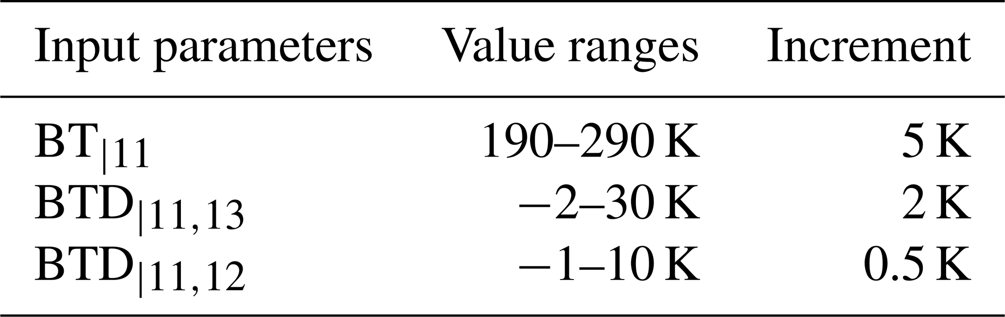
The second step is to categorize the ensemble of ice cloud pixels by three parameters, BTD${}_{|\mathrm{11},\mathrm{13}}$, BTD${}_{|\mathrm{11},\mathrm{12}}$, and BT_|11. The collected cloud pixels are separated into cloud types linked with cloud microphysical properties. We convert radiances centered at 11, 12, and 13.3 µm to BT by the inverse Planck's function and then calculate BTD${}_{|\mathrm{11},\mathrm{13}}$, BTD${}_{|\mathrm{11},\mathrm{12}}$, and BT_|11 for each pixel. Subsequently the ice cloud pixels are sorted into range bins defined for the three parameters as follows: BT_|11 values in a range from 190 to 290 K in increments of 5 K, BTD${}_{|\mathrm{11},\mathrm{13}}$ values in a range from −2 to 30 K in increments of 2 K, and BTD${}_{|\mathrm{11},\mathrm{12}}$ values ranging from −1 to 10 K in increments of 0.5 K (Table 2). For example, the first category is 190 K ≤ BT_|11 < 195 K, −2 ≤ BTD${}_{|\mathrm{11},\mathrm{13}}$ < 0, and −1 ≤ BTD${}_{|\mathrm{11},\mathrm{12}}$ < −0.5.

The final step is to find the possible ranges of e_c and Δe_c in each of the bins of BTD${}_{|\mathrm{11},\mathrm{13}}$, BTD${}_{|\mathrm{11},\mathrm{12}}$, and BT_|11. Here we use the cloud emissivity values at 11 and 12 µm for each ice cloud pixel provided in MYD06, for which the Scientific DataSet (SDS) names are “cloud_emiss11_1km” and “cloud_emiss12_1km”. The cloud emissivity for a single band is obtained by the following equation:

$$\begin{array}{}\text{(7)}& e_{\mathrm{c}}=(I_{\mathrm{obs}}-I_{\mathrm{clr}})/(I_{\mathrm{ac}}+T_{\mathrm{ac}}B\left(T_{\mathrm{c}}\right)-I_{\mathrm{clr}}).\end{array}$$

In Eq. (7), T_ac and I_ac are the above-cloud transmittance and the above-cloud emission (Baum et al., 2012), which are additional terms compared to the definition of the cloud emissivity in the infrared window regions in this paper (Eq. (2). In spite of s different definition of Eq. (7) from the Eq. (2), we use this cloud emissivity data since there the differences are small from the two different equations in the infrared window region. Note that the cloud emissivity data from C6 MYD06 are retrieved under the assumption of the single-layered cloud. Here the possible ranges of e_c and Δe_c are determined as the min–max(e_c) and (Δe_c) among cloud emissivity values allocated by the bins of three parameters. To exclude extreme values, the min–max(e_c) and (Δe_c) are defined as the 2nd and 98th percentiles of the e_c and Δe_c distributions when there are at least 5000 pixels available for a given bin. When there are between 500 and 5000 pixels, the 5th and 95th percentiles are chosen as the min–max(e_c) and (Δe_c). In the rare case when there are between only 200 and 500 pixels, the 10th and 90th percentiles are used. Any case with fewer than 200 ice cloud pixels is not included in the LUTs.

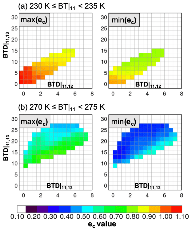
Figure 4 Look-up table values for min–max(e_c) (left and right panels in colors) by BTD${}_{|\mathrm{11},\mathrm{12}}$ (x axis) and BTD${}_{|\mathrm{11},\mathrm{13}}$ (y axis) for (a) 230 K ≤ BT_|11 < 235 K and (b) 270 K ≤ BT_|11 < 275 K. For this look-up table, ice cloud pixels with temperatures ≤260 K were collected from MODIS C6 over the western North Pacific Ocean during two Augusts (2013–2014). Table 1 summarizes data used in the look-up table. Also, Table 2 is for dimensions of the look-up table.

Figure 4 shows examples of LUT values for e_c belonging to the specific category for 230 K ≤ BT_|11 < 235 K (Fig. 4a) and 270 K ≤ BT_|11 < 275 K (Fig. 4b), which imply the presence of optically thick and thin ice clouds, respectively. The minimum (the left panel) and maximum (the right panel) values of the e_c are shown as colors in the space of BTD${}_{|\mathrm{11},\mathrm{12}}$ (x axis) and BTD${}_{|\mathrm{11},\mathrm{13}}$ (y axis). In Fig. 4a, the e_c values range from about 0.8 to 1.1. The e_c generally ranges from 0 to 1, but a nonphysical e_c value over 1 might occur in the case of an overshooting cloud (from strong convection that briefly enters the lower stratosphere) that has a colder temperature than the surrounding environment temperature (Negri, 1981; Adler et al., 1983). As for optically thin clouds, the e_c values of Fig. 4b range from around 0.3 to 0.8. In general, e_c values are low when cloudy pixels have large values of BTD${}_{|\mathrm{11},\mathrm{12}}$ and BTD${}_{|\mathrm{11},\mathrm{13}}$.

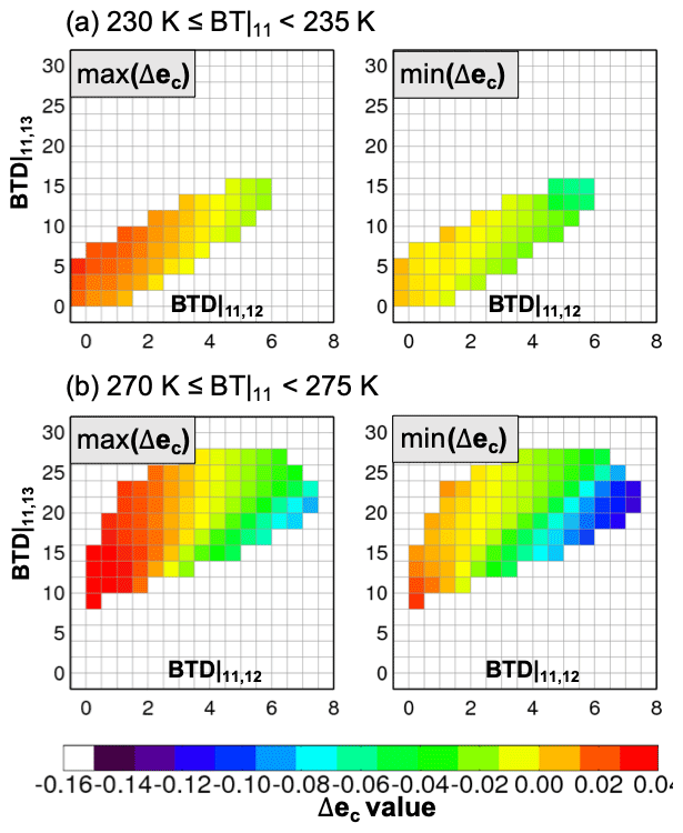
Figure 5 Look-up tables for min–max(Δe_c) (left and right panels in colors) by BTD${}_{|\mathrm{11},\mathrm{12}}$ (x axis) and BTD${}_{|\mathrm{11},\mathrm{13}}$ (y axis) for (a) 230 K ≤ BT_|11 < 235 K and (b) 270 K ≤ BT_|11 < 275 K. Identical data as in Fig. 4 are used to generate these look-up tables, except that cloud emissivity differences between 11 and 12 µm come from MODIS C6 (referring to Tables 1 and 2).

Figure 5 shows examples of LUT values of Δe_c for optically thick (Fig. 5a) and thin (Fig. 5b) ice clouds as shown in Fig. 4. The Δe_c ranges from −0.12 to 0.04. The Δe_c shows a more complex relationship with BTD${}_{|\mathrm{11},\mathrm{12}}$ and BTD${}_{|\mathrm{11},\mathrm{13}}$ than with e_c. It is notable that similar patterns Δe_c are repeated on the optically thick (Fig. 5a) and thin ice cloud (Fig. 5b). One reason for this could be that Δe_c values are more sensitive to particles sizes, whereas e_c values are more directly linked with cloud opacity (refer to Eqs. 3 and 4). The optically thin ice cloud cluster tends to be more sensitive to BTD${}_{|\mathrm{11},\mathrm{12}}$, showing larger variations in Δe_c than the thick ice cloud cluster.

4 Results

The current algorithm analyses are performed over the study domain, the western North Pacific Ocean, in August 2015. Note that the Typhoon Goni formed on 13 August and dissipated on 30 August 2015, and affected East Asia. Case studies involving Typhoon Goni scenes are provided in Sect. 4.1. Quantitative analysis and comparison of our results with CALIOP cloud products are described in Sect. 4.2.

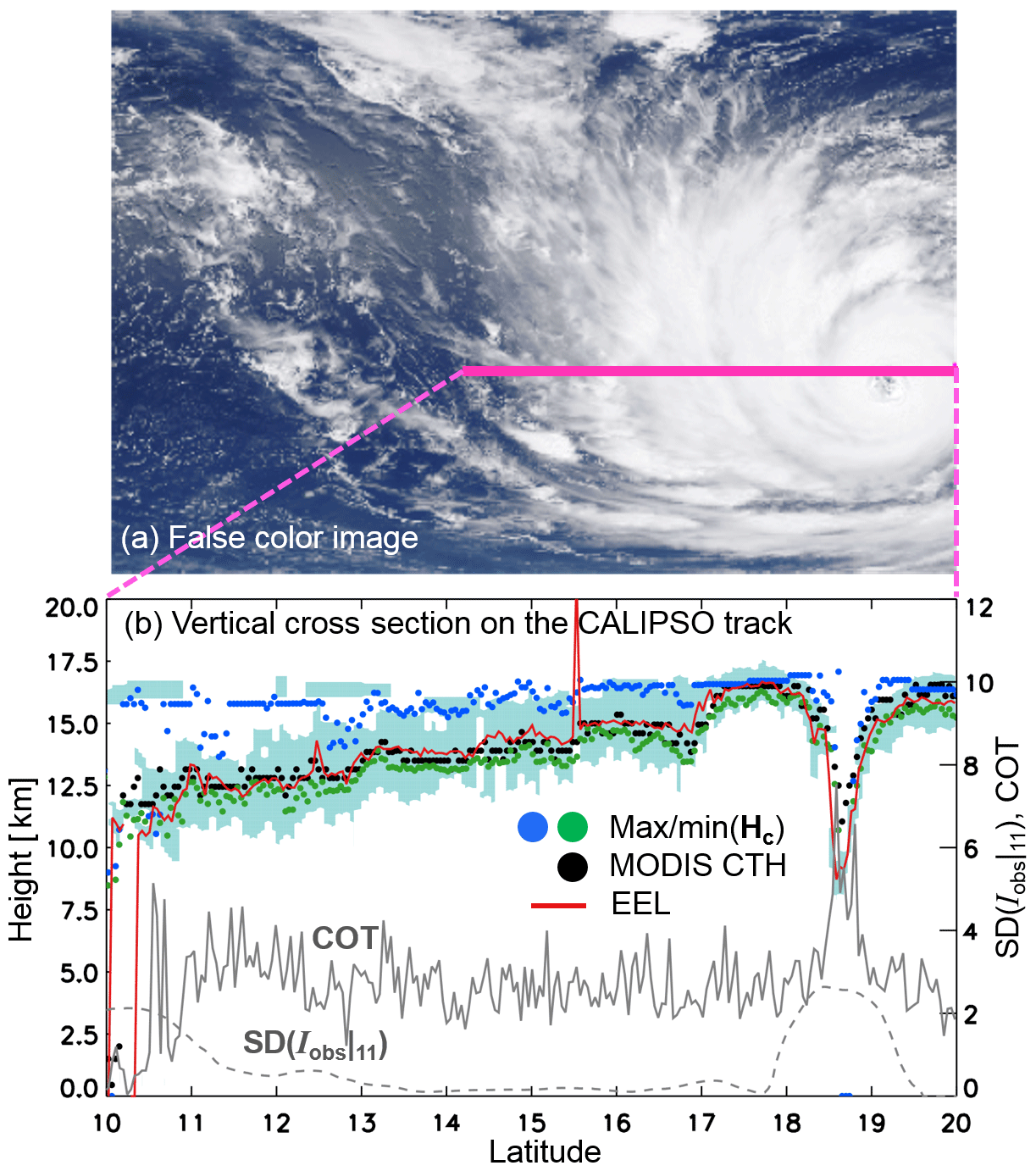
Figure 6 (a) MODIS false color image (rotated 90^∘ left) at 03:20 UTC on 19 August 2015. This scene captures part of Typhoon Goni. The heavy pink line on the image shows the CALIPSO track the closest to MODIS observation time. (b) Vertical cross section of the CALIPSO track designated by the heavy pink line in Fig. 6a. The vertical feature mask is shown as sky-blue contours (randomly and horizontally oriented ice). The red solid line shows where the layer COT (integrated Q_e at 532 nm from CALIOP) reaches a value of 0.5. The green–blue and black circles are the min–max(H_c) and MODIS CTH, respectively. The gray solid (dashed) line on the right-side y axis is the column COT from CALIOP (standard deviation of 11 µm radiances from MODIS).

Table 3 Data used for the tests shown in Fig. 3. Input and auxiliary data are taken from the MODIS C6 cloud products and from CALIOP v4 cloud products. The abbreviations CTT–CBT, CTH–CBH, COT, T–P, and VFM refer to cloud-top and cloud-base temperature, cloud-top and cloud-base height, cloud optical thickness, temperature and pressure, and vertical feature mask. The vertical profile of the extinction coefficient at 532 nm is denoted as the Q_e.

4.1 Comparison of min–max(H_c) with CALIPSO for three granules

4.1.1 A scene for single-layered optically thin ice clouds (19 August 2015, at 03:20 UTC)

Figure 6 is a scene analysis for single-layered optically thin ice clouds for a granule at 03:20 UTC on 19 August 2015. Figure 6a is a MODIS false color image that captures Typhoon Goni. Note that the image is rotated 90^∘ left to simplify comparison with CALIPSO. The heavy pink line (Fig. 6a) is the south-to-north CALIPSO track at the closest time to the MODIS observation time. CALIPSO made a near-eye overpass of the cyclone. The CALIOP track measures a cross section of the cyclone, from the eye wall to the outer bands. Figure 6b is a cross section from CALIOP data (Table 3) at the time of the overpass that shows the horizontal (x axis) and vertical (y axis at the left side) locations of all cloud layers. The CALIOP vertical feature mask (VFM) indicates the presence of randomly oriented ice and horizontally oriented ice (sky blue) in the scene. The y axis at the right side is for two supplementary data shown as gray lines. The gray solid line is the CALIOP COT at 532 nm, for the opacity of ice clouds. The gray dashed line is the standard deviation of the MODIS I_obs|11 (SD(I_obs|11)) on the collocated path with the CALIOP track, calculated over a 5×5 pixel array centered at each cloud pixel. The SD(I_obs|11) includes cloud feature information (Nair et al., 1998). For example, pixels at cloud edges or fractional clouds have relatively large SD(I_obs|11). The SD(I_obs|11) values are used to filter overcast cloud pixels. The data in Fig. 6 are primarily of single-layered ice clouds with horizontal homogeneity as demonstrated by the low value of SD(I_obs|11).

For comparison with CALIPSO, the min–max(T_c) values are converted to max–min(H_c) and are shown from our method (blue and green circles) to the VFM in Fig. 6b. Also provided is the MODIS CTH (black circles) for reference. For these comparisons, we converted temperature to height using a dynamical lapse rate from GFS NWP temperature profiles. When the cloud pixel temperature is colder than the tropopause temperature, it is changed to be that of the tropopause and is converted to the tropopause height provided by GFS NWP. The solid red line indicates where the CALIOP COT is about 0.5. This line is a reference for the position where the passive remote sensing retrievals will place the cloud (Holz et al., 2006; Wang et al., 2014), well known as the radiative emission level. The radiative emission level should be thought of more as a guideline since the matched COT values can be different depending on cloud types or algorithm methods. To determine this depth in the cloud layer, we integrated the extinction coefficient, CALIOP Q_e (Table 3), from the top of the cloud downwards until the COT reached about 0.5. Hereafter, we call that layer the effective emission layer, EEL. The enhancement of EEL at approximately 15.6^∘ N in Fig. 6b is caused by an extraordinary value of Q_e provided in CALIOP v4.

Note that the max(H_c) (blue circles) is close to the top of the clouds except in the region of cloud edges and the eye of Goni. Bias between the cloud top and the max(H_c) is 0.46 km, that is −4.5 K in the aspect of temperature. It is remarkable that the max(H_c) corresponding to uncertainties of cloud emissivity tends to occur at or slightly above the cloud top as indicated by CALIPSO, higher than the EEL and MODIS CTH. The height of the min(H_c) (green circles) also follows the base of the cloud layer with a bias of −1.58 km (10.6 K in temperature), slightly lower than EEL and MODIS CTH. These results show the feasibility of inferring single-layered ice cloud boundaries from spectral cloud emissivity and its uncertainties by IR measurements. The max–min(H_c) on the cloud edges and the edges surrounding the eye of the Goni have relatively large biases from the top and base of the cloud. Those regions show relatively large SD(I_obs|11) and small COT and contain multiple clouds. To sum up, our resulting cloud heights corresponding to cloud emissivity uncertainties are likely to exhibit similar variations to the CALIOP VFM, except the cloud edges and multiple cloud regions.

Figure 7 (a) BT_|11 image from MODIS (MYD021 C6) at 15:30 UTC on 19 August 2015. This scene captures part of Typhoon Goni. The heavy pink line on the BT_|11 image shows the CALIPSO track the closest to MODIS observation time. (b) Vertical cross section of the CALIPSO track designated by the heavy pink line in Fig. 7a. The vertical feature mask is shown as sky-blue contours (randomly and horizontally oriented ice). The red solid line shows where the layer COT (integrated Q_e at 532 nm from CALIOP) reaches a value of 0.5. The green–blue and black circles are the min–max(H_c) and MODIS CTH, respectively. The gray solid (dashed) line on the right-side y axis is the column COT from CALIOP (standard deviation of 11 µm radiances from MODIS).

4.1.2 A scene for single-layered optically thick ice clouds (19 August 2015, at 15:30 UTC)

The second case is the single-layered optically thick ice clouds (Fig. 7) at 15:30 UTC on 19 August 2015. Here we show the BT_|11 image instead of RGB image (Fig. 7a) since this is a nighttime scene. Figure 7a is also rotated 90^∘ left. For this overpass, CALIOP-observed clouds farther away from the center of Goni, and inspection of the cross section in Fig. 7b suggests that most of cloud pixels are optically thick with COT values higher than 5, about where the CALIOP signal attenuates, and have relatively low SD(I_obs|11) as indicated by the gray solid and dashed lines in Fig. 7b. In the comparison with the CALIOP VFM, the max(H_c) tends to occur at or slightly below the cloud top as indicated by CALIPSO, still higher than the EEL and MODIS CTH. The bias for the max(H_c) from the top of clouds is 2.38 km (−13.2 K), which is larger than that of optically thin ice clouds. The bias for min(H_c) from the cloud base is larger than that of optically thin clouds, −2.69 km (19.4 K), but the min(H_c) still exhibits similar variation to CALIOP VFM. The passive IR measurements have an upper COT limit as shown in earlier studies (Heidinger et al., 2009, 2010). The height boundaries from our method brackets both the CALIPSO measurements and the MODIS retrievals.

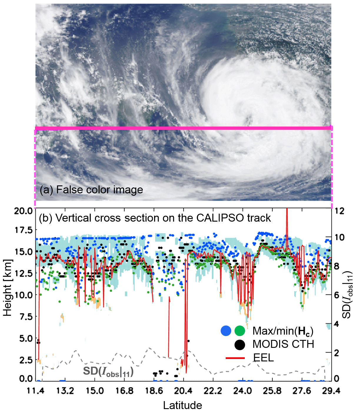
Figure 8 (a) MODIS false color image (rotated 90^∘ left) at 05:20 UTC on 8 August 2015. This scene captures part of Typhoon Goni. The heavy pink line on the image shows the CALIPSO track the closest to MODIS observation time. (b) Vertical cross section of the CALIPSO track designated by the heavy pink line in Fig. 8a. The vertical feature mask is shown as sky-blue and orange contours (randomly and horizontally oriented ice and water). The red solid line shows where the layer COT (integrated Q_e at 532 nm from CALIOP) reaches a value of 0.5. The green–blue and black circles are the min–max(H_c) and MODIS CTH, respectively. The gray solid (dashed) line on the right-side y axis is the column COT from CALIOP (standard deviation of 11 µm radiances from MODIS).

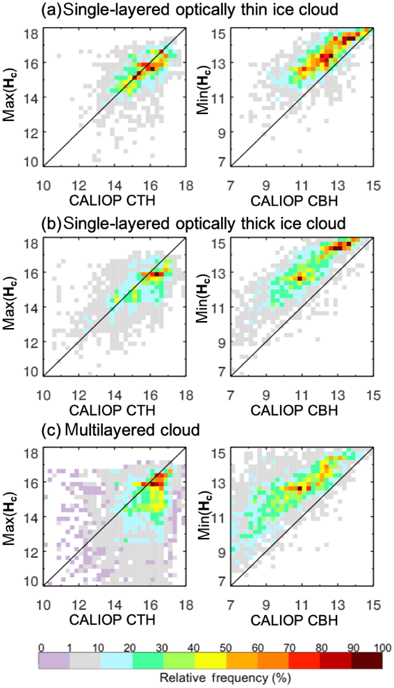
Figure 9 Joint histograms of three cloud categories: (a) single-layered optically thin ice cloud, (b) optically thick ice cloud, and (c) multilayered cloud during August 2015. The first column shows CALIOP CTH (cloud-top height, x axis) versus max(H_c) (y axis), the second column shows CALIOP CBH (cloud-base height, x axis) versus min(H_c) (y axis).

4.1.3 A scene for multilayered cloud (8 August 2015, at 05:20 UTC)

The third case also involves a cross section of Goni, but this scene is more complex in that there is evidence of both multilayered and less homogeneous ice clouds on the southern boundary of the typhoon (Fig. 8a). Note that the SD(I_obs|11) on the CALIPSO track shows relatively large variances, compared to the previous two cases (Fig. 8b). The CALIOP COT is omitted given the high fluctuations in the values. The CALIOP vertical feature mask (VFM) indicates the presence of randomly oriented ice and horizontally oriented ice (sky-blue) including water (orange) cloud phase. The enhancement of EEL at around 25.7^∘ N in Fig. 8b is also caused by an extraordinary value of Q_e provided in the CALIOP v4 product. In the region of 10–20^∘ N, the max–min(H_c) values in this region are often outside the boundaries of the VFM. The max(H_c) (blue circles) varied from near the second cloud layer to the top of the first cloud at the tropopause. Some pixels of the min(H_c) (green circles) values are also outside the range of the VFM. There is more than one reason causing these increased variances, including the fact that the uppermost cloud layer is optically thin (over half of all pixels have COT < 1.5) and there are indications of lower cloud layers. In the region of 20–30^∘ N, clouds on the top layer are relatively thick (on average, COT = 3.5). In that case, heights of the max(H_c) on the multilayer pixels tend to be close to the EEL, which is much lower than the top of clouds. This is to be expected for the case of a geometrically thick but optically thin cloud. Note that the value of the min(H_c) on the multilayered cloud pixels sometimes reaches almost to the second cloud layer, rather than near the first layer. Further thought needs to be given to these cases.

4.2 Comparison of max–min H_c with CALIPSO for August 2015

In this section, the max–min(H_c) is compared with the cloud-top and cloud-base height (CTH–CBH) from CALIOP over the western North Pacific during August 2015. The computationally efficient method of Nagle et al. (2009) is used to collocate the simultaneous nadir observations (SNOs) between two satellites. Following their approach, CALIOP is projected onto MODIS.

First, we qualitatively examine the max–min(H_c) with the cloud layer vertical cross section from CALIOP–MODIS matchup files (Table 3) in Figs. 6–8. Second, we quantitatively investigate the max–min(H_c) for all ice clouds against CALIOP CTH–CBH during the month. The extinction coefficient profiles, cloud phase and their quality flags, and the number of cloud layers are extracted from CALIOP and used in this analysis (Table 3).

The matchup data are filtered as follows: only ice cloud phase pixels are chosen that have the highest quality (CALIOP QC for cloud phase = 1), where CALIOP COT > 1.5 and SD(I_obs|11) from MODIS ≤ 1, which helps to remove cloud edges and fractional clouds. The relationship is investigated between the max–min(H_c) and CALIOP CTH–CBH for three cloud regimes: (1) single-layered optically thin ice clouds, (2) optically thick ice clouds, and (3) multilayered clouds where the uppermost layer is optically thin cirrus. The CALIOP–MODIS matchup clouds are separated into single-layered and multilayered cloud groups using the number of layers found (NLF) from CALIOP (Table 3). The multilayered cloud group includes two or more cloud layers, excluding single-layered clouds. Among single-layered cloud pixels, we define optically thin and thick cloud groups as CALIOP COT, which is less and greater than 3.5, referring to the ISCCP cloud classification (Rossow et al., 1985; Rossow and Schifer,1999).

Table 4 Comparison of max(H_c) (min(H_c)) to the CALIOP CTH (CALIOP CBH) for all cloud pixels and three cloud regimes; single-layered optically thin ice cloud, optically thick ice cloud, and multilayered cloud for August 2015. Pixel numbers (count), correlation coefficients (corr) and differences of the mean values (bias), and root-mean-square differences (rmsd) are provided. Additionally, comparison of min–max(T_c) to the CALIOP CTT–CBT is also shown as numbers in round brackets.

Figure 9 shows the joint histogram of the max–min(H_c) (y axis of left and right panels) as a function of the CALIOP CTH–CBH (x axis) for single-layered optically thin ice cloud (Fig. 9a), single-layered optically thick ice cloud (Fig. 9b), and multilayered clouds (Fig. 9c). Table 4 provides all statistical quantities for Fig. 9 as correlations (corr), differences of the mean value (bias), and root-mean-square differences (rmsd). Additionally, all statistical quantities in terms of temperature are in kelvin and are given in the round brackets in Table 4. For single-layered clouds, the majority of max(H_c) values are scattered about the one-to-one line. The statistical values are corr = 0.61, bias = 0.13 km, and rmsd = 0.91 for thin clouds. This implies that the maximum values of cloud height ranges corresponding to e_c and Δe_c are close to the cloud top for single-layered clouds as determined from CALIOP.

However, the scatter is higher for optically thick clouds, with corr = 0.65, bias = 0.30 km, and rmsd = 1.08 (Table 4). As for the max(H_c) for multilayered clouds, the majority of scatter points are on the lower right side of the one-to-one line, with corr = 0.25, bias = 1.41 km, and rmsd = 2.64. The lowest correlation and the largest bias for multilayered clouds are shown, as expected given the assumption of the single-layered clouds in our method.

The comparisons of the min(H_c) (y axis of right panels in Fig. 9) to the CALIOP CBH (x axis) for all cloud categories show relatively large correlations, at least over 0.48. Scatter points in three joint histograms for all cloud types are parallel to the one-to-one line, but show negative biases implying higher heights than CALIOP CBT. As with the cases of the max(H_c), bias of the min(H_c) increases from single-layered optically thin ice (−1.01 km) to optically thick ice (−1.71 km) and multilayered clouds (−4.64 km).

5 Discussion of results

The results in Figs. 6–9 show the comparisons of the ice cloud height ranges obtained based on the ice cloud emissivity uncertainties with both MODIS C6 products and vertical cross sections of clouds from CALIOP. We investigated minimum and maximum ice cloud heights for each cloud pixel for three cloud regimes during August 2015: (1) single-layered optically thin clouds, (2) optically thick ice clouds, and (3) multilayered clouds.

Overall, the maximum values of the estimated ice cloud height ranges for single-layered optically thin and thick ice clouds show some skill in comparison with the cloud tops from CALIOP: corr = 0.61 and 0.65 as well as bias = 0.13 and 0.30 km. In particular, we note that the upper height boundary for optically thin clouds derived from our method is very close to the geometric cloud tops. For multilayered clouds, the maximum heights are occasionally much lower than the uppermost cloud layer as observed by CALIOP, showing the highest bias at 1.41 km. Higher biases are expected in our method given the assumption of single-layered clouds in each pixel. Additionally, the skill of our method decreases when the upper cloud layer is composed of optically thin (having very low COT values) and fractional clouds; in some cases, the method cannot determine an emissivity range from the LUTs, which were generated for single-layered ice clouds.

The minimum heights for single-layered optically thin ice clouds reach near the base of the cloud, with corr = 0.83 and bias = −1.01 km. However, for thick and multilayer, the biases became larger, at most –4.64 km. That is, the minimum heights for thick clouds became much higher than the CALIOP-observed cloud bases. This indicates that the IR method has an optical thickness limitation and is more useful for lower optical thicknesses, which has been noted previously (e.g., Heidinger et al., 2010). Even with large biases of minimum heights, it is notable that correlation coefficients between minimum heights and the cloud base for all three cloud regimes are sufficiently large, at least 0.48.

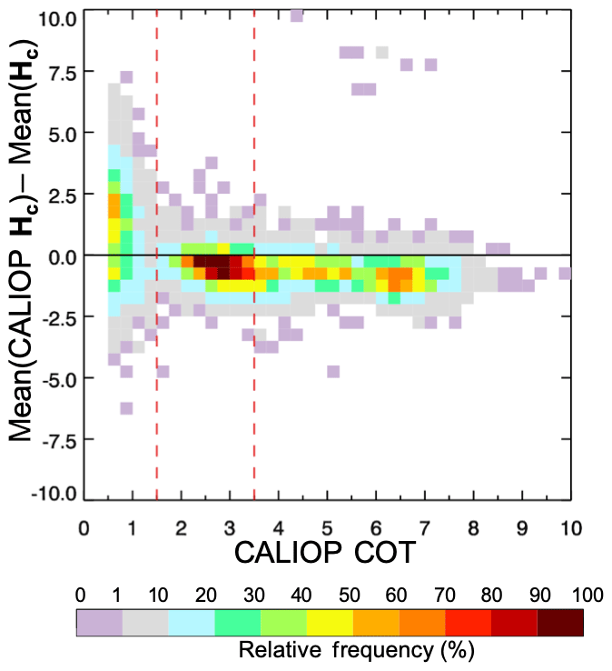
Figure 10 A frequency of biases of mean(H_c) from mean(CALIOP H_c) as a function of CALIOP COT during August 2015. The mean(CALIOP H_c) implies the average of the upper and lower cloud boundaries, simply defined as $\mathrm{0.5}\cdot (\text{CALIOP CTH}+\text{CALIOP CBH})$. The mean(H_c) is also the average of cloud heights by our method, defined as $\mathrm{0.5}\cdot (min(H_{\mathrm{c}})+max(H_{\mathrm{c}}\left)\right)$. The red dotted lines are references for single-layered optically thin (1.5 < COT ≤ 3.5) and optically thick (COT > 3.5) ice clouds in this study.

To better understand the potential biases of the current algorithm in comparison with CALIOP, we compare the mean(H_c) to the mean(CALIOP H_c) that are defined as $\mathrm{0.5}\cdot \left(\text{max}\right(H_{\mathrm{c}})+\text{min}(H_{\mathrm{c}}\left)\right)$ and as $\mathrm{0.5}\cdot (\text{CALIOP CTH}+\text{CALIOP CBH})$, respectively. Figure 10 shows the frequency of occurrence of biases, that is, the mean(CALIOP H_c) minus the mean(H_c), as a function of CALIOP COT for the single-layered ice clouds during August 2015. In a comparison of the MODIS cloud mask with CALIOP, Ackerman et al. (2008) noted that the cloud mask performs best at optical thicknesses above about 0.4. The lidar has a greater sensitivity to particles in a column than passive radiance measurements. Based on this consideration, we limited our results to those pixels where the COT ≥0.5 on the x axis of Fig. 10.

Figure 10 illustrates that our resulting single-layered ice cloud boundaries are consistent with CALIOP measurements, showing slightly negative biases except for the region near “COT ≤ 1.5”. These results suggest that our approach for applying a range of cloud emissivity values to estimate cloud boundaries has potential merit for using IR channels to produce cloud boundaries similar to those that the lidar observes, especially for optically thin but geometrically thick ice clouds which tend to have large uncertainties (Hamann et al., 2014).

The negative biases of the mean(H_c) from CALIOP measurements are caused primarily by two factors: (1) the min(H_c) values for all cloud regimes tend to be higher than the geometric cloud base, and (2) the max(H_c) values are sometimes slightly outside the actual cloud boundaries. Perhaps this is caused in part by the conversion of temperature to height using the NWP model product. Another source of error could be that the radiances have some amount of uncertainty that was not considered in our methodology. A notable point is that the boundary heights for optically thin cirrus (1.5 < COT ≤ 3.5) show the lowest biases.

Figure 10 also addresses the weaknesses of our method. In the region of COT ≤ 1.5, biases of mean(H_c) from CALIOP are largest and positive. This region might be relevant to fractional clouds or cloud edges. We infer that the relationship of cloud emissivity at 11 and 12 µm, the key controller in our method, might not be optimal in the fractional clouds or cloud edges, resulting in lower heights.

A limitation of this study is that the LUTs are generated for spectral emissivity using IR sensor observations and level-2 products that still have errors and uncertainties. It would be interesting to extend this preliminary research by generating LUTs for spectral emissivity using CALIOP, not IR sensors. If we can obtain more diverse ice cloud emissivity in vertical cloud thickness, it could result in improvements in the resulting cloud temperatures and height ranges. Also, the LUTs based on CALIOP data/products could be used to reduce errors in inferring cloud temperatures for multilayered clouds.

6 Summary

The intent of our study is to demonstrate that ice cloud emissivity uncertainties, obtained from three IR channels generally available on various satellite-based sensors, can be used to estimate a reasonable range of ice cloud temperatures as verified through comparison with active measurements from CALIPSO. For satellite-based retrievals with heavy data volumes, the general assumption is that the cloud in any given pixel can be treated as plane parallel, which simplifies the retrieval algorithms. However, for ice clouds and particularly optically thin ice clouds known as cirrus, the plane-parallel assumption breaks down because cirrus tends to be optically thin but geometrically thick, which is different with lower-level liquid water clouds. For cirrus, the inference of a cloud-top temperature for a given measurement may not be optimal. In our approach, a range of spectral ice cloud emissivity is calculated, which is, in turn, used to infer a range of cloud temperatures. These temperatures are converted to heights and subsequently compared to active lidar measurements provided by CALIPSO CALIOP products.

This study provides a methodology to infer a range of spectral cloud emissivity for each cloud pixel. The range in emissivity represents uncertainty in the cloud microphysics to some degree. In our approach, we generate two LUTs for cloud emissivity at 11 µm and cloud emissivity differences between 11 and 12 µm using the brightness temperatures at 11, 12, and 13.3 µm. The 11 µm channel is a window channel where the primary absorption is caused by water vapor. The 12 µm channel is impacted by both H₂O and CO₂, while the 13.3 µm channel has more absorption by CO₂ than by water vapor. The benefit of a method that relies on IR channels is that it does not depend on solar illumination, so the cloud heights can be obtained consistently between day and night.

We estimate a range of ice cloud temperature corresponding to the ice cloud uncertainty generated by three IR channels centered at 11, 12, and 13.3 µm by MODIS C6. The focus area is the western North Pacific Ocean during August 2015. We verified the estimated ranges of ice cloud temperature for three cloud categories, i.e., single-layered optically thin ice and optically thick ice clouds and multilayered clouds, against the vertical feature mask for CALIOP. We show that the minimum–maximum values for the estimated range of ice cloud heights agree with CALIPSO measurements fairly well for single-layered optically thin clouds. However, for optically thick and multilayered clouds, the biases of the minimum–maximum values for those ranges from the cloud top and cloud base became larger.

This approach can be applied to the new geostationary satellites, such as Himawari-8 (launched in 2015), GOES-16/17 (launched in 2016 and 2017), and GK-2A (launched in 2018). The new features of ice cloud temperatures from base to top by geostationary IR observation could contribute to improved accuracy of weather prediction and cloud radiative effects.

In future work, we intend to improve upon this methodology by developing lookup tables for spectral cloud emissivity uncertainty with CALIOP. Above all, it is required to study for global area for applying this method to the new geostationary satellites. Also, further study is required to add more infrared channels to resolve more accurate spectral cloud emissivity uncertainties.