the Creative Commons Attribution 4.0 License.
the Creative Commons Attribution 4.0 License.
 | 23 Sep 2019
Toward autonomous surface-based infrared remote sensing of polar clouds: retrievals of cloud optical and microphysical properties
Christopher J. Cox
Steven Neshyba
Von P. Walden
Improvements to climate model results in polar regions require improved knowledge of cloud properties. Surface-based infrared (IR) radiance spectrometers have been used to retrieve cloud properties in polar regions, but measurements are sparse. Reductions in cost and power requirements to allow more widespread measurements could be aided by reducing instrument resolution. Here we explore the effects of errors and instrument resolution on cloud property retrievals from downwelling IR radiances for resolutions of 0.1 to 20 cm−1. Retrievals are tested on 336 radiance simulations characteristic of the Arctic, including mixed-phase, vertically inhomogeneous, and liquid-topped clouds and a variety of ice habits. Retrieval accuracy is found to be unaffected by resolution from 0.1 to 4 cm−1, after which it decreases slightly. When cloud heights are retrieved, errors in retrieved cloud optical depth (COD) and ice fraction are considerably smaller for clouds with bases below 2 km than for higher clouds. For example, at a resolution of 4 cm−1, with errors imposed (noise and radiation bias of 0.2 mW/(m2 sr cm−1) and biases in temperature of 0.2 K and in water vapor of −3 %), using retrieved cloud heights, root-mean-square errors decrease from 1.1 to 0.15 for COD, 0.3 to 0.18 for ice fraction (fice), and 10 to 7 µm for ice effective radius (errors remain at 2 µm for liquid effective radius). These results indicate that a moderately low-resolution, surface-based IR spectrometer could provide cloud property retrievals with accuracy comparable to existing higher-resolution instruments and that such an instrument would be particularly useful for low-level clouds.
- Article
(1605 KB) - Full-text XML
-
Supplement
(3390 KB) - BibTeX
- EndNote


Knowledge of polar cloud properties is critical for understanding climate change in polar regions. Polar regions are among the most rapidly warming regions on Earth, with significant concurrent changes in cloud properties that influence the amount of warming (Wang and Key, 2005) and indications that sensitivity to clouds may increase in a warming Arctic (Cox et al., 2015). Clouds have a strong influence on the polar surface energy budget (Lawson and Gettelman, 2014; van den Broeke et al., 2017), influencing sea ice loss (Francis and Hunter, 2006; Kay and Gettelman, 2009; Wang et al., 2019) and Greenland ice melt (van den Broeke et al., 2017). Despite ongoing efforts to improve cloud processes in climate models, the Intergovernmental Panel on Climate Change (IPCC) finds that “clouds and aerosols continue to contribute the largest uncertainty to estimates and interpretations of the Earth's changing energy budget,” (Boucher et al., 2013). Improving the representation of cloud processes in climate models requires observational constraints, including ice and liquid water paths, particle size, and thermodynamic phase (Komurcu et al., 2014; Winker et al., 2017). This is particularly true for the polar regions, where clouds and cloud processes are distinctly different from lower latitudes and present unique challenges for modeling cloud radiative effects (Hines et al., 2004) and where measurements are sparse.
Although ground-based observations in the polar regions are sparse, measurements made during campaigns and at permanent field sites (e.g., Bromwich et al., 2012; Cox et al., 2014; Uttal et al., 2015, and references therein; Lachlan-Cope et al., 2016; Silber et al., 2018) and from satellites (e.g., L'Ecuyer and Jiang, 2010) have made important contributions to our understanding of polar clouds. IR spectrometers are proven instruments for remote sensing that have been part of many of these surface and satellite-based measurements. Surface-based IR spectrometers are most sensitive to the cloud base, providing an important complement to satellite-based measurements. In particular, Atmospheric Emitted Radiance Interferometer (AERI) instruments currently operate at Barrow (1998–current), Eureka (2006–current), and Summit (June 2010–current): three Arctic intensive observing sites (Uttal et al., 2015). In the Antarctic, there have been only short-term surface-based IR spectrometer measurements, including measurements made at Amundsen–Scott South Pole Station in 1992 (Mahesh et al., 2001) and 2001 (Rowe et al., 2008), at Dome C during Austral summer 2003 (Walden et al., 2005) and 2012–2014 (Palchetti et al., 2015), and at McMurdo (as part of the Atmospheric Radiation measurement (ARM) West Antarctic Radiation Experiment, or AWARE; Silber et al., 2018). These measurements are crucial, but represent only very sparse coverage of the polar regions.
Because IR radiance measurements are passive, the energy requirements are considerably lower than for active instruments such as lidar. Thus there is the potential for portable, low-cost, autonomous IR spectrometers that could be deployed to remote locations to make widespread IR radiance measurements across the polar regions from which cloud properties could be retrieved. Such measurements would be beneficial in a number of ways: First, they could be used to fill gaps in satellite measurements. For example, cloud properties were retrieved at Eureka from 2006 to 2009 from AERI measurements made nearly continuously every ∼40 s (Cox et al., 2014). By contrast, satellite overpasses are typically twice per day. Second, surface-based measurements can be used to validate satellite-based measurements. Finally, surface-based instruments are generally better at characterizing clouds in the boundary layer. To demonstrate the feasibility of such an instrument, the limitations of the retrieval given instrument operational constraints and availability of ancillary data must first be assessed.
In this paper, we explore the accuracy with which cloud properties could be retrieved from a portable IR spectrometer, including optical depth, thermodynamic phase, and effective radius. This paper builds on similar work that explored the accuracy of cloud-height retrievals (Rowe et al., 2016). One way to develop a robust, low-power portable spectrometer might be to reduce the instrument resolution. Here we quantify cloud-property retrieval accuracy as resolution becomes coarser, from 0.1 to 20 cm−1. Cloud properties are retrieved from simulated downwelling radiance spectra using the CLoud and Atmospheric Radiation Retrieval Algorithm (CLARRA). In addition to retrieving cloud height (Rowe et al., 2016), CLARRA retrieves cloud optical and microphysical properties from IR radiances using an optimal inverse method in a Bayesian framework. Cloud property retrievals are performed for simulated polar clouds with varying atmospheric thermal and humidity structure, cloud optical depth (in the geometric limit, hereafter COD), thermodynamic phase (including mixed-phase and supercooled liquid), liquid effective radius, ice effective radius, ice crystal habit, and cloud vertical structure. Mixed-phase clouds were simulated as an external, homogeneous mixture of liquid and ice particles. We also examine the sensitivity of retrieved results to noise and bias imposed on the radiance as well as to errors in specified input parameters, especially the atmospheric state and cloud height.
To test the effect of instrument resolution on the ability to retrieve cloud properties from downwelling radiances, retrievals using CLARRA were performed on a set of simulations. Using simulations rather than actual measurements confers a variety of benefits: (1) the basic capability of the model, in the absence of error, can be determined, setting a benchmark for retrieval capability, (2) the effects of various sources of error (such as noise, bias, or uncertainty in the atmospheric state) can be determined and assessed independently, and (3) errors in the retrieved values are known and thus can be compared to assess the uncertainty prediction from the CLARRA model.
The set of simulated downwelling radiances is described in detail by Cox et al. (2016) and by Rowe et al. (2016). The simulations are based on observed Arctic atmospheric profiles and cloud properties meant to represent a typical Arctic year, based on statistics from field observations (Cox et al., 2016, and references therein; although designed for the Arctic, significant overlap is expected for typical Antarctic atmospheric states, except perhaps in winter in the interior, when the atmosphere is colder and drier). All clouds were modeled as plane-parallel, single-layer clouds. Precipitable water vapor (PWV) varied from 0.2 to 3 cm.
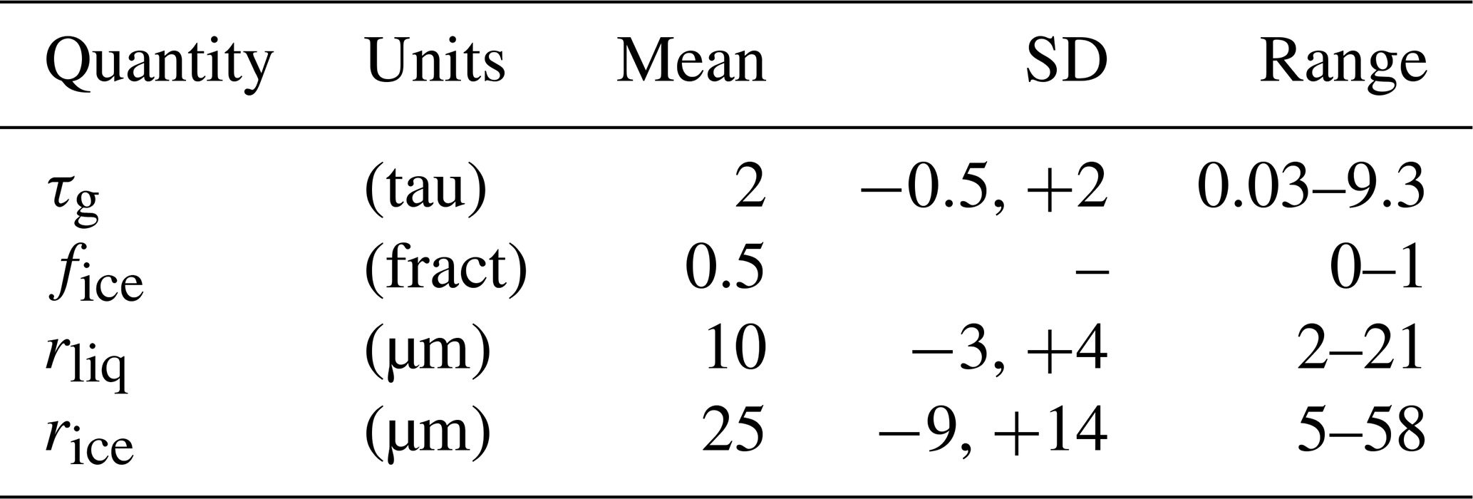
A base set of 222 simulated radiances was created for atmospheres with vertically uniform clouds, using spheres for ice crystal habit (as well as for liquid droplet shape). Cloud bases vary from 0 to 7 km, with about 70 % of clouds within the lowest 2 km and 30 % above; thickness varies from 0.1 to 1.6 km; and temperatures vary from 225 to 282 K. Mixed-phase clouds are modeled as externally mixed and span temperatures of 240 to 273 K. Cloud phase includes liquid-only (about one-sixth of cases), ice-only (about one-sixth), and mixed-phase (about two-thirds). Statistics for cloud properties are summarized in Table 1. (Statistics were generated for lognormal distributions of COD and effective radii. Thus the standard deviations were computed for the logarithms. For convenience, these were converted to positive and negative linear deviations in Table 1.)
Table 1Statistics of cloud properties. Standard deviations were calculated for the logarithms of cloud optical depth referenced to the geometric limit (τg), effective radius of liquid (rliq), and effective radius of ice (rice) because distributions for the logarithms were found to be more Gaussian in shape; these standard deviations were converted to positive and negative linear standard deviations for these quantities. The ice fraction, fice, peaks strongly at both limits; thus no standard deviation is provided.
A second set of simulated radiances was created for testing the effects of cloud vertical inhomogeneity, including 23 cases from the base set for which the cloud spanned multiple layers of the atmospheric model; these are referred to as “diffuse.” Simulations were created for identical conditions, including the total COD, except that clouds were modeled as dense (physically thinner), inhomogeneous (the cloud was optically thicker at the center and thinner at the upper and lower edges), or liquid-topped (liquid cloud was confined to the uppermost layer, while ice cloud was confined to the lower model layers).
A third set was created for testing the effect of ice habit on the retrieval, including nine base cases having an ice COD greater than 0.5. Simulations were created for identical conditions, except that single-scattering properties from different cloud habits were used: hollow bullet rosettes, smooth plates, rough plates, smooth solid columns, and rough solid columns (Yang et al., 2013).
The set of simulated spectra was created at monochromatic or perfect resolution using the DIScrete Ordinates Radiative Transfer (DISORT; Stamnes et al., 1988) model, with monochromatic gaseous optical depths created using the Line-By-Line Radiative Transfer Model (LBLRTM; Clough et al., 2005) as inputs. Spectra were then convolved with a sinc function to obtain sets of spectra at resolutions of 0.1, 0.5, 1, 2, 4, 8, and 20 cm−1. These are hereafter referred to as the “observed” spectra. Figure 1a shows a spectrum at 0.5 cm−1 resolution, together with the clear-sky spectrum for the same atmospheric conditions. Additional examples at 0.5 cm−1, as well as at 4.0 cm−1, are given in Fig. 2 of Rowe et al. (2016).

Figure 1(a) Clear- and cloudy-sky downwelling radiance (1 RU = 1 mW/(m2 sr cm−1)) for a typical polar atmosphere at a resolution of 0.5 cm−1. (b) Model errors (model–true) in downwelling radiances for the clear-sky radiance shown in (a) (blue solid line), and box-and-whisker plots of model errors for all radiances, averaged in microwindows (horizontal lines give the median, boxes give the 1st and 3rd quartiles, and whiskers give the range).
CLARRA retrieves cloud properties (cloud height and temperature, COD, ice fraction, effective radius of liquid droplets, and effective radius of ice crystals) from downwelling IR radiances, given knowledge of the atmospheric state. As the first step in the retrieval, cloud heights are retrieved by CLARRA as described by Rowe et al. (2016; see also references therein). Alternatively, cloud heights can be input into CLARRA (e.g., from other instrumentation, such as lidar, or from reanalysis models). Next, CLARRA performs a fast preliminary retrieval to estimate cloud optical and microphysical properties (Sect. 3.1). These are then used as first-guess values in an iterative optimal nonlinear inverse retrieval (Sect. 3.2).
In preparation for running CLARRA, model atmosphere layer boundaries must be chosen and the atmospheric profiles must be constructed (based on model and measured data for the location and time of the downwelling radiance spectrum). For this work, the same atmospheric profiles used to create the simulated radiances are used (although errors are sometimes added). In addition to uncertainty estimates for the observed radiance, the optimal inverse retrieval requires a priori values for the optical and microphysical properties and their covariance matrix. These can be taken from a climatology or can be determined from the fast retrieval. In this work, the statistics of the cloud properties used to create the simulated radiances are used. Finally, the observed spectrum and associated covariance matrix are needed (here, the simulated radiances with known errors are used). After these preparations, CLARRA is run as follows.
-
Compute gaseous layer optical depths at monochromatic resolution.
-
Using the above and the temperature profile, calculate terms related to emission and transmission by gases at the effective instrument resolution.
-
Retrieve cloud height (see Rowe et al., 2016), or alternatively input the cloud height from another source.
-
Perform the fast retrieval that neglects scattering to get first-guess optical and microphysical properties.
-
Perform the optimal iterative inverse method to retrieve cloud properties, using the first-guess or previous iteration results, the a priori and covariance matrix for the cloud properties, and the observed spectrum and its covariance matrix.
-
Repeat step 5 until the result converges or a maximum number of iterations is reached.
For step 1, gaseous layer optical depths are computed at monochromatic resolution using LBLRTM. The cloud-height retrieval (step 3) was described by Rowe et al. (2016). The fast retrieval (step 4), the optimal inverse method (steps 5 and 6), and calculation of necessary terms (step 2) are described below.
3.1 Fast preliminary retrieval
The preliminary retrieval provides a computationally fast estimate of cloud properties. Cloud properties are retrieved from the absorption optical depth, computed from the cloud emissivity, ignoring scattering. The fast retrieval can be used to inform real-time decisions about measurements (e.g., duration of time to average spectra for noise reduction) as well as providing estimates of cloud property statistics that can inform further analysis. Cloud properties retrieved from the fast retrieval also serve as a first guess for the iterative optimal inverse method described in the following section, with the goal of enhancing performance by starting iterations closer to the solution. Optionally, the fast retrieval results can provide input statistics for the optimal inverse method (a priori means and standard deviations). The description of the fast retrieval, below, can be skipped without loss in continuity.
The cloud emissivity is approximated as in Rowe et al. (2016):
where Robs is the observed radiance, Rclr is the clear-sky radiance, Bc is the Planck function of cloud temperature, tc is the surface-to-layer transmittance, and Rc is the surface-to-layer clear-sky radiance. All terms must be at the effective instrument resolution (as will be discussed in Sect. 3.3 and the Appendix).
The cloud reflectivity is ignored so that the cloud emissivity is assumed to be 1 minus the cloud transmittance. The natural logarithm of the cloud transmittance is the cloud absorption optical depth, which can thus be calculated from quantities that are measured or can be calculated independently of the cloud properties:
The value of τa can also be calculated from the state variables: COD (τg), ice fraction (fice), effective radius of liquid (rliq), and effective radius of ice (rice),
Qa,liq and Qa,ice are the absorption efficiencies of liquid and ice, determined from the extinction efficiencies Qe and the single-scatter albedos ω0. For ice
where Qe,ice and ω0,ice are determined for averages over a lognormal distribution of particle radii corresponding to the effective radius rice. For the fast preliminary retrieval, spheres were assumed for ice, and single-scattering parameters for each particle radius were calculated from Mie theory using the index of refraction of Warren et al. (2008), based on a temperature of 266 K. For liquid, single-scattering parameters determined from temperature-dependent indices of refraction at temperatures of 240, 253, 263, and 273 K were used (Rowe et al., 2013; Zasetsky et al., 2005; Wagner et al., 2005). Letting T1 be the temperature from this list that is closest to but lower than the cloud temperature and T2 be the temperature closest to but higher than the cloud temperature, Qa,liq is given as the weighted sum:
where and .
The values of Qe,liq, Qe,ice, ω0,liq, and ω0,ice, are pre-computed for the full range of possible rliq and rice. The COD (τg) is retrieved by inverse retrieval (using Eqs. 6 and 7 below, but with R replaced with τa,obs, F replaced with Eq. 3, and γ=0). Next, τa,obs is calculated for the retrieved τg and for a variety of values of fice (0.2, 0.4, 0.6, 0.8), rliq (integers between 5 and 30), and rice (even numbers between 10 and 50). Calculating τa,obs for all combinations of these values is computationally fast compared to other aspects of CLARRA. Finally, the values of fice, rliq, and rice are selected that correspond to the minimum absolute difference between τa,obs and τa.
3.2 Optimal nonlinear inverse method
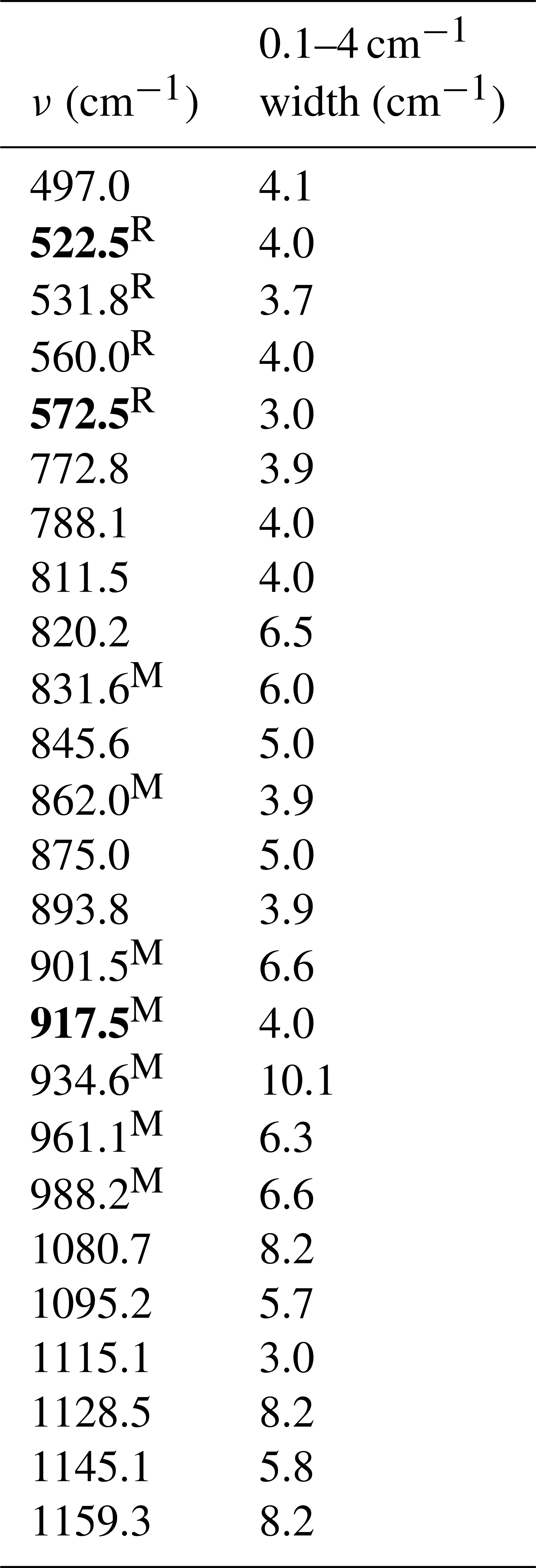
The optimal nonlinear inverse method iteratively retrieves cloud properties (COD, fice, rliq, and rice), using the results of the fast retrieval as a first guess. The inverse method uses radiances from 400 to 600 cm−1 (allowing thermodynamic phase determination; Rathke et al., 2002a) and from 750 to 1300 cm−1, which is sensitive to phase, COD, and effective radius. Similar optimal nonlinear inverse methods have been used to retrieve cloud properties from AERI instruments in the Arctic (Turner, 2005; Cox et al., 2014) and from satellite instruments (Wang et al., 2016; Poulsen et al., 2012; L'Ecuyer et al., 2019). Cloud properties are retrieved from observed radiances averaged in microwindows (see Table 2). The remainder of this section provides additional details about the optimal nonlinear inverse method.
Table 2Microwindows used in the optical and microphysical cloud property retrievals. The first column gives the central wavenumber, and the second column gives the microwindow width for resolutions of 0.1 to 4 cm−1. For resolutions of 8 cm−1, some microwindows were widened slightly so that there was at least one point in the microwindow (a few were narrowed so that there was only one point). Two sets of microwindows were used in this work: a combination of those used by Rathke and Fischer (2000) and Mahesh et al. (2001), indicated with superscripts R and M, and microwindows similar to those used by Turner (2005), consisting of all wavenumbers in plain font (e.g., not bold).
The inversion equation used here is the iterative Levenberg–Marquardt method (Rodgers, 2000, and references therein),
where x is the state vector, with a priori xa and covariance matrix Sa. The subscript i indicates the iteration number and R is the observation, with covariance matrix Se. F is the forward model (described below), and the kernel (K) is the Jacobian matrix, computed numerically by perturbing each state variable in turn and rerunning F.
The Levenberg–Marquardt formulation is a hybrid of the Gauss–Newton formulation and the method of steepest descent, with γ=0 defaulting to Gauss–Newton. As γ increases, Eq. (6) becomes more heavily weighted towards steepest descent and convergence slows. Choosing γ is difficult, as a large value of γ will slow the retrieval. Here we start with γ=0. Each time the current iteration causes the root-mean-square (rms) error between measurement and forward model result to increase in magnitude by more than 1 RU, or by more than double the current error, γ is increased (first to γ=1 and then) by a factor of 10; the retrieval is then repeated with the new γ. After increasing γ, if a subsequent iteration does not increase the rms error as described above, γ is decreased by a factor of 10. Iterations are repeated until γ<0.01 or the maximum allowed number of iterations is reached.
Error in the retrieved state variable is given by the covariance matrix
Note that this equation applies only when γ=0. We find that our criterion of γ<0.01 results in negligibly different retrievals than for γ=0. Convergence is tested using
(Rodgers, 2000), where n is the length of x.
In this work, the observation R is derived from the simulated spectra described in Sect. 2 by averaging radiances in microwindows between strong gaseous emission lines. Microwindows used in this work for resolutions of 0.1 to 4 cm−1 are shown in Table 2. They span 3–10 cm−1 and include at least one radiance (wavenumber spacing is equivalent to resolution). For retrievals at 8 and 20 cm−1, the closest measurement point to each central microwindow frequency was used. Using radiances in microwindows minimizes the contribution by gases, increasing sensitivity to cloud and reducing errors. However, due to the finite resolution, gas emission from outside the microwindow is convolved into radiances within the microwindow. For example, at a resolution of 0.1 cm−1, in a microwindow of 4 cm−1, the contribution from gaseous absorption lines outside the microwindow will be minimal. As resolution gets coarser, the gaseous absorption lines bordering the microwindow contribute more and more, potentially decreasing sensitivity and increasing errors.
The state vector x is composed of COD, ice fraction, log of the effective radius of liquid, and log of the effective radius of ice, so that n=4. For the a priori (xa), means of the values of x used to create the base set are used (Table 1). The covariance matrix Sa is assumed to be diagonal, with diagonal elements based on a standard deviation of about one-half the range of values; this is used rather than using the standard deviations given in Table 1 to weight the retrieval heavily toward the measurement rather than the a priori. The error covariance matrix for radiance (Se) is assumed to be diagonal with elements based on the model errors described in the next section and the measured and simulated radiance errors due to any imposed errors, added in quadrature. The first guess values (i=0) are determined from the fast cloud property retrieval. The maximum number of allowed iterations was set to 20 and the tolerance for convergence was set to d2<1. For convenience, the result of the forward model acting on the retrieved state vector is termed the retrieved radiance.
The forward model (F) is calculated by running DISORT with the state variables and with effective-resolution gaseous optical depths (described below). Other inputs to DISORT include the solar contribution, surface albedo, temperature profile, and the Legendre moments that describe the phase function, single-scatter albedo, and COD, which depend on the state variables and cloud height. DISORT is run with 16 streams. Single-scattering properties were the same as for the fast preliminary retrieval.
3.3 Resolution and model errors
In this work, DISORT was used for both simulating the observed radiances and for the forward model F. DISORT requires gaseous layer optical depths, which are calculated more accurately for observed radiances compared to those used in F. Gaseous layer optical depths computed by LBLRTM are at monochromatic or perfect resolution and a fine wavenumber spacing, and DISORT must be run for each wavenumber, after which the radiance must be convolved to instrument resolution. This was done to simulate the observations but is too computationally intensive for the iterative inverse retrieval (i.e., for F). Instead, we develop a novel method for producing effective-resolution gaseous layer optical depths (given in the Appendix) so that DISORT need only be run for each microwindow.
Model errors arising from these differences are shown in Fig. 1b, as box-and-whisker plots of model errors for cloudy-sky radiances at 0.5 cm−1 resolution, in microwindows used in the cloud optical and microphysical property retrievals. The errors were calculated as differences between downwelling radiances calculated using the effective-resolution layer optical depths (described in the Appendix) and monochromatic radiances convolved with the instrument line shape (the radiance simulations described in Sect. 2), and averaged in microwindows. At 0.5 cm−1 resolution, median model errors are within ±0.02 RU (1 RU = 1 mW/(m2 sr cm−1)). For resolutions of 0.1 to 2 cm−1, all model errors are within ±0.15 RU (figures for other resolutions are given in the Supplement). For resolutions of 4 to 20 cm−1, model errors generally increase with coarsening resolution, with maximum errors of −0.7 to 1.0 RU at 20 cm−1 resolution (Supplement).
Another source of model error is related to the cloud-height retrieval. The cloud-height retrieval also uses effective-resolution terms: the gaseous radiance and the transmittance from the surface up to each possible cloud layer (Rc and tc) and the clear-sky radiance (Rclr), described in Rowe et al. (2016). Derivation of these quantities is given in the Appendix. Model errors for a typical clear-sky radiance used in the cloud-height retrievals are also shown in Fig. 1b (solid blue curve); the error shown is the difference between Rclr calculated in this work (as described in the Appendix) and the monochromatic radiance from LBLRTM convolved with the instrument line shape. As the figure shows, model errors for clear skies are typically very low.
To determine the impact of sources of error on the cloud property retrievals, various errors were imposed on observed radiances, including Gaussian noise (mean of 0.2 RU) and bias (±0.2 RU). In remote locations, reanalysis datasets may be used for specification of the atmospheric state. Wesslen et al. (2014) characterized temperature errors in the European Centre for Medium-Range Forecasts (ECMWF) Interim (ERA-Interim; Dee et al., 2011) as varying from −0.5 to 1 K. Rowe et al. (2016) found such errors to have a roughly equivalent effect on radiative transfer calculations as a positive temperature bias of 0.2 K. Wesslen et al. (2014) characterized water vapor errors to be 2 % to 10 %, with lower biases in the first 3 km and higher biases above. Because water vapor decreases rapidly with height, this was found to be roughly equivalent to a water vapor bias at all heights of 3 % (Rowe et al., 2016). Thus, imposed errors also included biases in the atmospheric temperature (±0.2 K) and water vapor (±3 %). Higher biases in water vapor and temperature were also tested (±10 % and ±1 K). Cloud optical and microphysical properties were retrieved with these errors each imposed in isolation, using both true cloud heights and cloud heights retrieved with CO2 slicing as described in Rowe et al. (2016).
In addition to errors imposed in isolation, various combinations of the above sources of errors were imposed on retrievals, as described in Sect. 5 below.
5.1 Retrieval overview
Use of the fast retrieval as a starting point for the inverse retrieval was found to have a variety of benefits. The fast retrieval reduced rms errors relative to the a priori: from 300 % to 6 % for τg, from 0.4 to 0.2 for fice, from 4.4 to 3.7 µm for rliq, and from 16 to 11 µm for rice. This provided a first-guess for the inverse retrieval that was closer to the solution, lowering retrieval errors slightly, modestly increasing the number of cases that converged, and preventing convergence to an incorrect solution for a few cases. Overall, the greatest improvement from using the fast preliminary retrieval was reducing computation time; on average, one fewer iteration was needed when the fast retrieval was used.
Figure 2 shows the inverse-retrieval trajectory, with iterations, for an ice-only cloud with a COD of 0.89 and effective radius of 22 µm. The retrieval trajectory is superimposed on error contours (root-mean-square radiance differences). As the figure shows, the retrieval converged from the first-guess value (red dot on right in each panel), to the minimum in four iterations. Furthermore, the retrieval correctly converged to an ice-only cloud, although the mean cloud temperature of ∼256 K falls within the range of temperatures where mixed-phase clouds may occur.
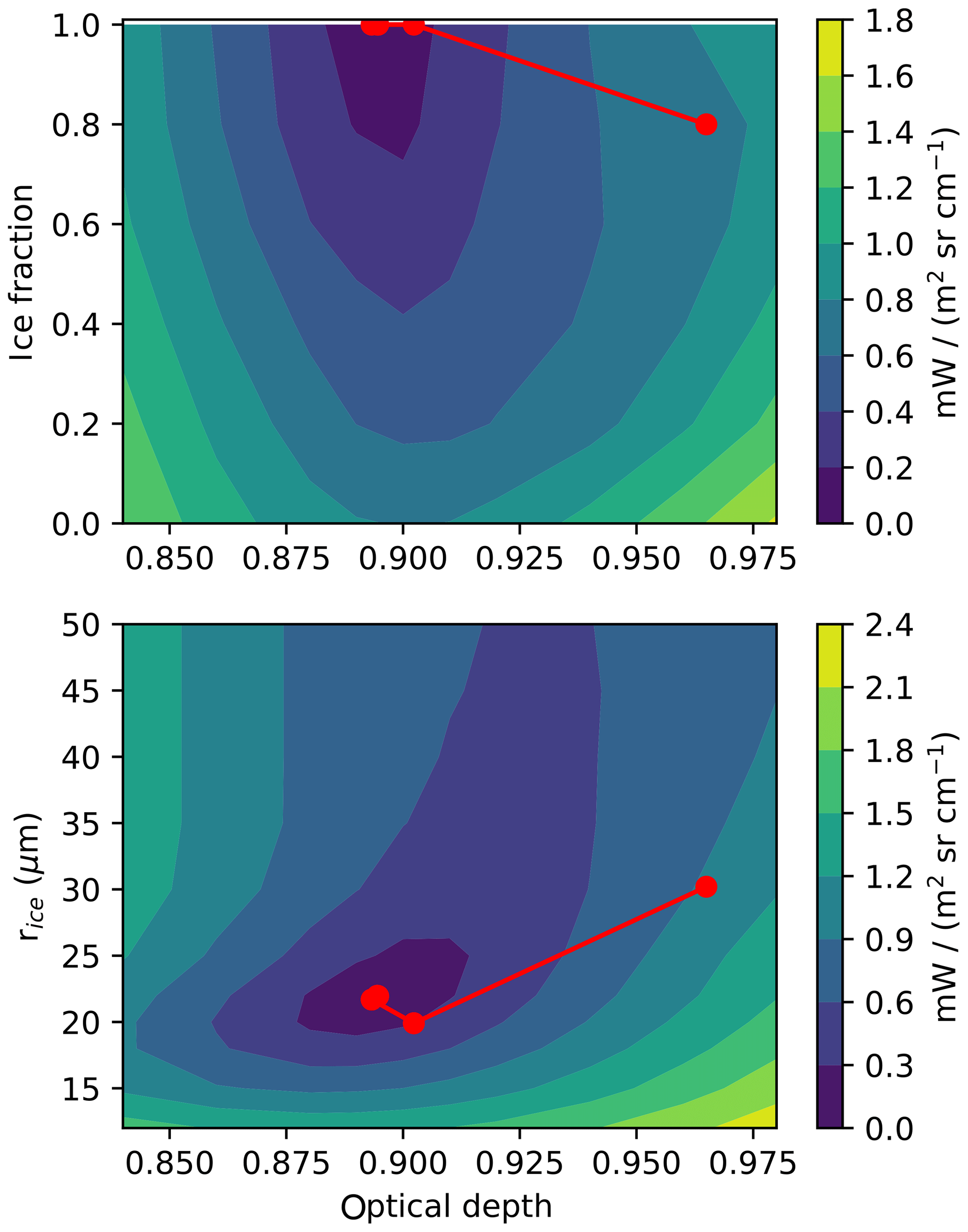
Figure 2Error contours for retrievals of ice effective radius (rice), ice fraction, and cloud optical depth, as root-mean-square error in radiances for an ice-only cloud. The retrieval trajectory (red line) and results for each iteration (red dots) are superimposed on the contour surface.
Retrievals using the base set of simulations indicate that the kernels are typically sufficiently linear to converge on the solution, except for large COD and effective radii. We find that the retrievals lose sensitivity to COD between about 5 and 10 (see Sect. 5.2 below); in previous work retrieving cloud properties from downwelling IR radiances in a similar wavenumber range, cutoffs of 4 to 6 were used (Mahesh et al., 2001; Rathke, 2002a, b; Turner, 2005). The retrievals were found to lose sensitivity to effective radius above about 50 µm (see Supplement), which is in keeping with Rathke and Fischer (2000) and Garrett and Zhao (2013), but differs from the cutoff values of 25 µm used by Mahesh et al. (2001) and of 100 µm by Turner (2005). In addition, when values approach these limits, the retrieval was found to sometimes move away from the solution. To avoid this, upper bounds were set for the COD (10) and effective radius (50 µm), and the kernels were typically calculated for a step in the direction of smaller COD and effective radius, that is, in the direction where sensitivity is larger.
Nearly all retrievals converged to within the specified tolerance in d2, with only zero to two cases failing to converge for any set of imposed errors. Overall, convergence was achieved in a mean of four iterations (median of three). At most two cases failed to converge within 20 iterations for any set of imposed errors.
5.2 Retrieval errors
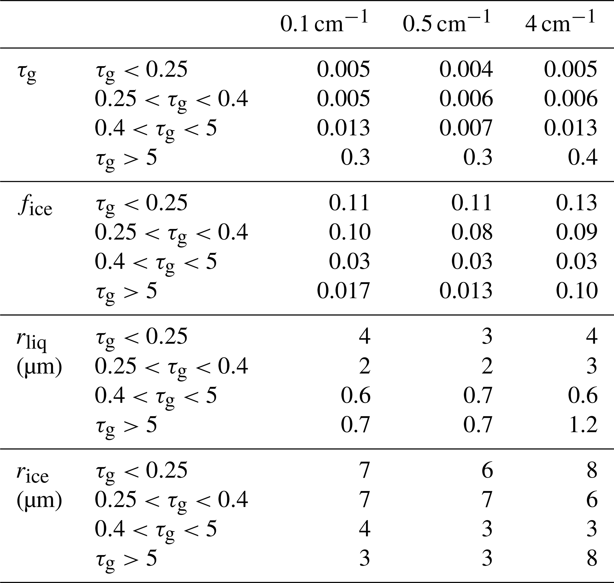
To determine the retrieval capability, errors in retrieved values are examined in the absence of any imposed errors, where only model errors are present. Table 3 shows errors in retrieved cloud properties (τg, fice, rliq, and rice) for the base set of spectra, for spectral resolutions of 0.1, 0.5, and 4 cm−1. Retrieval errors are shown for different ranges of τg. For thin clouds (τg < 0.4), the low signal reduces sensitivity. For thick clouds (τg > 5), the spectrum begins to approach saturation, and sensitivity to cloud optical and microphysical properties diminishes. Thus, both large and small τg values can result in large errors in fice, rliq, and rice (such increases are not seen for τg > 5 in Table 3 but occur when errors are imposed). By contrast, error in τg increases with increasing τg and is smallest for the thinnest clouds. Based on these considerations, the ideal range for τg was identified as 0.4 < τg < 5. (To get a sense of how common such clouds are, Cox et al. (2014) found that at Eureka, Nunavut, in 2006–2009, clouds with optical depths of 0.25 to 6 accounted for about 32 % of AERI measurements, 17 % when quality control procedures and a PWV threshold of 1 cm were applied; in this work PWV is as high as 3 cm.) Unless otherwise specified, results will be presented for this range. Retrieval errors for 0.4 < τg < 5 are overall quite low, with magnitudes of errors in τg below 0.013, in fice below 0.03, in rliq below 0.7 µm, and in rice below 4 µm. Overall, the table shows no trend in retrieval errors with coarsening resolution for 0.4 < τg < 5.
Table 3Root-mean-square errors in retrieved cloud properties for base set of spectra due to model error only (no errors imposed) for spectral resolutions indicated. Errors are shown for cloud geometric optical depth (τg), ice fraction (fice), effective radius of liquid (rliq), and effective radius of ice (rice) for four ranges in τg.
Retrieval accuracy was tested for two sets of microwindows. Set 1 consists of 22 microwindows similar to those used by Turner (2005), indicated in Table 2 in plain (non-bold) font; these were used in the retrievals described below. Set 2 consists of the combined microwindows of Rathke et al. (2000) and Mahesh et al. (2001), indicated in Table 2 with superscripts R and M (11 microwindows). Retrieval errors were found to be slightly lower for set 1; therefore it is used in the remainder of this work. However, differences were small (compare Table 4, described below, to Table S1 of the Supplement), indicating that a smaller set of microwindows is likely sufficient. Choice of optimal microwindows depends on noise level and spectrally varying errors (e.g., due to errors in assumed profiles of atmospheric water vapor and chlorofluorocarbons) and is therefore a complicated but interesting topic for future work.
Errors in retrieved cloud properties for different imposed errors are given in Table 4 for a spectral resolution of 0.5 cm−1 and τg between 0.4 and 5. Magnitudes of imposed errors are given in the first column except for cases of combined errors. Error combination (a) includes noise of 0.2 RU, radiation bias of 0.2 RU, temperature bias of 0.2 K, and water vapor bias of −3 %, and uses true cloud heights. Combination (b) is the same but with opposite signs on biases. Combinations (c) and (d) are the same as (a) and (b), respectively, but use retrieved cloud heights (similar sets but with radiation biases of 0.5 RU are given in Table S2 of the Supplement). Subsequent columns give the mean errors and the standard deviations of the errors.
Table 4Errors in retrieved cloud properties (mean error and standard deviation of error; SD; COD refers to cloud optical depth in the geometric limit, rliq and rice are the effective radii of liquid and ice) for various errors imposed on the observations (see text).
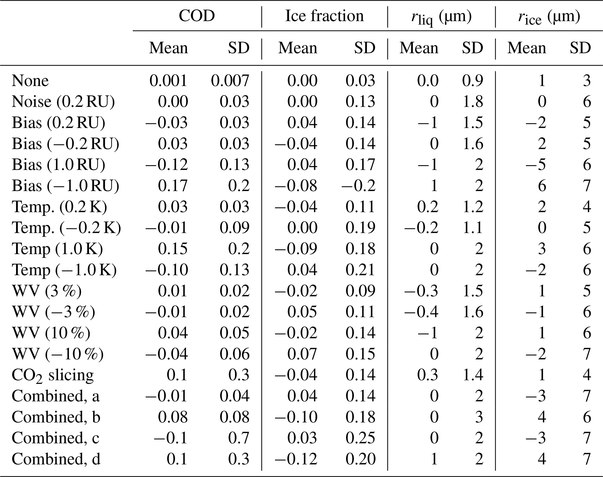
When true cloud heights are used, errors in τg are within ±0.2 for large biases imposed on the observed radiation, temperature, and water vapor, (±1.0 RU, 1 K, and 10 %, respectively) or combined errors, and within ±0.09 for smaller imposed biases (±0.2 RU, 0.2 K, and 3 %, respectively). Large imposed errors also lead to large errors in fice, making it difficult to distinguish liquid and ice. Errors in rice are typically 2 to 3 times larger than errors in rliq. Mean errors reveal how biases in measured radiance, water vapor, and temperature lead to biases in retrieved cloud properties. For example, positive biases in observed radiances lead to negative biases in COD, rliq, and rice, and positive biases in ice fraction, while the reverse is true for negative biases in observed radiance.
When cloud heights are retrieved from the observed radiances (columns labeled CO2 slicing and combined errors (c) and (d)), errors in cloud height lead to biases in inferred cloud temperature. Biases in cloud temperature cause errors that are spectrally flat. Because cloud emissivity depends fairly linearly on τg, spectrally flat errors have a large effect on τg. Furthermore, in the cloud-height retrieval (CHR), the cloud is placed in the atmospheric model layer containing the cloud height retrieved with CO2 slicing. This means that errors in COD are also affected by the choice of atmospheric layering. One approach to improving cloud temperature and optical depth is the geometric method of Rathke et al. (2002b), for which the instrument would be designed to look at multiple angles; this can also be used to examine the horizontal homogeneity of clouds.
Additional work is needed to understand the effects of CHR errors on cloud optical and microphysical property retrievals, for several reasons. First, Rowe et al. (2016) found that CHR errors for CO2 slicing were most sensitive to biases in observed radiance and temperature, with less sensitivity to noise and biases in water vapor. By contrast, for an alternate CHR method (MLEV) these sensitivities were found to be the opposite. Since CHR errors translate into errors in retrieved COD, it is important to choose the CHR method to use based on expected error magnitudes. Second, Rowe et al. (2016; see, e.g., Fig. 7) found that CHR errors generally decrease with increasing cloud signal, which should oppose the tendency of optical and microphysical property retrieval errors to grow with increasing COD. Finally, Rowe et al. (2016; Fig. 7) found that CHR errors generally decrease with decreasing cloud height. Here we find important consequences for retrievals of COD and fice. For example, when errors are imposed (noise of 0.2 RU, radiation bias of 0.2 RU, temperature bias of 0.2 K, water vapor bias of −3 %, and CHR errors in cloud height, for spectra at 4.0 cm−1 resolution), comparing clouds with bases above 2 km to those with bases below, rms errors in retrieved COD decrease from 1.1 to 0.15, errors in fice decrease from 0.3 to 0.18, and errors in rice decrease from 10 to 7 µm (errors remain at 2 µm for the effective radius of liquid).
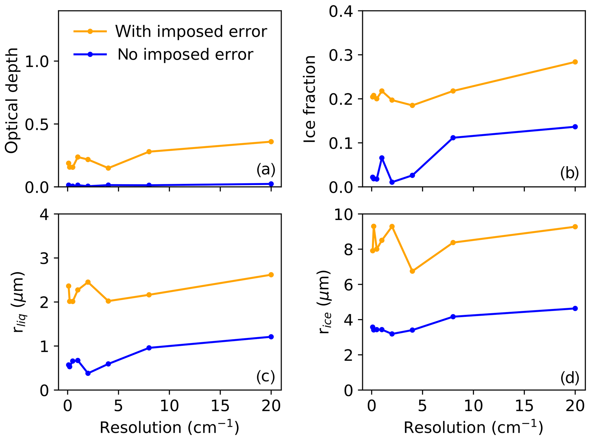
Figure 3Root-mean-square error in retrieved cloud properties as a function of resolution, where rliq is the effective radius of liquid and rice is the effective radius of ice, for cases with and without imposed error, as described in the text.
Errors in retrieved cloud properties are shown as a function of resolution from 0.1 to 20 cm−1 for clouds with bases below 2 km, in Fig. 3. Errors are shown for base cases with no imposed error and for a combination of imposed errors: noise of 0.2 RU, radiation bias of 0.2 RU, temperature bias of 0.2 K, water vapor bias of −3 %, and CHR errors in cloud height. No trend is seen in retrieval errors for resolutions of 0.1 to 4 cm−1, after which errors increase. For clouds with bases above 2 km, errors are larger for optical depth and ice fraction (Fig. S4 of the Supplement), and trends with resolution are similar but less pronounced. (Scatter plots of true vs. retrieved cloud properties are given in Figs. S5 and S6 of the Supplement.) Based on these trends, an instrument resolution of 4 cm−1 seems to be a good compromise for reducing resolution while avoiding increases in retrieval errors. For example, at 0.5 cm−1 (for clouds at all heights), rms retrieval errors are 0.6 for COD, 0.2 for fice, 3 µm for rliq, and 8 µm for rice; at 4 cm−1 they are nearly the same (0.6, 0.2, 2, and 8 µm, respectively).
5.3 Retrieval error covariance matrix
Discussion of errors so far has focused on actual retrieval errors, which can be calculated because simulated data were used as the observation set. For real measurements, error analysis relies on the covariance matrix S, which in turn depends on the kernels and covariance Se (Eq. 8); Se is calculated by adding measurement and forward model errors in quadrature; model errors are determined from errors in water vapor or temperature profiles. Here we determine how well S represents retrieval errors. For unbiased, normally distributed errors, the diagonals of S should correspond to the 68 % confidence interval. We can test this by comparing retrieval errors to the diagonal of S. This is complicated by the fact that S is not constant but depends on x (because the kernels depend on x). Thus for each retrieved x, the absolute error was divided by the square root of the appropriate diagonal element of the corresponding S. For Gaussian errors, this ratio should be < = 1 for 68 % of retrievals (and < = 2 for 95 % of retrievals). In the absence of imposed error, only 52 % to 63 % of retrievals had a ratio within 1 (for Se based on model errors). The lowest model errors are likely underestimates since it is unlikely all sources of error in the forward model were captured. A minor increase in model error (0.03 RU) gave values between 68 % and 77 %. However, the error distributions were found to decrease more slowly than Gaussians, with only 78 % to 87 % of errors (rather than 94 %) falling within the second standard deviation indicated by S.
For imposed noise of 0.2 RU, only 52 % to 58 % of retrievals were found to have a ratio within 1, suggesting that model errors are amplified in the presence of error. This is likely because away from the correct solution, the estimate of S is incorrect. Increasing the contribution of noise to Se by 30 % accounted for this, resulting in values of 65 % to 70 %.
S was found to provide a poor indication of retrieval errors due to biases in radiance, temperature, water vapor, or cloud height. This is likely because the inverse retrieval is based on an assumption of unbiased, normally distributed errors. For biases in radiance and water vapor and for errors in cloud height, S is particularly nonrepresentative for COD, for which only 11 % to 25 % of cases fall within 1 standard deviation for S (for other properties the range is 36 % to 78 %). Biases in temperature affect S similarly for COD, fice, rliq, and rice (range of 48 % to 66 %). This underscores the importance of removing bias errors from measurements whenever possible to ensure that S provides the best possible representation of errors.
5.4 Cloud vertical inhomogeneity and ice habit
Errors in retrieved cloud properties (from spectra at 0.5 cm−1 resolution) due to failing to capture cloud vertical inhomogeneity are shown in Table 5. For the upper set of cases shown in the table, errors were not imposed and true cloud heights were used. In performing the retrieval the correct cloud base and top were used, but the cloud was assumed to be vertically homogeneous in terms of COD and phase; thus the cloud model is accurate for dense and diffuse clouds but not for inhomogeneous or liquid-topped clouds. This emulates a measurement where the cloud base and top are known from an ancillary instrument such as a lidar. As expected, therefore, errors are similar for dense and diffuse clouds. For inhomogeneous clouds, which are thinner at the upper and lower edges, errors are slightly larger for τg. The largest retrieval errors are found to be for liquid-topped clouds, particularly for τg and fice, for which errors are about 5 times as large. These errors are large because the cloud heights are effectively wrong for the liquid and ice layers of the cloud. A lidar that can classify phase would allow reduction of these errors down to the level seen for other cloud types. The enhancement of errors in liquid-topped clouds relative to other cloud types disappears when errors are imposed on the observations (imposed noise of 0.2 RU, radiation bias of 0.2 RU, temperature bias of 0.2 K, and water vapor bias of −3 %; see the last two sets of cases in Table 5). This is true when true cloud heights are used (middle set) and when they are retrieved (lowest set). (Similar trends are found when the radiation bias is increased to 0.5 RU, as shown in the Supplement.)

Figure 4Radiance errors (1 RU = 1 mW/(m2 sr cm−1)) for different methods of approximating the radiance at a resolution of 0.5 cm−1. Approximate radiances are computed using mean perfect-resolution layer optical depths , mean surface-to-layer perfect-resolution transmittances , or mean surface-to-layer transmittances after convolution to the instrument R(〈t〉); averages are over 0.5 cm−1 (a) or over microwindows (b). Approximate radiances are compared to simulated radiances at 0.5 cm−1 resolution (Rclr), which are averaged over microwindows in (b).
Table 5Root-mean-square errors in retrieved cloud properties for vertically varying clouds: cloud optical depth (COD), ice fraction (fice), and effective radii of liquid and ice (rliq and rice). For the upper set of cases, errors were not imposed on observations (error =n) and true cloud heights were used. The middle set of cases includes imposed errors with true cloud heights (error =y), while the lowest set includes imposed errors with retrieved cloud heights (error ; see text).
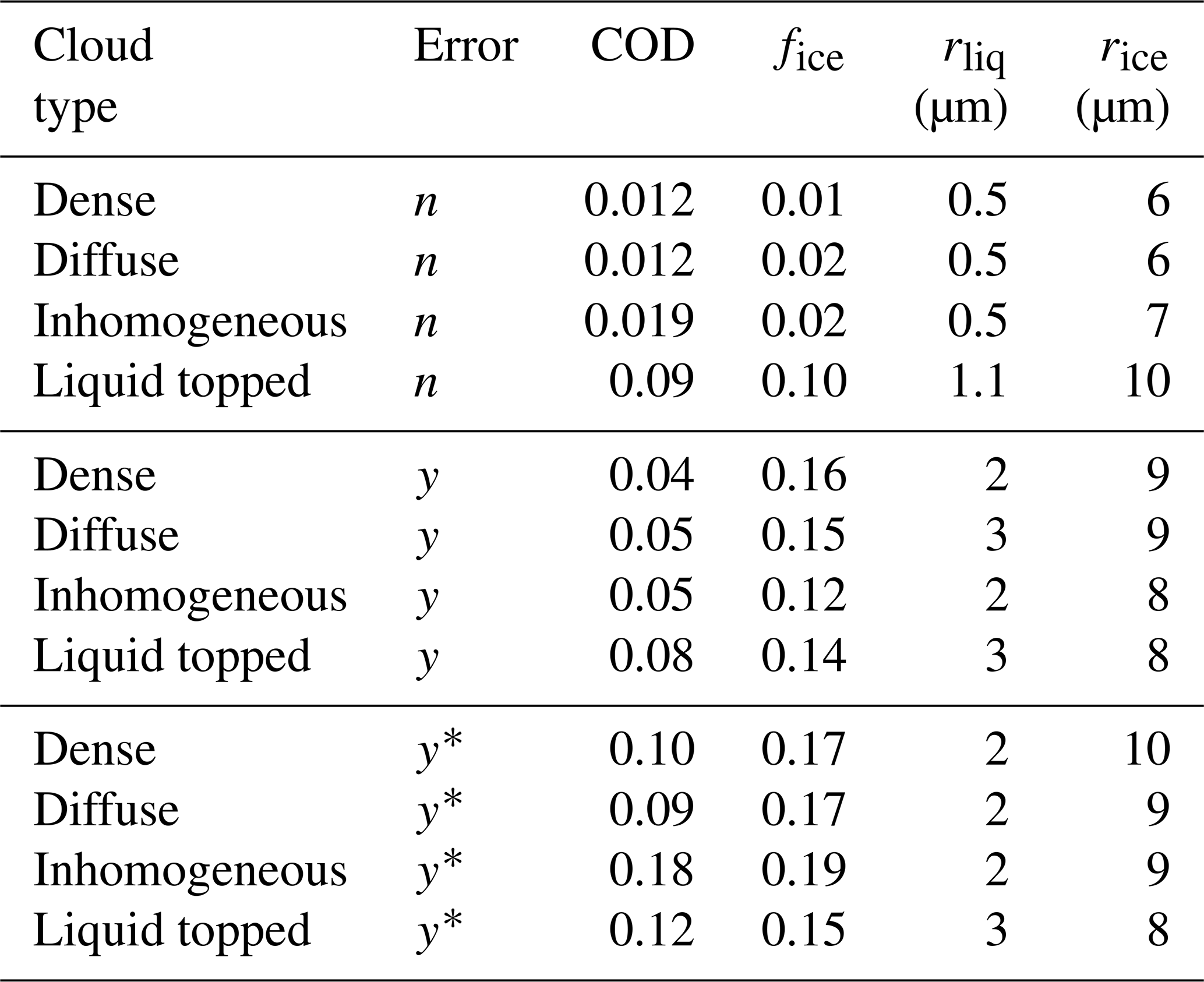
Table 6Root-mean-square errors in retrieved cloud properties, assuming a spherical ice habit, for ice clouds of varying habit (first column): cloud optical depth (COD), ice fraction (fice), and effective radius of ice (rice). For the upper set of cases, errors were not imposed (error =n) and true cloud heights were used. The middle set of cases includes imposed error with true cloud heights (error =y), while the lowest set includes imposed errors with retrieved cloud heights (error ; see text).
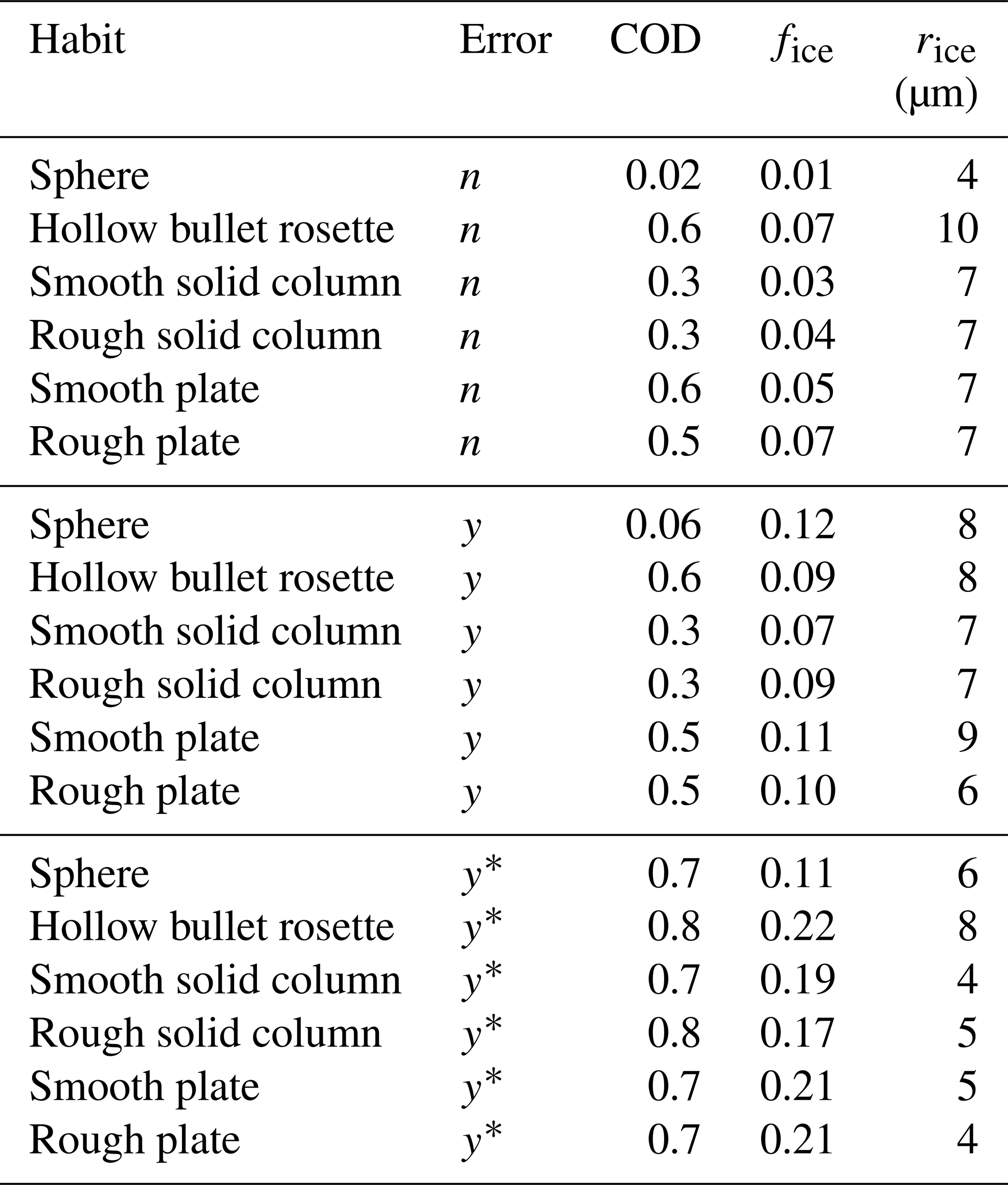
Errors in retrieved cloud properties (from spectra at 0.5 cm−1 resolution) due to assuming a spherical ice habit are shown in Table 6. The first column of the table shows the true ice habit. The upper set of data has no other imposed errors, while the lower two sets have the same imposed errors as for vertically varying clouds. Retrieval error in rliq is not shown because clouds were mainly ice. In the absence of imposed errors, compared to spheres, the increase in error is greatest for τg, for which errors increase by an order of magnitude or more. This large increase suggests that errors in habit mainly bias the magnitude rather than spectral shape of the cloud emissivity. Overall, errors are the smallest for solid columns. However, differences in errors based on assumed ice habit diminish when errors exist in observations and cloud heights are retrieved (bottom set). Thus, using a realistic ice habit can minimize errors, but this becomes less important when cloud height is also retrieved.
This work explores the capability of a low-resolution IR spectrometer for retrieving cloud properties in polar regions. To this end, the CLoud and Atmospheric Radiation Retrieval Algorithm (CLARRA) was used to retrieve cloud properties (height, following Rowe et al., 2016, as well as COD, ice fraction, effective radius of liquid, and effective radius of ice) from simulations of surface-based IR downwelling radiances, to determine the effect of instrument resolution on accuracy. CLARRA includes a method for calculating gaseous transmission and emission terms at the effective instrument resolution, minimizing model errors. A fast-forward retrieval rapidly retrieves preliminary cloud optical and microphysical properties, which then serve as inputs into an optimal nonlinear inverse method. Cloud properties were retrieved from 222 simulated radiances based on atmospheric and cloud conditions characteristic of the Arctic, with additional tests of sensitivity to cloud vertical inhomogeneity and ice habit.
Sensitivity studies for vertically varying clouds indicate that, in the absence of observational errors, errors in retrieved cloud properties are highest for liquid-topped clouds that are assumed to be homogeneously mixed phase (relative to clouds that are dense, diffuse, or inhomogeneous vertically). However, in the presence of errors in observations, the gap in retrieved cloud-property errors between liquid-topped clouds and other cloud structures disappears. Future work is needed to assess errors when multiple cloud layers are present. For different ice habits, sensitivity studies indicate that use of a reasonable guess for the ice habit can help minimize errors, but these differences become minor in the presence of observational errors.
Retrieval accuracy was determined as a function of resolution for model errors, CHR errors, and a variety of imposed observational errors, including random noise as well as biases in the measured spectrum and atmospheric state. In the absence of imposed errors, errors in retrieved cloud properties were found to be 0.007 for COD, 0.03 for fice, 0.7 for rliq, and 3 µm for rice (0.5 cm−1 resolution; COD between 0.4 and 5). In the presence of imposed errors, errors in retrieved COD and ice fraction were found to be strongly affected by bias errors in cloud height, which in turn are high when the CHR is used. Furthermore, CHR errors typically decrease with decreasing cloud base height (Rowe et al., 2016), with consequences for optical and microphysical property retrievals. For example, for a combination of errors including noise of 0.2 RU, radiation bias of 0.2 RU, temperature bias of 2 K, water vapor bias of −3 %, and CHR errors (at 4.0 cm−1 resolution), comparing clouds with bases above 2 km to those with bases below, the rms error decreases from 1.1 to 0.15 for COD and from 0.3 to 0.18 for fice, pointing to a strong potential for retrievals of low clouds.
Retrieval errors were found to be fairly invariant to resolution up to about 4 cm−1, after which accuracy declined. For example, at 0.5 cm−1 resolution, for the combination of errors given above, rms retrieval errors (for clouds at all heights) are 0.7 for COD, 0.2 for fice, 3 µm for rliq, and 8 µm for rice. At 4 cm−1 these errors are similar (0.6, 0.2, 2, and 8, respectively). Taken together, this lack of sensitivity to resolution indicates that a moderately low-resolution (∼4 cm−1) surface-based IR spectrometer could provide cloud property retrievals with accuracy comparable to existing higher-resolution instruments. Furthermore, these retrievals would be particularly useful for low-level clouds, for which accuracy is likely to be highest.
Simulated radiances at monochromatic resolution (Cox et al., 2015) are available by email to the corresponding author. Computer code is available at Bitbucket (https://bitbucket.org/{4e9c3a2c-5ac5-40f9-a7e4-0c9578f88b21}, Rowe, 2019), including repositories containing Python computer code (runDisort_py) and MATLAB/Octave computer code (runDisort_mat) for creating cloudy-sky spectra using DISORT (Stamnes et al., 1988). See also Rowe et al. (2013, 2016).
To solve the radiative transfer equation in LBLRTM and DISORT (Stamnes et al., 1988), the atmosphere is divided into model atmospheric layers and the approximation is made that the Planck function varies linearly with optical depth through the layer (Wiscombe et al., 1976; Clough et al., 1992). In the absence of scattering, the downwelling radiance from a layer at a given wavenumber is approximated as
where the tildes indicate monochromatic, or perfect, resolution (all quantities with tildes depend on wavenumber), τ is defined as the vertical optical depth from the surface up to some height (e.g., within layer L), τL−1 is from the surface to the layer bottom, and τL is from the surface to the layer top. (Parentheses are used here and below to indicate dependence.) is the Planck function and θ is the viewing angle from zenith. Note that the formulation here differs from that of Clough et al. (1992); here, RL, τL, and the transmittance, tL (defined below) are defined from the bottom of the model atmosphere (e.g., from Earth's surface) to the top of layer L. Quantities that are for layer bottom to top only are indicated with a delta. Using these conventions means that Eq. (A1) represents the radiance from layer L that is transmitted by the atmosphere below to the surface. The viewing angle is included explicitly here so that τ refers to the vertical optical depth.
The surface-to-layer-top transmittance depends on the optical depth,
The linear-in-optical depth approximation for B allows the integral to be solved, yielding
where and are the Planck functions of the temperature at the lower and upper boundaries of layer L, and the deltas indicate the change across the layer. (Note that is calculated slightly differently in LBLRTM, following Clough et al., 1992; the two methods give similar results.)
Thus ΔRL is the radiance from the layer that makes it to the surface. The total (clear-sky) radiance is the sum of all the layer radiances. To match instrument resolution, the clear-sky radiance needs to be convolved with the instrument line shape S,
where the dependence on wavenumber has been included explicitly. Equation (A4) can also be calculated directly by running LBLRTM and convolving with the S (typically a sinc function). We will use Rclr calculated in this manner to test the remaining approximations.
In practice the integral need only be performed over the small wavenumber region characterized by the width of S (typically a sinc function). Switching the order of the sum and the integral, we have
where
In addition to Rclr, the cloud-height retrieval (Rowe et al., 2016) requires the gaseous radiance from the surface up to each possible cloud layer (Rc), which can also be calculated from ΔRL,
Finally, the cloud-height retrieval requires the transmittance of the atmosphere below the cloud (tL; in Rowe et al., 2016, it is referred to as tc) at the effective instrument resolution. Examining Eqs. (A1)–(A6) shows that it is more accurate to convolve the Planck function multiplied by the surface-to-layer transmittance. Thus we define the effective transmittance from the surface to a layer as
To summarize how these approximations are used for the cloud-height retrieval, first gaseous layer optical depths are computed using LBLRTM. Next, values are summed from the surface up to each layer to get . Equation (A2) is then used to calculate , and Eqs. (A3) and (A6) are used to calculate ΔRL. Equation (A5) is used to calculate Rclr, and Eq. (A7) is used to calculate Rc for each model layer that could contain cloud (for cloud heights within layers, terms are interpolated). Equation (A8) is used to calculate tL.
A1 Approximations and model error for cloud optical and microphysical property retrievals
Retrieval of optical and microphysical cloud properties requires effective-resolution layer optical depths, ΔτL, as input into the DISORT radiative transfer code. One method to create the set of ΔτL might be to reduce the resolution of the layer optical depths. However, the above equations suggest that a more accurate method would be in terms of transmittances. Inserting Eq. (A2) into Eq. (A8) and breaking up the integral gives
The first two terms on the right-hand side of this equation have the same form as the integral in Eq. (A8) and can be replaced with −BLtL and . Thus it makes sense to create the set of ΔτL using tL (noting that the third term in Eq. A9 also includes the monochromatic layer gaseous optical depth and thus represents a source of error).
Due to ringing, tL can be greater than 1 or less than 0, resulting in optical depths outside physical bounds. To minimize ringing, transmittances were averaged over small spectral regions between strong emission lines, or microwindows (Table 2). Observed radiances are therefore also averaged over microwindows. (Note that it might be more accurate to average the term in brackets in Eq. A8; an alternate option would be to use an apodization function rather than a sinc function in Eq. A8 to reduce ringing; these are both interesting topics for future work.) Following this, transmittances below 10−40 and above 1 were modified such that 10.
Finally, layer optical depths are calculated from tL. For the first layer,
For subsequent layers, the optical depths of all layers below must be subtracted.
The advantage of approximating radiances using layer optical depths derived from surface-to-layer transmittances convolved to the instrument resolution is shown in Fig. 4. Errors for this convolved-transmittance (CT) method are compared to errors for radiances calculated using optical depths derived from averaged monochromatic surface-to-layer transmittances (or from averaged monochromatic layer optical depths). In Fig. 4a averages are over the wavenumber spacing (no averaging is needed for the CT method, for which the spectra are already at the appropriate wavenumber spacing). Figure 4b shows errors for averages over microwindows. Errors are determined by comparison with Rclr calculated as in Eq. (A4), using LBLRTM and then convolving to the desired resolution (0.5 cm−1 here) and (in b) averaged over microwindows. Errors are reduced significantly by the CT method, relative to the other approximations. In microwindows (Fig. 4b), errors are within 3 or 30 RU for the other methods, whereas for the CT method they are (for this example, the range for cloudy cases used in this work is shown in Fig. 1); thus the CT method represents a significant improvement. Finally, it is worth noting that errors at instrument resolution are also fairly low (Fig. 4a). This is shown here for reference only, and is not used in this work, but has the potential for use in a cloud-height retrieval that includes scattering, using DISORT.
To summarize the approximations used for the cloud optical and microphysical property retrievals, the set of effective-resolution gaseous layer optical depths needed for running DISORT is calculated as follows. The first few steps are the same as for the cloud-height retrieval: values are computed using LBLRTM and these are summed from the surface to each layer to get , and Eq. (A2) is used to calculate . Next, Eq. (A8) is used to calculate tL, which is then averaged over microwindows and bounded to be between 10−40 and 1. Equations (A10) and (A11) are then used to calculate ΔτL. Since DISORT is run at single precision, serious errors can result for very small input optical depths; thus ΔτL was increased as needed such that .
The supplement related to this article is available online at: https://doi.org/10.5194/amt-12-5071-2019-supplement.
SN calculated Legendre moments and single-scatter albedo from single-scattering parameters. CC led creation of simulated spectra used in this work. VPW conceived of the idea and provided guidance. PR performed all other calculations and wrote the paper with input from all authors.
The authors declare that they have no conflict of interest.
Computer code was written in the Python computing language and figures were created using Matplotlib. We are grateful for help with Python coding from Daniel Neshyba-Rowe and for advice on running DISORT from Istvan Laszlo.
This research has been supported by the National Science Foundation, Division of Arctic Sciences (grant no. 1108451), the National Science Foundation, Office of Polar Programs (grant no. 1543236), and the National Science Foundation, Division of Chemistry (grant no. 1807898).
This paper was edited by Andrew Sayer and reviewed by Bryan A. Baum and D. D. Turner.
Boucher, O., Randall, D., Artaxo, P., Bretherton, C., Feingold, G., Forster, P., Kerminen, V.-M., Kondo, Y., Liao, H., Lohmann, U., Rasch, P., Satheesh, S. K., Sherwood, S., Stevens, B. and Zhang, X. Y.: Clouds and Aerosols, in: Climate Change 2013: The Physical Science Basis. Contribution of Working Group I to the Fifth Assessment Report of the Intergovernmental Panel on Climate Change, edited by: Stocker, T. F., Qin, D., Plattner, G.-K., Tignor, M., Allen, S. K., Boschung, J., Nauels, A., Xia, Y., Bex, V. and Midgley, P. M., Cambridge University Press, Cambridge, United Kingdom and New York, NY, USA, 2013.
Bromwich, D. H., Nicolas, J. P., Hines, K. M., Kay, J. E., Key, E. L., Lazzara, M. A., Lubin, D., McFarquhar, G. M., Gorodetskaya, I. V., Grosvenor, D. P., and Lachlan‐Cope, T.: Tropospheric clouds in Antarctica, Rev. Geophys., 50, RG1004, https://doi.org/10.1029/2011RG000363, 2012.
Clough, S., Iacono, M. J., and Moncet, J. L.: Line-by-line calculations of atmospheric fluxes and cooling rates: Application to water vapour, J. Geophys. Res.-Atmos., 97, 15761–15785, 1992.
Clough, S., Shephard, M. W., Shephard, M. W., Mlawer, E. J., Delamere, J. S., Iacono, M. J., Cady-Pereira, K., Boukabara, S., and Brown, P. D.: Atmospheric radiative transfer modeling: a summary of the AER codes, J. Quant. Spectrosc. Ra., 91, 233–244, https://doi.org/10.1016/j.jqsrt.2004.05.058, 2005.
Cox, C., Turner, D. D., Rowe, P. M., Shupe, M., and Walden, V. P.: Cloud Microphysical Properties Retrieved from Downwelling Infrared Radiance Measurements Made at Eureka, Nunavut, Canada (2006–09), J. Appl. Meteorol. Climatol., 53, 772–791, https://doi.org/10.1175/JAMC-D-13-0113.1, 2014
Cox, C., Walden, V. P., Rowe, P. M., and Shupe, M.: Humidity trends imply increased sensitivity to clouds in a warming Arctic, Nat. Commun., 6, 10117, https://doi.org/10.1038/ncomms10117, 2015.
Cox, C. J., Rowe, P. M., Neshyba, S. P., and Walden, V. P.: A synthetic data set of high-spectral-resolution infrared spectra for the Arctic atmosphere, Earth Syst. Sci. Data, 8, 199–211, https://doi.org/10.5194/essd-8-199-2016, 2016.
Dee, D. P., Uppala, S. M., Simmons, A. J., Berrisford, P., Poli, P., Kobayashi, S., Andrae, U., Balmaseda, M. A., Balsamo, G., Bauer, P., Bechtold, P., Beljaars, A. C., van de Berg, L., Bidlot, J., Bormann, N., Delsol, C., Dragani, R., Fuentes, M., Geer, A. J., Haimberger, L., Healy, S. B., Hersbach, H., Hólm, E. V., Isaksen, L., Kållberg, P., Köhler, M., Matricardi, M., McNally, A. P., Monge-Sanz, B. M., Morcrette, J., Park, B., Peubey, C., de Rosnay, P., Tavolato, C., Thépaut, J., and Vitart, F.: The ERA-Interim reanalysis: configuration and performance of the data assimilation system, Q. J. Roy. Meteor. Soc., 137, 553–597, https://doi.org/10.1002/qj.828, 2011.
Francis, J. A. and Hunter, E.: New insight into the disappearing Arctic sea ice, Eos Trans. AGU, 87, 509–511, https://doi.org/10.1029/2006EO460001, 2006.
Garrett, T. J. and Zhao, C.: Ground-based remote sensing of thin clouds in the Arctic, Atmos. Meas. Tech., 6, 1227–1243, https://doi.org/10.5194/amt-6-1227-2013, 2013.
Hines, K. M., Bromwich, D. H., Rasch, P., and Iacono, M. J.: Antarctic Clouds and Radiation within the NCAR Climate Models, J. Climate, 17, 1198–1212, 2004.
Kay, J. E. and Gettelman, A.: Cloud influence on and response to seasonal Arctic sea ice loss, J. Geophys. Res., 114, D18204, https://doi.org/10.1029/2009JD011773, 2009.
Komurcu, M., Storelvmo, T., Tan, I., Lohmann, U., Yun, Y., Penner, J. E., Wang, Y., Liu, X., and Takemura, T.: Intercomparison of the cloud water phase among global climate models, J. Geophys. Res.-Atmos., 119, 3372–3400, https://doi.org/10.1002/2013JD021119, 2014.
Lachlan-Cope, T., Listowski, C., and O'Shea, S.: The microphysics of clouds over the Antarctic Peninsula – Part 1: Observations, Atmos. Chem. Phys., 16, 15605–15617, https://doi.org/10.5194/acp-16-15605-2016, 2016.
Lawson, R. P. and Gettelman, A.: Impact of Antarctic clouds on climate, Proc. Natl. Acad. Sci. USA, 111, 18156–18161, https://doi.org/10.1073/pnas.1418197111, 2014.
L'Ecuyer T. S. and Jiang J. H.: Touring the atmosphere aboard the A-Train, Phys. Today, 63, 36, https://doi.org/10.1063/1.3463626, 2010.
L'Ecuyer, T. S., Hang, Y., Matus, A. V., and Wang, Z.: Reassessing the effect of cloud type on Earth's energy balance in the age of active spaceborne observations, Part I: Top-of-atmosphere and surface, J. Climate, 32, 6197–6217, https://doi.org/10.1175/JCLI-D-18-0753.1, 2019.
Mahesh, A., Walden, V. P., and Warren, S. G.: Ground-based infrared remote sensing of cloud properties over the Antarctic Plateau, Part II: Cloud optical depths and particle sizes, J. Appl. Meteorol., 40, 1279–1294, 2001.
Palchetti, L., Bianchini, G., Di Natale, G., and Del Guasta, M.: Far-Infrared Radiative Properties of Water Vapour and Clouds in Antarctica, Bull. Am. Meteor. Soc., 96, 1505–1518, https://doi.org/10.1175/BAMS-D-13-00286.1, 2015.
Poulsen, C. A., Siddans, R., Thomas, G. E., Sayer, A. M., Grainger, R. G., Campmany, E., Dean, S. M., Arnold, C., and Watts, P. D.: Cloud retrievals from satellite data using optimal estimation: evaluation and application to ATSR, Atmos. Meas. Tech., 5, 1889–1910, https://doi.org/10.5194/amt-5-1889-2012, 2012.
Rathke, C. and Fischer, J.: Retrieval of Cloud Microphysical Properties from Thermal Infrared Observations by a Fast Iterative Radiance Fitting Method, J. Atmos. Ocean. Tech., 17, 1509–1524, https://doi.org/10.1175/1520-0426(2000)017<1509:ROCMPF>2.0.CO;2, 2000.
Rathke, C., Fischer, J., Neshyba, S., and Shupe, M.: Improving IR cloud phase determination with 20 microns spectral observations, Geophys. Res. Lett., 29, 1–4, https://doi.org/10.1029/2001GL014594, 2002a.
Rathke, C., Neshyba, S., Shupe, M., Rowe, P., and Rivers, A.: Radiative and microphysical properties of Arctic stratus clouds from multiangle downwelling infrared radiances, J. Geophys. Res., 107, 1–13, 2002b.
Rodgers, C. D.: Inverse methods for atmospheric sounding: theory and practice, Vol. 2., World Scientific, Singapore, 2000.
Rowe, P. M.: Computer code for the CLoud and Atmospheric Radiation Retrieval Algorithm (CLARRA), https://bitbucket.org/clarragroup/, last access: 13 September 13, 2019.
Rowe, P. M., Miloshevich, L. M., Turner, D. D., and Walden, V. P.: Dry Bias in Vaisala RS90 Radiosonde Humidity Profiles over Antarctica, J. Atmos. Ocean. Tech., 25, 1529–1541, https://doi.org/10.1175/2008JTECHA1009.1, 2008.
Rowe, P. M., Neshyba, S., and Walden, V. P.: Radiative consequences of low-temperature infrared refractive indices for supercooled water clouds, Atmos. Chem. Phys., 13, 11925–11933, https://doi.org/10.5194/acp-13-11925-2013, 2013.
Rowe, P. M., Cox, C. J., and Walden, V. P.: Toward autonomous surface-based infrared remote sensing of polar clouds: cloud-height retrievals, Atmos. Meas. Tech., 9, 3641–3659, https://doi.org/10.5194/amt-9-3641-2016, 2016.
Silber, I., Verlinde, J., Eloranta, E. W., and Cadeddu, M.: Antarctic cloud macrophysical, thermodynamic phase, and atmospheric inversion coupling properties at McMurdo Station: I, Principal data processing and climatology, J. Geophys. Res.-Atmos., 123, 6099–6121, https://doi.org/10.1029/2018JD028279, 2018.
Stamnes, K., Tsay, S.-C., Wiscombe, W. J., and Jayaweera, K.: Numerically stable algorithm for discrete-ordinate-method radiative transfer in multiple scattering and emitting layered media, Appl. Opt., 27, 2502–2509, https://doi.org/10.1364/AO.27.002502, 1988.
Turner, D. D.: Arctic mixed-phase cloud properties from AERI lidar observations: Algorithm and results from SHEBA, J. Appl. Meteorol., 44, 427–444, 2005.
Uttal, T., Starkweather, S., Drummond, J. R., Vihma, T., Makshtas, A. P., Darby, L. S., Burkhart, J. F., Cox, C. J., Schmeisser, L. N., Haiden, T., and Maturilli, M.: International Arctic Systems for Observing the Atmosphere (IASOA): An International Polar Year Legacy Consortium, Bull. Am. Meteor. Soc., 97, 1033–1056 https://doi.org/10.1175/BAMS-D-14-00145.1, 2015.
van den Broeke, M., Box, J., Fettweis, X., Hanna, E., Noël, B., Tedesco, M., As, D., van de Berg, W. J., and van Kampenhout, L.: Greenland Ice Sheet Surface Mass Loss: Recent Developments in Observation and Modeling, Current Climate Change Reports, 3, 345–356, https://doi.org/10.1007/s40641-017-0084-8, 2017.
Wagner, R., Benz, S., Möhler, O., Saathoff, H., Schnaiter, M., and Schurath, U.: Mid-infrared Extinction Spectra and Optical Constants of Supercooled Water Droplets, J. Phys. Chem. A, 109, 7099–7112, https://doi.org/10.1021/jp051942z, 2005.
Walden, V. P., Town, M. S., Halter, B., and Storey, J.: First measurements of the infrared sky brightness at Dome C, Antarctica, Publ. Astron. Soc. Pac., 117, 300–308, https://doi.org/10.1086/427988, 2005.
Wang, C., Platnick, S., Zhang, Z., Meyer, K., and Yang, P.: Retrieval of ice cloud properties using an optimal estimation algorithm and MODIS infrared observations: 1, Forward model, error analysis, and information content, J. Geophys. Res.-Atmos., 121, 5809–5826, https://doi.org/10.1002/2015JD024526, 2016.
Wang, X. and Key, J. R.: Arctic Surface, Cloud, and Radiation Properties Based on the AVHRR Polar Pathfinder Dataset, Part II: Recent Trends, J. Climate, 18, 2575–2593, https://doi.org/10.1175/JCLI3439.1, 2005.
Wang, Y., Yuan, X., Bi, H., Liang, Y., Huang, H., Zhang, Z., and Liu, Y.: The contributions of winter cloud anomalies in 2011 to the summer sea-ice rebound in 2012 in the Antarctic, J. Geophys. Res.-Atmos., 124, 3435–3447, https://doi.org/10.1029/2018JD029435, 2019.
Warren, S. G. and Brandt, R. E.: Optical constants of ice from the ultraviolet to the microwave: A revised compilation, J. Geophys. Res., 113, D14220, https://doi.org/10.1029/2007JD009744, 2008.
Wesslén, C., Tjernström, M., Bromwich, D. H., de Boer, G., Ekman, A. M. L., Bai, L.-S., and Wang, S.-H.: The Arctic summer atmosphere: an evaluation of reanalyses using ASCOS data, Atmos. Chem. Phys., 14, 2605–2624, https://doi.org/10.5194/acp-14-2605-2014, 2014.
Winker, D., Chepfer, H., Noel, V., and Cai, X.: Observational Constraints on Cloud Feedbacks: The Role of Active Satellite Sensors, Surv. Geophys., 38, 1483, https://doi.org/10.1007/s10712-017-9452-0, 2017.
Wiscombe, W. J.: Extension of the doubling method to inhomogeneous sources, J. Quant. Sprectrosc. Ra., 16, 477–489, 1976.
Yang, P., Bi, L., Baum, B. A., Liou, K. N., Kattawar, G. W., Mishchenko, M. I., and Cole, B.: Spectrally Consistent Scattering, Absorption, and Polarization Properties of Atmospheric Ice Crystals at Wavelengths from 0.2 to 100 µm, J. Atmos. Sci., 70, 330–347, https://doi.org/10.1175/JAS-D-12-039.1, 2013.
Zasetsky, A. Y., Khalizov, A. F., Earle, M. E., Sloan, J. J., and Sloan, J. J.: Frequency Dependent Complex Refractive Indices of Supercooled Liquid Water and Ice Determined from Aerosol Extinction Spectra, J. Phys. Chem. A, 109, 2760–2764, https://doi.org/10.1021/jp044823c, 2005.
- Abstract
- Introduction
- Simulated radiances
- CLoud and Atmospheric Radiation Retrieval Algorithm (CLARRA)
- Imposed errors
- Results and discussion
- Conclusions
- Code availability
- Appendix A: Approximations for cloud-height retrievals
- Author contributions
- Competing interests
- Acknowledgements
- Financial support
- Review statement
- References
- Supplement