the Creative Commons Attribution 4.0 License.
the Creative Commons Attribution 4.0 License.
 | 25 Sep 2019
A new discrete wavelength backscattered ultraviolet algorithm for consistent volcanic SO2 retrievals from multiple satellite missions
Bradford L. Fisher
Nickolay A. Krotkov
Pawan K. Bhartia
Simon A. Carn
Eric Hughes
Peter J. T. Leonard
This paper describes a new discrete wavelength algorithm developed for retrieving volcanic sulfur dioxide (SO2) vertical column density (VCD) from UV observing satellites. The Multi-Satellite SO2 algorithm (MS_SO2) simultaneously retrieves column densities of sulfur dioxide, ozone, and Lambertian effective reflectivity (LER) and its spectral dependence. It is used operationally to process measurements from the heritage Total Ozone Mapping Spectrometer (TOMS) onboard NASA's Nimbus-7 satellite (N7/TOMS: 1978–1993) and from the current Earth Polychromatic Imaging Camera (EPIC) onboard Deep Space Climate Observatory (DSCOVR: 2015–ongoing) from the Earth–Sun Lagrange (L1) orbit. Results from MS_SO2 algorithm for several volcanic cases were assessed using the more sensitive principal component analysis (PCA) algorithm. The PCA is an operational algorithm used by NASA to retrieve SO2 from hyperspectral UV spectrometers, such as the Ozone Monitoring Instrument (OMI) onboard NASA's Earth Observing System Aura satellite and Ozone Mapping and Profiling Suite (OMPS) onboard NASA–NOAA Suomi National Polar Partnership (SNPP) satellite. For this comparative study, the PCA algorithm was modified to use the discrete wavelengths of the Nimbus-7/TOMS instrument, described in Sect. S1 of the Supplement. Our results demonstrate good agreement between the two retrievals for the largest volcanic eruptions of the satellite era, such as the 1991 Pinatubo eruption. To estimate SO2 retrieval systematic uncertainties, we use radiative transfer simulations explicitly accounting for volcanic sulfate and ash aerosols. Our results suggest that the discrete-wavelength MS_SO2 algorithm, although less sensitive than hyperspectral PCA algorithm, can be adapted to retrieve volcanic SO2 VCDs from contemporary hyperspectral UV instruments, such as OMI and OMPS, to create consistent, multi-satellite, long-term volcanic SO2 climate data records.
- Article
(9002 KB) - Full-text XML
-
Supplement
(316 KB) - BibTeX
- EndNote


Volcanic eruptions are an important natural driver of global climate change, but, unlike other natural climate forcing (e.g., changes in Earth's orbit, solar irradiance), the magnitude of volcanic forcing is highly variable and largely unpredictable, and the effects are typically more transient. Of most interest are the episodic, large injections of volcanic sulfur dioxide (SO2) into the Earth's stratosphere by major explosive volcanic eruptions, the most recent example being the eruption of Pinatubo (Philippines) in June 1991 (e.g., Bluth et al., 1992; Guo et al., 2004). Stratospheric loading of volcanic SO2 by major eruptions leads to the formation of sulfuric acid (or sulfate) aerosols that scatter incoming solar shortwave radiation and absorb outgoing thermal radiation over timescales of months to years, cooling the troposphere and warming the stratosphere (e.g., Robock, 2000). Primary volcanic emissions of aerosols such as volcanic ash can also have atmospheric and climatic impacts, but these are typically more short-lived. Volcanic eruptions can also release reactive halogen species into the atmosphere, such as chloride and bromide (Mankin and Coffey, 1984; Bobrowski et al., 2003; Kern et al., 2009). Halogens can impact the total column ozone amount and profile shape if injected into the lower stratosphere (Solomon et al., 1998; Klobas et al., 2017), but sulfate aerosols are also required to catalyze the heterogeneous chemical reactions that can efficiently deplete ozone. Hence, to understand the impacts of volcanic eruptions on climate, and in order to predict possible outcomes in the event of a major eruption, long-term satellite measurements of volcanic SO2 emissions are essential.
The satellite record of volcanic SO2 emissions by major volcanic eruptions extends back to 1978 and has been derived from instruments operating in both the ultraviolet (UV) and infrared (IR) spectral bands (Fig. 1; e.g., Carn et al., 2003, 2016; Carn, 2019; Prata et al., 2003). Measurements in the UV band have a longer heritage, since the first satellite detection of volcanic SO2 was achieved by the UV Total Ozone Mapping Spectrometer (TOMS) in 1982 following the eruption of El Chichón (Mexico; Krueger, 1983; Krueger et al., 2008), and interference from volcanic SO2 must be accounted for in order to produce accurate, long-term UV measurements of ozone. UV measurements have greater sensitivity to the total atmospheric SO2 column than IR retrievals, and hence the former have been the mainstay of volcanic SO2 monitoring during the satellite era to date. The volcanic SO2 climatology from 1978 to the present (Fig. 1, Carn, 2019) reveals highly variable inter-annual volcanic SO2 forcing dominated by two major eruptions (El Chichón in 1982 and Pinatubo in 1991), with the post-2000 period dominated by smaller eruptions. Although none of these smaller eruptions have, individually, produced measurable climate effects, collectively they have garnered significant interest as they may play an important role in sustaining the persistent, background stratospheric aerosol layer, which is an important factor in global climate forcing (e.g., Solomon et al., 2011; Vernier et al., 2011; Ridley et al., 2014).
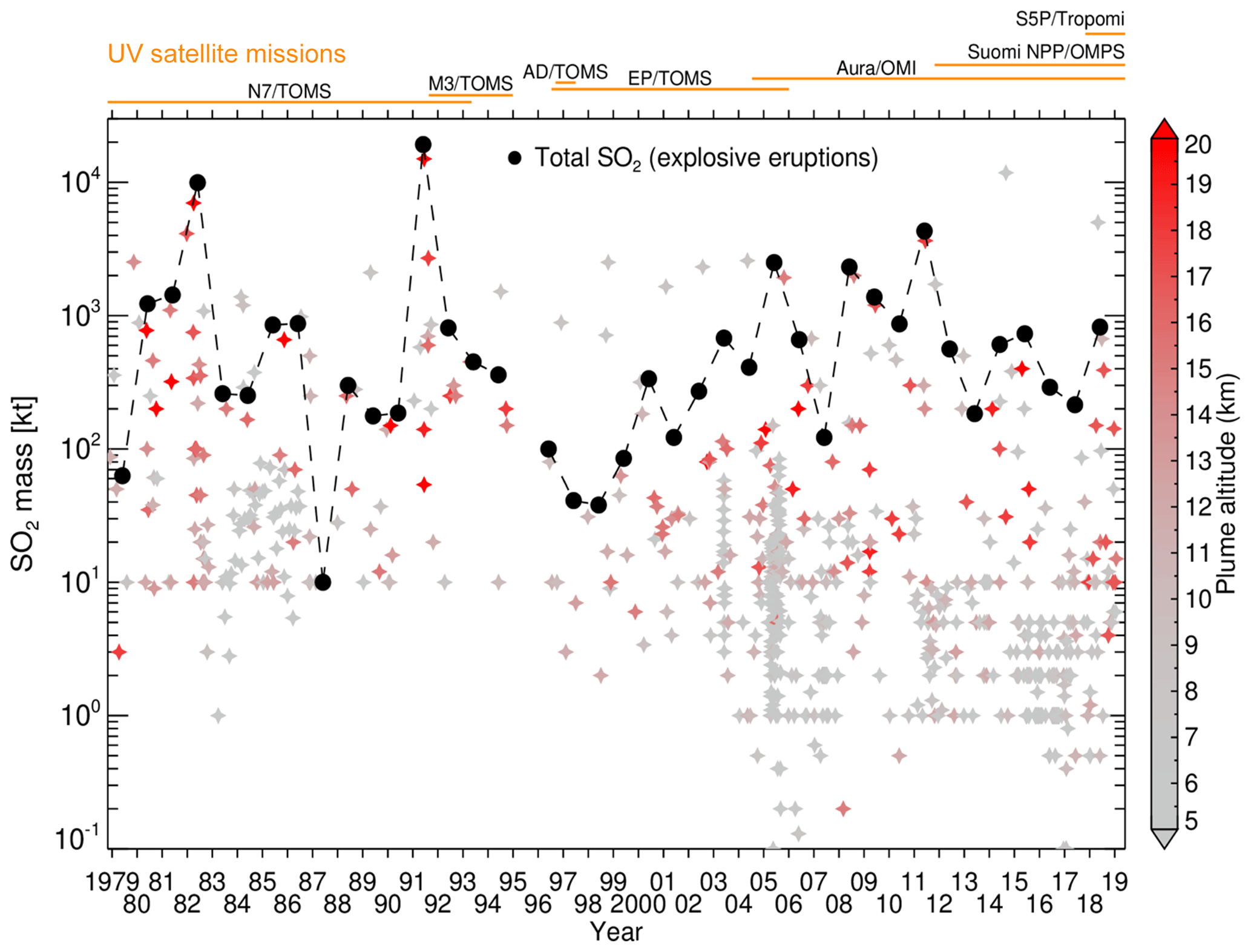
Figure 1Multi-decadal record of SO2 emissions by volcanic eruptions observed by NASA's fleet of satellites observing TOA UV radiances. Eruptions (star symbols) are color coded by estimated plume altitude and derived from a variety of sources, including Smithsonian Institution Global Volcanism Program volcanic activity reports, volcanic ash advisories and satellite data. The annual total explosive volcanic SO2 production (omitting SO2 discharge from effusive eruptions) is shown in black. The orange lines above the plot indicate the operational lifetimes of NASA UV satellite instruments: Nimbus-7 (N7), Meteor-3 (M3), ADEOS (AD), Earth Probe (EP) TOMS, OMI (currently operational), and SNPP/OMPS (currently operational), along with the ESA/EU Copernicus S5P/TROPOMI (currently operational). Data shown in this plot are available from the NASA Goddard Earth Sciences (GES) Data and Information Services Center (DISC) as a level 4 MEaSUREs (Making Earth System Data Records for Use in Research Environments) data product (Carn, 2019).
One of the key challenges in assembling a long-term, consistent, satellite-based volcanic SO2 emissions climatology (e.g., Fig. 1) is merging measurements from sensors with different spectral coverage and resolution. This complicates any analysis of “trends” in volcanic SO2 loading (e.g., in the post-2000 period of moderate volcanic eruptions; Fig. 1) or comparisons of eruptions of similar magnitude in different satellite instrumental eras. A step change in SO2 sensitivity occurred when the multispectral, six-channel TOMS instruments were superseded by hyperspectral UV sensors, such as the Global Ozone Monitoring Experiment (GOME, 1995–2003; Khokhar et al., 2005), the Scanning Imaging Absorption Spectrometer for Atmospheric Chartography (SCIAMACHY, 2002–2012; Lee et al., 2008), the Ozone Monitoring Instrument (OMI, 2004–ongoing; Krotkov et al., 2006), the Ozone Mapping and Profiler Suite (OMPS, 2012–ongoing; Carn et al., 2015), and EU/ESA Copernicus Sentinel 5 precursor (S5P) (Veefkind et al., 2012). This is manifested in Fig. 1 as an increased number of detected volcanic eruptions with low SO2 loading (< 10 kt) after 2004 (note that GOME and SCIAMACHY measurements are not shown in Fig. 1), whereas rates of global volcanic activity have not changed significantly. UV SO2 retrieval algorithms have also evolved substantially since the 1980s in response to advances from multispectral to hyperspectral sensors, improvements in ozone retrievals, and efforts to account for volcanic ash and aerosol interference (e.g., Krueger et al., 1995, 2000; Krotkov et al., 1997, 2006; Yang et al., 2007, 2010; Li et al., 2013, 2017; Theys et al., 2015). However, to date there has been no attempt to develop a single algorithm that could be used to generate a long-term, consistent SO2 climatology across multiple UV satellite missions. In this paper we describe a new multi-satellite SO2 algorithm (MS_SO2) that is applicable to both multispectral (e.g., TOMS) and hyperspectral (e.g., OMI) UV measurements. As a first step in the generation of a multi-satellite volcanic SO2 record, we apply the MS_SO2 algorithm to the Nimbus-7 TOMS (N7/TOMS) measurements (1978–1993) and present a reanalysis of some of the most significant eruptions of the N7/TOMS mission.
Ozone and SO2 are the two main absorbers in the near UV spectral region between 300 and 340 nm. The relative contributions of each gas to the satellite backscattered ultraviolet (BUV) measurements at the three absorbing TOMS channels (317, 331, 340 nm) used in the retrieval, depend on the spectral structure of the absorption cross sections, which are measured as functions of wavelength and temperature (Bogumil et al., 2003; Daumont et al., 1992). Figure 2 shows the O3 and SO2 cross sections and the SO2∕O3 cross section ratio as a function of wavelength for a spectral UV region spanning the three absorbing channels of TOMS. At the instrument's spectral resolution (∼1 nm full width at half maximum, FWHM), the SO2 molecule is 2.5 times more absorbing than O3 at 317 nm, while O3 is 6 times more absorbing at 331 nm. These differences allow for simultaneous multispectral retrievals of O3 and SO2.

Figure 2Spectral dependence of laboratory-measured SO2 (black) and O3 (red) cross sections between 310 and 340 nm at TOMS FWHM ∼1 nm. The SO2∕O3 ratio (green) is shown with the scale on the right axis. The nominal locations of the N7/TOMS absorbing bands (317, 331, 340 nm) are shown by vertical blue lines (blue).
2.1 Heritage BUV ozone algorithms
Dave and Mateer (1967) first proposed a technique to estimate total ozone column from nadir backscatter UV measurements taken in the Huggins ozone absorption band (310–340 nm), assuming no SO2 is present. Their algorithm was inspired by the pioneering Dobson spectrophotometer, which measures attenuation of solar irradiance by UV wavelength pairs from which total ozone is derived using the Beer–Lambert law. However, unlike the direct sun technique, radiative transfer calculations show that the top-of-the-atmosphere (TOA) BUV radiances (I) do not follow the Beer–Lambert law. In general, log(I) varies nonlinearly with ozone column amount (Ω), and this relationship is sensitive to the shape of the ozone profile (defined as the ozone density profile normalized to total ozone). To account for this effect, Dave and Mateer (1967) proposed constructing a set of lookup tables (LUTs) based on standard ozone profiles with different total ozone amounts using ozonesonde and Dobson Umkehr data. Since the shapes of the profiles also vary with latitude, they proposed using three sets of profiles for low latitudes, midlatitudes and high latitudes. These profiles are then used to estimate I, which varies with wavelength (λ), observational geometry, surface pressure and surface reflectivity (R). Following the Dobson convention, log(I) is converted to N value which is defined in Eq. (1) as
F is the extraterrestrial solar irradiance. By linearly interpolating N between total ozone nodes, one forms the N-Ω curves that are a single valued function of Ω representative of a given latitude band and observational geometry. This approach allows Ω to be estimated by matching the measured N value to the interpolated N values.
Over the years several modifications have been introduced to this basic concept. Mateer et al. (1971) proposed a Lambert-equivalent reflectivity (LER) concept to estimate the combined contribution of the surface, clouds and aerosols to BUV radiance. In this concept, the scene at the bottom of the atmosphere is assumed to be a Lambertian reflector, whose reflectivity (Rs) is derived from the measurements at 380 nm where the ozone and SO2 absorption is negligible. The effective pressure of this reflecting surface is assumed to vary with Rs, from a surface pressure at Rs < 0.2 to a cloud pressure 0.4 atm at Rs > 0.6, linearly interpolated at intermediate Rs. The algorithm assumed that Rs, thus derived, did not vary with wavelength. Although in the earlier versions of this algorithm wavelength pairs (313∕331, 318∕340) were used to derive Ω, Rs was later derived at 331 nm to minimize errors due to the spectral dependence of Rs. This made pairing unnecessary (McPeters et al., 1996).
By explicitly modeling the effect of aerosols using a radiative transfer code, Dave (1978) showed that Rs did not vary significantly with wavelength for non-absorbing aerosols, hence they produced no ozone error. However, for aerosols that might have strong absorption in the UV, that study predicted that Rs would decrease at shorter wavelengths, producing an overestimation of ozone. Since aerosol properties in the UV were not known at that time, no correction for aerosol absorption was applied until the mid-1990s when the effect predicted by Dave (1978) was detected in the Nimbus-7 TOMS data launched in October 1978.
Since the TOMS instrument had three reflectivity channels (331, 340, 380 nm), it was possible to compare the reflectivities derived from them. This comparison showed that Rs increased significantly with wavelength for moderately thick clouds, causing a significant underestimation of Ω (up to 3 %). A modified LER (MLER) concept assuming two Lambertian surfaces, one at the surface and the other at the cloud top was applied to minimize this error (Ahmad et al., 2004).
The most recent version of the TOMS ozone algorithm reverts back to the LER model, but it assumes that clouds are at the surface, which reduces the Rs wavelength dependence (Ahmad et al., 2004). This simple LER (SLER) model is used in our SO2 algorithm. However, since there are many other reasons for such a dependence, including ocean color, non-Lambertian surfaces, such as ocean glint and fogbow and, most importantly, the absorbing aerosol effect predicted by Dave (1978), Rs is assumed to vary linearly with λ; its slope is derived using 340 and 380 nm radiances. This simple omnibus approach works well for most cases, except when the UV absorbing aerosols (smoke, dust and volcanic ash) are very thick. Such data are flagged in the TOMS ozone algorithm. The new MS_SO2 algorithm is an extension of this algorithm into two dimensions (Sect. 3).
2.2 Heritage TOMS SO2 algorithms
Krueger (1983) was the first to suggest that TOMS could be used to retrieve sulfur dioxide from explosive volcanic events. He correctly interpreted the large positive ozone anomaly observed following the explosive eruption of El Chichón in 1982 as being due to the SO2 released into the atmosphere during the event. To estimate the SO2 inside the plume region, he separated the SO2 and O3 signals by computing a residual reflectance, estimated as the difference between the interpolated unperturbed background reflectances outside the plume and the reflectance anomaly inside the plume. This early technique for retrieving SO2 from TOMS ozone estimates became known as the residual method. The residual method, however, failed when the background could not be clearly separated from the ozone anomaly. Krueger subsequently developed the first BUV algorithm that separated the O3 and SO2 radiance contributions, based on an earlier methodology developed by Kerr et al. (1980) to retrieve the SO2 column from the ground with a Brewer spectrophotometer. This method assumed that the BUV radiation was attenuated by the two absorbing species (O3, SO2), leading to an equation describing BUV radiance, I, for a given wavelength, λ, corresponding to the TOMS field of view (FoV):
In Eq. (2), F is the incoming solar flux, Sg is the geometrical optical path (air mass factor, AMF), and and are the vertical optical thicknesses for O3 and SO2, while the coefficients a and b depend on the satellite viewing geometry, cloud or surface reflectance, and volcanic ash and sulfate aerosols (Krueger et al., 1995; Krotkov et al., 1997). Equation (2) can be expressed in matrix form, which is then inverted to obtain estimates for the SO2 and O3 vertical column densities and the dimensionless parameters a and b. This algorithm is generally referred to as the Krueger–Kerr algorithm (Krueger et al., 1995). Krotkov et al. (1997) developed radiative transfer path correction, which explicitly accounted for the Rs, ozone and SO2 vertical profiles, replacing the geometrical AMF in Eq. (2). The modified algorithm with empirical background correction has been used offline on a case-by-case basis for the past 2 decades to retrieve SO2 mass tonnage from medium to large explosive eruptions using TOMS BUV measurements (Krueger et al., 2000; Carn et al., 2003).
The new discrete wavelength SO2 algorithm (MS_SO2) builds on the heritage of the TOMS total ozone algorithm (Sect. 2.1) but adds sulfur dioxide (SO2) as a second absorber. The BUV radiance is simulated with the TOMRAD forward vector radiative transfer (RT) model (Dave, 1964) for a known viewing geometry by assuming a vertically inhomogeneous, pseudo-spherical Rayleigh scattering atmosphere with standard ozone profiles (Klenk et al., 1983; Bhartia, 2002) and a priori SO2 vertical profiles (Krueger et al., 1995). The underlying reflecting surfaces (land/ocean, clouds and aerosols) are approximated with the simple LER reflecting surface at terrain height pressure (Sect. 2.1). TOMRAD accounts for all orders of polarized Rayleigh scattering and for the gaseous absorption (e.g., O3 and SO2), using a priori vertical profiles of the gas concentrations and laboratory-measured temperature-dependent gaseous cross sections (Dave and Mateer, 1967; Bogumil et al., 2003; Daumont et al., 1992). Improvements to the TOMRAD model include corrections for molecular anisotropy (Ahmad and Bhartia, 1995), rotational Raman scattering (Joiner et al., 1995) and pseudo-spherical corrections to account for changes to the solar and viewing zenith angles due to the sphericity of the Earth.
Table 1Input parameters used in construction of the Nimbus-7 TOMS LUTs.
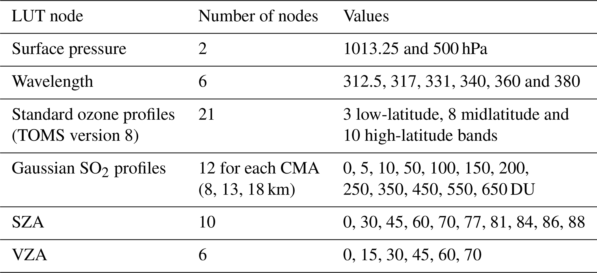
Performing online radiative transfer calculations for every satellite field-of-view (FoV) can greatly increase the time required to process full orbits of data. To improve the computational efficiency of the operational algorithm, N7TOMS-specific lookup tables (N7TOMS-LUT) were produced offline using the inputs listed in Table 1 and convolved with the triangular band pass at each of the six Nimbus-7 TOMS wavelengths (FWHM ∼1 nm).
The TOMRAD algorithm was configured to account for two absorbing trace gases: O3 and SO2. The LUTs include 21 total ozone nodes and 12 total SO2 nodes for each of the three assumed SO2 heights. For ozone, the total column amounts and profile shapes vary between latitude bands (see Table 1). For sulfur dioxide, we assumed a Gaussian vertical profile shape, which is determined by two parameters: a center of mass altitude (CMA) and a geometrical standard deviation. The CMA represents the altitude of the peak SO2 concentration. LUTs for SO2 are generated for three different CMAs: 8 km (middle troposphere, TRM), 13 km (upper tropospheric, TRU) and 18 km (lower stratospheric, STL). A constant standard deviation of σ=2 km is assumed for each SO2 profile.
The MS_SO2 algorithm retrieves a four-parameter state vector, x,defined below as
where Σ is the retrieved total column sulfur dioxide, Ω is the total column ozone, dR∕dλ characterizes the Rs spectral dependence between 340 and 380 nm, and Rs is the LER at 380 nm. The retrieval of sulfur dioxide is carried out in one or two steps described in the next sections, referred to as step 1 and step 2.
3.1 Step 1 retrieval
Our step 1 inversion starts with an initial state vector x0, consisting of first guesses for Σ0, Ω0 and dRs0∕dλ shown in Table 2. The final state vector, x, is determined iteratively by inverting the Jacobian matrix K at each iteration step:
where dx represents the relative changes in the state vector from the previous iteration and dN represents the residual vector equal to Nm−Nc, computed as the difference between the measured N values, Nm, and the calculated N values, Nc, at the four TOMS channels at 317, 331, 340 and 380 nm. K represents a 4×4 Jacobian matrix computed from the LUTs. These matrix elements are defined as follows:
where Nc,i is the forward model calculated N value at wavelength i.
The reflectivity Rs is computed analytically using the measured BUV radiance at 380 nm (see Supplement, Eq. S4). Note that since the O3 and SO2 cross sections are negligible at 380 nm, the Rs and do not change with the iterations (i.e., dRs=0).
Equation (4) is solved iteratively by zeroing the residuals, dN=Nm-Nc, and recomputing the Nc and the Jacobians at each iteration step for the four used channels. The state vector is then adjusted after each iteration, , ,… until it converges on a solution as described below:
Since O3 and SO2 exhibit small absorption at 340 nm, a nonzero R spectral slope (i.e., ) accounts for the radiative effects of aerosols and surface reflectance (e.g., sun glint).
Table 2Retrieved state vector. n/a – not applicable.
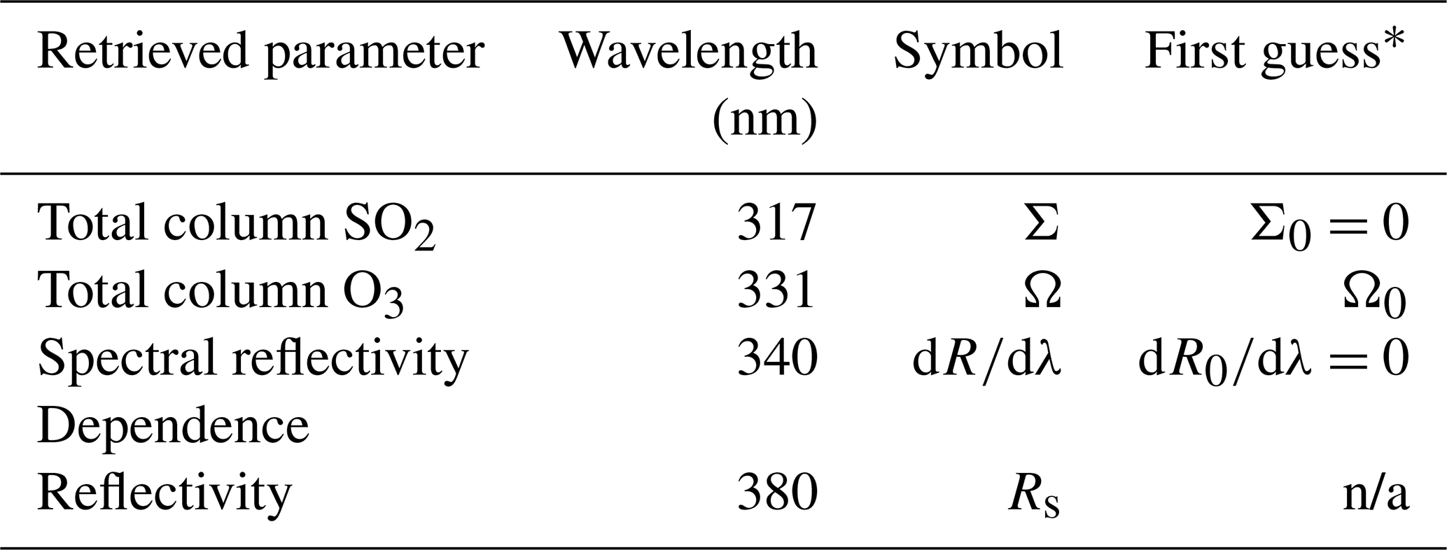
*Ω0 is a climatological value for each of the three latitude bands.
As indicated in Table 2, the algorithm initially assumes zero R-λ dependence (i.e., ); however, absorbing aerosols (smoke, dust and volcanic ash) cause .
The algorithm uses retrieved spectral slope dR∕dλ in Eq. (7) below to update the calculated LERs after each iteration:
where λj=312, 317, 331, 340 nm and λR=380 nm. When SO2 or aerosol loading is high nonlinear R-λ dependence can cause systematic errors in the retrieval state vector. For this reason, we do not use the shortest 312 nm channel in the retrievals (Eqs. 5–6), but the final residual dN312 is used as a diagnostic of the nonlinearity. A step 2 empirical procedure, described in the next section, was developed to correct for the retrieval bias resulting from these errors.
3.2 Step 2 retrieval
The MS_SO2 forward model accounts for O3 and SO2 absorption and linear spectral changes in Rs due to the presences of aerosols. The algorithm, however, does not explicitly characterize the absorption and scattering effects of volcanic ash (absorbing) and sulfate (non-absorbing) aerosols. The retrieval errors in Σ and Ω caused by volcanic ash during the first few days after an explosive eruption can be significant in the case of major volcanic eruptions like Pinatubo and El Chichón (Krueger et al., 1995; Krotkov et al., 1997). A step 2 procedure was developed primarily to handle explosive eruptions (Volcanic Explosivity Index, VEI > 3 ), in which large Ω anomalies are identified to occur in conjunction with high ash concentrations. In step 2, a corrected total ozone Ωcor inside the SO2 cloud is interpolated using the retrieved Ω outside the plume along the orbit for each cross-track position. Even if ozone-destroying chemicals are present, such effects can still be considered negligible over the relatively short time periods that SO2 concentrations are high enough to affect TOMS observations.
In deciding whether to apply step 2, the algorithm considers the retrieved Σ, Ω and aerosol index (AI) in Step 1. The AI is estimated from the dR∕dλ and the calculated Jacobian dN∕dR at 340 nm:
Positive AI (dR∕dλ > 0) identifies spatial regions affected by absorbing aerosols (dust, smoke and ash). The step 2 selection criteria first select FoVs where either SO2 > 15 DU (inside the plume) or AI > 6. The additional AI criterion allows for the selection of FoVs around the edges of the cloud, where the SO2 can be less than 15 DU due to high aerosol concentrations. In this case, it is assumed that the step 1 SO2 may have been underestimated due to the ozone error caused by high aerosol concentrations (in these cases, the SO2 retrieved in step 2 may still not exceed 15 DU and therefore would be excluded from the plume in subsequent mass calculations). We describe the methodology for interpolating Ωcor in Eqs. (S5)–(S7). A second retrieval of SO2 and dR∕dλ is then performed by inversion using the measured 317 and 340 nm radiances while treating the ozone Ωcor as a constant. This constraint on the ozone bounds the SO2 Jacobians computed from the forward model LUTs. The operational MS_SO2 product files include a step 2 algorithm flag (not applied =0, applied =1).
To illustrate the effects of the step 2 procedure, we consider the 1982 explosive eruption of El Chichón, which emitted ∼7 Tg SO2 (Krueger et al., 2008) the second largest observed in the satellite era (Fig. 1). Figure 3 shows the retrieved AI map during TOMS overpass of the volcano on 4 April 1982, while it was still erupting. High AI values exceeding a value of 10 correspond to biased high step 1 ozone values (Fig. 4a) and underestimated Σ values (Fig. 4c). Figure 4b shows the step 2 corrected Ωcor, making it consistent with the Ω field outside of the volcanic cloud. Figure 4d shows the step 2 Σ, which is much higher than step 1. As can be seen in this particular example, the step 2 correction can significantly increase the SO2 mass. In this case, the SO2 mass increased from 2475 (step 1) to 3637 kt (step 2). Peak Σ values increased from 396 to 549 DU in the aerosol affected region. The biases, dΩ and dΣ, for this case are shown in Fig. S1 in the Supplement. Step 2 was developed primarily to handle extreme eruptions (VEI > 3), such as El Chichón and Pinatubo, where large Ω anomalies sometimes occur in conjunction with high ash concentrations. In practice, step 2 corrections tend to be small (or nonexistent) for most of the eruptions detected observed during the observation period covered by TOMS.
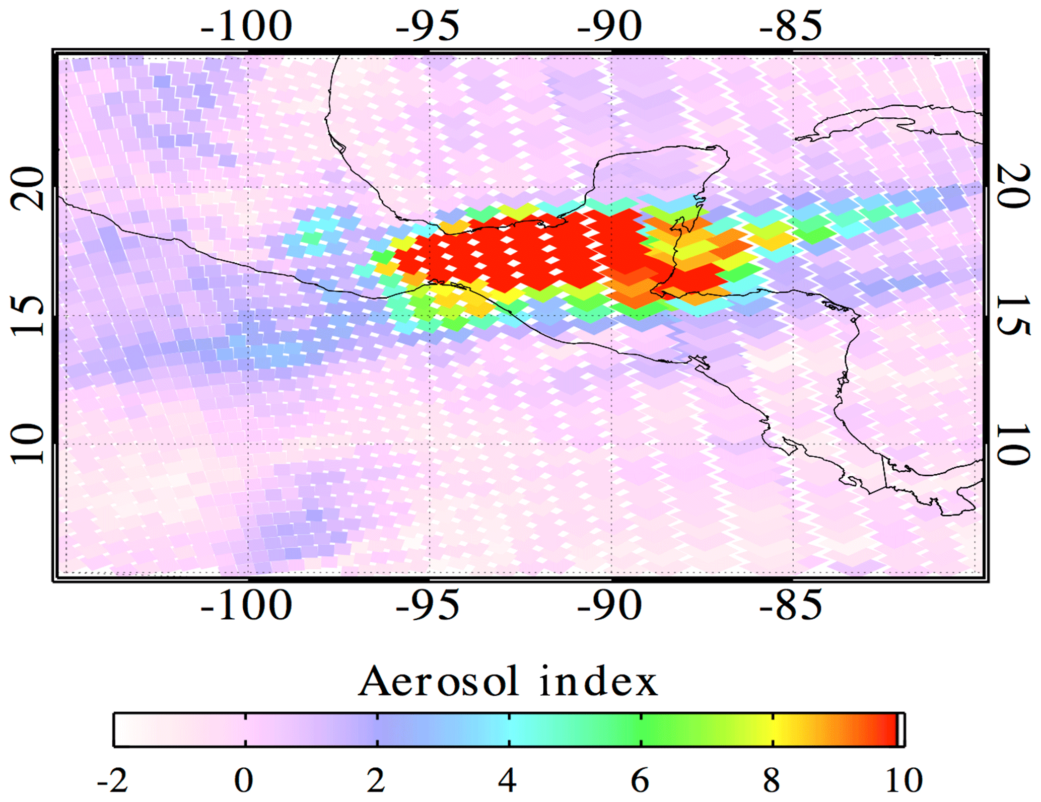
Figure 3Aerosol index for the El Chichón eruption on 4 April 1982, computed from retrieved dR∕dλ.
The corrected step 2 Ω values inside the volcanic cloud shown in Fig. 4b appear to be fairly consistent with the regional unperturbed ozone field, but it should be noted that a few remaining high Ω values in the boundary of the plume still exist, which were not selected for step 2 (Fig. 4b). These pixels were not corrected because the threshold criteria were not met, thus Σ may be underestimated. However, their contribution to the total SO2 cloud mass is insignificant.
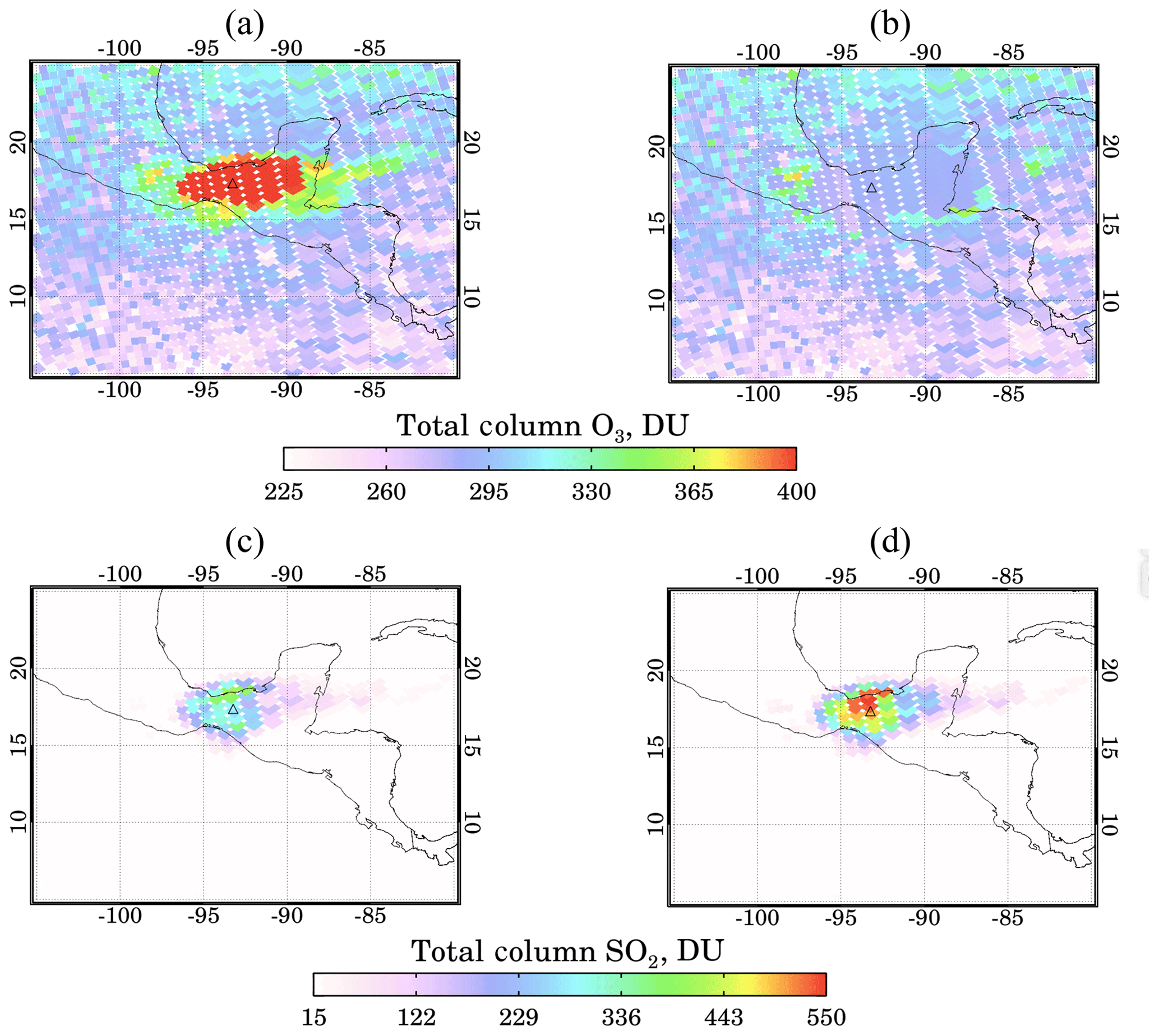
Figure 4MS_SO2 maps showing (a) step 1 total column O3, (b) step 2 total column O3, (c) step 1 total column SO2 and (d) step 2 total column SO2 from the El Chichón eruption on 4 April 1982.
Step 2 follows a methodology similar to the original residual method developed by Krueger (1983), which separated the O3 and SO2 contributions by subtracting the measured BUV reflectance in the unperturbed region from the BUV radiance anomaly associated with the SO2 cloud. The MS_SO2 algorithm corrects the overestimated step 1 ozone inside the plume by correcting the positive ozone bias. Our step 2 procedure is typically only applied when the ash and/or SO2 loading causes the reflectivity dependence to become nonlinear, as the forward model does not explicitly account for volcanic aerosol absorption. This scenario typically lasts for about 1–3 d following a major explosive eruption, during which total retrieved SO2 mass is likely to be underestimated and in some cases could even increase with time due to ash and ice fallout and plume dispersion. For such extreme cases we recommend estimating SO2 to sulfate conversion e-folding lifetime using weeks of measurements of the total SO2 cloud daily mass and extrapolating it back in time to estimate total SO2 mass emitted on eruption day. This “day one” time extrapolated SO2 mass is typically larger than retrieved on days immediately following the eruption (Krotkov et al., 2010).
3.3 Soft calibration: N value bias correction
We assume that the background sulfur dioxide is below TOMS detection limit in regions of the atmosphere far away from SO2 sources (e.g., volcanic, anthropogenic). Random errors associated with the retrieval process, however, are normally distributed around zero. We expect that the true volcanic SO2, Σtrue and the mean of the distribution, 〈Σ〉clean, to equal zero such that
We examined a sample of 90 TOMS orbits in clean regions of the central Pacific Ocean and found a positive bias of about 3 DU (i.e., 〈Σ〉clean∼3 DU, Fig. 5). A soft calibration procedure was developed for correcting this bias by applying a small constant N340 value adjustment to the measured 340 nm BUV radiances. The details of this procedure are described in Sect. S3.3 in the Supplement. Figure 5 shows probability density functions (PDFs) of the step 1 SO2 before (dashed) and after (solid) applying the correction for 11 November 1981. The mean bias is reduced to < 1 DU after applying the correction.
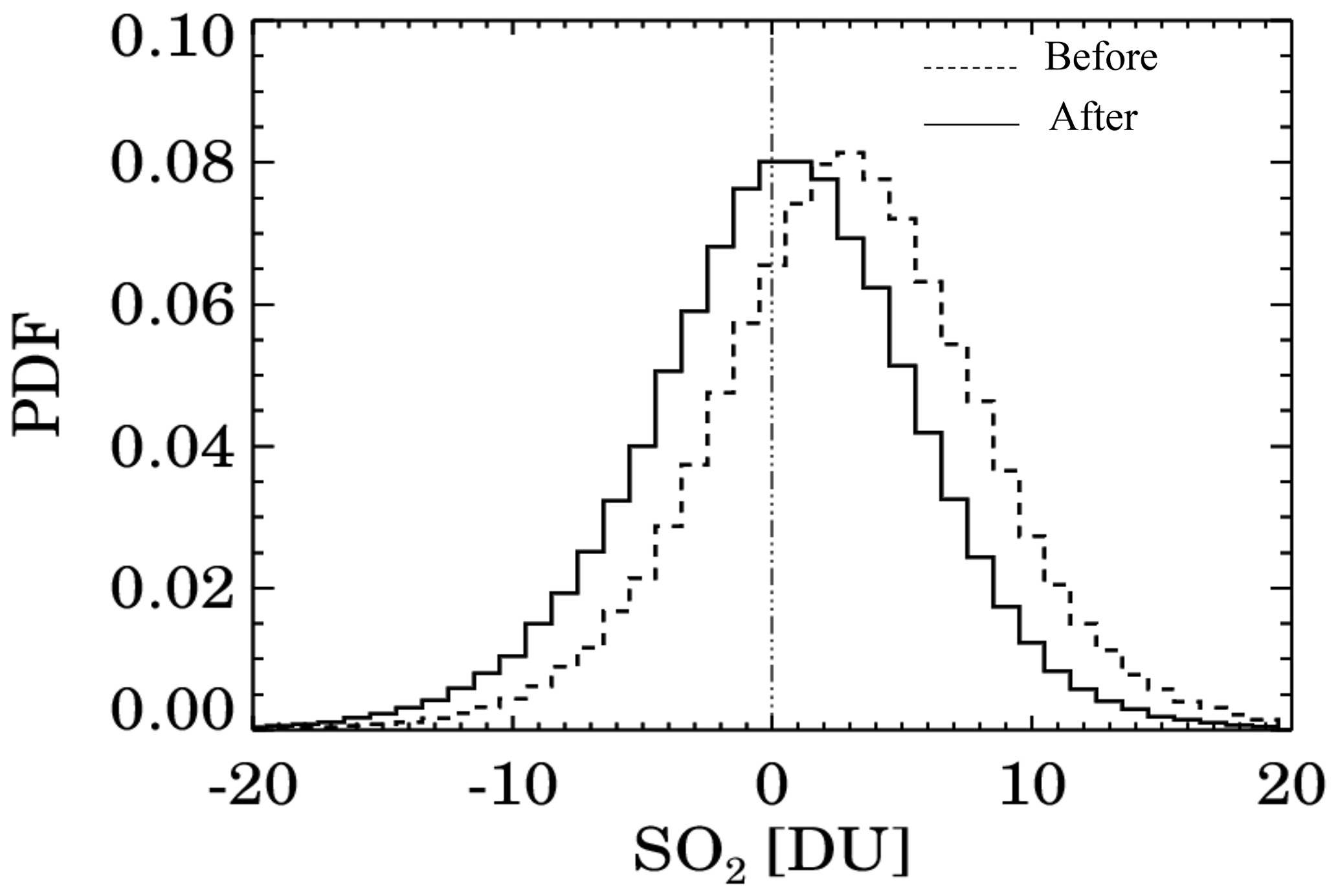
Figure 5Probability density function of SO2 background before (dashed) and after (solid) applying N340 value correction.
4.1 Random errors and SO2 detection limit
The random errors in the MS_SO2 retrieval were estimated from the standard deviation in the SO2 from a large data sample that included 90 central Pacific orbits, spanning a 10-year period between 1980 and 1990. Data were restricted to Σ values between −20 and 20 DU (Fig. 6a). Standard deviations were then computed as a function of the TOMS swath position, as shown in Fig. 6b. Figure 6b can be used to characterize the SO2 detection limits for TOMS. In this section, we compare the TOMS error distribution with the UV Ozone Mapping Profile Suite Nadir Mapper (OMPS-NM), a hyperspectral UV instrument onboard the Suomi National Polar-orbiting Partnership (NPP) and NOAA 20 satellites. For this comparison, we selected 1 month of NPP/OMPS spectral data (central Pacific) and applied the MS_SO2 algorithm using the same four wavelength bands of TOMS (Table 2), which were first convolved with the TOMS bandpass function.
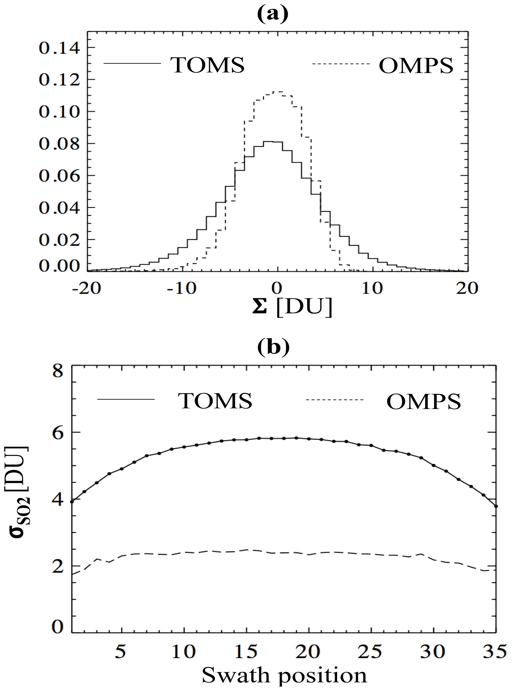
Figure 6(a) PDF of SO2 background (noise distribution) for TOMS and OMPS based on orbits from clean regions of the central Pacific, and (b) standard deviations of background SO2 for TOMS and the OMPS nadir mapper as a function of the swath position. OMPS noise is more than a factor of 2–3 lower than TOMS and less dependent on cross-track position.
Figure 6b shows that TOMS retrieval noise depends on the swath position, varying from ∼6 DU at nadir to ∼4 DU at higher viewing angles, while OMPS is 2–3 times smaller (∼2 DU) and is relatively independent of the cross-track position. Using the MS_SO2 algorithm, we subsequently estimate the SO2 detection limit for TOMS and OMPS-NM to be about 15 DU and 6 DU (∼99 % confidence level), respectively. We note that when applying the Principal Component Algorithm (PCA) (Li et al., 2013) to all the 100–200 wavelengths available from OMPS-NM hyperspectral measurements, the noise is reduced by an order of magnitude to ∼0.2–0.5 DU, allowing detection of large anthropogenic point sources (emissions more than ∼80 kt yr−1) (Zhang et al., 2017).
4.2 Systematic errors in volcanic SO2 plumes
In this section, we evaluate systematic errors of the MS_SO2 retrievals of volcanic SO2. The two most significant errors are caused by volcanic aerosols (ash and sulfate) and incorrect assumptions regarding the SO2 profile, namely the plume height. The radiance tables used by the algorithm account for ozone and SO2 absorption but do not account for the absorption and scattering by aerosols. The ash errors can be significant during the first couple days after the initial eruption phase (Rose et al., 2003; Guo et al., 2004). The precomputed radiance tables used by MS_SO2 assume an SO2 column amount and an a priori CMA and standard deviation (Sect. 3). An incorrect CMA assumption can cause significant SO2 errors that vary with viewing geometry, ozone and SO2 column amounts. We characterize these error sources by applying the MS_SO2 algorithm to synthetic radiances.
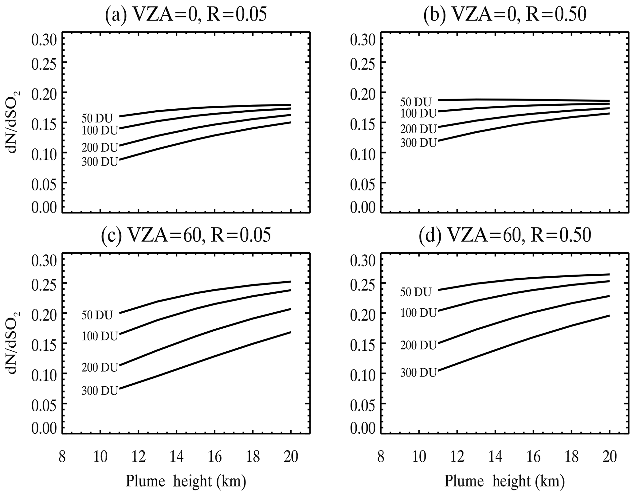
Figure 7VLIDORT calculated SO2 column Jacobians () at 317 nm for typical conditions in the tropics (SZA , relative azimuthal angle, RAA , O3=275 DU) but different SO2 column amounts (50, 100, 200 and 300 DU) and center mass altitudes (11–20 km). For these calculations, Gaussian SO2 profiles with the same standard deviation (2 km) were assumed: (a) VZA =0 and R=0.05, (b) VZA =0 and R=0.50, (c) VZA =60 and R=0.05, and (d) VZA =60 and R=0.50.
4.2.1 Uncertainties due to SO2 plume height
To understand retrieval errors in MS_SO2 algorithm due to assumed a priori SO2 profiles, we conducted sensitivity tests using the VLIDORT radiative transfer code for the typical observational conditions in the tropics, midlatitudes and high latitudes. Figure 7 shows column SO2 Jacobians at 317 nm for different SO2 amounts, Σ, nadir angles and scene reflectance as function of the assumed SO2 height (center of mass altitude, CMA). The Jacobians generally increase with the CMA, meaning that satellite BUV measurements are more sensitive to SO2 at higher altitudes. This means that the MS_SO2 algorithm will overestimate (underestimate) the SO2 column amount if the CMA of the a priori profile is lower (higher) than that of the actual SO2 profile. On the other hand, the sensitivity of SO2 Jacobians with respect to CMA is affected by several other factors, particularly SO2 column amounts, geometry (solar zenith angle and viewing zenith angle), the reflectivity of the underlying surface (Rs) and the CMA itself. In general, the sensitivity of SO2 Jacobians to CMA is greater for SO2 plumes with large SO2 loading (e.g., 300 DU vs. 50 DU) at relatively low altitudes (e.g., CMA of 13 km vs. 18 km), lower reflectivities (e.g., Rs of 0.05 vs. 0.50) or at high viewing angles relative to the nadir (e.g., VZA of 60∘ vs. 0∘). For calculations assuming typical midlatitude and high-latitude conditions, we found similar sensitivities of SO2 Jacobians to CMA. From these calculations, we can estimate the errors in the SO2 Jacobians at 317 nm, assuming that the standard a priori profiles used in MS_SO2 retrievals (CMA: 13 and 18 km) have a ±2 km error in CMA. The results for the tropics, midlatitudes and high latitudes are summarized in Tables S1, S2 and S3, respectively, in the Supplement. As shown in the tables, for SO2 plumes from relatively moderate eruptions (∼50 DU), the relative errors in SO2 Jacobians due to the error in the CMA are mostly within ±10 %. But for plumes with large SO2 loading (∼200–300 DU) from explosive eruptions such as Pinatubo, the relative error in SO2 Jacobians may reach as high as 30 % for pixels near the edge of the swaths that have low reflectivity. Additionally, for pixels with the same reflectivity and VZA, the relative errors due to SO2 height are greater for midlatitude and high-latitude eruptions than for tropical eruptions.
To quantify the retrieval errors due to inaccuracies in the a priori profiles, we used the top-of-the-atmosphere synthetic radiance data generated by VLIDORT as input to the MS_SO2 algorithm. The retrieved SO2 and O3 column amounts were compared with assumed in VLIDORT calculations (Tables S4–S7). As shown in the tables, for SO2 plumes with a modest loading (∼50 DU), the relative errors in SO2 column amounts, due to a 2 km error in the a priori profile are typically 10 % or less, whereas the relative errors in O3 are within 1 %. For plumes with large SO2 loadings (200–300 DU), the errors in SO2 amounts due to a 2 km bias in the a priori profile are typically 5 %–15 % but can reach as high as 30 %–40 % for high-latitude plumes with large SZA and VZA. For extreme conditions at high latitudes (Table S5, 13 km a priori profile vs. 15 km actual profile, SO2=300 DU), the MS_SO2 algorithm failed to converge after 20 iterations, due to a signal saturation caused by strong absorption at 317 nm. In these relatively rare cases, it is beneficial to use longer wavelengths (e.g., > 320 nm) for SO2 retrievals (Li et al., 2017; Theys et al., 2015), which are available from the current hyperspectral instruments such as OMI and OMPS but not TOMS.
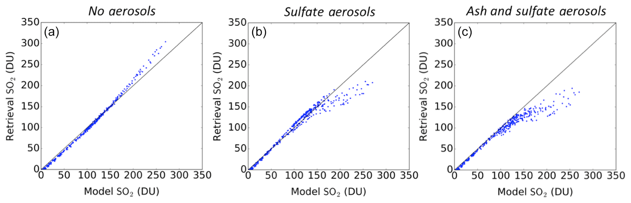
Figure 8Comparison of the OMPS retrieval SO2 against the GEOS-5 model SO2. The TOA radiances for the OMPS retrieval were generated assuming no aerosol (a), only sulfate aerosols (b), and both ash and sulfate aerosols (c).
We also calculated the residual at 312 nm (res), defined here as the difference between the “measured” synthetic Nm and the Nc at 312 nm using MS_SO2 retrieved ozone and SO2 column amounts. Note that the 312 nm channel was not used in the MS_SO2 algorithm, and the residuals at other wavelengths are essentially zero since we are retrieving four parameters from four wavelengths. As shown in Tables S4–S7, a positive bias in the SO2 height (when the is CMA too high when compared with the actual profile) leads to negative residuals at 312 nm, whereas a negative bias in a priori profile (CMA too low) causes positive residuals. The residuals are generally within 1–2 N value (2 %–5 % error in radiance) for SO2 column amounts of 50–100 DU but can reach 3–7 N value (6 %–15 %) for large SO2 amounts of 200–300 DU. While the 312 nm channel may potentially be used to retrieve SO2 plume height for large volcanic eruptions, it is strongly affected by volcanic aerosols as demonstrated in the next section.
4.2.2 Ash and sulfate aerosol effects on MS_SO2 retrievals
To test the sensitivity of the MS_SO2 algorithm to ash and sulfate aerosols, an Observing System Simulation Experiment (OSSE) was conducted. The experiment used the GEOS-5 Earth system model (Molod et al., 2012; Buchard et al., 2017; Colarco et al., 2012), coupled with online Goddard Chemistry Aerosol and Radiation (GOCART) (Chin et al., 2000; Colarco et al., 2010) and Community Aerosol and Radiation Model for Atmospheres (CARMA) (Toon et al., 1988; Colarco et al., 2014). In this experiment, we considered three separate cases for a Pinatubo-like eruption scenario: (1) 12 Mt of SO2 and no aerosols; (2) 12 Mt of SO2 and 4 Mt of sulfate aerosols (as reported by Guo et al., 2004); and (3) 12 Mt of SO2, 4 Mt of sulfate aerosols, and 5 Mt of ash uniformly distributed between 18 and 22 km above the location of Pinatubo volcano, on 15 June 1991, from 06:00 to 15:00 UTC.
The GEOS-5 simulated 4-D profiles of ozone, SO2, sulfate aerosols and volcanic ash were used as input to a VLIDORT RT model (Spurr, 2008). The model generated synthetic radiances at 317, 331, 340 and 380 nm TOMS bands, using the actual Suomi National Polar Partnership (SNPP)/OMPS-NM viewing geometry, assuming cloud-free conditions. The synthetic radiances produced by the VLIDORT were used as input to the MS_SO2 algorithm to generate “retrieved” columns of ozone and SO2. We note that MS_SO2 algorithm uses LUTs produced using a different TOMRAD RT model.
Figure 8 compares retrieved versus true SO2 column amounts for the three cases considered. The retrieval bias is inferred from the differences between the model SO2 input and the SO2 retrieved by MS_SO2, using the radiances from the model run. The no aerosol case confirms unbiased SO2 retrievals for SO2 column amounts less than ∼150 DU and small positive bias for larger SO2 amounts. For aerosol cases where sulfates and ash were included in the simulation, we observe a negative bias for SO2 column amounts exceeding ∼100 DU. These negative biases (retrieval saturation) are expected as the MS_SO2 forward model does not explicitly account for volcanic aerosols. This OSSE experiment shows the effects of heavy aerosol loading on the retrieval but also increases confidence in MS_SO2 retrievals between 15 and 100 DU, under nominal conditions, even in the presence of high aerosol concentrations.
We directly compared MS_SO2 retrievals with the principal component analysis (PCA) SO2 algorithm adapted to the TOMS 6 spectral channels. In the PCA approach (Li et al., 2013, 2017), a set of principal components (PCs) is first extracted from the measured radiances using a PCA technique and ranked in descending order according to the spectral variance they each explain. If derived from SO2-free areas, these PCs represent geophysical processes (e.g., ozone absorption) and measurement details (e.g., wavelength shift) that are unrelated to SO2 but may interfere with SO2 retrievals. Next, we fit the first nν (non-SO2) PCs and the SO2 Jacobians () to the measured radiances (in N value) described in Eq. (10). This allows us to simultaneously estimate the coefficients of the PCs (ω) and SO2 column amount and helps to minimize the impacts of various interfering processes:
A more detailed introduction to the PCA SO2 retrieval technique for hyperspectral instruments such as the Ozone Monitoring Instrument (OMI) and the Ozone Mapping and Profiler Suite Nadir Mapper (OMPS-NM) can be found elsewhere (e.g., Li et al., 2013, 2017; Zhang et al., 2017).
For this comparison we adapt the PCA to the discrete wavelength of N7/TOMS. The Nimbus-7 TOMS PCA SO2 algorithm is similar to the OMI and OMPS-NM version in terms of its overall structure but differs in some implementation details. Specifically, unlike the OMI/OMPS volcanic SO2 retrievals that use a dynamic spectral fitting window (Li et al., 2017), the TOMS PCA SO2 algorithm uses all six wavelengths available from TOMS in fitting. Also due to the small number of wavelengths, in the TOMS PCA SO2 algorithm, we always use nν=5 PCs in Eq. (10), lower than the number of PCs used for OMI (nν≤20) or OMPS (nν≤15). For OMI and OMPS retrievals, SLER is derived at three wavelengths (342, 354 and 367 nm) and extrapolated to other wavelengths using a second-degree polynomial function fitted to these three wavelengths. As for TOMS, SLER is determined at 340 and 380 nm and extrapolated linearly. Additionally, while the Jacobian lookup tables are constructed using the VLIDORT radiative transfer code (Spurr, 2008) for both OMI/OMPS and Nimbus-7 TOMS, different, instrument-specific slit functions are used to band-pass the SO2 Jacobians from the lookup tables.
We compared retrievals from the two algorithms for the first 6 d of Mount Pinatubo eruption (16–21 June 1991). The Pinatubo case provides a large sample of FoVs spanning a broad range of SO2 amounts from 15 DU (minimum threshold) to over 400 DU. In this test of the algorithm, MS_SO2 and PCA retrievals were generated assuming a CMA of 18 km.
June 1991 eruption of Mount Pinatubo
Mount Pinatubo is a large stratovolcano located at 15∘08′ N, 120∘21′ E in western Luzon, Philippines, that erupted explosively on 15 June 1991, following weeks of precursory activity. TOMS SO2 imagery on 15 June shows a narrow, elongated SO2 ash plume extending to the west from the location of the volcano. On the following day TOMS measured a massive SO2 plume to the west of the volcano (Bluth et al., 1992). TOMS continued tracking the daily evolution of the Pinatubo volcanic cloud as it encircled the Earth over a period of about 22 d. Previous estimates of the Pinatubo SO2 height (CMA) range between 18 and 25 km (Self et al., 1996; Guo et al., 2004).
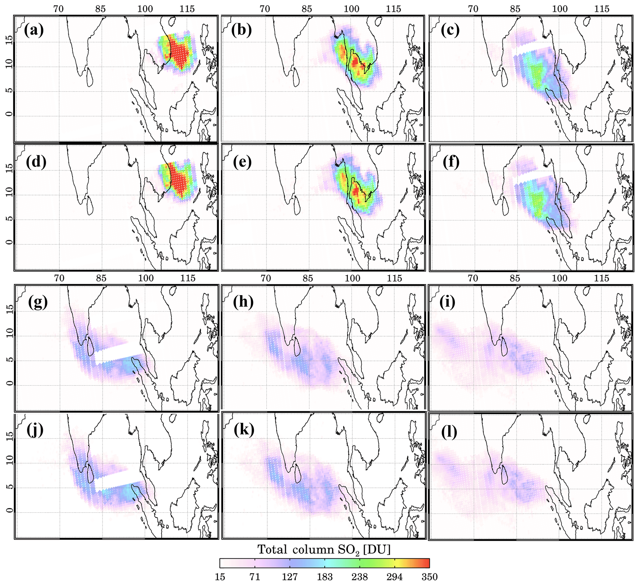
Figure 9Daily SO2 imagery for MS_SO2 and the PCA using data from TOMS overpasses of the Pinatubo eruption cloud between 15 and 21 June 1991: (a) MS_SO2 for 16 June and (b) MS_SO2 for 17 June, (c) MS_SO2 for 18 June and (d) PCA for 16 June, (e) PCA for 17 June and (f) PCA for 18 June, (g) MS_SO2 for 19 June and (h) MS_SO2 for 20 June, (i) MS_SO2 for 21 June and (j) PCA for 19 June, and (k) PCA for 20 June and (l) PCA for 21 June.
Figure 9 shows TOMS daily SO2 maps produced with the MS_SO2 and the PCA algorithms for the 6 d period from 16 to 21 June. Corresponding ash index (AI) imagery from MS_SO2 is shown in Fig. 10. SO2 and AI imagery for 16 June show a large SO2 ash cloud propagating to the west. AI values range from 4 to above 12 across the plume. The AI values decreased over the following days due to wind advection and wet deposition (Guo et al., 2004). As the SO2 cloud area continues to expand, total SO2 mass remains high, while SO2 peak values decrease, which is expected from cloud dispersion. The MS_SO2 and the PCA imagery show excellent qualitative agreement in resolving the plume area and internal SO2 plume structure, as inferred from the SO2 gradients across the peak regions of the cloud. Note that for 16–19 June, part of the observed cloud is missing due to a known mechanical problem with the TOMS instrument. These missing regions can be clearly identified in the imagery.
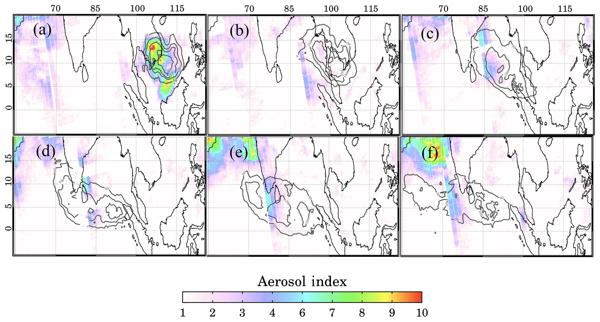
Figure 10Daily AI imagery retrieved using MS_SO2 between 16 and 21 June 1991. Contours show SO2 levels from Fig. 9. Positive AI values over India and the Arabian peninsula are due to dust aerosols, not related to the Pinatubo ash cloud: (a) 16 June, (b) 17 June, (c) 18 June, (d) 19 June, (e) 20 June and (f) 21 June.

Figure 11Scatterplot of retrieved SO2 using PCA and MS_SO2 algorithms for the period 16–21 June 1991.
Figure 11 shows a scatterplot comparing the MS_SO2 and PCA retrievals for the 6 d time series, which included over 7000 matching FoVs. These results show the retrievals are in close quantitative agreement, with a correlation of 0.993 and a slope of 1.00. Since the two algorithms apply fundamentally different approaches to retrieving SO2, this level of agreement is impressive considered over such a broad range of values.
Table 3Daily SO2 mass and maximal SO2 values for MS_SO2, PCA and KK algorithms for the 6 d following the Pinatubo eruption on 15 June 1991.
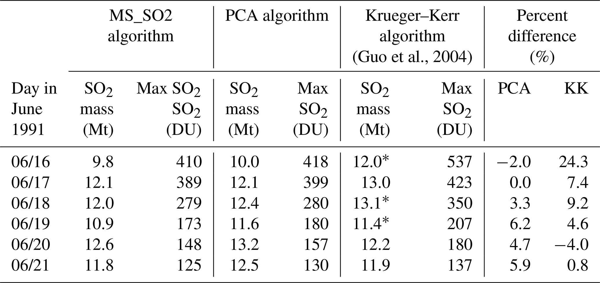
* Guo et al. (2004) interpolated values in the missing data region seen in maps for 16, 18 and 19 June.
We further compared quantitative estimates of SO2 cloud mass, peak SO2 and plume area. For this comparison, we also considered results from the Krueger–Kerr algorithm (KK), based on the published results of Guo et al. (2004). Table 3 displays daily estimates of the SO2 cloud mass and peak SO2 amounts for the MS_SO2, PCA and KK algorithms for the 6 d period. Guo et al. (2004) applied a modified version of the KK algorithm that assumes a radiative transfer air mass factor (AMF), which accounts for the a priori ozone and SO2 absorption profiles (Krotkov et al., 1997). The early SO2 mass estimates by Bluth et al. (1992) derived from Pinatubo eruption assumed a geometrical AMF. Also note that Guo et al. (2004) interpolated across the missing data regions of the plume on 16, 18 and 19 June using a punctual kriging statistical analysis. Here, we did not correct for the missing data. The three algorithms are in good overall agreement for the period from 17 to 21 June, with the differences within 10 % compared to MS_SO2. The most significant differences between the three algorithms are observed on 16 June under conditions of heavy ash loading. KK mass tonnage estimates exceeded MS_SO2 by over 24 % even though MS_SO2 and the PCA differ by just 2 %. Some of the difference between KK and the other two algorithms can be attributed to the fact that the Guo et al. (2004) estimates include contribution from the missing data region at the northern boundary of the plume (compare SO2 and aerosol imagery), but this contribution does not nearly account for the total difference in Table 3.
The differences can be explained by considering how each algorithm is affected by aerosols. MS_SO2 accounts for ash by retrieving the spectral dependence at 340 nm, which is then adjusted iteratively to correct the reflectivity at the two absorbing channels. As explained in Sect. 3.2, absorbing aerosols in the column can cause possible ozone anomalies, which decrease Σ. The KK algorithm (Krueger et al., 1995) accounts for ash implicitly by retrieving two linear spectral parameters that adjust calculated Nc to match measured Nm. Like MS_SO2, the KK radiative path LUTs are based on TOMRAD calculations that do not explicitly account for ash (Krotkov et al., 1997). Krueger et al. (1995) estimated that ash aerosols can cause errors in the retrieval up to +30%, depending on the ash size distribution. The PCA algorithm, in contrast, accounts for ash in the separation and ordering of the principal components. The differences between MS_SO2 and KK on 16 and 17 June can be partly ascribed to the effects of aerosols on the retrievals.
By 18 June, the ash and SO2 clouds have mostly separated, though, aerosol indices over 4 are still observed in some regions of the plume. Pinatubo did not erupt again after the major eruption on 15 June, yet the three algorithms show retrieved SO2 mass increases on 17 and 20 June (the PCA and KK retrievals also indicate a small increase on 18 June). Guo et al. (2004) attribute these increases to the sequestering of volcanic SO2 by ice–ash mixtures in the plume. They propose the sequestered SO2 was released at a later time through sublimation of ice in the lower stratosphere. The oxidation of hydrogen sulfide offers another mechanism to account for the observed mass increases in the days following the eruption. The combined results of the three algorithms support the conclusions of Guo et al. (2004) that the observed mass increases in the temporal evolution of the plume are real.
Overall, the PCA retrieved 3 % more total mass tonnage than MS_SO2. These differences are attributed to differences in how the MS_SO2 algorithm handles aerosols and differences in the area of the plume due to differences in the retrieval near the sensitivity threshold (∼15 DU). Ash, sulfates and high SO2 amounts impact the ozone retrieval, for as was seen in Sect. 3.2, systematic errors in SO2 are anticorrelated with errors in O3 (see Fig. S1). For the case of the KK algorithm, the total ozone retrieved inside the SO2 plume can be unrealistically low and even negative in an extreme event like Mount Pinatubo shown in Figs. S4 and S5. Figure S4 compares the KK ozone retrieval with MS_SO2 step 2 ozone retrieval and Fig. S5 compares scatterplots of SO2 and total ozone for 17 and 18 June.
Table 4SO2 plume area and number of fields of view (NFoVs) where the retrieved SO2 exceeded 15 DU using the MS_SO2 and PCA algorithms for the 6 d following for the Pinatubo eruption on 15 June 1991.
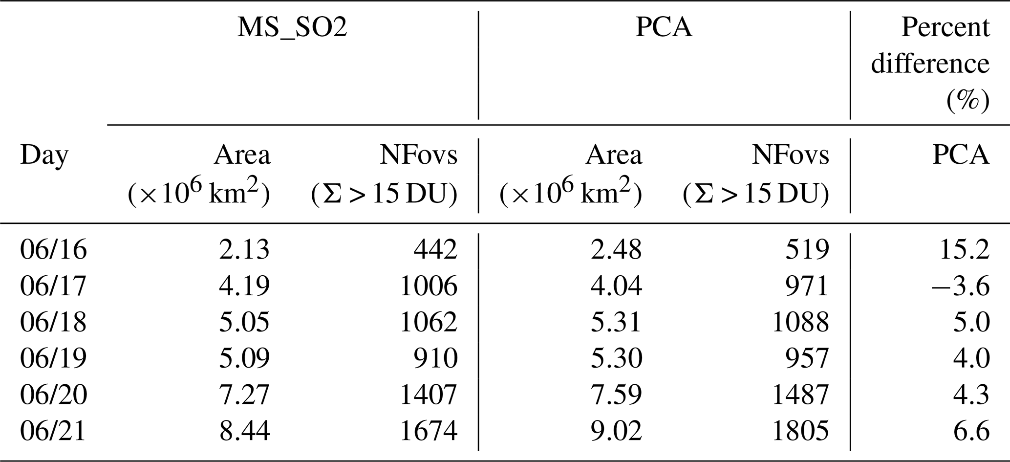
Table 4 provides estimates of the plume area for the MS_SO2 and PCA. The area of the plume is most sensitive to the minimum detection threshold around the edges of the SO2 cloud. MS_SO2 and the PCA algorithms were directly compared by computing the areal sum of all the pixels where Σ > 15 DU (Fig. 9). For the 6 d study period, the plume increased in size from about a little over 2×10⁶ km2 to km2 The PCA trends observed a larger cloud area for five of the 6 d, with most of the observed differences within 7 %. On 16 June, shortly after the major eruption of 15 June, the estimated area for the PCA is about 15 % greater than for MS_SO2. The fresh plumes are opaque, which result in underestimating of SO2 mass by all BUV algorithms due to the mixing of aerosols (Krotkov et al., 1997). The PCA appears slightly more sensitive to SO2 near the edges of the cloud, where aerosol loading is high (AI > 1.5). It should be noted that the soft calibration applied to the 340 nm channel, described in Sects. 3.3 and S3.3, may also contribute to the lowering the sensitivity around the edges of the plume. This correction effectively lowered the background by about 3 DU.
This paper describes a discrete multi-satellite UV wavelength algorithm (MS_SO2) for retrieving volcanic SO2 that was used operationally to process measurements from the heritage Nimbus-7 TOMS and the Deep Space Climate Observatory Earth Polychromatic Imaging Camera (Carn et al., 2018; Marshak et al., 2018). The MS_SO2 algorithm retrieves four parameters (SO2, O3, dR∕dλ and Rs) and can be used to process data from current hyperspectral UV spectrometers, such as SNPP/OMPS and Aura/OMI, using a convolved, discrete set of wavelengths, offering a viable means for intercomparing volcanic SO2 retrievals from different missions.
We estimated random (noise) and systematic errors, related to the effects of volcanic aerosols and uncertainties in SO2 height and partly corrected for absorbing ash, using positive aerosol index (AI) as a proxy for applying a Step 2 correction to the SO2 retrievals. The correction could still underestimate SO2 mass during the first days after extremely large eruptions (VEI > 3) due to BUV saturation. In such cases we recommend estimating e-folding time of the SO2 decay, using later measurements and extrapolating SO2 mass exponentially back in time to the eruption day (Krotkov et al., 2010).
The TOMS Observing System Simulation Experiment simulation, using synthetic radiances, shows unbiased MS_SO2 retrievals of for SO2 < 100–150 DU but low biases for larger SO2 amounts due to the presence of ash and sulfate aerosols. Therefore, operational MS_SO2 retrievals should provide a low boundary constraint on the SO2 mass injected into the atmosphere from large eruptions during first days after an eruption. The algorithm can be further improved by explicitly accounting for volcanic ash and sulfate aerosols, which was not feasible in the operational processing.
The MS_SO2 retrieval is also sensitive to differences between the a priori and actual SO2 center of mass altitude. Since this key parameter is not retrieved, the TOMS SO2 product provides separate SO2 column amounts assuming three different SO2 altitudes (8, 13 and 18 km). Users should base their analysis on the altitude that is most appropriate for a particular eruption.
To assess the overall accuracy of the TOMS SO2 retrievals, we compared MS_SO2 and independent PCA algorithms for the first 6 d following the 1991 Pinatubo eruption. The daily time series of SO2 retrievals showed high correlation (R2=0.986) and excellent agreement between the two retrievals over a broad SO2 range between 15 and 400 DU. We also compared the SO2 mass, peak SO2 amounts and plume area with the heritage Krueger–Kerr algorithm. This three-way comparison showed the SO2 mass within 10 % for all days, except on 16 June, when the Krueger–Kerr algorithm retrieved 24 % higher SO2 mass. This could be explained by interpolation over a region of missing TOMS measurements on 16 June (Guo et al., 2004). The remaining differences between current MS_SO2 and the PCA algorithms (3 %–7 %) are attributed to the differences in handling of aerosols and different sensitivity thresholds of the algorithms.
The reprocessed Nimbus-7 TOMS volcanic SO2 data set (TOMSN7SO2) is now publicly available through the Goddard Earth Sciences Data and Information Services Center (GES DISC) as part of the NASA's Making Earth System Data Records for Use in Research Environments (MEaSUREs) program (Krotkov et al., 2019). We plan to reprocess all follow-up multispectral UV (TOMS) and hyperspectral UV (OMI, OMPS) missions (Fig. 1) with MS_SO2 and PCA algorithms to keep updating our multi-satellite volcanic SO2 mass database archived at GES DISC (Carn, 2019). It is important to continue quantifying SO2 emissions from small explosive eruptions, as they may, collectively, play an important role in sustaining the persistent, background stratospheric aerosol layer, which is an important factor in global climate forcing.
Our data can be publicly accessed at https://disc.gsfc.nasa.gov/datasets/TOMSN7SO2_3/summary?keywords=TOMS SO2 (Krotkov et al., 2019).
The supplement related to this article is available online at: https://doi.org/10.5194/amt-12-5137-2019-supplement.
BF implemented the MS_SO2 algorithm, processed and archived the N7TOMS SO2 data record, wrote most of the text and supplement, produced the figures, and coordinated with the other co-authors. NK advised on paper organization and figures and wrote Sect. 2.2 and the Conclusion. PB developed the theoretical basis for the MS_SO2 algorithm and wrote Sect. 2.1 on the heritage ozone algorithm. CL provided PCA SO2 results and contributed to Sects. 4.2 and 5 and the Supplement. SC wrote the Introduction and important scientific analysis of the data. EH contributed to Sect. 4.2.2, quantifying the effects of ash and sulfate aerosols on the MS_SO2 retrieval. PL proposed and implemented the data format used in the MEaSUREs archived SO2 products.
The authors declare that they have no conflict of interest.
This work was supported by NASA's Making Earth System data records for Use in Research Environments (NNH12ZDA001N-MEASURES) program. Can Li acknowledges support from NASA Earth Science Division for development and analysis of hyperspectral PCA SO2 products for OMPS (grant no. 80NSSC18K0688). Eric Hughes was supported by NASA grant to the University of Maryland no. NNX13AG51G. Simon A. Carn acknowledges support from NASA grant NNX13AF50G.
This paper was edited by Michel Van Roozendael and reviewed by two anonymous referees.
Ahmad, Z. and Bhartia, P. K.: Effect of Molecular anisotropy on the backscattered UV radiance, Appl. Optics, 34, 8309–8314, https://doi.org/10.1364/AO.34.008309, 1995.
Ahmad, Z., Bhartia P. K., and Krotkov, N. A.: Spectral properties of backscattered UV radiation in cloudy atmospheres, J. Geophys. Res.-Atmos., 109, D01201, https://doi.org/10.1029/2003JD003395, 2004.
Bhartia, P. K. (Ed.): OMI Algorithm Theoretical Basis Document, Vol. II, Ozone Products, available at: https://disc.gsfc.nasa.gov/datasets/OMTO3_V003/summary?keywords=OMTO3 (last access: 11 September 2019), 2002.
Bobrowski, N., Honninger, G., Galle, B., and Platt, U.: Detection of bromine monoxide in a volcanic plume, Nature, 423, 273–276, http://https://doi.org/10.1038/nature01625, 2003.
Bogumil, K., Orphal, J., Homann, T., Voigt, S., Spietz, P., Fleischmann, O. C., Vogel, A., Hartmann, M. Kromminga, H., Bovensmann, H., Frerick, J., Burrows J. P.: Measurements of molecular absorption spectra with the SCIAMACHY pre-flight model: instrument characterization and reference data for atmospheric remote-sensing in the 230–2380 nm region, J. Photoch. Photobio. A, 157, 167–184, https://doi.org/10.1016/S1010-6030(03)00062-5, 2003.
Bluth, J. S. G., Doiron, S. D., Schnetzler, C. C., Krueger, A. J., and Walter, L. S.: Global tracking of the SO2 clouds from the June, 1991 Mount Pinatubo eruptions, Geophys. Res. Lett., 19, 151–154, https://doi.org/10.1029/91GL02792, 1992.
Buchard, V., Randles, C. A., da Silva, A., Darmenov, A. S., Colarco, P. R., Govindaraju, R. C., Ferrare, R. A., Hair, J. W., Beyersdorf, A., Ziemba, L. D., and Yu, H.: The MERRA-2 Aerosol Reanalysis, 1980–onward, Part II: Evaluation and Case Studies, J. Climat, 30, 6851–6872, https://doi.org/10.1175/JCLI-D-16-0613.1, 2017.
Carn, S. A.: Multi-Satellite Volcanic Sulfur Dioxide L4 Long-Term Global Database V3, Greenbelt, MD, USA, Goddard Earth Science Data and Information Services Center (GES DISC), https://doi.org/10.5067/MEASURES/SO2/DATA404, 2019.
Carn, S. A., Krueger, A. J., Bluth, G. J. S., Schaefer, S. J., Krotkov, N. A., Watson, I. M., and Datta, S.: Volcanic eruption detection by the Total Ozone Mapping Spectrometer (TOMS) instruments: a 22-year record of sulfur dioxide and ash emissions, in: Volcanic Degassing, edited by: Oppenheimer, C., Pyle, D. M., and Barclay, J., Geological Society, London, Special Publications, 213, 177–202, https://doi.org/10.1144/GSL.SP.2003.213.01.11, 2003.
Carn, S. A., Yang, K., Prata, A. J., and Krotkov, N. A.: Extending the long-term record of volcanic SO2 emissions with the Ozone Mapping and Profiler Suite (OMPS) Nadir Mapper, Geophys. Res. Lett., 42, 925–932, https://doi.org/10.1002/2014GL062437, 2015.
Carn, S. A., Clarisse, L., and Prata, A. J.: Multi-decadal satellite measurements of global volcanic degassing, J. Volcanol. Geoth. Res., 311, 99–134, https://doi.org/10.1016/j.jvolgeores.2016.01.002, 2016.
Carn, S. A., Krotkov, N. A. Fisher, B. L., Li, C., and Prata, A. J.: First observations of volcanic eruption clouds from the L1 Earth-Sun Lagrange point by DSCOVR/EPIC, Geophys. Res. Lett., 45, 11456–11464, https://doi.org/10.1029/2018GL079808, 2018.
Chin, M., Rood, R. B., Lin, S., and Muller, J. F.: Atmospheric sulfur cycle simulated in the global model GOCART: Model description and global properties, J. Geophys. Res.-Atmos., 105, 24671–24688, https://doi.org/10.1029/2000JD900384, 2000.
Colarco, P., Da Silva, A., Chin, M., and Dielh, T.: Online simulations of global aerosol distributions in the NASA GEOS‐4 model and comparisons to satellite and ground-based aerosol optical depth, J. Geophys. Res.-Atmos., 115, D14207, https://doi.org/10.1029/2009JD012820, 2010.
Colarco, P., Nowottnick, E. P., Randles, C. A., Yi, B., Yang, P., Kim, K., Smith, J. A., and Bardeen, C. G.: Impact of radiatively interactive dust aerosols in the NASA GEOS-5 climate model: Sensitivity to dust particle shape and refractive index, J. Geophys. Res.-Atmos., 119, 753–786, https://doi.org/10.1002/2013JD020046, 2014.
Colarco, P. R., Gassó, S., Ahn, C., Buchard, V., da Silva, A. M., and Torres, O.: Simulation of the Ozone Monitoring Instrument aerosol index using the NASA Goddard Earth Observing System aerosol reanalysis products, Atmos. Meas. Tech., 10, 4121–4134, https://doi.org/10.5194/amt-10-4121-2017, 2017.
Daumont, M., Brion, J., Charbonnier, J., and Malicet, J.: Ozone UV spectroscopy I: Absorption cross-sections at room temperature, J. Atmos. Chem., 15, 145–155, https://doi.org/10.1016/j.jvolgeores.2016.01.002, 1992.
Dave, J. D.: Meaning of successive iteration of the auxiliary equation in the theory of radiative transfer, Astrophys. J., 140, 1292–1303, https://doi.org/10.1086/148024, 1964.
Dave, J. V.: Effect of aerosols on the total ozone in an atmospheric column from measurements of its ultraviolet radiance, J. Atmos. Sci., 35, 899–911, https://doi.org/10.1175/1520-0469(1978)035<0899:EOAOTE>2.0.CO;2, 1978.
Dave, J. V. and Mateer, C. L.: A preliminary study on the possibility of estimating total atmospheric ozone from satellite measurements, J. Atmos. Sci., 24, 414–427, https://doi.org/10.1175/1520-0469(1967)024<0414:APSOTP>2.0.CO;2, 1967.
Guo, S., Bluth, G. J. S., Rose, W. I., Watson, I. M., and Prata, A. J.: Revaluation of SO2 release of the 15 June 1991 Pinatubo eruption using ultraviolet and infrared satellite sensors, Geochem. Geophy. Geosy., 5, 1–31, Q04001, https://doi.org/10.1029/2003GC000654, 2004.
Joiner, J., Bhartia, P. K., Cebula, R. P., Hilsenrath, E., McPeters, R. D., and Park, H. W.: Rotational-Raman Scattering (Ring Effect) in satellite backscatter ultraviolet measurements, Appl. Optics 34, 4513–4525, https://doi.org/10.1364/AO.34.004513, 1995.
Kern, C., Sihler, H., Vogel, L., Rivera, C., Herrera, M., and Platt, U.: Halogen oxide measurements at Masaya volcano, Nicaragua using active long path differential optical absorption spectroscopy, B. Volcanol., 71, 659–670, https://doi.org/10.1007/s00445-008-0252-8, 2009.
Kerr, J. B., McElroy, C. T., and Olafson, R. A.: Measurements of ozone with the Brewer ozone spectrophotometer, Proc. Int. Ozone Symp., 1, 74–79, https://doi.org/10.1029/94JD02147, 1980.
Klenk, K. F., Bhartia, P. K., Hilsenrath E., and Fleig, A. J.: Standard Ozone Profiles from Balloon and Satellite Data Sets, J. Clim. Appl. Meteorol., 22, 2012–2022, https://doi.org/10.1175/1520-0450(1983)022<2012:SOPFBA>2.0.CO;2, 1983.
Khokhar, M. F., Frankenberg, C., Van Roozendael, M., Beirle, S., Kühl, S., Richter, A., Platt, U., and Wagner, T.: Satellite observations of atmospheric SO2 from volcanic eruptions during the time-period of 1996–2002, Adv. Space Res. 36, 879–887, https://doi.org/10.1016/j.asr.2005.04.114, 2002.
Klobas, J. E., Wilmouth, D. M., Weisenstein, D. K., Anderson, J. G., and Salawitch, R. J.: Ozone depletion following future volcanic eruptions, Geophys. Res. Lett., 44, 7490–7499, https://doi.org/10.1002/2017GL073972, 2017.
Krotkov, N. A., Krueger, A. J., and Bhartia, P. K.: Ultraviolet optical model of volcanic clouds for remote sensing of ash and sulfur dioxide, J. Geophys. Res., 102, 21891–21904, https://doi.org/10.1029/97JD01690, 1997.
Krotkov, N. A., Carn, S. A., Krueger, A. J., Bhartia, P. K., and Yang, K.: Band residual difference algorithm for retrieval of SO2 from the Aura Ozone Monitoring Instrument (OMI), IEEE T. Geosci. Remote, 44, 1259–1266, https://doi.org/10.1109/TGRS.2005.861932, 2006.
Krotkov, N. A., Schoeberl, M., Morris, G., Carn, S., and Yang, K.: Dispersion and lifetime of the SO2 cloud from the August 2008 Kasatochi eruption, J. Geophys. Res., 115, D00L20, https://doi.org/10.1029/2010JD013984, 2010.
Krotkov, N. A., Bhartia, P. K., Fisher, B., and Leonard P.: TOMS/N7 MS SO2 Vertical Column 1-Orbit L2 Swath 50x50 km V3, Greenbelt, MD, USA, Goddard Earth Sciences Data and Information Services Center (GES DISC), https://doi.org/10.5067/MEASURES/SO2/DATA204, 2019.
Krueger, A. J.: Sighting of El Chichón sulfur dioxide clouds with the Nimbus 7 total ozone mapping spectrometer, Science, 220, 1377–1379, https://doi.org/10.1126/science.220.4604.1377, 1983.
Krueger, A. J., Walter, L. S., Bhartia, P. K., Schnetzler, C. C., Krotkov, N. A., Sprod, I., and Bluth, G. J. S.: Volcanic sulfur dioxide measurements from the total mapping spectrometer instruments, J. Geophys. Res., 100, 14057–14076, https://doi.org/10.1029/95JD01222, 1995.
Krueger, A. J., Schaefer, S. J., Krotkov, N. A., Bluth, G. J. S., and Barker, S.: Ultraviolet remote sensing of volcanic emissions, in Remote Sensing of Active Volcanism, Geophys. Monogr. Ser., 116, edited by: Mouginis-Mark, P. J., Crisp, J. A., and Fink, J. H., 25–43, https://doi.org/10.1029/GM116p0025, 2000.
Krueger, A. J., Krotkov, N. A., and Carn, S. A.: El Chichon: the genesis of volcanic sulfur dioxide monitoring from space, J. Volcanol. Geoth. Res., 175, 408–414, https://doi.org/10.1016/j.jvolgeores.2008.02.026, 2008.
Lee, C., Richter, A., Weber, M., and Burrows, J. P.: SO2 Retrieval from SCIAMACHY using the Weighting Function DOAS (WFDOAS) technique: comparison with Standard DOAS retrieval, Atmos. Chem. Phys., 8, 6137–6145, https://doi.org/10.5194/acp-8-6137-2008, 2008.
Li, C., Joiner, J., N. A. Krotkov, and Bhartia, P. K.: A fast and sensitive new satellite retrieval algorithm based on principal component analysis: application to the ozone monitoring instrument, Geophys. Res. Lett., 40, 6314–6318, https://doi.org/10.1002/2013gl058134, 2013.
Li, C., Krotkov, N. A., Carn, S., Zhang, Y., Spurr, R. J. D., and Joiner, J.: New-generation NASA Aura Ozone Monitoring Instrument (OMI) volcanic SO2 dataset: algorithm description, initial results, and continuation with the Suomi-NPP Ozone Mapping and Profiler Suite (OMPS), Atmos. Meas. Tech., 10, 445–458, https://doi.org/10.5194/amt-10-445-2017, 2017.
Mankin, W. G. and Coffey, M. T.: Increased stratospheric hydrogen chloride in the El Chichón cloud, Science, 226, 170–172, https://doi.org/10.1126/science.226.4671.170, 1984.
Marshak, A., Herman, J., Szabo, A., Blank, K., Carn, S., Cede, A., Geogdzhayev, I., Huang, D. Huang, L., Knyazikhin, Y., Kowalewski, M., Krotkov, N., Lyapustin, A., McPeters, R., Meyer, K. G., Torres, O., and Yang, Y.: Earth observations from DSCOVR/EPIC instrument, B. Am. Meteorol. Soc., 99, 1829–1850, https://doi.org/10.1175/BAMS-D-17-0223.1, 2018.
Mateer, C. L., Heath, D. F., and Krueger, A. J.: Estimation of Total Ozone from Satellite Measurements of Backscattered Ultraviolet Earth Radiance, J. Atmos. Sci., 28, 1307–1311, https://doi.org/10.1175/1520-0469(1971)028<1307:EOTOFS>2.0.CO;2, 1971.
McPeters, , R. D., Bhartia, P. K., Kureger, A. J., and Herman, J. R.: Nimbus-7 Total Ozone Mapping Spectrometer (TOMS) Data Products User's Guide, NASA Reference Publication 1384, 1996.
Molod, A., Takacs, L., Suarez, M., Bacmeister, J., Song, I. S., and Eichmann, A.: The GEOS-5 Atmospheric General Circulation Model: Mean Climate and Development from MERRA to Fortuna, Technical Report Series on Global Modeling and Data Assimilation, 28, 2012.
Prata, A. J., Rose, W. I., Self, S., and O'Brien, D. M.: Global, long-term sulphur dioxide measurements from TOVS data: A new tool for studying explosive volcanism and climate, in Volcanism and the Earth's Atmosphere, Geophys. Monogr. Ser., vol. 139, AGU, Washington, DC, edited by: Robock, A. and Oppenheimer, C., 75–92, https://doi.org/10.1029/139GM05, 2003.
Ridley, D. A., Solomn, S., Barnes, J. E., Burlakov, V. D., Deshler, T., Dolgil, S. I., Herber, A. B., Nagai, T., Neely III, R. R., Nevzorov, A. V., Ritter, C., Sakai, T., Santer, B. D., Sato, M., Schmidt, A., Uchino, O., and Vernier, J. P: Total volcanic stratospheric aerosol optical depths and implications for global climate change, Geophys. Res. Lett., 41, 7763–7769, https://doi.org/10.1002/2014GL061541, 2014.
Robock, A.: Volcanic eruptions and climate, Rev. Geophys., 38, 191–219, https://doi.org/10.1029/1998RG000054, 2000.
Rose, W. I., Gu, Y., Watson, I. M., Yu, T., Bluth, G. J. S., Prata, A. J., Krueger, A. J., Krotkov, N., Carn, S., Fromm, M. D., Hunton, D. E., Viggiano, A. A., Miller, T. M., Ballentin, J. O., Ernst, G. G. J., Reeves, J. M., Wilson, C., and Anderson, B. E.: The February–March 2000 eruption of Hekla, Iceland from a satellite perspective, in: Volcanism and the Earth's Atmosphere, edited by: Robock A. and Oppenheimer, C., AGU Geophysical Monograph 139, 107–132, 2003.
Self, S., Zhao, J.-X., Holasek, R. E., Torres, R. C., and King, A. J.: The atmospheric impact of the Mount Pinatubo eruption, in: Fire and Mud: Eruptions and lahars of Mount Pinatubo, Philippines, edited by: Newhall, C. G. and Punongbayan, R. S., Philippine Institute of Volcanology and Seismology, Quezon City, and University of Washington Press, Seattle, 1089–1115, 1996.
Solomon, S., Portmann, R. W., Garcia, W., Randel, R. R., Wu, F., Nagatani, R., Gleason, J., Thomason, L., Poole, L. R., and McCormick, M. P.: Ozone Depletion at mid-latitudes: coupling of volcanic aerosols and temperature variability to anthropogenic chlorine, Geophys. Res. Lett., 25, 1871–1874, https://doi.org/10.1029/98GL01293, 1998.
Solomon, S., Daniel, J. S., Neely III, R. R., Vernier, J. P., Dutton, E. G., and Thomason, L. W.: The persistently variable “background” stratospheric aerosol layer and global climate change, Science, 333, 866–870, https://doi.org/10.1126/science.1206027, 2011.
Spurr, R.: LIDORT and VLIDORT: Linearized pseudo-spherical scalar and vector discrete ordinate radiative transfer models for use in remote sensing retrieval problems, in: Light Scattering Reviews 3, edited by: Kokhanovsky, A. A., Springer Praxis Books, Springer, Berlin, Heidelberg, https://doi.org/10.1007/978-3-540-48546-9_7, 2008.
Theys, N., De Smedt, I., van Gent, J., Danckaert, T., Wang, T., Hendrick, F., Stavrakou, T., Bauduin, S., Clarisse, L., Li, C, Krotkov, N. A., Yu, H., Benot, H., and Van Roozendael, M.: Sulfur dioxide vertical column DOAS retrievals from the Ozone Monitoring Instrument: Global observations and comparison to ground-based and satellite data, J. Geophys. Res.-Atmos., 120, 2470–2491, https://doi.org/10.1002/2014JD022657, 2015.
Toon, O. B., Turco, R. P., Westphal, D., Malone, R., and Liu, M. S.: A multidimensional model for aerosols: Description of computational analogs, J. Atmos. Sci., 45, 2123–2143, https://doi.org/10.1175/1520-0469(1988)045<2123:AMMFAD>2.0.CO;2, 1988.
Veefkind, J. P., Aben, I., McMullan, K., Förster, H., de Vries, J., Otter, G., Claas, J., Eskes, H. J., de Haan, J. F., Kleipool, Q., van Weele, M., Hasekamp, O., Hoogeveen, R., Landgraf, J., Snel, R., Tol, P., Ingmann, P., Voors, R., Kruizinga, B, Vink R., Visser, H., and Levelt, P. F.: TROPOMI on the ESA Sentinel-5 Precursor: A GMES mission for global observations of the atmospheric composition for climate, air quality and ozone layer applications, Remote Sens. Environ., 120, 70–83, https://doi.org/10.1016/j.rse.2011.09.027, 2012.
Vernier, J. P., Thomason, L. W., Pommereau, J. P., Bourassa, A., Pelon, J., Garnier, A., Hauchecorne, A., Blanot, L., Trepte, C., Degenstein., D., and Vargas, F.: Major influence of tropical volcanic eruptions on the stratospheric aerosol layer during the last decade, Geophys. Res. Lett. 38, L12807, https://doi.org/10.1029/2011GL047563, 2011.
Yang, K., Krotkov, N. A., Krueger, A. J., Carn, S. A., Bhartia, P. K., and Levelt, P. F.: Retrieval of large volcanic SO2 columns from the AuraOzone Monitoring Instrument: Comparison and limitations, J. Geophys. Res., 112, D24S43, https://doi.org/10.1029/2007JD008825, 2007.
Yang, K., Liu, X., Bhartia, P. K., Krotkov, N. A., Carn, S. A., Hughes, E., Krueger, A. J., Spurr R., and Trahan S.: Direct Retrieval of Sulfur Dioxide Amount and Altitude from Spaceborne Hyper-spectral UV Measurements: Theory and Application, J. Geophys. Res., 115, D00L09, https://doi.org/10.1029/2010JD013982, 2010.
Zhang, Y., Li, C., Krotkov, N. A., Joiner, J., Fioletov, V., and McLinden, C.: Continuation of long-term global SO2 pollution monitoring from OMI to OMPS, Atmos. Meas. Tech., 10, 1495–1509, https://doi.org/10.5194/amt-10-1495-2017, 2017.