the Creative Commons Attribution 4.0 License.
the Creative Commons Attribution 4.0 License.
 | 01 Oct 2019
Quantifying CH4 emissions from hard coal mines using mobile sun-viewing Fourier transform spectrometry
Ralph Kleinschek
Leon Scheidweiler
Sara Defratyka
Mila Stanisavljevic
Andreas Forstmaier
Alexandru Dandocsi
Sebastian Wolff
Darko Dubravica
Norman Wildmann
Julian Kostinek
Patrick Jöckel
Anna-Leah Nickl
Theresa Klausner
Frank Hase
Matthias Frey
Florian Dietrich
Jarosław Nȩcki
Justyna Swolkień
Andreas Fix
Anke Roiger
André Butz
Methane (CH4) emissions from coal production amount to roughly one-third of European anthropogenic CH4 emissions in the atmosphere. Poland is the largest hard coal producer in the European Union with the Polish side of the Upper Silesian Coal Basin (USCB) as the main part of it. Emission estimates for CH4 from the USCB for individual coal mine ventilation shafts range between 0.03 and 20 kt a−1, amounting to a basin total of roughly 440 kt a−1 according to the European Pollutant Release and Transfer Register (E-PRTR, http://prtr.ec.europa.eu/, 2014). We mounted a ground-based, portable, sun-viewing FTS (Fourier transform spectrometer) on a truck for sampling coal mine ventilation plumes by driving cross-sectional stop-and-go patterns at 1 to 3 km from the exhaust shafts. Several of these transects allowed for estimation of CH4 emissions based on the observed enhancements of the column-averaged dry-air mole fractions of methane (XCH4) using a mass balance approach. Our resulting emission estimates range from 6±1 kt a−1 for a single shaft up to 109±33 kt a−1 for a subregion of the USCB, which is in broad agreement with the E-PRTR reports. Three wind lidars were deployed in the larger USCB region providing ancillary information about spatial and temporal variability of wind and turbulence in the atmospheric boundary layer. Sensitivity studies show that, despite drawing from the three wind lidars, the uncertainty of the local wind dominates the uncertainty of the emission estimates, by far exceeding errors related to the XCH4 measurements themselves. Wind-related relative errors on the emission estimates typically amount to 20 %.
- Article
(4419 KB) - Full-text XML
- BibTeX
- EndNote


Atmospheric methane (CH4) causes the second largest radiative forcing of the long-lived greenhouse gases after carbon dioxide (IPCC, 2013). Except for the period from about 1999 to 2006, the global atmospheric CH4 burden has been rising since 1750 and is now a factor of roughly 1.5 higher than in the pre-industrial era (Nisbet et al., 2014; Miller et al., 2013). Reasons for the renewed rise since 2007 are debated. Increased anthropogenic emissions are likely to be part of the answer (Bousquet et al., 2006; Kirschke et al., 2013; Schwietzke et al., 2016; Nisbet et al., 2016; Helmig et al., 2016; Worden et al., 2017).
Generally, about 20 % of the global methane source is thought to be caused by the fossil fuel industry (Schwietzke et al., 2016; Bousquet et al., 2006). The E-PRTR (European Pollutant Release and Transfer Register, http://prtr.ec.europa.eu/, 2014) reports the total European anthropogenic CH4 emission as 1874 kt for the year 2014. Methane emitted by underground mining and related operations amounts to 686 kt a−1 for all reporting facilities in Europe. With emissions of 466 kt a−1 the Upper Silesian Coal Basin (USCB) in Poland is a CH4-emitting hotspot in Europe. The USCB roughly comprises an area of 50 km×50 km centred at 50.1∘ N, 18.8∘ E with about 50 active CH4 ventilating hard coal mining shafts emitting between 0.03 and 20 kt a−1 (E-PRTR, 2014). The USCB was the main target of the CoMet (Carbon dioxide and Methane mission 2018) campaign, which covered roughly 3 weeks from 23 May to 12 June 2018. During CoMet several aircraft and ground-based instruments were co-deployed to evaluate strategies on how to verify the local CH4 emissions. Here, we focus on the CoMet measurements of a single mobile ground-based, sun-viewing FTS.
The sun-viewing FTS of the type EM27/SUN developed by the Karlsruhe Institute of Technology in collaboration with Bruker Optics (Gisi et al., 2012) is generally used to measure the column-averaged dry-air mole fractions of methane (XCH4) and other gases by measuring direct-sun absorption spectra in the shortwave-infrared spectral range (around 6000 cm−1). Recently, Hase et al. (2015) and Chen et al. (2016) combined several of these FTS instruments into ad hoc networks in the vicinity of major cities to estimate urban carbon dioxide (CO2) and CH4 emissions respectively. Viatte et al. (2017) used a similar FTS configuration together with large-eddy simulations to estimate the amount of CH4 emitted by dairies in southern California. Toja-Silva et al. (2017) verified power plant emissions with computational fluid dynamics simulations and differential column measurements using two EM27/SUN instruments in Munich. Klappenbach et al. (2015) demonstrated mobile deployment on a research vessel requiring a custom-built solar tracker to compensate for the motion of the platform. Butz et al. (2017) mounted the EM27/SUN on a small truck to measure the volcanic CO2 plume of Mt. Etna by recording plume transects in stop-and-go patterns. Kille et al. (2019) separated natural from agricultural CH4 emissions using a network of four EM27/SUN instruments.
Based on a mobile FTS setup similar to Butz et al. (2017), we explore the feasibility of estimating CH4 emissions for individual coal mine ventilation shafts and groups of shafts. To this end, we mounted the EM27/SUN on a truck and we drove transects through the CH4 plumes in the USCB while driving in stop-and-go patterns. We estimated emissions from the recorded XCH4 enhancements using a mass balance method, which was assisted by wind information from three wind lidars deployed in the broader region. Section 2 summarizes the campaign setup, describes the deployed instruments and the data analysis, and explains the emission estimation method. Emission estimates of CH4 are summarized in Sect. 3 followed by the analysis of the errors in Sect. 4. We evaluate the suitability of the method used, compare the estimated emissions to the E-PRTR database, and conclude this work with Sect. 5.
Figure 1 shows a map of the USCB. The coal mine ventilation shafts group into a northern part in the vicinity of the city of Katowice and into a southern part close to the Czech border. The reported operations of the mobile FTS were carried out in the southern part where the largest emitters are expected. In the framework of CoMet, we also operated three wind lidars and four stationary, sun-viewing FTS of the same model as the mobile one at stations surrounding the USCB. In situ sensors were deployed in cars sampling throughout the region. Aircraft carrying in situ (Kostinek et al., 2019) and remote sensing instrumentation (Gerilowski et al., 2011) were operated out of Katowice airport, and a long-distance aircraft (Amediek et al., 2017) visited the USCB operating out of the airport at Oberpfaffenhofen close to Munich, Germany.
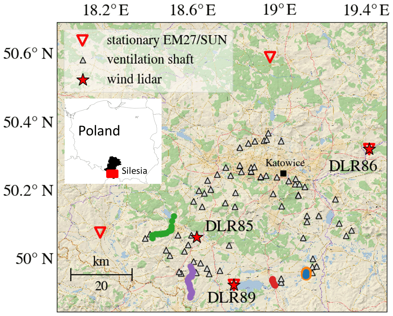
Figure 1Map of the USCB in southern Poland (see small inset on the left with black illustrating the region of Silesia and red depicting the map excerpt of the USCB). Ventilation shafts are grey triangles. Coloured dots depict five plume transects measured using the mobile FTS on 24 May at around 07:00–08:00 UTC (UTC used for all times throughout the paper, orange), on 24 May around noon (blue), on 1 June (green), on 6 June during morning hours (red), and on 6 June around noon (purple). The most active CH4 emitters are assumed to be located in the southern part of the USCB, which is why mobile FTS measurements are focused on this area. Stationary EM27/SUN FTS locations are marked as red triangles; the three wind lidars DLR85, DLR86, and DLR89 are marked as red stars. Eastern and southern wind lidars are placed at the same locations as the respective EM27/SUNs. Background map from ESRI (2019).
Here, we use the mobile FTS measurements (Sect. 2.1) and the wind lidar data (Sect. 2.2) together with the cross-sectional flux method (Sect. 2.3) to estimate CH4 emissions. Future studies will target the other CoMet data and aim at combining them.
2.1 Mobile FTS observatory
The mobile FTS observatory consists of a Bruker EM27/SUN Fourier transform spectrometer with a custom-built solar tracker deployed on a truck similar to the setup used by Butz et al. (2017). The custom-built solar tracker enables efficient stop-and-go patterns since it supports start-up and repointing within a few seconds once the solar tracking is interrupted. During driving, however, significant high-frequency mechanical disturbances occur, which is not yet compensated for by the tracker. The mobile FTS observatory was operated out of its campaign-base at the site Pustelnik in the south of the USCB between 23 May and 12 June 2018 whenever weather conditions were promising for direct sun viewing. The mobile instrument followed public roads on approximately perpendicular tracks to the assumed plume 1 to 3 km downwind of the targeted CH4 sources (Fig. 1). We chose the transects depending on the wind direction and aimed for isolated shafts with preferably no other shafts upwind. However, we also examined subregions within the USCB containing several mines and shafts upwind. For the plume transects, it was necessary to sample the CH4 background on both sides of the plume in order to reliably remove the XCH4 background and to derive the above-background enhancements, which are used for the emission estimation. In total, we report on five transects. One morning transect and one noon transect for 24 May, one transect on 1 June, and one morning transect and one noon transect on 6 June.
The EM27/SUN used here has a spectral resolution of 0.5 cm−1 and operates in the spectral range of 4000 to 11 000 cm−1. Frey et al. (2019) observed an average instrument-to-instrument difference of 0.8 ppb for XCH4 for an ensemble of instruments. According to the Allan deviations described by Chen et al. (2016) the precision of XCH4 for 120 s integration time is 0.3 ppb, which is roughly 0.02 % of the total column. The accuracy amounts to roughly 4.7 ppb based on 3 h side-by-side measurements with the Karlsruhe TCCON station in spring 2017. We recorded double-sided interferograms with a sampling rate of 10 kHz and we typically co-added 10 double-sided interferograms resulting in roughly 120 s total integration time per stop. Typical dwell times per stop in our stop-and-go patterns were 2 min 30 s. For the last part of our deployment on 6 June we increased the sampling rate to 40 kHz, which resulted in average dwell times of 60 s. As depicted in Fig. 2 the FTS is mounted on a suspension plate. The rubber bearings absorb minor shocks and protect the instrument from major bumps. A 12 V battery powers the whole system. We remotely operated the instrument from inside the driver's cabin, which enabled us to measure alongside busy roads as we did not have to leave the car to start the measurements. The solar tracker is the standard two-mirror system developed by Gisi et al. (2011) supplemented with a two-stage tracking control mechanism. The coarse tracking stage uses a fish-eye camera that identifies the position of the sun and gears the tracker into the vicinity of the sun. The fine-tracking system is the camera system developed by Gisi et al. (2011), which takes over once the coarse tracking is successful. Generally, the fine-tracking errors amount to 10 arcsec; i.e. the tracking is precise to within fractions of the apparent diameter of the solar disk.
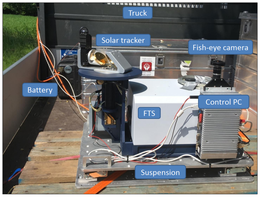
Figure 2Mobile FTS (EM27/SUN) mounted on a truck. Direct sunlight is collected via the solar tracker. The battery supplies the measurement notebook inside the vehicle, the spectrometer including the solar tracker, and the control PC. A fish-eye camera automatically detects the solar disc in the sky above the spectrometer. The control PC steers the solar tracker towards the solar disc.
For the retrieval of XCH4 from the FTS measurements we use the software package PROFFIT (Hase et al., 2004), which is in routine use for accurate trace gas retrievals from shortwave-infrared direct-sun absorption spectra (e.g. Gisi et al., 2012; Frey et al., 2015; Klappenbach et al., 2015; Chen et al., 2016; Butz et al., 2017; Frey et al., 2019). Quality filtering, based on the unmodulated (DC) part of the recorded interferograms, removes all measurements that are affected by unstable pointing conditions, e.g. due to intermittent thin clouds disturbing solar tracking (e.g. Klappenbach et al., 2015). We set the DC fluctuation threshold to 1 % for discarding corrupt interferograms. The spectral bandwidth of the EM27/SUN allows for measurements of H2O, O2, CO2, CH4, CO (CO in combination with an additional channel described by Hase et al. (2016)), and other gases if present in significant amounts (Butz et al., 2017). Related species for this study are O2 and CH4. The spectral retrieval windows for these target absorbers are 7765 to 8005 and 5897 to 6145 cm−1 for O2 and CH4 respectively. The absorption line parameters are taken from Toon (2017) and Rothman et al. (2009). Assuming that the targeted CH4 plumes mainly reside in the planetary boundary layer (PBL), the PROFFIT retrieval was set up to estimate the total column of methane (CH4), in units of molecules per square metre, by only scaling the lower part (<1700 m a.g.l.) of the a priori vertical profile taken from the EMAC model. Following Butz et al. (2017), who only scaled the relevant plume layers of mount Etna in Sicily, we only scaled the relevant layers of the CH4 plumes. Here, we use EMAC simulation results from a simulation similar to the simulation described by Jöckel et al. (2016). Figure A1 compares CH4 profiles of both a priori and retrieved CH4 columns, which are congruent above 1700 m a.g.l.
For the O2 retrieval we scaled the full a priori profile. The column-averaged dry-air mole fraction of methane (XCH4) is then calculated through
where 0.20942 is the atmospheric O2 mole fraction.
It is crucial to remove the XCH4 background reliably to derive the above-background enhancements ΔXCH4, which are then used to estimate the emissions. Similar to Butz et al. (2017), we used XCH4 measurements before and after crossing a plume to fit the local background linearly in time. We conducted several sensitivity studies to best estimate the background and to quantify the error associated with background removal (see Sect. 4).
On average, we recorded 10 spectra per stop and averaged the retrieved XCH4 for every stop location. The relative standard deviations of all measurements recorded at every stop range from 0.12 % (roughly 2 ppb) on 6 June, when most observations were taken far (>40 km, stops every 500 m) from any source, to 0.26 % (roughly 4 ppb) on 24 May, when we sampled the plume within 2 km of the source, stopping approximately every 70 m. We take the stop-wise standard deviations as a metric for the measurement error that propagates into the emission estimates, which is conservative compared to the small noise error of individual measurements (0.3 ppb).
On 6 June, we additionally operated a Picarro CRDS (cavity ring-down spectrometer) analyser for in situ CO, CO2, CH4, and H2O on board the mobile observatory to discriminate background from plume enhancements of CH4 in real time. The CRDS provides additional support to identify the horizontal extent of the plume without relying on forecast wind fields.
2.2 Wind lidars
Three Leosphere Windcube 200S Doppler wind lidars (Vasiljević et al., 2016; Wildmann et al., 2018) were deployed during the CoMet measurement campaign. The instruments were distributed to the east, south, and midwest of the USCB. The exact locations can be found in Table 1 and Fig. 1.
Table 1Locations of wind lidars deployed during CoMet. The second column lists the site names with their respective cardinal directions relative to the USCB in brackets.
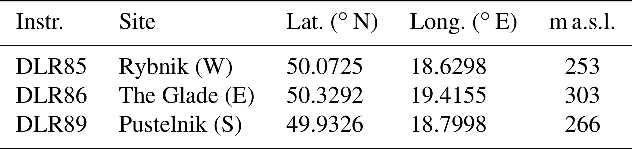
The measurement sites differ to some extent in the surrounding land surface and vegetation. DLR85 is deployed in the west of the USCB next to a private airfield mostly used for parachuting activities and flight training schools. The land surface towards the south-westerly direction is flat. However, the airfield is close to a forest located to the north-west of the wind lidar. DLR86 is placed in the east of the USCB, 62 km from DLR85. The area is surrounded by forest. The southern instrument DLR89 is deployed in the vicinity of the barrier lake Goczałkowickie. The linear distance between the instrument and the bank is roughly 500 m.
The Doppler wind lidars were programmed to perform velocity azimuth display (VAD) scans continuously. To retrieve vertical profiles of not only wind but also turbulence, the VAD scans were performed with two different elevation angles. A series of 24 VAD scans with an elevation angle of 75∘ are followed by six scans with an elevation angle of 35.3∘. The 75∘ scans were chosen to allow retrievals of mean wind speed and direction profiles with a small cone angle, covering at least the whole boundary layer. Filtered sine-wave fitting (FSWF) according to Smalikho (2003) was used to calculate wind speed and wind direction from line-of-sight velocities. While the 75∘ scans are also used to retrieve turbulence kinetic energy dissipation rate, an elevation angle of 35.3∘ is necessary to derive turbulent kinetic energy, integral length scale, and momentum fluxes according to Smalikho and Banakh (2017). As described in Stephan et al. (2018b), boundary layer height can be estimated through detection of the height at which the eddy dissipation rate (EDR) drops below a value of 10−4 m2 s−3. As an example, Fig. 3 depicts EDR and PBL height as retrieved from 75∘ scans of the three wind lidars on 06 June 2018. The uncertainty of wind speed retrievals with the FSWF method depends on the signal-to-noise ratio of line-of-sight velocity measurements (Stephan et al., 2018a). We consider an uncertainty of 0.2 m s−1, which is particularly critical under low wind conditions.
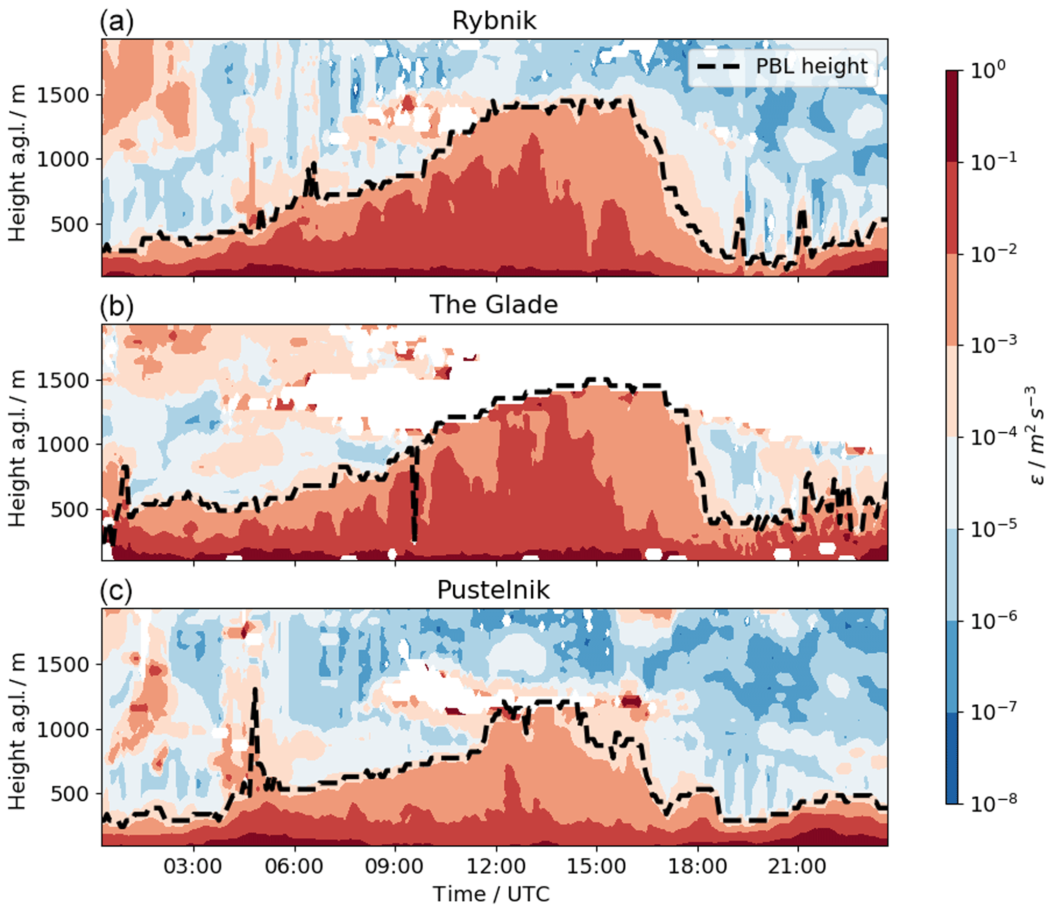
Figure 3Wind lidar profiles of eddy dissipation rate (EDR) on 6 June at the three locations Rybnik/DLR85 (a), the Glade/DLR86 (b), and Pustelnik/DLR89 (c). We performed mobile FTS transects on this day in the morning from 07:00 to 08:00 and around noon (09:30 to 10:30). Dashed lines represent the respective PBL heights. EDR greater than 10−4 m2 s−3 corresponds to PBL values. Note, that the PBL height at the station Pustelnik/DLR89 is shallower compared to the other two stations. This is generally observed throughout the measurement campaign.
2.3 Cross-sectional flux method
The cross-sectional flux method as discussed by Varon et al. (2018) is an established tool typically used for airborne in situ observations (White et al., 1976; Mays et al., 2009; Cambaliza et al., 2014, 2015; Conley et al., 2016). It has also been applied to airborne CH4 (partial) column measurements (Krings et al., 2011, 2013; Tratt et al., 2011, 2014; Amediek et al., 2017). Based on the mass balance assumption, the strength Q of a CH4 point source such as a coal mine ventilation shaft can be calculated by integrating the product of CH4 concentration enhancements and wind speed along a plume cross section. Approximating the integral by a sum over all cross-plume measurements i, the source strength Q in kilograms per second is given by
where we assume the horizontal coordinates xi and yi along and across plume direction. ΔXCH4 (ppm) is translated into the plume enhancement ΔΩ (kg m−2) by
with the molar mass and the Avogadro constant Na. Ueff(xi, yi) is an effective wind speed representative of plume dispersion. The distance Δyi is the cross-plume segment for which the ΔΩ(xi, yi) enhancement is assumed to be representative. We choose the measurements i to be individual stops of the stop-and-go patterns; i.e. we average quantities over individual stops. For estimating wind speed and wind direction, we choose the distance-weighted average of all three wind lidar profiles interpolated to the time of observation, as the baseline wind scenario. The vertical profiles of wind speed (wind direction) are then averaged over the PBL to represent Ueff (yi) in Eq. (2).
There are several caveats and sources of error to this method. (1) The measurement vehicle has to follow public roads, which are not always perpendicular to the plume direction. Therefore, we calculate the cross-plume segment Δyi by
where dsi is the driven distance between two stops of the stop-and-go pattern and αi is the relative angle between the PBL-averaged wind direction and the driving direction. (2) The calculation of ΔXCH4 requires a well-defined XCH4 background removal, which translates into the operational requirement to sample background air on both sides of the plume. (3) We assume that the wind direction remains constant over the sampling duration, which typically is 1 to 1.5 h. (4) The effective wind speed Ueff must be accurate and representative for the observed plume enhancement ΔXCH4. Relative errors in effective wind speed or its representativeness equal relative errors in estimated emissions, which is particularly striking under low wind speed conditions. We discuss these caveats along with the data and errors in Sects. 3 and 4.
Figure 4 displays five transects: one morning and one noon transect on 24 May, one transect on 1 June, and again one morning and one noon transect on 6 June covering different mines and shafts in the USCB. The panels on the left illustrate the locations of observations relative to the nearest mining ventilation shafts. The wind speed and direction are indicated as small wind barbs. Note that for 1 June the wind speed was below 5 kn (i.e. always below 2.5 m s−1) and therefore wind barbs are not displayed. However, wind direction measured by the wind lidars reveals a general south-easterly wind direction. Right-hand side panels show the timeline of all measurements of the EM27/SUN as grey dots together with their respective local stop-wise averages as black crosses. The background XCH4 concentration (dashed black lines in Fig. 4) is based on a linear least-squares (in time) fit of the measurements before and after the plume transect. For our analysis, we selected all cases for which (1) we measured a clear background signal before and after crossing the plume, (2) the wind direction was roughly constant as indicated by the wind lidars, and (3) the overall transect duration does not exceed 1.5 h. All transects and their best-estimate emissions calculated with the baseline wind scenario are described in detail in this section and summarized in Table 2. Discussion of errors follows in Sect. 4.
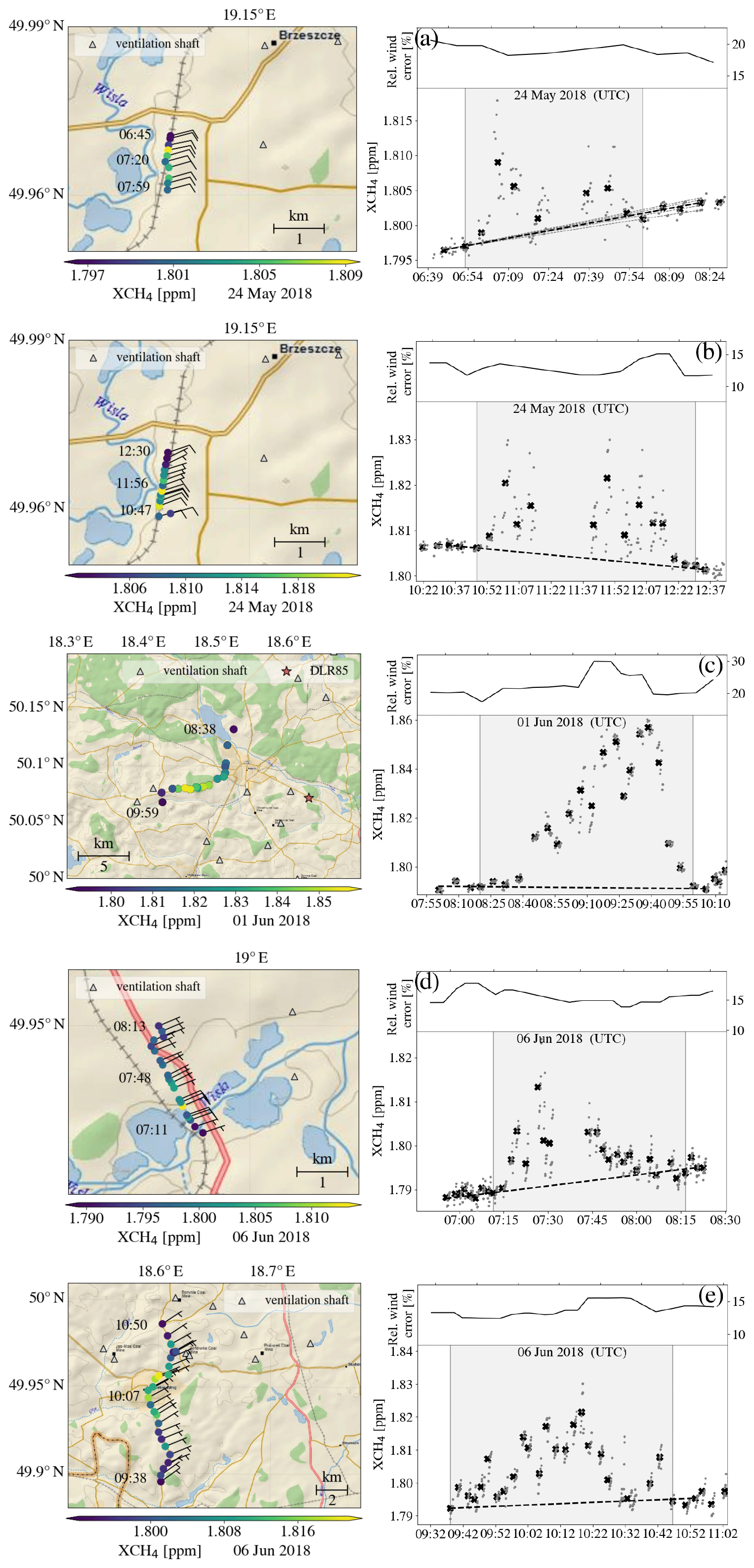
Figure 4XCH4 measured for five transects downwind of the coal mine ventilation in the USCB (panel rows a–e). Left panels display the driven path and the locations of each observation. Wind barbs indicate the wind direction. Note that on 1 June wind speed was very low (<2.5 m s−1) and the wind barbs are not resolved. However, the general wind direction was south-east. The targeted mining ventilation shafts are marked as grey triangles. Right-hand panels display measured XCH4 as grey dots and respective local stop-wise averages as black crosses. The best-estimate background XCH4 is indicated as a dashed black line. Grey areas represent the measurements identified as intra-plume. The black line on top of every right-hand side panel displays the combined relative wind error for each measurement. Dashed grey lines in panel (a) illustrate all background options contributing to the background related error. Geographic maps from ESRI (2019).
On 24 May in the morning (panel row a in Fig. 4), we drove in stop-and-go patterns with stops roughly every 100 m about 2 km west of a ventilation shaft. The target shaft belongs to a mine with four shafts in total. The next closest ventilation shaft was located about 2 km to the north, and no other known shafts were located upwind. Observed plume enhancements ΔXCH4 were up to 15 ppb with a maximum around 07:00. The best-estimate emissions Q are 6±1 kt a−1. Later the same day (panel row b in Fig. 4), we observed the same ventilation shaft but driving from south to north. The transect was interrupted for nearly half an hour due to technical issues from 11:15 to 11:41 UTC; however, we finished the transect afterwards. Maximum ΔXCH4 reached roughly 30 ppb around 11:45. Estimated emissions Q are 10±1 kt a−1, nearly 70 % higher than for the morning transect, which is particularly examined in Sect. 5. Throughout our observations in the morning and around noon, the XCH4 background south of the plume is roughly 4 to 5 ppb higher compared to the north.
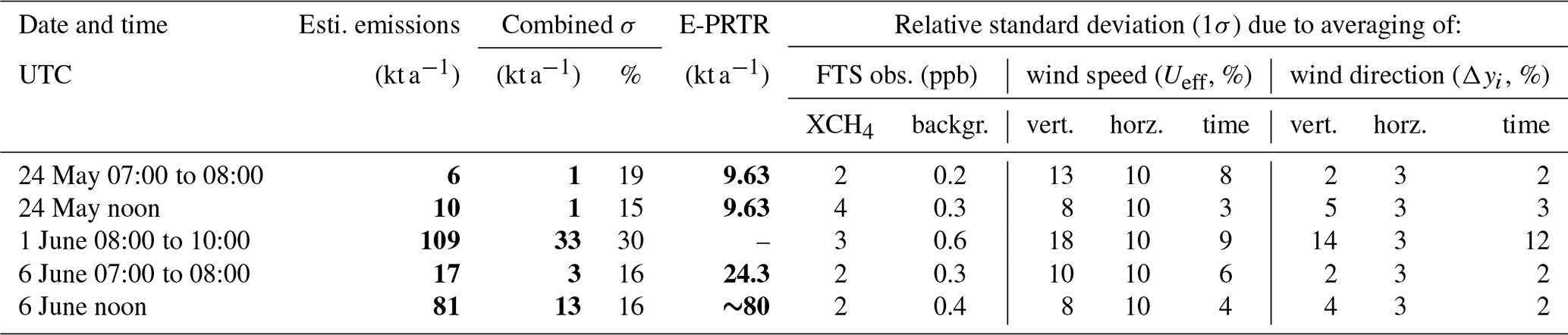
Table 2Overview of successful plume transects along with relative standard deviations of the primary sources of uncertainty. Error estimation procedures are explained in the main text. Bold numbers represent estimated emissions and errors together with the respective E-PRTR 2014 entries in the fifth column, which are the mine-wise reported values distributed evenly to every single listed shaft of each mine. Several upwind sources do not allow accurate source attribution on 1 June, and hence no E-PRTR estimate is reported. E-PRTR CH4 sources contributing to the observations of the noon transect on 6 June amount to roughly 80 kt a−1, if only considering mining ventilation shafts in the near surroundings (20 km radius). However, far upwind (60 km) ventilation shafts can influence the measurements although all mines located in the direct wind direction are listed with 0 kt a−1 and reach 13 kt a−1 somewhat north of the mean wind direction.
On 1 June (panel row c in Fig. 4), we performed a transect at the western border of the USCB (green dots in Fig. 1). The wind lidar data from the nearby DLR85 (11 km distance to the observations) revealed particularly low wind speeds (<2.5 m s−1). Source attribution to individual ventilation shafts is challenging since a group of upwind mining shafts contributes to the measured enhancements. ΔXCH4 values peaked at about 60 ppb around 09:30 UTC at the end of the 1.5 h north-to-south transect. The distance of our observatory to the closest mining shaft was always greater than 4 km. The CH4 emission for the group of shafts is estimated as 109±33 kt a−1.
Clear-sky conditions on the 6 June 2018 enabled us to observe two targets on one day, one in the morning and one around noon. In the morning around 07:00 UTC, we started observing a mine with two shafts at the south-east border of the USCB (red dots in Fig. 1). With the wind blowing from east-north-east, we sampled 1 to 2 km west of the shafts (panel row d in Fig. 4). With the CRDS on board, we were able to assess the rough position of the plume as we could see ground-based in situ enhancements online while moving the truck. Once we reached background CH4 levels in the south, we started sampling with the FTS and moved northward with an average step size of 100 m. Maximum enhancements ΔXCH4 reached roughly 35 ppb around 07:30. Estimated emissions Q amount to 17±3 kt a−1. We measured a difference of +4 ppb between southern and northern background values.
For the second transect on 6 June (purple dots in Fig. 1 and panel row e in Fig. 4), the wind was also from the north-easterly direction. We aimed at measuring a cross section through the southern part of the USCB sampling roughly every 500 m moving from south to north. Downwind (by about 1 to 2 km) of a group of four shafts close to our track, we measured XCH4 enhancements exceeding 30 ppb, from which we calculate total emissions Q of 81±13 kt a−1.
The errors reported for the emission estimates in Sect. 3 are composed of several contributions from terms in Eq. (2): the estimated errors for ΔΩ which partition into the measurement error and the error for background removal; the errors associated with effective wind speed Ueff, which partition into errors related to vertical, horizontal, and temporal averaging of the wind lidar measurements; and the errors in Δyi, which are dominated by the errors in the relative angle between wind directions and driving directions.
As a measure for the measurement error attributed to XCH4, we take the standard deviation among all measurements collected during an individual stop of our stop-and-go pattern. These standard deviations exhibit a maximum of 4 ppb for the noon transect on 24 May. Short distances to the mining shaft and wind speeds around 6 m s−1 imply large variability in the CH4 column above the FTS. For the same day in the morning, the relative CH4 standard deviations for a transect at the same shaft were smaller (2 ppb). The actual instrument precision of the FTS XCH4 measurements is on the order of roughly 0.3 ppb (0.02 %). Thus, the error estimate is driven by atmospheric variability.

Figure 5Relative differences between the best-estimate (weighted averaged) wind speed and sensitivity calculations using wind speed from individual wind lidars. Different colours represent different transects. Individual symbols refer to the wind information source used. The panel (b) is a zoom of the panel (a), but it omits data from 1 June.
The error associated with XCH4 background removal is estimated as the standard deviation of all possible combinations of non-plume signals observed before and after crossing the plume during the generally 1 to 1.5 h long transects. We define an observation as intra-plume if the absolute difference between two consecutive measurements is at least 0.5 ppb greater than the average standard deviation of all measurements. We then linearly fit all possible background estimates as illustrated by grey dashed lines in Fig. 4a. The average of all these background options is defined as the best-estimate background. Their standard deviation is considered in the error budget. The best-estimate XCH4 background is then used to obtain the plume enhancements ΔXCH4 by subtracting the background from the measured XCH4. Overall the background removal standard deviation is smaller than 0.6 ppb, which is small compared to other sources of error. For 6 June, we rely on the on-board in situ measurements to locate the start and end points of the plume. We observed the in situ concentrations on the fly and started with the FTS measurements once we observed constantly low CH4 concentrations.
Errors related to the estimate of effective wind speed Ueff typically dominate the error budget. Our baseline wind scenario averages the lidar wind profiles vertically throughout the PBL and considers the errors arising from temporal wind speed variability throughout one plume transect and from distance-weighted averaging between the three wind lidars. We take the standard deviations among all wind speed measurements inside the PBL to quantify the error related to vertical averaging. The respective error estimates range from 8 % to 18 %, with larger errors occurring under low wind speed conditions as observed on 1 June (Ueff<2.5 m s−1). The error due to temporal averaging of wind speed is estimated by the respective standard deviations of wind speed during the averaging period. This error ranges from 3 % to 9 %.
Having the advantage of three wind lidars co-deployed in the USCB, we can also assess Ueff errors related to horizontal variability of wind speeds. To this end, we conducted a sensitivity study that calculates the emissions Q with wind information from each single wind lidar instrument, instead of using a horizontal average that is weighted by the distance between lidar and FTS as in our baseline scenario. Distances between XCH4 observations and wind measurements range between 11 and 72 km. Figure shows the relative differences of calculated wind speeds Ueff for all sensitivity runs with respect to the best-estimate baseline scenario (reported in Sect. 3).
Differences between the wind speeds generally increase the larger the distance between the FTS and the wind lidar locations. Differences range between 1 % and 13 % except for distances exceeding 40 km and for low wind speed conditions such as encountered on 1 June, which implies larger errors. For 1 June with Ueff<2.5 m s−1, relative wind speed differences differ substantially if wind information is taken from measurements more than a few tens of kilometres away. Figure also reveals that using wind information from DLR89 causes emission estimates that are higher than for the other wind information sources. Wind measurements of DLR89 are likely influenced by the nearby lake, especially during the prevailing easterly winds. Low surface roughness and low friction above the lake surface could cause the wind speeds – and therefore the emission estimates – to be higher in lower levels compared to the other sites located close to forests. Since the distance of the FTS to the closest wind lidar never exceeded 33 km and since we used distance-weighted averages of the wind measurements, we estimate the error due to horizontal wind speed averaging as 10 %.
Errors due to wind direction translate into errors of the cross-plume segment Δyi. Similar to the error estimation procedures for wind speed, we estimated wind direction errors due to vertical, temporal, and horizontal averaging. In general, these errors are smaller compared to wind speed errors. Vertical averaging yields a standard deviation of 2 % to 5 % except for the low wind speed day 1 June (14 %). Temporal averaging induces errors ranging between 2 % and 3 % again except for 1 June with 12 %. We estimate the error due to horizontal wind direction averaging as 3 % according to the procedure we used to estimate the horizontal wind speed averaging error.
Generally, we take the above individual error contributions, and we propagate them into the reported emission errors for Q by Gaussian error propagation. The error contributions from estimating the effective wind speed Ueff dominate the error budget. An overview of all wind situations for all transects is given in Fig. 5. Every circle refers to a certain time during the transect and the circle size indicates the total relative Ueff error (calculated through Gaussian error propagation from the individual contributions given in Table 2). Solid circles mark best-estimate wind information. Transparent circles indicate data from our sensitivity study based on individual wind lidars. Mainly easterly winds were observed for the transects reported in this study. Wind speeds varied between 4 and 8 m s−1 for all cases except for 1 June, which was challenging for emission estimation since wind speeds were generally low and variable in the deployment region.
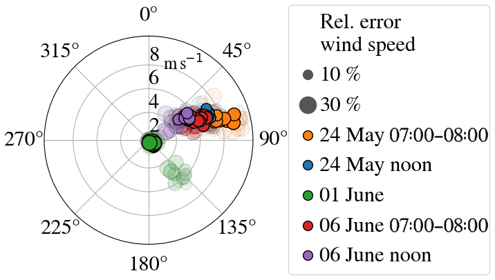
Figure 6The wind rose indicates wind direction and wind speed as occurred during the transects. Different colours mark different days. Size of the circles corresponds to the relative standard deviation in % resulting from averaging wind speed horizontally, within the PBL, and over time. Solid circles mark the best-estimate wind information whereas transparent circles mark wind information that stems from the individual wind lidars directly. During the measurement periods, easterly winds prevailed. Note that for 1 June wind speeds are exceptionally low.
We demonstrate ground-based remote sensing of XCH4 enhancements in the plumes of hard coal mining ventilation shafts several kilometres downwind of the sources. Our observatory truck was equipped with an EM27/SUN FTS measuring direct-sunlight near-infrared absorption spectra. With transect periods of 1 to 1.5 h, the plumes were crossed in stop-and-go patterns. In combination with the data of three co-deployed wind lidars we were able to estimate the emissions for five transects on 3 d.
Our error analysis includes errors related to the FTS measurements and errors related to vertical, horizontal, and temporal averaging of wind speed and wind direction. Combined through Gaussian error propagation these errors range between 15 % and 30 %.
Generally, our best-estimate emissions and the respective errors show broad agreement with the E-PRTR report (European Pollutant Release and Transfer Register, http://prtr.ec.europa.eu/, 2014), which contains emission data reported annually by industrial facilities over Europe including the coal mining branch. This dataset provides annual mean values of CH4 emissions for each mining facility registered. The annual means refer to whole mines, which typically have several shafts to ventilate CH4. We distributed the annual means reported by E-PRTR evenly to all known shafts of every mine. However, our measurements are restricted to a few hours per shaft, and ventilating CH4 of coal mines is a variable process depending on the concentrations in the mine. Furthermore, turbulent processes influence the shape and position of the plume and therefore the measurements. Thus, comparing our snapshot-like measurements with the disaggregated E-PRTR reports can only provide a rough comparison.
Table 2 lists the estimated and reported as well as disaggregated emissions for all five transects. On 24 May, we observed a single shaft in the south-east of the USCB. The reported mine emissions are 9.63 kt a−1. The cross-sectional flux method yields 6±1 kt a−1 for the morning transect and 10±1 kt a−1 for the transect around noon. Background CH4 exhibits a south-to-north gradient, indicating that the measurements could have suffered from CH4 inflow from unknown sources. An observed low-level jet is likely influencing the morning transect. However, differences between single transects are likely as the ventilation system is not emitting constantly. Source attribution becomes challenging measuring downwind of various mines and groups of shafts. Hence, no specific reported emission can be assumed for the transect on 1 June. However, reported emissions likely range between 50 kt a−1 (sum of nearest upwind mines <10 km) and 150 kt a−1 (sum of south-eastern upwind part of the USCB). Our best estimate using the mobile FTS dataset is 109±33 kt a−1. Reported (24.3 kt a−1) and estimated emissions (17±3 kt a−1) generally agree for the morning transect of 6 June. The noon transect on 6 June crossed several possible CH4 sources although the reported emissions are roughly 80 kt a−1. Our best estimate using the mobile FTS data is 81±13 kt a−1, which includes the reported value in the error range. However, many sources are located upwind in the northern part of the USCB within about 60 km distance of the measurements, which also could have influenced the observations but are not included in the sum of the reported emissions for that day.
Enhancing the sampling frequency of the FTS decreased the dwell times significantly (only affects 6 June). This made faster transects possible and helped to avoid changing wind and emission conditions. Faster tracking of the sun would be necessary to allow measuring while driving. Wind information is crucial when using the cross-sectional flux method as relative changes in wind speed equal relative changes in estimated emissions. Particularly low wind speed situations suffer from large discrepancies in the estimates when using wind information from different instruments. Thus, the error budget is dominated by atmospheric variability. Precise wind measurements on board the observational truck would help to reduce the wind-induced errors. CH4 imaging instruments could guide the mobile FTS, providing position and extent of the target plume.
Summarized, our approach enables the emission estimation of CH4 with good confidence (15 % to 30 %). However, the method is restricted to direct sunlight and stable wind conditions. Together with detailed wind information and in situ CH4 measurements, a modified mobile FTS is a flexible, fast (1 to 1.5 h), and accurate (combined relative error of 15 % to 30 %) possibility to estimate coal mine CH4 emissions reliably.
The data are available from the author upon request.
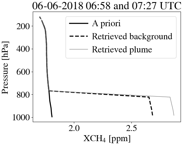
Figure A1A priori versus retrieved CH4 profile. Note, that the retrieval only scales the lower part of the a priori profile up to the expected maximum PBL height of roughly 800 hPa (1700 m a.g.l.). The grey line represents an intra-plume measurement.
AL wrote the paper except for Sect. 2.2, which was written by NW, who also took an active part during the campaign deploying the wind lidars and retrieving and providing wind lidar data. AL, RK, LS, SW, SD, MS, AF, AD, and DD operated the EM27/SUN spectrometer in the field during the campaign and collected and shared the data. RK and JK developed the SunTracker software, which made mobile measurements possible. PJ and ALN supported the selection of the target shafts with CH4 forecasts for the region. TK provided shaft-wise E-PRTR geolocation and emission data retrieved from the E-PRTR dataset (E-PRTR, 2014). AB, FH, MF, JC, and FD supported preparations for the measurement campaign, contributed to the spectral retrievals, and assisted with data post-processing. JN and JS provided detailed information about coal mining and CH4 ventilation and functioned as local advisers. AF coordinated the CoMet campaign operations. AB and AR developed the research question.
The authors declare that they have no conflict of interest.
This article is part of the special issues “CoMet: a mission to improve our understanding and to better quantify the carbon dioxide and methane cycles”. It is not associated with a conference.
We acknowledge funding for the CoMet campaign by BMBF (German Federal Ministry of Education and Research) through AIRSPACE (FKZ (grant no. 01LK1701A)). We thank DLR VO-R for funding the young investigator research group “Greenhouse Gases”. We gratefully acknowledge the constructive comments of two anonymous referees as well as the helpful comments of Mathieu Quatrevalet (DLR-Institute of Atmospheric Physics, Oberpfaffenhofen, Germany) on an earlier version of the manuscript.
The CoMet campaign has been supported by BMBF (German Federal Ministry of Education and Research) through AIRSPACE (FKZ (grant no. 01LK1701A)).
The article processing charges for this
open-access publication were covered by a Research
Centre of the Helmholtz Association.
This paper was edited by Cheng Liu and reviewed by two anonymous referees.
Amediek, A., Ehret, G., Fix, A., Wirth, M., Büdenbender, C., Quatrevalet, M., Kiemle, C., and Gerbig, C.: CHARM-F – a new airborne integrated-path differential-absorption lidar for carbon dioxide and methane observations: measurement performance and quantification of strong point source emissions, Appl. Optics., 56, 5182–5197, https://doi.org/10.1364/AO.56.005182, 2017. a, b
Bousquet, P., Ciais, P., Miller, J., Dlugokencky, E. J., Hauglustaine, D., Prigent, C., Van der Werf, G., Peylin, P., Brunke, E.-G., Carouge, C., Langenfelds, R., Lathière, J., Papa, F., Ramonet, M., Schmidt, M., Steele, L. P., Tyler, S. C., and White, J.: Contribution of anthropogenic and natural sources to atmospheric methane variability, Nature, 443, 439–443, 2006. a, b
Butz, A., Dinger, A. S., Bobrowski, N., Kostinek, J., Fieber, L., Fischerkeller, C., Giuffrida, G. B., Hase, F., Klappenbach, F., Kuhn, J., Lübcke, P., Tirpitz, L., and Tu, Q.: Remote sensing of volcanic CO2, HF, HCl, SO2, and BrO in the downwind plume of Mt. Etna, Atmos. Meas. Tech., 10, 1–14, https://doi.org/10.5194/amt-10-1-2017, 2017., 2017. a, b, c, d, e, f, g
Cambaliza, M. O. L., Shepson, P. B., Caulton, D. R., Stirm, B., Samarov, D., Gurney, K. R., Turnbull, J., Davis, K. J., Possolo, A., Karion, A., Sweeney, C., Moser, B., Hendricks, A., Lauvaux, T., Mays, K., Whetstone, J., Huang, J., Razlivanov, I., Miles, N. L., and Richardson, S. J.: Assessment of uncertainties of an aircraft-based mass balance approach for quantifying urban greenhouse gas emissions, Atmos. Chem. Phys., 14, 9029–9050, https://doi.org/10.5194/acp-14-9029-2014, 2014. a
Cambaliza, O. L. M., Shepson, P., Bogner, J., Caulton, R. D., Stirm, B., Sweeney, C., Montzka, A. S., Gurney, K., Spokas, K., Salmon, O., Lavoie, T., Davis, K., Karion, A., Moser, B., and Richardson, S.: Quantification and source apportionment of the methane emission flux from the city of Indianapolis, Elem. Sci. Anth., 3, 000037, https://doi.org/10.12952/journal.elementa.000037, 2015. a
Chen, J., Viatte, C., Hedelius, J. K., Jones, T., Franklin, J. E., Parker, H., Gottlieb, E. W., Wennberg, P. O., Dubey, M. K., and Wofsy, S. C.: Differential column measurements using compact solar-tracking spectrometers, Atmos. Chem. Phys., 16, 8479–8498, https://doi.org/10.5194/acp-16-8479-2016, 2016. a, b, c
Conley, S., Franco, G., Faloona, I., Blake, D. R., Peischl, J., and Ryerson, T. B.: Methane emissions from the 2015 Aliso Canyon blowout in Los Angeles, CA, Science, 351, 1317–1320, https://doi.org/10.1126/science.aaf2348, 2016. a
E-PRTR 2014: The European Pollutant Release and Transfer Register, available at: http://prtr.ec.europa.eu (last access: 13 August 2018), 2014. a
ESRI: DeLorme World Base Map, available at: http://server.arcgisonline.com/ArcGIS/rest/services/Specialty/DeLorme_World_Base_Map/MapServer/export?bbox=465524.673242,223740.873843,484241.251687,238103.141466&bboxSR=2180&imageSR=2180&size=1500,1151&dpi=96&format=png32&f=imageC, last access: 20 September 2019. a, b
Frey, M., Hase, F., Blumenstock, T., Groß, J., Kiel, M., Mengistu Tsidu, G., Schäfer, K., Sha, M. K., and Orphal, J.: Calibration and instrumental line shape characterization of a set of portable FTIR spectrometers for detecting greenhouse gas emissions, Atmos. Meas. Tech., 8, 3047–3057, https://doi.org/10.5194/amt-8-3047-2015, 2015. a
Frey, M., Sha, M. K., Hase, F., Kiel, M., Blumenstock, T., Harig, R., Surawicz, G., Deutscher, N. M., Shiomi, K., Franklin, J. E., Bösch, H., Chen, J., Grutter, M., Ohyama, H., Sun, Y., Butz, A., Mengistu Tsidu, G., Ene, D., Wunch, D., Cao, Z., Garcia, O., Ramonet, M., Vogel, F., and Orphal, J.: Building the COllaborative Carbon Column Observing Network (COCCON): long-term stability and ensemble performance of the EM27/SUN Fourier transform spectrometer, Atmos. Meas. Tech., 12, 1513–1530, https://doi.org/10.5194/amt-12-1513-2019, 2019. a, b
Gerilowski, K., Tretner, A., Krings, T., Buchwitz, M., Bertagnolio, P. P., Belemezov, F., Erzinger, J., Burrows, J. P., and Bovensmann, H.: MAMAP – a new spectrometer system for column-averaged methane and carbon dioxide observations from aircraft: instrument description and performance analysis, Atmos. Meas. Tech., 4, 215–243, https://doi.org/10.5194/amt-4-215-2011, 2011. a
Gisi, M., Hase, F., Dohe, S., and Blumenstock, T.: Camtracker: a new camera controlled high precision solar tracker system for FTIR-spectrometers, Atmos. Meas. Tech., 4, 47–54, https://doi.org/10.5194/amt-4-47-2011, 2011. a, b
Gisi, M., Hase, F., Dohe, S., Blumenstock, T., Simon, A., and Keens, A.: XCO2-measurements with a tabletop FTS using solar absorption spectroscopy, Atmos. Meas. Tech., 5, 2969–2980, https://doi.org/10.5194/amt-5-2969-2012, 2012. a, b
Hase, F., Hannigan, J., Coffey, M., Goldman, A., Höpfner, M., Jones, N., Rinsland, C., and Wood, S.: Intercomparison of retrieval codes used for the analysis of high-resolution, ground-based FTIR measurements, J. Quant. Spectrosc. Ra., 87, 25–52, https://doi.org/10.1016/j.jqsrt.2003.12.008, 2004. a
Hase, F., Frey, M., Blumenstock, T., Groß, J., Kiel, M., Kohlhepp, R., Mengistu Tsidu, G., Schäfer, K., Sha, M. K., and Orphal, J.: Application of portable FTIR spectrometers for detecting greenhouse gas emissions of the major city Berlin, Atmos. Meas. Tech., 8, 3059–3068, https://doi.org/10.5194/amt-8-3059-2015, 2015. a
Hase, F., Frey, M., Kiel, M., Blumenstock, T., Harig, R., Keens, A., and Orphal, J.: Addition of a channel for XCO observations to a portable FTIR spectrometer for greenhouse gas measurements, Atmos. Meas. Tech., 9, 2303–2313, https://doi.org/10.5194/amt-9-2303-2016, 2016. a
Helmig, D., Rossabi, S., Hueber, J., Tans, P., Montzka, S. A., Masarie, K., Thoning, K., Plass-Duelmer, C., Claude, A., Carpenter, L., Lewis, A., and Punjabi, S.: Reversal of global atmospheric ethane and propane trends largely due to US oil and natural gas production, Nat. Geosci., 9, 490–495, https://doi.org/10.1038/ngeo2721, 2016. a
IPCC: Climate Change 2013: The Physical Science Basis. Contribution of Working Group I to the Fifth Assessment Report of the Intergovernmental Panel on Climate Change, Cambridge University Press, Cambridge, United Kingdom and New York, NY, USA, https://doi.org/10.1017/CBO9781107415324, 2013. a
Jöckel, P., Tost, H., Pozzer, A., Kunze, M., Kirner, O., Brenninkmeijer, C. A. M., Brinkop, S., Cai, D. S., Dyroff, C., Eckstein, J., Frank, F., Garny, H., Gottschaldt, K.-D., Graf, P., Grewe, V., Kerkweg, A., Kern, B., Matthes, S., Mertens, M., Meul, S., Neumaier, M., Nützel, M., Oberländer-Hayn, S., Ruhnke, R., Runde, T., Sander, R., Scharffe, D., and Zahn, A.: Earth System Chemistry integrated Modelling (ESCiMo) with the Modular Earth Submodel System (MESSy) version 2.51, Geosci. Model Dev., 9, 1153–1200, https://doi.org/10.5194/gmd-9-1153-2016, 2016. a
Kille, N., Chiu, R., Frey, M., Hase, F., Sha, M. K., Blumenstock, T., Hannigan, J. W., Orphal, J., Bon, D., and Volkamer, R.: Separation of Methane Emissions From Agricultural and Natural Gas Sources in the Colorado Front Range, Geophys. Res. Lett., 46, 3990–3998, https://doi.org/10.1029/2019GL082132, 2019. a
Kirschke, S., Bousquet, P., Ciais, P., Saunois, M., Canadell, J. G., Dlugokencky, E. J., Bergamaschi, P., Bergmann, D., Blake, D. R., Bruhwiler, L., Cameron-Smith, P., Castaldi, S., Chevallier, F., Feng, L., Fraser, A., Heimann, M., Hodson, E. L., Houweling, S., Josse, B., Fraser, P. J., Krummel, P. B., Lamarque, J.-F., Langenfelds, R. L., Le Quéré, C., Naik, V., O'Doherty, S., Palmer, P. I., Pison, I., Plummer, D., Poulter, B., Prinn, R. G., Rigby, M., Ringeval, B., Santini, M., Schmidt, M., Shindell, D. T., Simpson, I. J., Spahni, R., Steele, L. P., Strode, S. A., Sudo, K., Szopa, S., van der Werf, G. R., Voulgarakis, A., van Weele, M., Weiss, R. F., Williams, J. E., and Zeng, G.: Three decades of global methane sources and sinks, Nat. Geosci., 6, 813–823, https://doi.org/10.1038/ngeo1955, 2013. a
Klappenbach, F., Bertleff, M., Kostinek, J., Hase, F., Blumenstock, T., Agusti-Panareda, A., Razinger, M., and Butz, A.: Accurate mobile remote sensing of XCO2 and XCH4 latitudinal transects from aboard a research vessel, Atmos. Meas. Tech., 8, 5023–5038, https://doi.org/10.5194/amt-8-5023-2015, 2015. a, b, c
Kostinek, J., Roiger, A., Davis, K. J., Sweeney, C., DiGangi, J. P., Choi, Y., Baier, B., Hase, F., Groß, J., Eckl, M., Klausner, T., and Butz, A.: Adaptation and performance assessment of a quantum and interband cascade laser spectrometer for simultaneous airborne in situ observation of CH4, C2H6, CO2, CO and N2O, Atmos. Meas. Tech., 12, 1767–1783, https://doi.org/10.5194/amt-12-1767-2019, 2019. a
Krings, T., Gerilowski, K., Buchwitz, M., Reuter, M., Tretner, A., Erzinger, J., Heinze, D., Pflüger, U., Burrows, J. P., and Bovensmann, H.: MAMAP – a new spectrometer system for column-averaged methane and carbon dioxide observations from aircraft: retrieval algorithm and first inversions for point source emission rates, Atmos. Meas. Tech., 4, 1735–1758, https://doi.org/10.5194/amt-4-1735-2011, 2011. a
Krings, T., Gerilowski, K., Buchwitz, M., Hartmann, J., Sachs, T., Erzinger, J., Burrows, J. P., and Bovensmann, H.: Quantification of methane emission rates from coal mine ventilation shafts using airborne remote sensing data, Atmos. Meas. Tech., 6, 151–166, https://doi.org/10.5194/amt-6-151-2013, 2013. a
Mays, K. L., Shepson, P. B., Stirm, B. H., Karion, A., Sweeney, C., and Gurney, K. R.: Aircraft-Based Measurements of the Carbon Footprint of Indianapolis, Environ. Sci. Technol., 43, 7816–7823, https://doi.org/10.1021/es901326b, 2009. a
Miller, S. M., Wofsy, S. C., Michalak, A. M., Kort, E. A., Andrews, A. E., Biraud, S. C., Dlugokencky, E. J., Eluszkiewicz, J., Fischer, M. L., Janssens-Maenhout, G., Miller, B. R., Miller, J. B., Montzka, S. A., Nehrkorn, T., and Sweeney, C.: Anthropogenic emissions of methane in the United States, P. Natl. Acad. Sci. USA, 110, 20018–20022, https://doi.org/10.1073/pnas.1314392110, 2013. a
Nisbet, E. G., Dlugokencky, E. J., and Bousquet, P.: Methane on the Rise – Again, Science, 343, 493–495, https://doi.org/10.1126/science.1247828, 2014. a
Nisbet, E. G., Dlugokencky, E. J., Manning, M. R., Lowry, D., Fisher, R. E., France, J. L., Michel, S. E., Miller, J. B., White, J. W. C., Vaughn, B., Bousquet, P., Pyle, J. A., Warwick, N. J., Cain, M., Brownlow, R., Zazzeri, G., Lanoisellé, M., Manning, A. C., Gloor, E., Worthy, D. E. J., Brunke, E.-G., Labuschagne, C., Wolff, E. W., and Ganesan, A. L.: Rising atmospheric methane: 2007–2014 growth and isotopic shift, Global Biogeochem. Cy., 30, 1356–1370, https://doi.org/10.1002/2016GB005406, 2016. a
Rothman, L., Gordon, I., Barbe, A., Benner, D., Bernath, P., Birk, M., Boudon, V., Brown, L., Campargue, A., Champion, J.-P., Chance, K., Coudert, L., Dana, V., Devi, V., Fally, S., Flaud, J.-M., Gamache, R., Goldman, A., Jacquemart, D., Kleiner, I., Lacome, N., Lafferty, W., Mandin, J.-Y., Massie, S., Mikhailenko, S., Miller, C., Moazzen-Ahmadi, N., Naumenko, O., Nikitin, A., Orphal, J., Perevalov, V., Perrin, A., Predoi-Cross, A., Rinsland, C., Rotger, M., Šimecková, M., Smith, M., Sung, K., Tashkun, S., Tennyson, J., Toth, R., Vandaele, A., and Auwera, J. V.: The HITRAN 2008 molecular spectroscopic database, J. Quant. Spectrosc. Ra., 110, 533–572, https://doi.org/10.1016/j.jqsrt.2009.02.013, 2009. a
Schwietzke, S., Sherwood, O. A., Bruhwiler, L. M., Miller, J. B., Etiope, G., Dlugokencky, E. J., Michel, S. E., Arling, V. A., Vaughn, B. H., White, J. W., and Tans, P. P.: Upward revision of global fossil fuel methane emissions based on isotope database, Nature, 538, 88–91, https://doi.org/10.1038/nature19797, 2016. a, b
Smalikho, I. N.: Techniques of Wind Vector Estimation from Data Measured with a Scanning Coherent Doppler Lidar, J. Atmos. Ocean. Tech., 20, 276–291, https://doi.org/10.1175/1520-0426(2003)020<0276:TOWVEF>2.0.CO;2, 2003. a
Smalikho, I. N. and Banakh, V. A.: Measurements of wind turbulence parameters by a conically scanning coherent Doppler lidar in the atmospheric boundary layer, Atmos. Meas. Tech., 10, 4191–4208, https://doi.org/10.5194/amt-10-4191-2017, 2017. a
Stephan, A., Wildmann, N., and Smalikho, I. N.: Effectiveness of the MFAS method for retrieval of height profiles of speed and direction of the wind from measurements by a Windcube 200s lidar, Proceedings Volume 10833, 24th International Symposium on Atmospheric and Ocean Optics: Atmospheric Physics, Tomsk, Russian Federation, 1083353, https://doi.org/10.1117/12.2504450, 2018a. a
Stephan, A., Wildmann, N., and Smalikho, I. N.: Spatiotemporal visualization of wind turbulence from measurements by a Windcube 200s lidar in the atmospheric boundary layer, Proceedings Volume 10833, 24th International Symposium on Atmospheric and Ocean Optics: Atmospheric Physics, Tomsk, Russian Federation, 1083357, https://doi.org/10.1117/12.2504468, 2018b. a
Toja-Silva, F., Chen, J., Hachinger, S., and Hase, F.: CFD simulation of CO2 dispersion from urban thermal power plant: Analysis of turbulent Schmidt number and comparison with Gaussian plume model and measurements, J. Wind Eng. Ind. Aerod., 169, 177–193, https://doi.org/10.1016/j.jweia.2017.07.015, 2017. a
Toon, G. C.: Atmospheric Line List for the 2014 TCCON Data Release, CaltechDATA, https://doi.org/10.14291/tccon.ggg2014.atm.r0/1221656, 2017. a
Tratt, D. M., Young, S. J., Lynch, D. K., Buckland, K. N., Johnson, P. D., Hall, J. L., Westberg, K. R., Polak, M. L., Kasper, B. P., and Qian, J.: Remotely sensed ammonia emission from fumarolic vents associated with a hydrothermally active fault in the Salton Sea Geothermal Field, California, J. Geophys. Res., 116, D21308, https://doi.org/10.1029/2011JD016282, 2011. a
Tratt, D. M., Buckland, K. N., Hall, J. L., Johnson, P. D., Keim, E. R., Leifer, I., Westberg, K., and Young, S. J.: Airborne visualization and quantification of discrete methane sources in the environment, Remote Sens. Environ., 154, 74–88, https://doi.org/10.1016/j.rse.2014.08.011, 2014. a
Varon, D. J., Jacob, D. J., McKeever, J., Jervis, D., Durak, B. O. A., Xia, Y., and Huang, Y.: Quantifying methane point sources from fine-scale satellite observations of atmospheric methane plumes, Atmos. Meas. Tech., 11, 5673–5686, https://doi.org/10.5194/amt-11-5673-2018, 2018. a
Vasiljević, N., Lea, G., Courtney, M., Cariou, J.-P., Mann, J., and Mikkelsen, T.: Long-range WindScanner system, Remote Sens., 8, 896, https://doi.org/10.3390/rs8110896, 2016. a
Viatte, C., Lauvaux, T., Hedelius, J. K., Parker, H., Chen, J., Jones, T., Franklin, J. E., Deng, A. J., Gaudet, B., Verhulst, K., Duren, R., Wunch, D., Roehl, C., Dubey, M. K., Wofsy, S., and Wennberg, P. O.: Methane emissions from dairies in the Los Angeles Basin, Atmos. Chem. Phys., 17, 7509–7528, https://doi.org/10.5194/acp-17-7509-2017, 2017. a
White, W., Anderson, J., Blumenthal, D., Husar, R., Gillani, N., Husar, J., and Wilson, W.: Formation and transport of secondary air pollutants: ozone and aerosols in the St. Louis urban plume, Science, 194, 187–189, https://doi.org/10.1126/science.959846, 1976. a
Wildmann, N., Vasiljevic, N., and Gerz, T.: Wind turbine wake measurements with automatically adjusting scanning trajectories in a multi-Doppler lidar setup, Atmos. Meas. Tech., 11, 3801–3814, https://doi.org/10.5194/amt-11-3801-2018, 2018. a
Worden, J. R., Bloom, A. A., Pandey, S., Jiang, Z., Worden, H. M., Walker, T. W., Houweling, S., and Röckmann, T.: Reduced biomass burning emissions reconcile conflicting estimates of the post-2006 atmospheric methane budget, Nat. Commun., 8, 2227, https://doi.org/10.1038/s41467-017-02246-0, 2017. a