the Creative Commons Attribution 4.0 License.
the Creative Commons Attribution 4.0 License.
 | 21 Oct 2019
Evaluation of MOPITT Version 7 joint TIR–NIR XCO retrievals with TCCON
Jacob K. Hedelius
Tai-Long He
Dylan B. A. Jones
Bianca C. Baier
Rebecca R. Buchholz
Martine De Mazière
Nicholas M. Deutscher
Manvendra K. Dubey
Dietrich G. Feist
David W. T. Griffith
Frank Hase
Laura T. Iraci
Pascal Jeseck
Matthäus Kiel
Rigel Kivi
Cheng Liu
Isamu Morino
Justus Notholt
Young-Suk Oh
Hirofumi Ohyama
David F. Pollard
Markus Rettinger
Sébastien Roche
Coleen M. Roehl
Matthias Schneider
Kei Shiomi
Kimberly Strong
Ralf Sussmann
Colm Sweeney
Osamu Uchino
Voltaire A. Velazco
Wei Wang
Thorsten Warneke
Paul O. Wennberg
Helen M. Worden
Debra Wunch
Observations of carbon monoxide (CO) from the Measurements Of Pollution In The Troposphere (MOPITT) instrument aboard the Terra spacecraft were expected to have an accuracy of 10 % prior to the launch in 1999. Here we evaluate MOPITT Version 7 joint (V7J) thermal-infrared and near-infrared (TIR–NIR) retrieval accuracy and precision and suggest ways to further improve the accuracy of the observations. We take five steps involving filtering or bias corrections to reduce scatter and bias in the data relative to other MOPITT soundings and ground-based measurements. (1) We apply a preliminary filtering scheme in which measurements over snow and ice are removed. (2) We find a systematic pairwise bias among the four MOPITT along-track detectors (pixels) on the order of 3–4 ppb with a small temporal trend, which we remove on a global scale using a temporally trended bias correction. (3) Using a small-region approximation (SRA), a new filtering scheme is developed and applied based on additional quality indicators such as the signal-to-noise ratio (SNR). After applying these new filters, the root-mean-squared error computed using the local median from the SRA over 16 years of global observations decreases from 3.84 to 2.55 ppb. (4) We also use the SRA to find variability in MOPITT retrieval anomalies that relates to retrieval parameters. We apply a bias correction to one parameter from this analysis. (5) After applying the previous bias corrections and filtering, we compare the MOPITT results with the GGG2014 ground-based Total Carbon Column Observing Network (TCCON) observations to obtain an overall global bias correction. These comparisons show that MOPITT V7J is biased high by about 6 %–8 %, which is similar to past studies using independent validation datasets on V6J. When using TCCON spectrometric column retrievals without the standard airmass correction or scaling to aircraft (WMO scale), the ground- and satellite-based observations overall agree to better than 0.5 %. GEOS-Chem data assimilations are used to estimate the influence of filtering and scaling to TCCON on global CO and tend to pull concentrations away from the prior fluxes and closer to the truth. We conclude with suggestions for further improving the MOPITT data products.
- Article
(7343 KB) - Full-text XML
-
Supplement
(7658 KB) - BibTeX
- EndNote


Carbon monoxide (CO) is an important atmospheric trace gas. It is a tracer of pollution and atmospheric transport and plays an important role in the atmospheric hydroxyl (OH) budget. About 2800 Tg CO yr−1 is emitted globally, with about 45 % of the emissions coming from oxidation of volatile organic compounds (VOCs – predominately methane and isoprene), about 25 % from biomass burning, 25 % from fossil-fuel and domestic-fuel burning, and the rest from vegetation, oceans, and geological activity (Seinfeld and Pandis, 2006). It acts as an indirect greenhouse gas (GHG) as both a minor source of CO2 and by affecting OH concentrations, which in turn affects the lifetime of methane. Its 100-year global warming potential per mass is 1.9 (Forster et al., 2007). The ultimate fate for 90 % of CO is oxidation by OH to form carbon dioxide and HO2. CO has an average global lifetime of about 1–3 months, with a shorter lifetime in the tropics and a longer lifetime in the Southern Hemisphere extratropics (Lelieveld et al., 2016). The moderate lifetime of CO makes it a good tracer for both emissions and transport of pollution.
The Measurements Of Pollution In The Troposphere (MOPITT) is a Canadian instrument aboard the Terra Earth-observing satellite, launched in December 1999. Drummond et al. (2010) describe the instrument in more detail, but briefly, it is a gas correlation radiometer with near-infrared (NIR) and thermal-infrared (TIR) channels. The primary MOPITT mission goal is to quantify CO in the Earth's atmosphere. Space-based observations of CO can provide greater spatial coverage than a few surface observations. However, space-based observations that rely on reflected (e.g., NIR) sunlight can be influenced by surface properties, airglow, and clouds and are more strongly affected by aerosol scattering than solar-viewing instruments. For MOPITT the TIR sensitivity depends on the strength of the temperature contrast between the surface and atmosphere, which is variable across the globe. Due to the physical limitations of passive Earth nadir-viewing remote sensing, satellite instruments often have lower information content per observation than ground-based instruments (e.g., Deeter et al., 2015), especially compared to the Total Carbon Column Observing Network (TCCON), which measures atmospheric absorption of the Sun’s radiance. Ground-based spectrometers often have higher spectral resolution and/or coverage as well as temporal resolution at an individual location. These differences between observing systems make intercomparisons useful in checking for and reducing biases.
While MOPITT data are the longest satellite record of total column CO (Deeter et al., 2017), there are several other satellite instruments that measure column CO, and we mention a few of them here. SCIAMACHY (Scanning Imaging Absorption Spectrometer for Atmospheric CHartographY) aboard Envisat (Environmental Satellite) launched in March 2002 was first compared with ground-based observations in 2005 (Sussmann and Buchwitz, 2005) and later compared with the larger TCCON and found to be biased about 10 ppb lower (Hochstaffl et al., 2018). TROPOMI (TROPOspheric Monitoring Instrument) aboard the Sentinel-5 Precursor was launched in October 2017 and was found to be biased 6 ppb higher than TCCON, with the difference depending on location (Borsdorff et al., 2018). GOSAT-2 (Greenhouse gases Observing SATellite-2) was recently launched in October 2018, and TCCON will be used for its validation.
Most intercomparisons with MOPITT have used aircraft data (e.g, Deeter et al., 2014, 2017, 2019). The first systematic validation of MOPITT CO with ground-based column measurements was by Buchholz et al. (2017), who used the Network for the Detection of Atmospheric Composition Change (NDACC) mid-infrared retrievals. There have been some studies to compare observations from MOPITT with data from a few (three to six) TCCON sites (e.g, Mu et al., 2011; Té et al., 2016), but this is the first to use observations from all the sites in an intercomparison with MOPITT. Continual comparisons of MOPITT observations with other systems ensure data quality and can be used to determine areas of improvement. This intercomparison exercise uses the MOPITT Version 7 joint (V7J) product and ground-based NIR observations from the TCCON.
The rest of this paper is summarized as follows: Sect. 2 describes the different instruments, systems, and datasets used in this study. Section 3 describes our effort to derive filters for MOPITT data and to improve the single-sounding accuracy and precision using bias corrections. Section 4 describes the MOPITT and TCCON comparisons, including sensitivity tests and a comparison of averaging kernels and information content. Section 5 describes data assimilation tests where the GEOS-Chem model is used to estimate how filtering and bias correcting MOPITT data affects global fluxes. Finally we conclude in Sect. 6 with a summary of practical considerations in this study along with suggestions on how MOPITT retrievals might be improved in future iterations, and we summarize our work in Sect. 7.
2.1 MOPITT
The MOPITT instrument aboard the Terra satellite launched in December 1999 has been described elsewhere (Drummond et al., 2010). Briefly, it is a gas-filter correlation radiometer with eight optical channels, of which three have been used since August 2001 for CO observations, two in the TIR band (channels no. 5 and no. 7; 4.617±0.055 µm), and one in the NIR band (channel no. 6; 2.334±0.011 µm). Each channel produces an “average” (A) and “difference” (D) radiance measurement. A linear detector array in each channel allows MOPITT to make observations at four different sounding locations simultaneously. The ground field of view is approximately 22 km×22 km for each sounding. Retrievals from among these four “footprints” or pixels were previously shown to have a bias compared to ground-based column measurements from the NDACC Infrared Working Group (IRWG) (Buchholz et al., 2017). A moving mirror scans cross track for 29 “stares” in each direction for a swath that is approximately 650 km wide, and one back-and-forth sweep takes approximately 26 s.
Terra is in a daytime-descending (nighttime-ascending) Sun-synchronous orbit at an altitude of about 700 km, with a local Equator crossing time at around 10:30 LT (22:30 nighttime) and an inclination angle of 98.4∘. Terra makes 14–15 orbits daily, with an exact repeat time of 16 d. However, with its wide swath width, MOPITT is able to achieve near-global coverage every 3–4 d. The redundancies built into the MOPITT mission allowed for continued measurements after a cooler failure in May 2001 eliminated one of the two optical boards and the usefulness of channels 1–4, leaving channels 5–8 (Drummond et al., 2010). The impact of other early anomalies is minor. No abrupt changes since 2001 are expected to impact the retrievals, with the possible exception of annual hot calibrations, the latest of which being in March 2019 and a separate temporary cooler malfunction in July 2009. Due to the different instrument configuration from the early record, we only include MOPITT data from 2002 to 2017 (inclusive) in this study.
There are different retrieval products corresponding to TIR-only (T) retrievals, NIR-only (N) retrievals, and TIR–NIR (J – joint) retrievals. We chose to make comparisons with the level 2 Version 7 joint (L2, V7J) product because it should theoretically contain the most information. Deeter et al. (2014) noted that the V6 TIR–NIR product has the greatest vertical resolution but has large retrieval errors and bias drift. The TIR-only product has the highest stability, and the NIR only is best at total column CO retrievals. The MOPITT retrievals are performed on a logarithmic scale due to the large variability in CO in the atmosphere (∼ 1 order of magnitude). The state vector includes up to 10 vertical layers of log 10(VMRCO) (dry volume-mixing ratios), surface temperature, and surface emissivity. Retrievals are performed on a grid of 100 hPa spaced layers up to 100 hPa (e.g., surface–900, 900–800 hPa; Deeter, 2017). The top layer retrieved is 100–50 hPa, and above that the prior VMRCO from the model is used due to low sensitivity. The 50–0 hPa layer represents 1.2±0.4% (1σ) of the a priori CO column (1.3 % in SH and 1.0 % in NH). Fractions of CO in this layer compared to the total column are shown in Fig. S1 in the Supplement. The a priori value is from climatological output from the Community Atmosphere Model with Chemistry (CAM-chem; Lamarque et al., 2012) and is described by Deeter et al. (2014). The a priori covariance matrix is described by Deeter et al. (2010). A total column is obtained by a weighted average of the layers, and this can be converted to a column-average dry-air mole fraction (denoted XCO) by dividing by the model total column of dry air included in the MOPITT V7 product that takes into account surface pressure and water content. We focus on only daytime soundings, which are defined as those with a solar zenith angle (SZA) less than 80∘ in the retrieval. In the V7J data product the 100–0 hPa layer is an average of the 100–50 and 50–0 hPa layers, and we use the 100–0 hPa values for our 100–50 hPa layer but use values that are 48 % of this amount for 50–0 hPa based on recommendations of the MOPITT V5 user's guide.
There are a number of previous studies that have compared MOPITT with different observing systems. Because the algorithm has been improved several times since the start of the mission, here we only list validation studies on Versions 6 (released in 2013) and 7 (released in 2016 and used in this study). Recently Version 8 was released (December 2018). Versions prior to 6 are no longer available (https://www2.acom.ucar.edu/mopitt/products, last access: 2 August 2018). Deeter et al. (2014) noticed a bias between the MOPITT V6J column retrievals and aircraft observations of +4.3 ppb (assuming an average total air column density of 2.1×1025 molec. cm−2, roughly 5 % for a global 80 ppb average). They noted a correlation of r=0.89 between the systems and a drift of only 0.15±0.1 ppb yr−1 ( %). The V6J retrievals had an overall positive bias at the surface and 800 hPa layers, a negative bias at the 600 and 400 hPa layers, and a positive bias again at the 200 hPa layer. The bias, drift, and correlation all depended on which data products were compared. Later, the V6J profiles were compared with aircraft measurements over the Amazon Basin (Deeter et al., 2016). Limited maximum aircraft altitudes precluded column retrieval comparisons, but Deeter et al. (2016) noted maximum biases at the 800 hPa of −27 %.
Three studies compared ground-based remote-sensing observations with those from MOPITT (Rakitin et al., 2015; Té et al., 2016; Buchholz et al., 2017). Rakitin et al. (2015) made comparisons between MOPITT V6J L3 and various ground-based remote-sensing sites in Eurasia. There is significant variability in the unadjusted comparisons for different sites in their study, which could be from the influence of averaging kernels (Rodgers and Connor, 2003), but in general MOPITT observations were larger than ground-based observations. Té et al. (2016) compared MOPITT V6J and IASI (Infrared Atmospheric Sounding Interferometer) satellite observations with ground-based observations in an urban site (Paris), a high-altitude site (Jungfraujoch), and a Southern Hemisphere site (Wollongong). They noted good agreement between space and ground-based observations with slopes of 0.91–0.99, with satellite observations being slightly lower. Recently, Buchholz et al. (2017) compared MOPITT V6 observations with those from 14 different ground-based NDACC sites between 78∘ S and 80∘ N and used data from August 2001 to February 2012 for comparisons with V6T, V6N, and V6J. We focus on their V6J comparison results. They found MOPITT to be generally biased high relative to the NDACC, and 11 sites have a bias less than 10 % over land. The all-station mean bias is 5.1 %, and the average correlation is . They noted that the surface type (land or water) had little effect on validation statistics. However, they did note that validation results differed among pixels, and pixel 1 has the lowest correlation while pixel 3 has the highest correlation.
Deeter et al. (2017) is the only systematic global validation study of the MOPITT V7 algorithm. They use aircraft measurements from the HIAPER Pole-to-Pole Observations (HIPPO) campaign and National Oceanic and Atmospheric Administration (NOAA) aircraft flask samples primarily over North America for their validation dataset. They describe the improvements included to create the V7 algorithm. They find that the V7J column observations have a smaller bias and larger r (1.4 ppb and 0.93, respectively) than the V6J product (3.8 ppb and 0.89).
While L1 includes radiance bias corrections, there are no empirical bias corrections to the physics-based retrieval in the L2 V7 MOPITT products. There are retrieval anomaly diagnostics included in the L2 product, but users need to define filters to use for their particular application. For L3, V7J daytime observations where both the signal-to-noise ratio (SNR) of channel no. 5A <1000 and the SNR of channel no. 6A <400 are excluded (Deeter, 2017). All observations from pixel 3 are also excluded due to excessive and unstable noise from NIR measurements from that pixel (Deeter et al., 2015). In this study suggested filters are developed along with a bias correction.
2.2 TCCON
The TCCON is a global network of independently operated solar-viewing Fourier-transform spectrometers (SV-FTS) operated under a common set of standards. From measurements taken by these spectrometers, retrieved estimates of XCO are made (Wunch et al., 2011a, 2015). Because profiles are not a part of the TCCON data product, we focus on validating the MOPITT total columns rather than profiles. Data are quality screened by both individual site operators as well as a centralized team. From sensitivity tests perturbing the algorithm to each known source of uncertainty (e.g., a priori values of VMRs and temperature and surface pressure), GGG2014 XCO systematic errors for TCCON are below 4 % (Wunch et al., 2015). The uncertainty in the scaling slope is 6 % (2σ).
One of the primary uses of the TCCON data has been satellite validation (e.g., Inoue et al., 2016; Kulawik et al., 2016; Wunch et al., 2017b). There are several reasons why TCCON data are considered more accurate than satellite observations and hence a good validation source. (1) Observations are directly pointed at the Sun, which increases the SNR, is insensitive to effects of surface properties, and is insensitive to the effects of both airglow and aerosol scattering (e.g., Zhang et al., 2015). (2) Instruments are operated at a resolution of at least 0.02 cm−1, which provides more information for spectral fitting than most satellite measurements. (3) The network was established in 2004 with contributions from many different institutions. This international collaboration has led to many discoveries on how to reduce errors in Xgas retrievals (e.g., Kiel et al., 2016).
Despite these advantages, there are known sources of uncertainty that could bias the measurements. For example, to tie this to the World Meteorological Organization (WMO) in situ scale, there is a 7 % scaling factor in GGG2014 for XCO (Wunch et al., 2015). This factor is considered large compared to the current uncertainty in spectroscopy, and there is an ongoing effort to determine if this factor is appropriate. In this study we use both the official TCCON XCO product as well as a derived product without the empirical scaling factor applied. For a discussion and current comparison of unscaled TCCON data to the WMO scale, see Sect. S2 in the Supplement.
We compare MOPITT with TCCON from mid-2004 to 2017 (inclusive). Prior to 2007 there were only four TCCON sites (Table 1). During 2007 and 2008 the TCCON grew to nine sites. Table 1 also lists the site locations and number of coincidence days after MOPITT data are filtered.
Iraci et al. (2016a)Goo et al. (2014)Feist et al. (2014)Deutscher et al. (2014)Notholt et al. (2014)Morino et al. (2018)Velazco et al. (2017)Wennberg et al. (2014b)Griffith et al. (2014a)Wunch et al. (2017a)Strong et al. (2017)Dubey et al. (2014b)Lindenmaier et al. (2014)Sussmann and Rettinger (2014)Liu et al. (2018)Iraci et al. (2016b)Blumenstock et al. (2014)Wennberg et al. (2014c, 2016a)Hase et al. (2014)Wennberg et al. (2016b)Sherlock et al. (2014a, b)Pollard et al. (2017)Dubey et al. (2014a)Notholt et al. (2017)Warneke et al. (2014)Té et al. (2014)Wennberg et al. (2014a)De Mazière et al. (2014)Morino et al. (2014b)Kawakami et al. (2014)Kivi et al. (2017)Kivi and Heikkinen (2016)Morino et al. (2014a)Griffith et al. (2014b)Sussmann and Rettinger (2018)Table 1Details for TCCON sites used in this study. Occasionally one site had more than one instrument, as indicated by multiple two-letter IDs.
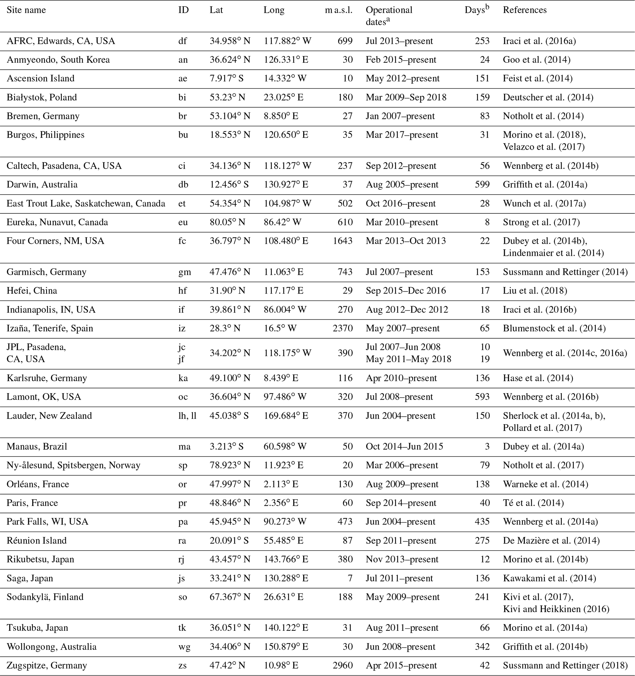
a Operational dates refer to time range where public GGG2014 retrievals are available. b Coincidence days only and after filtering MOPITT data.
2.3 AirCore
AirCore measurements are a novel way to vertically sample the atmosphere to obtain profiles of various gases and have been described elsewhere (Karion et al., 2010; Membrive et al., 2017). Briefly, a coiled tube on the order of 100–300 m long, with an inner diameter on the order of 2–5 mm, is taken to altitude. One end of the tube is sealed, so during ascent it is evacuated and on descent the tube slowly fills with ambient air. Because diffusion is slow over the length of the tube but fast across the 2–5 mm diameter of the tube, air from different altitudes does not mix significantly. Upon landing the vertical profile of the gas is preserved along the length of the tube, with high altitudes near the closed end and low altitudes near the open end. On the ground, the AirCore is analyzed within a few hours, which minimizes molecular diffusion. By pulling the air through and measuring concentrations with a calibrated trace-gas analyzer, a vertical profile can be obtained. AirCore CO is still a developmental product with a sample measurement precision typically less than 5 ppb (Engel et al., 2017). However, stratospheric AirCore CO profile comparisons have shown differences as large as 20 ppb, which could be a result of diffusion in stratospheric AirCore samples, AirCore surface effects, or incorrect AirCore sample end-member assumptions. Accuracy is dependent on the quality of calibration and standards (see Sect. S2).
Often AirCores are flown on balloons that can reach a ceiling of around 30 km (∼10 hPa), depending on the type of balloon. Once altitude is reached, the payload is cut away from the balloon. Higher-altitude data (during rapid descent) often need to be discarded; hence 22 km (∼40 hPa) is the median highest altitude in this dataset. The vertical resolution depends on AirCore tubing dimensions, measurement altitude, recovery time, and temperature but is on the order of 200–1000 m. From 2012 to 2017 there are 36 AirCore profiles available. AirCore profiles are used among other profile measurements to tie TCCON retrievals to the WMO scale (Wunch et al., 2015). Here we use them for sensitivity tests when an approximation of the true atmospheric profile is needed.
Typically a retrieved state vector (e.g., an atmospheric profile) is described as a linearization about the a priori state vector xa (Rodgers, 2000), i.e.,
In this equation, A is the averaging kernel, a matrix in this case, with elements , and x is the true state vector. The term ϵx is a catch-all for any remaining systematic or random uncertainties from instrument calibration or the retrieval. This term is a function of forward-model parameters not perfectly known (b), such as pressure, temperature, pointing, spectroscopy, and modeling of instrument response (e.g., the instrument line shape). c contains other values in the retrieval not used in the forward model, such as convergence criteria. Changes in may thus be related to changes in b and c. Biases in b and c may be approximated as having a linear effect on (Rodgers, 1990). However, these effects may not be accounted for in models, so measurement teams may reduce the effects of these spurious variations by filtering data empirically.
For example, empirical corrections are employed for various gases in the final TCCON products after the physics-based retrievals to improve accuracy up to about 0.1 %, which would otherwise be currently limited to accuracies of about of 2 %–3 % due to spectroscopic uncertainties, especially in O2 (Wunch et al., 2011b, 2015). As a second example, empirical corrections to CO2 measurements from the Orbiting Carbon Observatory-2 (OCO-2) satellite (launched in 2014) did not always improve data at all scales but did reveal areas where the algorithm could be improved (O'Dell et al., 2018; Kiel et al., 2019). Though their studies were for CO2, we apply many of the same methods for CO, including similar truth proxies.
By comparing retrieved data with a truth proxy, some data may stand out as being possibly biased due to the ϵx(b,c) term. These may be filtered out, deweighted, or bias corrected to improve the final product. It is challenging to define a truth proxy because if the true state of the atmosphere were known a priori, the measurement would not be needed in the first place. Rather than using proxies that work for each measurement, we aggregate many measurements to empirically identify artifacts and outliers. We use TCCON and a small-region approximation (SRA – also known as small-area approximation or variation in other studies) as truth proxies. For the SRA we assume that over a sufficiently small region (e.g., ) that is far from point sources the atmosphere is approximately homogeneous and outliers are due to inadequacies in the retrieval.
Filter selection and biases are interdependent; thus our quality-control (QC) and bias-correction process was iterative.
3.1 Pixel-to-pixel bias
Buchholz et al. (2017) observed biases among the four MOPITT pixels. This bias significantly affects our SRA (Sect. 3.2), as a biased value may be chosen as the median. We spatially grid the data in bins and average for each pixel separately over monthly timescales to evaluate variability in the bias. Here and throughout, data are averaged as described in Appendix A. We analyze multiple months but here show results from April and November 2016 in Fig. 1 for the difference between pixels 2 and 4. We choose these two pixels because the instrumental noise is larger for pixel 3 (Deeter et al., 2015) and pixel 1 has a known large global bias (Buchholz et al., 2017), and we would therefore expect the difference between pixels 2 and 4 to be a lower bound on pixel-to-pixel bias. We see large pixel-to-pixel bias polewards of 60∘. Comparing with scenes flagged as snowy or icy by retrievals from MODIS (Moderate Resolution Imaging Spectroradiometer; also aboard Terra), we see that there is some correlation between the bias with the snow or ice scenes. This bias can be positive or negative. For example, we see that pixel 2 is lower than pixel 4 towards the North Pole and is biased positively over land in Antarctica. Over sea ice around Antarctica, pixel 2 is lower than pixel 4. We also compare pixels 1 and 3 to the weighted mean and find that pixel 3 is biased low over land snow or ice and pixel 1 is biased high over both land and water snow or ice. These biases likely arise from the effects snow or ice have on the thermal contrast of the surface and hence affect the TIR channels. For the rest of our analysis, we filter for daytime scenes and remove soundings where the MODIS diagnostics indicate the presence of any snow or ice.

Figure 1On the left (a, b) are average differences in XCO between pixels 2 and 4. On the right (c, d) is the corresponding MODIS snow or ice flag, where 0 indicates all snow or ice and 1 indicates that the scenes were clear of snow or ice. Some correlation is observed between bins with a large pixel-to-pixel bias and snow or ice cover. Here and throughout we use an Eckert IV equal-area projection.
We examine temporal trends in MOPITT pixel bias compared to the weighted mean from all pixels (Fig. 2). Data are averaged globally for each pixel and surface type separately for 15 d bins. This analysis relies on the assumption that on average each pixel samples the same area. We see that the absolute bias of pixel 1 is largest. However, in contrast with Buchholz et al. (2017), we observe a negative rather than positive bias between pixel 1 and the mean in the TIR–NIR retrievals, which may be because their study was of V6 data. Pixel 3 has a smaller absolute bias that is positive. In 2002, the spread of the biases is larger than in 2017. On average, the land and water biases are similar (within 0.4 ppb); however, there is a larger seasonal cycle (∼1.5 ppb) in the bias for the land that may be an artifact of the sampling and averaging global 15 d bins.
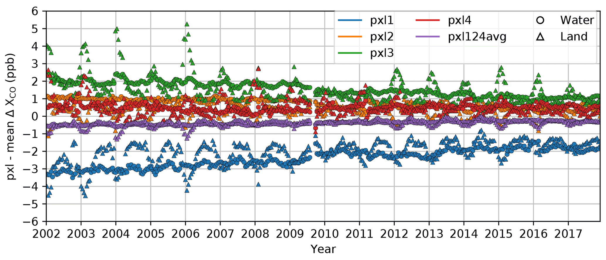
Figure 2Pixel (pxl) biases compared to the weighted mean with time. Data are averaged into 15 d bins separated for land and water soundings. The mean of pixels 1, 2, and 4 is also shown because pixel-3 data are not included in the L3 product. The small gap in 2009 is from a temporary cooler malfunction on 28 July.
One consideration for bias corrections is whether accounting for differences in averaging kernels can account for the bias. Buchholz et al. (2017) noticed a large absolute bias for pixel 1 compared with NDACC observations even after accounting for averaging kernels. To examine the effects of averaging kernels, we find MOPITT soundings within an ellipse ( latitude, longitude) around the center location of AirCore flights on the same day. There are 20 flights with coincident observations and 1933 total corresponding MOPITT soundings. We apply averaging kernels to create simulated MOPITT column retrievals from AirCore profile measurements:
where is the simulated XCO, and ca is the a priori column XCO. x is the dry VMR profile (from AirCore) and should not be confused with the state vector, which is log 10(VMR) for MOPITT. For this study we have defined the MOPITT column-averaging kernel for a pressure level i to be (Appendix B)
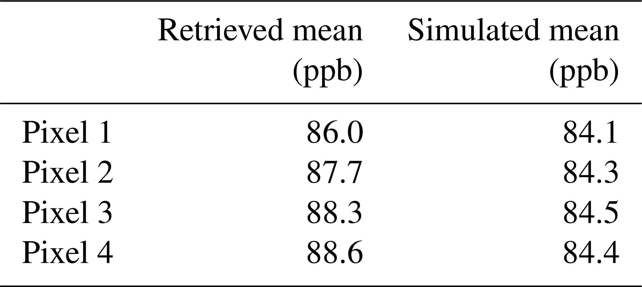
The pressure weighting function h has been described by Connor et al. (2008) and Wunch et al. (2010). We find that the maximum bias for the retrieved columns is between pixels 1 and 4 and is about 8 times larger for the retrieved (2.6 ppb) than for the simulated columns (0.3 ppb; Table 2). For these soundings MOPITT is also biased high compared to the AirCore simulated columns by 3.3 ppb, which is greater than the bias of 0.5–1.4 ppb compared to other aircraft profiles (Deeter et al., 2017).
Table 2Mean values of MOPITT XCO retrievals, colocated with AirCore measurements and separated by pixel, compared to the simulated XCO from applying MOPITT averaging kernels to AirCore profiles for 22 flights.
We make a preliminary pixel bias correction by adjusting soundings over land and water for each pixel separately based on a linear fit to the overall time series shown in Fig. 2. This fit is later improved after filtering (Sect. 3.4). After this adjustment we noticed some residual bias among the histograms, so we also apply a year-to-year pixel bias correction of up to 0.4 ppb that is the same for water and land.
3.2 Small-region approximation
We perform a SRA on the dataset with the preliminary filter for daytime and snow or ice free scenes and preliminary pixel bias correction. In a SRA, data within a specified area and time frame are assumed to be homogeneous, and variation within that area is assumed to be non-physical. There is always some real variation in the atmosphere; however, statistically, for a large sample size these variations are expected to average out. If the area is too small then there will be too few points for an unbiased median. If the area is too large then true atmospheric variability will be significant. A disadvantage of using this method as a “truth” proxy is that it is insensitive to bias on larger scales related to, for example, latitude and surface albedo (e.g., O'Dell et al., 2018, for OCO-2 and CO2).
We use small regions that are approximately 89 km×133 km (, latitude × longitude, at the Equator). Region size is a trade-off between having sufficient points per region and keeping regions small enough that real variations in XCO are small. The effects of different region sizes are described in Sect. S3. To calculate anomalies, we subtract the median from all the points within that region. If the median point does not have at least a degree of freedom (DOF) for the signal then the entire region is discarded. We also require at least 10 points in each region, which retains about 50 % of the SRA bins.
3.3 Quality control filters
Using the SRA “truth” proxy, we can look for correlations of differences to the local median (i.e., anomalies) with various parameters that are or may be related to the retrieval. Table 3 lists parameters we consider for filtering and bias corrections. We make plots similar to those by Wunch et al. (2011b) and O'Dell et al. (2018) (though their studies were of ) of anomalies versus one of the various parameters to aid in determining filter cutoffs (e.g., Fig. 3). Such plots may reveal empirical relationships with features. Similar plots with additional parameters, including some we decided were inappropriate to use as filters, are available in the Supplement (Sect. S4). Several features can be examined in these plots to decide on where to set the filter limits, including the underlying histograms, systematic biases from zero in the mean including spikes, the spread among pixels – which indicates pixel-to-pixel bias, and the root-mean square (RMS) from the SRA – which includes systematic and random deviations from the truth proxy. We define filters based usually on one of the following criteria: (1) absolute mean bias is greater than 2 ppb, (2) the RMS is greater than 6 ppb, or (3) spread of pixel-to-pixel bias is greater than 5 ppb. These criteria are not strict, and we change thresholds if too few data are in a bin (due to possible sampling bias), if too many data are removed, or if the overall trend in the mean seems like it could be corrected by a bias correction.
Several features are apparent in the SRA diagrams (Figs. 3 and S4–S9) that indicate that data may be less reliable. For example, there is a step change in the bias for soundings over land going from day to night. The RMS is much smaller over snow or ice free scenes (flag of 1). We also note large anomalies for low channel 5A SNR which, in agreement with the L3 product filters, suggest it to be a good parameter to filter on. However, the bias is small for low channel 6A SNR soundings; so unlike the L3 product, we do not use it as a filter criterion. We also find that the sum of the retrieval anomaly diagnostics is a better indicator for suspicious data over land than over water. These particular tests also do not support excluding all pixel-3 soundings, though on average it does have a lower and more variable DOF (Deeter et al., 2015). Maps of where data are filtered are available in Figs. S10 and S11. Using these filters reduces the number of daytime soundings to 3.50×10⁸ (of 5.40×10⁸) and reduces the RMS from 3.84 to 2.55 ppb. By comparison, when we apply the L3 filters it reduces data to 3.27×10⁸ daytime soundings and an RMS of 3.02 ppb.
Table 3Parameters in or related to MOPITT retrievals that we considered for filtering and bias correction. Data are excluded if any of the criteria below are met. Mixed surface-type soundings are also excluded.

a Source: I is included in L2 files, R is ratio within L2 files, D is other derivation from L2 files, and E is external. b Difference from the a priori value. AOD is aerosol optical depth. tr is matrix trace.
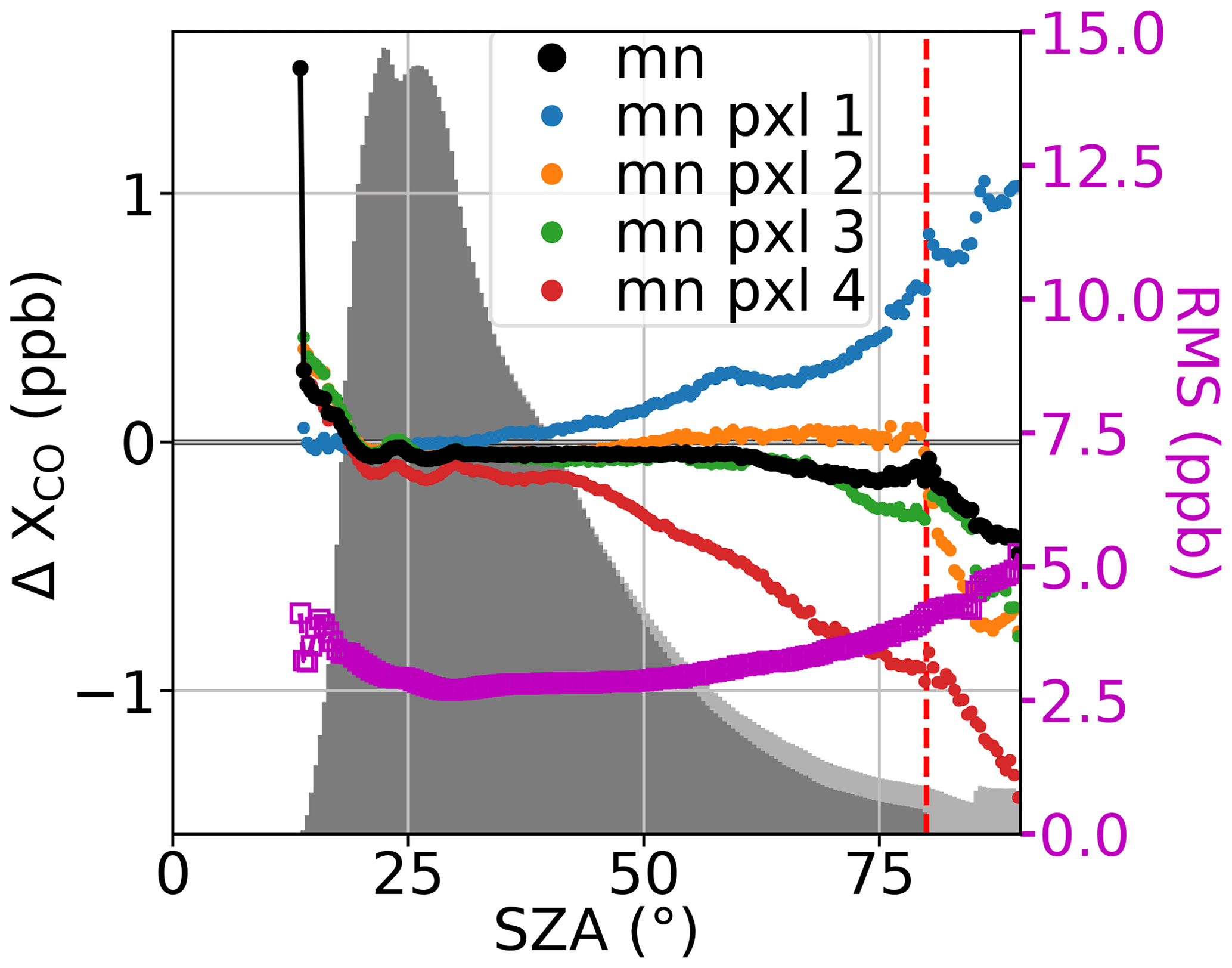
Figure 3Example diagram showing the small-region approximation (SRA) bias as a function of solar zenith angle for water. The black points show the overall mean (mn) bias (minimum 2000 points), the magenta points show the RMS, and the other points show the mean bias for the individual pixels (minimum 300 points). The lighter histogram is of all the data. The darker histogram is data remaining after the SZA and snow or ice filters. Figures like this are used to make filters for and check for bias in MOPITT L2 data. The red line is the filter cutoff at 80∘. The equivalent diagram for land, along with diagrams for other features, is in Sect. S4.
3.4 Bias correction
We observe trends in the mean bias with various parameters (e.g., Figs. 3 and S4–S9). To reduce the likelihood of overfitting, O'Dell et al. (2018) used linear fits as bias corrections only if they removed at least 5 % of the variance for from OCO-2. For XCO from MOPITT, the ratio between the scatter (indicated by RMS) and bias is larger than for from OCO-2; however, over our period of analysis there are about 400 times more data over water and about 100 times more over land. Fitting concerns here primarily relate to how representative the SRA is as a truth proxy and how much the biases would already be accounted for by adjusting individual soundings using averaging kernels.
Even with a criterion of only a 3 % reduction in the overall RMS, the only parameter to meet this is the maximum difference between adjacent levels over land (see Fig. S5j). This feature is larger for strong gradients between levels, which can appear when there are strong surface fluxes or when the retrieval is unstable and oscillates. This instability may be caused by bias related to, for example, spectroscopic errors. Following O'Dell et al. (2018) we make piecewise linear fits to the overall mean over two regimes, split at 100 ppb for a bias correction. The Multivariate Adaptive Regression Splines (MARS) algorithm could also be used to make a piecewise linear fit over a multidimensional dataset. However, it is more likely to overfit the data. When we applied it to the top three most variable fields the RMS for land soundings was not significantly reduced compared with our piecewise fit, so we did not use those results.
In addition to the single “feature” bias correction above, we apply a pixel-to-pixel bias correction after the filtering, described in Sect. 3.3. We perform a second SRA on the filtered data without a pixel bias correction. SRA data are binned separately for each pixel and land or water surface type and averaged over 10 d. On 28 July 2009 one of the coolers on MOPITT malfunctioned, which caused a 2-month instrument shutdown. We separate the period before and after this event and make 16 different linear fits of the bias relative to the all-pixel mean with time (2 for land and water, 4 for pixels, and 2 for time), following the method of York et al. (2004). These linear fits are used to define the pixel-to-pixel bias.
4.1 Coincidence criteria
Various coincidence criteria have been used to match MOPITT soundings with other datasets, such as aircraft measurements, other satellites, or ground-based sensors. For example, Deeter et al. (2014, 2017) used a colocation radius of 50 km for aircraft profiles primarily over North America and a colocation radius of 200 km for aircraft profiles primarily over remote ocean. Over the Amazon, Deeter et al. (2016) also used a colocation radius of 200 km and a colocation time of 24 h. Té et al. (2016) used criteria of latitude and longitude, corresponding to 33 km×33 km over Paris. Buchholz et al. (2017) used a 1∘ radius and ground-based measurements within the same day. Criteria could also include fields such as the temperature of the free troposphere (e.g., around 700 hPa, Wunch et al., 2011b; Nguyen et al., 2014). Sha et al. (2018) used a sampling cone based on the solar azimuth angle at the time of measurement for comparing TCCON with TROPOMI. This is likely unimportant for MOPITT given the larger footprint size (22 km×22 km versus 7 km×7 km). For example, at a 60∘ SZA for a MOPITT pixel centered on a TCCON site at sea level, the TCCON ray would leave the MOPITT pixel at around 11 km or above 250 hPa. For a comparison of SCIAMACHY with NDACC–TCCON, Hochstaffl et al. (2018) found it to be necessary to deweight observations that were further away in time and space from points of comparison. This is likely much less of an issue for this study due to differences in retrieval errors and coincidence scales. For MOPITT the median retrieval error is about 3.5 ppb versus 24.8 ppb for SCIAMACHY. For SCIAMACHY temporal averaging was on the order of a month compared to this study, where we only use TCCON observations within ±30 min. We apply spatial averaging to the MOPITT data typically over areas of (with exceptions noted below). Spatial weighting is not as much of a concern here as for Hochstaffl et al. (2018) with SCIAMACHY because they used coincidence criteria of 500–2000 km radii, which are significantly larger in terms of area (about 8–100 times). However, despite using smaller areas, heterogeneities in CO sources that MOPITT averages over may occasionally introduce bias for real reasons (e.g., Lindenmaier et al., 2014).
We make exceptions to the latitude longitude spatial coincidence criteria for several sites. For sites poleward of 60∘ (eu, sp, and so) we expand the area to because the atmosphere is expected to be well mixed and retrievals are more sparse. For sites in the Los Angeles Basin (ci, jc, and jf), we limit the area to 33.4–34.3∘ N, 116.7–118.8∘ W, because we expect XCO within the basin to be much larger than the surrounding area due to urban emissions. We set the minimum latitude to 34.5∘ N for the AFRC site to avoid the polluted Los Angeles Basin. We average soundings over land and water separately.
Because of the long (13+ year) comparison between MOPITT and TCCON, random representation error is much less important than systematic error. Té et al. (2016) and Buchholz et al. (2017) noted that systematic biases can arise from comparing total column observations (in molec. cm−2) from MOPITT and NDACC when the surface altitudes differ significantly. This effect will be diminished in column averages (XCO) in locations away from strong local surface fluxes; however, different surface altitudes can lead to biases because CO profiles are not completely uniform. Between two TCCON sites only ∼10 km apart in an urban region, Hedelius et al. (2017) noted an difference of nearly 1 ppm. They attributed part of this to the different site altitudes. We estimate the ratio between observations at the surface pressure of TCCON versus the surface pressure of MOPITT soundings. The total column-average dry mole fraction is
The vector x here can be either the retrieved profile or the a priori VMR profile. We use the MOPITT profiles because they are likely more representative of the true atmosphere than TCCON a priori profiles and apply Eq. (4) to find the retrieved and prior MOPITT XCO at the MOPITT sounding surface pressure. We then recalculate h based on the daily average TCCON site surface pressure. When TCCON altitude is lower, the MOPITT surface level is uniformly extended. For higher-altitude sites, the lowest-altitude MOPITT levels are either unused (hj=0) or deweighted. We then calculate XCO based on TCCON surface pressure. Figure 4 shows the ratios between the MOPITT retrieved XCO using the TCCON surface pressure compared to the MOPITT sounding surface pressure for areas. Larger areas are used to get a larger variety in surface pressures. We see that for the high-altitude Zugspitze site, this scaling is particularly large (around 15 %). Over these areas the overall scaling for all sites is 0.996±0.023 (1σ). A scaling factor less than unity is usually due to larger CO mixing ratios near the surface than the rest of the column and lower TCCON site pressure (Hedelius et al., 2017). In this intercomparison, we implicitly account for differences in surface pressure using the h vector. This can make a difference for individual sites by as much as ppb (1σ) (for Zugspitze). However, we have found in practice that accounting for differences in surface pressure makes little difference here on the overall comparison (compare Fig. S12c and f). In aggregate the difference is only ppb (1σ).

Figure 4Scaling factors for MOPITT retrieved profiles if the surface were at the surface of the TCCON site (listed in m a.s.l. in parenthesis). Ordered by increasing site altitude. Soundings within latitude and longitude of TCCON site are used. The center 99 % of data are shown. Blue filled sections indicate data density, similar to a violin plot but using histograms rather than a kernel density estimation due to sufficient data. Black boxes indicate the central 50 % of data, and medians are orange.
4.2 Overall global scaling
MOPITT and TCCON use different a priori VMR profiles and have different averaging kernels (AKs; Sect. 4.4), and these differences in sensitivity need to be taken into account when comparing retrievals from the different instruments. Here we account for differences in AKs and a priori profiles following the methods of Wunch et al. (2011b), which are formally described as method II in Sect. S6.1. Retrievals are also on different vertical grids, and regridding is described in Appendix C. Figure 5 shows the comparison for all sites. We find that MOPITT observations are higher than TCCON by about 6.4 %. This is similar to the 5.1 % positive bias between MOPITT V6J and NDACC total column observations (Buchholz et al., 2017).
We perform a variety of sensitivity tests on the overall global comparison. There are different approaches to account for different a priori VMR profiles and AKs such as the choice of comparison ensemble (Sect. S6). Figure S12 shows the comparison for a variety of tests when AKs are applied differently or not at all. Generally all comparisons show MOPITT to be about 6 %–9 % higher than TCCON, with some exceptions. For method III, where AKs are applied in a manner opposite to method II, the bias is as high as 15 % but is closer to ∼10 % or less. Figure S13 is a series of bar charts of how the different methods compare for each site. We also examine how the scaling changes for different colocation criteria in Figs. S12d and e by halving and doubling the coincidence areas. We find that MOPITT is biased higher than TCCON in these tests by 5 %–7.4 %. Doubling the area decreases R2 for the global comparison.
Next we test sensitivity to pressure scaling. Our vertical regridding (Appendix C) accounts for differences in surface pressure, so we use a basic comparison without AK corrections (method 0) for this test. Between these two, the overall offset is not significantly different (9 %–10 %).
Finally we test whether filtering and bias corrections affect the comparison (Fig. S12g–i). The pixel and feature bias correction have little effect on the overall global comparison (∼5.8 %–6.8 %). Without filtering, the scatter in the comparison increases, leading to a smaller R2. Due to a large intercept, the percent difference spans about 3 %–8 %. Figure S12g shows the comparison for a derived TCCON product without empirical corrections for airmass and without correction to the WMO scale (Wunch et al., 2015). In this comparison the TCCON data do not have the standard scaling to aircraft. Due to uncertainties in the TCCON WMO scaling (Sect. S2), some comparisons are made without it. Here the bias between the datasets is significantly different and is less than 0.5 %. When MOPITT V7J data were compared directly with NOAA flask measurements from aircraft, Deeter et al. (2017) found a positive bias of less than about 1 %.
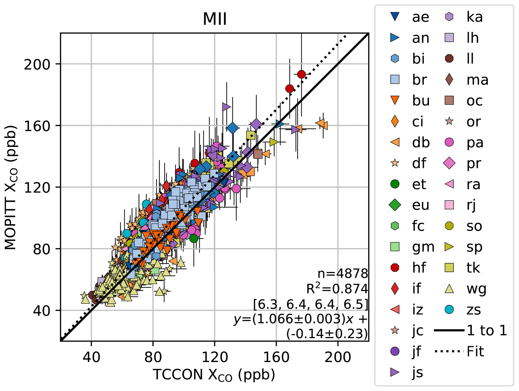
Figure 5One-to-one plot comparing MOPITT and TCCON, following method II (similar to Wunch et al., 2011b, Sect. S6). MOPITT data were adjusted to the TCCON a priori profile (), and MOPITT averaging kernels were applied to TCCON data (). Error bars represent standard deviations of the weighted averages. Triangles represent soundings over water, and other shapes are over land. Text is number of points or days n; coefficient of determination for ordinary least-squares regression R2; and bias (in %) at 50, 75, 100, and 150 ppb using the shown fit and equation for the shown fit using the methods of York et al. (2004).
Figure 6 shows boxplots of the MOPITT to TCCON differences (using method II) for each site for land-only and water-only soundings. We do not note an overall bias between land and water. For all sites the TCCON−MOPITT bias is positive and usually on the order of about 3–10 ppb with a few exceptions. For example, MOPITT observations compared to the AFRC (df) TCCON are particularly high (∼14 ppb). This could be related to the high albedo or high surface temperatures of this desert site.

Figure 6Boxplots of the MOPITT–TCCON percent difference at the TCCON sites (using method II), ordered by latitude (degrees north in parenthesis). Blue boxes are MOPITT soundings over water, and brown boxes are those over land. Whiskers represent the inner 95 % of data. Notches are 95 % confidence intervals of the median. Box heights represent the relative number of observations. The solid horizontal line is the Equator, dashed lines are , and the dotted line is 60∘ N.
4.3 Systematic biases
A seasonal variation in bias may be indicative of differences in sensitivities between the instruments to some feature, such as airmass or water content, that varies seasonally. Figure 7 shows the time series of the difference averaged in 1-month 5∘ latitudinal bands. Though there is significant scatter among individual comparisons, we find a long-term trend of % yr−1 in the MOPITT–TCCON difference using the Theil–Sen estimator. Deeter et al. (2017) reported a bias drift of % yr−1 for V7J, though bias drifts for individual layers were larger. Including a correction trend to the L1 radiances significantly reduced the bias drift for the layers (Deeter et al., 2019). Seasonalities of the difference for each site are in Fig. S14. There does not appear to be a persistent seasonal trend for all sites, though there is some seasonal variability for individual sites. For Lamont and AFRC the bias is larger in July–October, while for Białystok the bias is larger in April–June. At Ascension the bias is largest in January–February, while for Réunion it is largest in September–November. We do not make a seasonal bias correction.
There appears to be some latitudinally dependent bias, with a larger bias in the Northern Hemisphere. Part of this could be related to stratospheric CO (Sect. S1). Deeter et al. (2017) also showed some latitudinal variation in MOPITT retrievals compared with aircraft. They suggested that part of the variability could arise from interfering species such as N2O, which has spectral lines that overlap with the TIR channels. Before V7 a constant value of N2O was assumed, which was determined to cause biases on the order of a few parts per billion (Deeter et al., 2017). In V7 a global average is used based on a linear fit to monthly in situ observations. Figure S14 shows the bias as a function of column N2O measured by the TCCON. There is a slope of , though the overall correlation is small (R2=0.08). There also appears to be a small dependence on column H2O, which was likely reduced in V8 (Deeter et al., 2019). We do not make bias corrections for any of these systematic features.
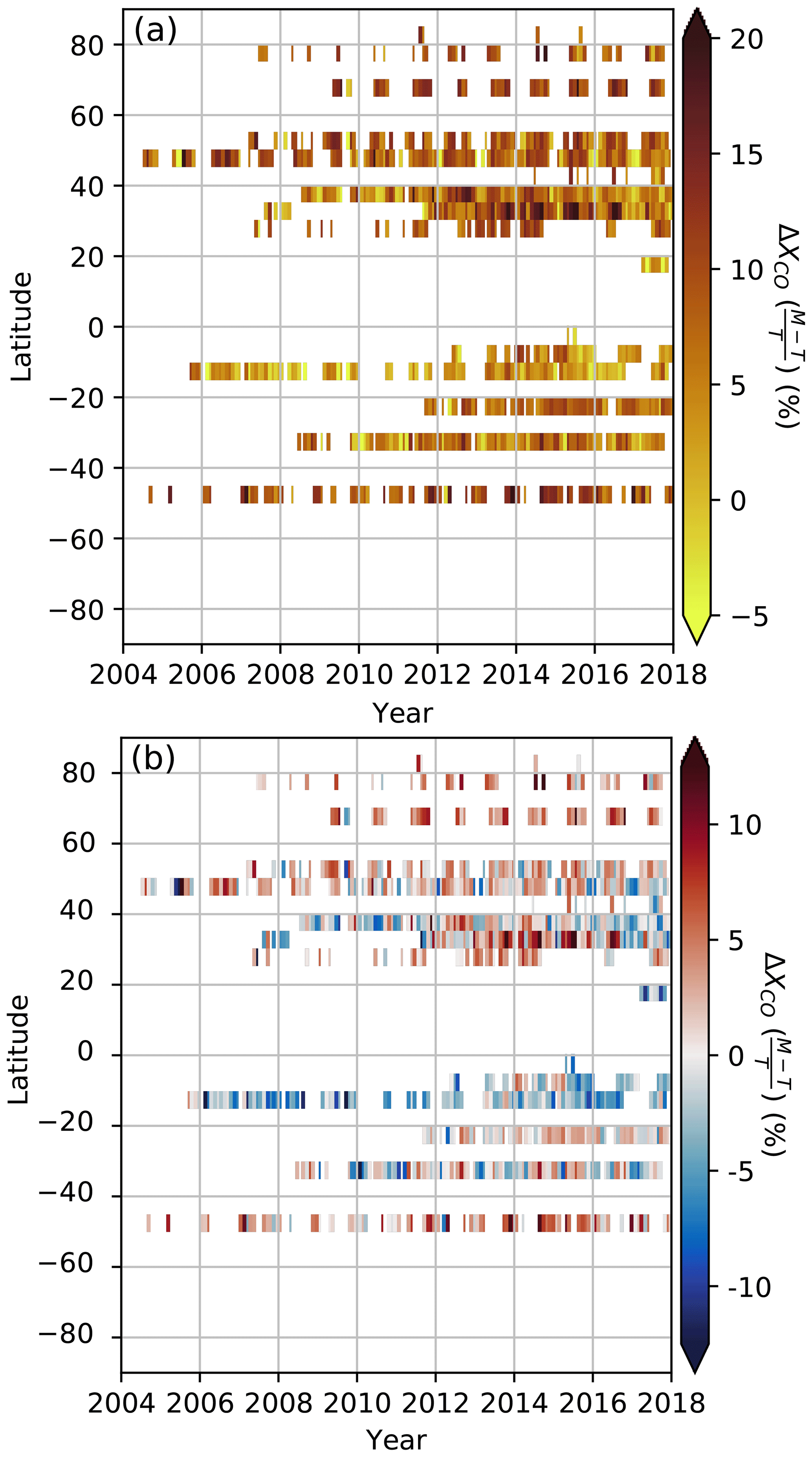
Figure 7Rotated Hovmöller diagram of the mean percent differences between binned MOPITT and TCCON data using method II (Sect. S6.1). Latitude bins are 5∘ zonal bands, and temporal bins are monthly; (a) uses standard TCCON data, and (b) is without the TCCON scaling to aircraft (WMO scale – see Sect. S2).
4.4 Averaging kernels, covariance matrices, and information content
According to Rodgers and Connor (2003, Sect. 2 therein), an intercomparison of two observing systems should also include a comparison of (1) averaging kernels, (2) retrieval noise covariance, (3) degrees of freedom, and (4) the Shannon information content. In conjunction with the comparison of averaging kernels, we think that it is also helpful to compare a priori profiles, which is done in Appendix D. Because the MOPITT retrievals are of logarithmic profiles and the TCCON uses a linear scaling retrieval, some aspects of the comparison are inherently different.

Figure 8Examples of AKs from TCCON and MOPITT – subplots are not always related. MOPITT daytime AKs (a–d) are shown as center-point values along the y axis for clarity, though MOPITT retrievals are layer averages. Unitless MOPITT column AKs are generated using the methods of Appendix B. (a) MOPITT column AKs around Lamont for 2012–2013 separated by pixel. Filled areas are the central 80 %, and solid center lines are the medians per level. Black lines are select examples from single soundings that show wide variability from sounding to sounding. The thicker example corresponds to the full AK in (b). (b) Example MOPITT full AK from 16 October 2012. Dots highlight the ith level shown in the legend. (c) Median MOPITT column AK per level by month for Pasadena. (d) Median MOPITT column AK per level by season for land and water soundings for Lauder. (e) Standard TCCON GGG2014 AKs, which are assumed to be a function of only SZA and pressure. (f) Differences from AKs explicitly calculated at the ETL site on specific days compared to the standard AKs. For 18 June 2017, the mean of the ETL XCO is 74.0±0.8 ppb (1σ). For 9 September 2017, the mean of the ETL XCO is 169±32 ppb (1σ), with a range of 95–225 ppb.
Example AKs for MOPITT and TCCON are shown in Fig. 8. Because the MOPITT retrieval is on a log scale, we make an assumption that the a priori VMRs represent the true profile to obtain unitless AKs (Appendix B). We find that the TCCON AKs are more sensitive than MOPITT. Shaded regions in Fig. 8a show a wide variability in MOPITT column AKs. In addition, the typical state significantly affects the MOPITT AKs (e.g., compare Pasadena and Lauder). TCCON CO column AKs are most sensitive to the stratosphere and are assumed to be consistent at all sites. We make a sensitivity test where the AKs were explicitly calculated in GGG2014 for days with a wide range of XCO at the East Trout Lake site. In general the difference from the standard AKs is small, on the order of 5 % at most.
A priori profiles and MOPITT retrieved profiles along with their differences for select sites are shown in Appendix D. We compare MOPITT and TCCON a priori profiles. In general, MOPITT a priori profiles are influenced more by localized emissions, as they are based on 1∘ simulated monthly climatologies from the CAM-chem model (Deeter et al., 2014). This can be seen especially at Pasadena and to a lesser extent at Lamont and Tsukuba. Ascension Island shows a special case where enhanced CO in the lower free troposphere is seen coming from biomass burning and rainforest VOC emissions in Africa. At sites far removed from local emissions (e.g., Ny-Ålesund and Lauder) the MOPITT and TCCON a priori profiles are in better agreement with each other (see e.g., Pollard et al., 2017).
We take differences in a priori profiles and averaging kernels into account following method II, described in Sect. S6.1. Corrections are applied to each MOPITT retrieval and to daily averages of TCCON retrievals within coincidence criteria. We find in practice that corrections change the comparison by about 3 %. TCCON data are adjusted by 0.7±1.8 ppb (1σ), and MOPITT data are adjusted by ppb (1σ).
Rather than comparing the retrieval noise covariance, we compare reported errors and measures of precision and accuracy. Histograms of total reported retrieval error for MOPITT are shown in Figs. S4o and S5o. With our prescribed filtering, global mean uncertainty values are 2.60±1.27 ppb (1σ) for smoothing, 2.68±1.40 ppb (1σ) for measurement, and 3.86±1.63 ppb (1σ) for the total error. The average of the errors reported in the TCCON files is 0.62±0.50 ppb (1σ). However, these errors are more a measure of repeatability than the total error or the accuracy. The 2σ uncertainty for TCCON (GGG2009) was reported as 4 ppb (Wunch et al., 2010), and the uncertainty budget from a range of sensitivity tests is less than 4 % (Wunch et al., 2015).
Histograms of the MOPITT DOF for the signal for water and land are shown in Figs. S4d and S5k. The DOF for the signal (ds) can be determined from
where ℰ is the expected value operator (Rodgers, 2000, Eq. 2.46 therein). However, ds is usually determined from the trace of the averaging-kernel matrix (Rodgers, 2000, Eq. 2.80 therein), which is equivalent to Eq. (5) for profile retrievals. Because GGG2014 is a scaling retrieval, we treat TCCON measurements as having ds=1. With a profile retrieval we would expect ds>1, as was the case for CO2 (Connor et al., 2016). The DOF gives an indication of how many independent parameters can be improved compared with the a priori profile. MOPITT DOFs are between 1 and 2, which indicates that total column measurements may be reasonable, but individual layer measurements may not always be accurate.
Finally, the information content Hs is a measure of how accurate a measurement is to how well a value is known a priori. Rodgers (2000) expresses it on a natural log scale (Eqs. 2.73 and 2.80 therein):
where In is the identity matrix. Here we express Hs on a log 2 scale instead. Histograms of Hs for MOPITT profile retrievals are shown in Figs. S6a and S8a, and values are on the order of 2.5–5.5 bits over water and 2.5–7 bits over land. If model values of XCO are accurate to about 32 ppb, and if the TCCON accuracy is about 4 ppb, then the TCCON XCO information content is about bits.
We assimilate MOPITT observations using the GEOS-Chem model to show how filtering and the bias correction affect estimated emissions inferred from inversion analyses. We conducted three experiments in which we assimilated the following datasets: (1) the original MOPITT data, (2) the filtered and bias-corrected data with scaling down by about 6 % to match the standard TCCON data (Fig. 5; referred to as Assim. 2), and (3) the filtered and bias-corrected data with a scaling of less than 0.5 % to the TCCON-based data not tied to the WMO scale and without the empirical airmass correction (Fig. S12g; referred to as Assim. 3). The assimilation is performed using the GEOS-Chem four-dimensional variational (4D-Var) data assimilation system, employing Version 35J of the adjoint model at a horizontal resolution of . The GEOS-Chem 4D-Var system has been used in previous studies for assimilation of MOPITT data (e.g., Kopacz et al., 2010; Jiang et al., 2013, 2015, 2017). We assimilate the MOPITT data to optimize monthly average CO emissions. We assimilate daytime observations for the periods of October–December 2009 and May–July 2011 to coincide with flights from the HIPPO campaign. The a posteriori CO fluxes are compared with the a priori fluxes, and the a posteriori CO concentrations are validated against CO measurements from the HIPPO 10 s merged data (Santoni et al., 2014).
The assimilation uses the offline CO simulation in GEOS-Chem with prescribed monthly mean OH fields from TransCom (Patra et al., 2011) to compute the sink of CO. The prior anthropogenic CO emissions are from the EDGAR v4.2 inventory, which are overwritten regionally with the following inventories: the Streets 2006 emissions over China and southeastern Asia from Zhang et al. (2009), the annual Canadian anthropogenic emissions from the Criteria Air Contaminants (CAC inventory), the National Emissions Inventory 2005 (NEI2005) from the United States Environmental Protection Agency (EPA), the “co-operative programme for monitoring and evaluation of the long-range transmission of air pollutants in Europe” (EMEP) inventory, and the Big Bend Regional Aerosol and Visibility Observational (BRAVO) inventory in Mexico. The Global Fire Emissions Database, Version 3 (GFED3), provides the biomass emissions. The biofuel emissions are the Yevich and Logan (2003) inventory. The initial condition of CO states is generated by spinning up the GEOS-Chem model from January 2009. The initial CO concentrations are not optimized in the assimilation. The prior emissions are scaled by a factor of 1.5, and the emission error is purposely set to be 500 % so that the posterior CO source estimates will be less influenced by the a priori emissions and more strongly reflect the information from the filtered MOPITT observations.
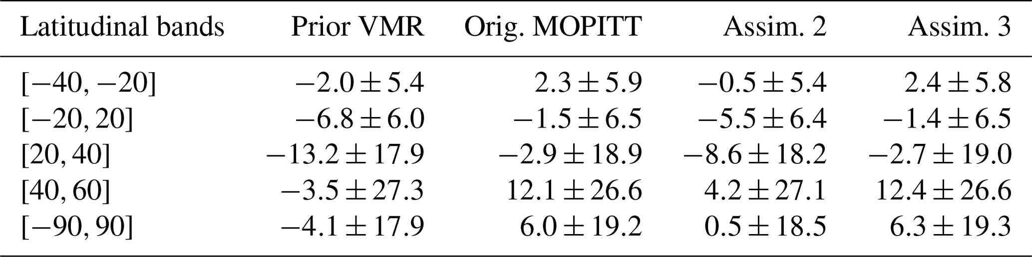
Using HIPPO-2 and HIPPO-4 measurements for comparison, the simulation using only a priori fluxes produces mole fractions that are low by approximately 5 % (Tables 4 and 5). On the other hand, the original MOPITT assimilation and the assimilation which is not tied to WMO (Assimilation 3) tend to agree with each other and are biased high relative to HIPPO measurements. Assimilation 2 mole fractions are lower compared to HIPPO than the other assimilations. This suggests that scaling down MOPITT observations to match TCCON is translated to less CO in the assimilation, as expected. However, the comparison with HIPPO shows mixed results with each simulation depending on which latitudinal bands is considered.
Table 4Comparisons of GEOS-Chem-simulated mole fractions assimilating MOPITT data with HIPPO-2 observations. Uncertainties are 1σ. Units are in parts per billion. See text for descriptions of the assimilations.
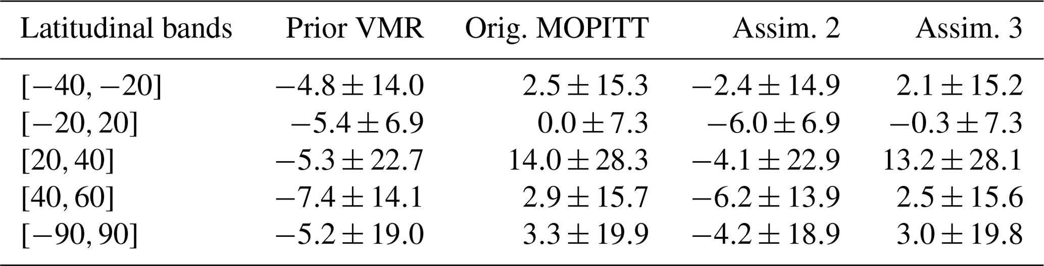
Table 5Comparisons of GEOS-Chem-simulated mole fractions assimilating MOPITT data with HIPPO-4 observations. Uncertainties are 1σ. Units are in parts per billion. See text for descriptions of the assimilations.
To validate the quality of the filtered and bias-corrected MOPITT observations, the prior CO fluxes are compared with the a posteriori fluxes (Fig. 9). Again we find that assimilations 1 and 3 are in general agreement and Assimilation 2 produces lower fluxes. Fluxes using assimilated data are nearly always smaller than fluxes using the prior fluxes scaled up by 50 %. Assimilation 2, which includes scaling MOPITT to the standard TCCON product, produces fluxes that are in between the unscaled (lower) and scaled (higher) prior fluxes. Though fluxes from Assimilation 2 are closest to the unscaled prior fluxes, they are higher by about 30 % and 15 % during HIPPO-2 and HIPPO-4, respectively.
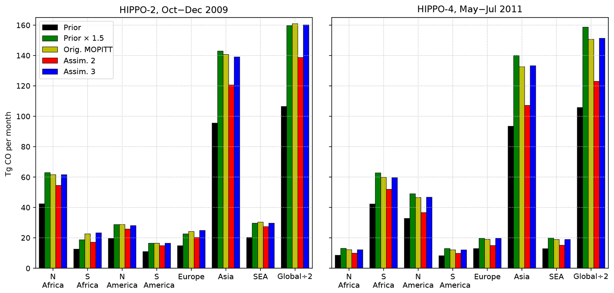
Figure 9Emission estimates from assimilations in GEOS-Chem adjoint model for two different times. For this figure, global emissions are scaled down by 2. SEA is southeastern Asia.
These results are inconclusive as to which of the assimilations is best. Comparisons with HIPPO mole fractions are mixed, and uncertainties in the assimilated prior fluxes prevent us from drawing definitive conclusions from the flux comparison. It is unclear if the filtering and bias corrections improved fluxes in these experiments.
6.1 Practical considerations in intercomparisons of remote sounding retrievals
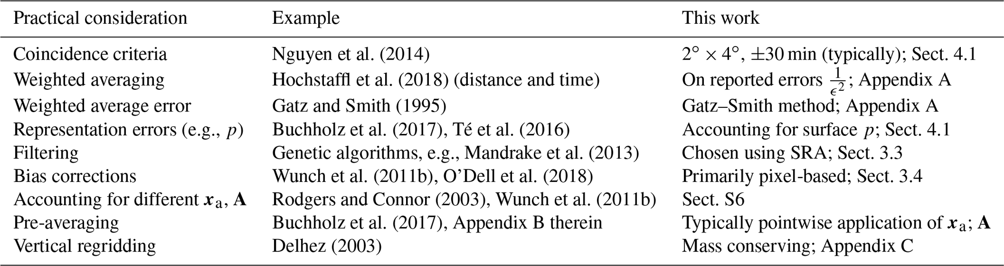
In addition to the formal aspects of intercomparing retrievals from different remote sounding retrievals, there are a variety of practical aspects to consider. For several of these aspects, an entire study could be devoted to them for each intercomparison. We summarize our comparison methodology in Table 6 and give examples of other studies that provide additional details or alternative methods. Though it is impractical to test all combinations of different considerations, we test some as described in Sect. 4.2, such as coincidence criteria, filtering, bias corrections, and applications of averaging kernels.
Nguyen et al. (2014)Hochstaffl et al. (2018)Gatz and Smith (1995)Buchholz et al. (2017)Té et al. (2016)Mandrake et al. (2013)Wunch et al. (2011b)O'Dell et al. (2018)Rodgers and Connor (2003)Wunch et al. (2011b)Buchholz et al. (2017)Delhez (2003)Table 6Summary of practical considerations comparing MOPITT and TCCON soundings.
6.2 Considerations for future MOPITT data use
Several lessons learned in this study may be useful for future versions of MOPITT data products or users assimilating the data. Additional fields used in the retrieval, such as the a priori mixing ratio from 50 to 0 hPa and the water vapor profile, would be useful outputs when converting mixing ratios from whole air to dry air. Though the prior covariance matrix is fixed (Deeter et al., 2010), a single matrix per daily file may be helpful. The retrieved surface emissivity over land is on average about 0.007, or about 0.75 % larger than the prior emissivity, and the retrieved surface temperature is on average about 6 K larger than the prior temperatures (see histograms in Fig. S5f and S5m). This suggests that prior surface emissivity and temperature values should perhaps be reconsidered, as they may be biased low over land. Further updates to prior values of CO, N2O, and H2O are expected to further improve the retrievals. For example, the retrieved column CO is slightly larger than the a priori column globally (Fig. S16), but the difference depends on the level and could be related to uncertainties in model transport, sinks, and sources.
Filtering can reduce spurious values. MOPITT files include parameters that could be used in filtering, such as a retrieval anomaly diagnostic, various cloud indicators, and the DOF. Data users should consider creating a QC flag for their analyses, or a binary flag could be included in future versions, e.g., based on parameters in Table 3 or based on the recommendations of the MOPITT team (e.g., the L3 filters). Often highly deviant retrieved surface temperatures show up around coastlines (especially western coastlines; Fig. S10) that did not pass our quality screening. These may be related to sounding definitions of surface type. SNR 6A is used to filter MOPITT data when creating the TIR–NIR L3 product to maintain consistency with the NIR product and increase stability of the DOF, but we do not find sufficient evidence to use it as a TIR–NIR filter criterion based on XCO stability alone.
When biases are found in the MOPITT L2 data, the strategy is to correct the L1 radiances or the retrieval algorithm (e.g., Deeter et al., 2019). MOPITT data users of L2 XCO may consider implementing a bias correction before analysis or model assimilation. In terms of XCO, pixel-3 data agree with pixels 2 and 4; however, this agreement may not necessarily hold for retrieved profiles, and pixel-3 data are excluded in the L3 product due to excessive NIR noise and in order to increase stability in the DOF (e.g., Deeter et al., 2015). A bias correction should be considered when assimilating pixel 1. There is a bias in the SRA for large retrieval errors on XCO above about 8 ppb (Figs. S4o, S5o). This bias suggests that perhaps these data should be excluded or deweighted further, which we did not do here. A bias adjustment field could also be included as a field in future MOPITT files. Such an adjustment could account for empirical biases noted with various parameters; pixel-to-pixel biases (Sect. 3.4); and an overall bias compared with NDACC (Buchholz et al., 2017), aircraft flights (Deeter et al., 2017), and/or TCCON.
In this study quality-filtered and bias-corrected MOPITT data are compared with TCCON data. We first derive filters using only the MOPITT data, assuming homogeneity over small regions. These filters have the largest effectover snow or ice scenes and over high terrain. They reduce the overall RMS from 3.84 to 2.55 ppb. We find and correct a bias among the four pixels, which we confirmed exists using AirCore. We also find and correct a feature bias.
After the filtering and bias correction, we compare with TCCON data. Using a method (method II; see Sect. S6.1) similar to Wunch et al. (2011b) to account for differences in a priori profiles and AKs, we find MOPITT data to be biased high by about 6 % compared with TCCON, but it is not clear whether MOPITT or TCCON is biased. We also test different methods, which all lead to a bias of about 6 %–10 %. There is a trend of % yr−1 in the MOPITT–TCCON difference. The bias also appears to depend on site and latitude, but the scatter is not consistent enough to derive a correction. We also compared AKs and information content from the different retrievals. TCCON AKs are more sensitive to changes in the stratosphere. MOPITT AKs peak in the mid-troposphere and can vary significantly among locations.
After applying filtering, and an overall scaling to match the TCCON, we assimilate the data into GEOS-Chem. Filtering and bias correction are uniform enough to not make a large difference among regional fluxes. When data are also scaled down to TCCON before implementing into GEOS-Chem, fluxes were lower in all regions. However, because of bottom-up uncertainties in global CO fluxes, these experiments were inconclusive. Additional work is needed to understand the relatively large (∼6 %) difference between MOPITT and TCCON.
MOPITT data were obtained from the NASA Langley server (ftp://l5ftl01.larc.nasa.gov/MOPITT/, last access: 12 December 2018). TCCON data were obtained through the TCCON data archive hosted by CaltechDATA (TCCON, 2018). See Table 1 for data references for each site. TCCON data without the scaling to the WMO scale were obtained from the site PIs. AirCore data were obtained from Colm Sweeney (v20170918).
The MOPITT V7 data product contains fields for retrieved total column CO (in molec. cm−2). Unlike the TCCON, MOPITT does not retrieve a dry-air column. However, a model dry-air column is provided. We obtain a dry-air mole fraction from
The retrieval error (in molec. cm−2) can be converted to parts per billion in the same way.
When averaging n soundings together, we use a weighted average using the inverse squared retrieval errors as weights. The average retrieved value is
where denotes an individual measurement in the bin, and is the corresponding error. When an average weighted error is needed, we calculate a weighted standard error of the mean (SEM) using
In the case of uniform weights , this reduces to the typical SEM equation. We also test a bootstrap analysis (Efron and Gong, 1983) on binned data for one of the parameters (DEsfc) in the bias correction analysis (Sect. 3.4) to evaluate Eq. (A3). Data are placed into 146 bins, with at least 2000 points in each. The bootstrap is run 500 times per bin. We find, in agreement with Gatz and Smith (1995), that Eq. (A3) is a reasonable approximation to the SEM determined from the bootstrap method, with an offset of only % (1σ).
We derive our own MOPITT column-averaging-kernel (AK) vector based on the full averaging-kernel matrix. To fulfill Eq. (2) (and using Eq. 4), MOPITT AK elements aj are
Making use of , and ,
This MOPITT column-averaging kernel is not directly comparable with the TCCON column-averaging kernels because of the log scale. A unitless column-averaging kernel can be made but requires an a priori assumption about the true state of the atmosphere. For example,
We find it necessary to express values from one retrieval on the vertical pressure grid of the other. MOPITT profiles are reported as layer averages, but TCCON profiles are reported as level values. TCCON profiles are converted to the MOPITT grid by linear interpolation. We divide each MOPITT layer into 500 finer equal-pressure layers (about 0.4 hPa each). We interpolate the TCCON profiles to these finer layers and then take the overall average to put the TCCON profile on the MOPITT pressure grid.
Basic interpolation on the midpoints should not be used to convert the MOPITT layer averages to the TCCON grid because it does not require that mass be conserved when the layers have different widths. Instead we use a mass-conserving linear-interpolation scheme based on the MOPITT layer averages. This is based on the work of Hedelius and Wunch (2019) and Delhez (2003).
The a priori profiles differ between MOPITT and TCCON. This could lead to different intercomparison results depending on which is chosen as a comparison ensemble. In general, the TCCON a priori profiles are smooth, with only 3-D variation (time, latitude, and altitude) that takes into account the local tropopause height. MOPITT a priori profiles are 4-D (time, latitude, longitude, and altitude) and hence differ in locations with strong local pollution (e.g., Pasadena). Examples of prior and retrieved profiles and their differences for several sites are in Fig. D1. Global maps of the average ratios between the retrieved and prior values for MOPITT are available in Sect. S9.
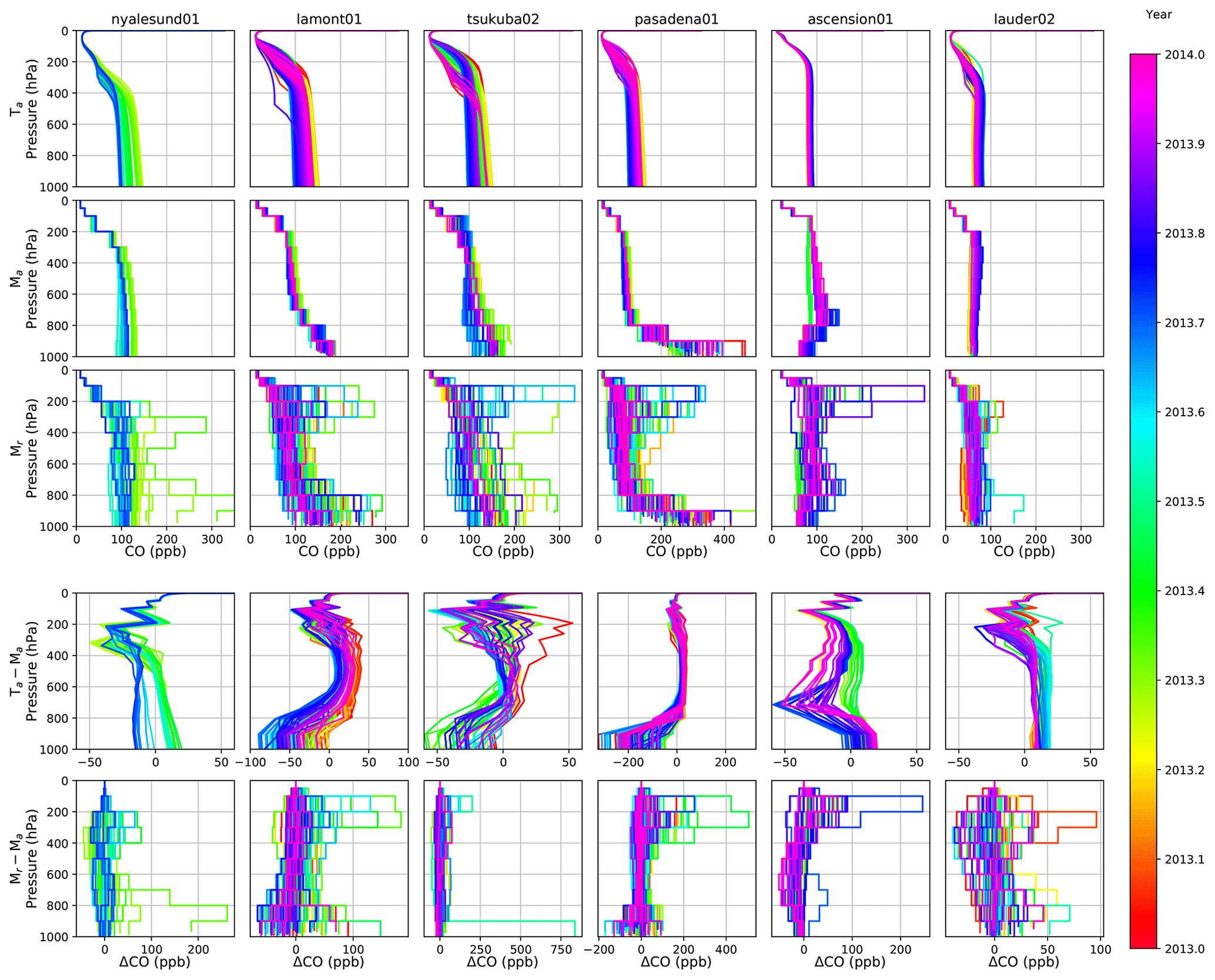
Figure D1Profiles and profile differences between MOPITT and TCCON for six select sites and different days in 2013. For clarity, only one MOPITT profile within the coincidence criteria is selected per day. The rows are the TCCON a priori profiles (Ta), the MOPITT a priori profiles (Ma), the MOPITT retrieved profiles (Mr), the difference between TCCON and MOPITT a priori profiles, and the difference between MOPITT a priori and retrieved profiles.
The supplement related to this article is available online at: https://doi.org/10.5194/amt-12-5547-2019-supplement.
JKH and DW were involved in the overall conceptualization, investigation, and methodology development. DW secured funding and computational resources and provided supervision. TLH wrote the original Sect. 5 draft. JKH did the formal analysis and visualization and wrote the remainder of the original draft. TLH and DBAJ created methodology for and performed the GEOS-Chem assimilations and comparisons with HIPPO data. CS and BCB provided the AirCore data, and MDM, NMD, MKD, DGF, DWTG, FH, LTI, PJ, MK, RK, CL, IM, JN, YSO, HO, DFP, MR, SR, CMR, MS, K Shiomi, K Strong, RS, YT, OU, VAV, WW, TW, POW, and DW provided the TCCON data, which involves independent funding acquisition, site management, data acquisition and processing, QA/QC (quality assurance/quality control), and delivery. RRB and HMW provided guidance on MOPITT data and insight into the MOPITT instrument, algorithm, and previous validation results. JKH, DW, DBAJ, RRB, NMD, FH, MK, IM, JN, RS, POW, HMW, CS, and BCB reviewed the paper. JKH and DW implemented edits to the paper.
The authors declare that they have no conflict of interest.
This project is undertaken with the financial support of the Canadian Space Agency (CSA) through the Earth System Science Data Analyses program (grant no. 16SUASCOBF).
This paragraph contains TCCON site acknowledgements as requested by site PIs and co-authors. The Ascension Island TCCON station has been supported by the European Space Agency (ESA) under grant no. 3-14737 and by the German Bundesministerium für Wirtschaft und Energie (BMWi) under grant nos. 50EE1711C and 50EE1711E. We thank the ESA Ariane tracking station at North East Bay, Ascension Island, for hosting and local support. The Four Corners and Manaus TCCON stations have been supported by LANL-LDRD. The Eureka TCCON measurements were made at the Polar Environment Atmospheric Research Laboratory (PEARL) by the Canadian Network for the Detection of Atmospheric Change (CANDAC), primarily supported by the CSA, NSERC, and Environment and Climate Change Canada (ECCC). The East Trout Lake TCCON station is supported by the Canada Foundation for Innovation, the Ontario Research Fund, and ECCC. Work at Anmyeondo was funded by Korea Meteorological Administration Research and Development Program “Research and Development for KMA Weather, Climate, and Earth System Services” under grant KMA2018-00321. The TCCON projects for Rikubetsu, Tsukuba, and Burgos sites are supported in part by the GOSAT series project. Site support for Burgos is provided by the Energy Development Corporation (EDC, Philippines). Nicholas M. Deutscher is supported by an ARC Future Fellowship, FT180100327.
We thank the MOPITT team for providing the MOPITT data – especially Merritt Deeter and James Drummond for helpful discussions. We thank Geoff Toon for developing the GGG2014 code used to process the TCCON data. We acknowledge the TCCON co-investigators and site technicians who have also helped maintain sites and provide data throughout the years as well as the respective funding organizations that supported the TCCON measurements at the various sites. Specifically we acknowledge Thomas Blumenstock, Youwen Sun, Joseph Mendonca, and Tae-Young Goo.
We thank Roisin Commane, Enrico Dammers, Benjamin Gaubert, Junjie Liu, Anna Michalak, Charles Miller, Katherine Saad, Mahesh Sha, and Felix Vogel for helpful discussions. We especially thank Merritt Deeter, John Gille, and Geoff Toon for providing feedback on the paper.
We thank Chris O'Dell and one anonymous reviewer for reviewing this paper. We thank Andre Butz for serving as editor.
This research has been supported by the Canadian Space Agency (grant no. 16SUASCOBF), the European Space Agency (grant no. 3-14737), the Bundesministerium für Wirtschaft und Energie (grant no. 50EE1711C), the Los Alamos National Laboratory (grant no. LANL-LDRD), the Korea Meteorological Administration (grant no. KMA2018-00321), the Japan Aerospace Exploration Agency (grant no. GOSAT series), and the Australian Research Council (grant no. FT180100327).
This paper was edited by Andre Butz and reviewed by Christopher O'Dell and one anonymous referee.
Blumenstock, T., Hase, F., Schneider, M., Garcia, O. E., and Sepulveda, E.: TCCON data from Izana (ES), Release GGG2014R0, TCCON data archive, CaltechDATA, https://doi.org/10.14291/tccon.ggg2014.izana01.R0/1149295, 2014. a
Borsdorff, T., aan de Brugh, J., Hu, H., Hasekamp, O., Sussmann, R., Rettinger, M., Hase, F., Gross, J., Schneider, M., Garcia, O., Stremme, W., Grutter, M., Feist, D. G., Arnold, S. G., De Mazière, M., Kumar Sha, M., Pollard, D. F., Kiel, M., Roehl, C., Wennberg, P. O., Toon, G. C., and Landgraf, J.: Mapping carbon monoxide pollution from space down to city scales with daily global coverage, Atmos. Meas. Tech., 11, 5507–5518, https://doi.org/10.5194/amt-11-5507-2018, 2018. a
Buchholz, R. R., Deeter, M. N., Worden, H. M., Gille, J., Edwards, D. P., Hannigan, J. W., Jones, N. B., Paton-Walsh, C., Griffith, D. W. T., Smale, D., Robinson, J., Strong, K., Conway, S., Sussmann, R., Hase, F., Blumenstock, T., Mahieu, E., and Langerock, B.: Validation of MOPITT carbon monoxide using ground-based Fourier transform infrared spectrometer data from NDACC, Atmos. Meas. Tech., 10, 1927–1956, https://doi.org/10.5194/amt-10-1927-2017, 2017. a, b, c, d, e, f, g, h, i, j, k, l, m, n
Connor, B. J., Boesch, H., Toon, G., Sen, B., Miller, C., and Crisp, D.: Orbiting Carbon Observatory: Inverse method and prospective error analysis, J. Geophys. Res., 113, D05305, https://doi.org/10.1029/2006JD008336, 2008. a
Connor, B. J., Sherlock, V., Toon, G., Wunch, D., and Wennberg, P. O.: GFIT2: an experimental algorithm for vertical profile retrieval from near-IR spectra, Atmos. Meas. Tech., 9, 3513–3525, https://doi.org/10.5194/amt-9-3513-2016, 2016. a
De Mazière, M., Sha, M. K., Desmet, F., Hermans, C., Scolas, F., Kumps, N., Metzger, J.-M., Duflot, V., and Cammas, J.-P.: TCCON data from Reunion Island (RE), Release GGG2014R0, TCCON data archive, CaltechDATA, https://doi.org/10.14291/tccon.ggg2014.reunion01.R0/1149288, 2014. a
Deeter, M. N.: MOPITT (Measurements of Pollution in the Troposphere), Version 7, Product User's Guide, available at: https://www2.acom.ucar.edu/sites/default/files/mopitt/v7_users_guide_201707.pdf (last access: 16 August 2018), 2017. a, b
Deeter, M. N., Edwards, D. P., Gille, J. C., Emmons, L. K., Francis, G., Ho, S. P., Mao, D., Masters, D., Worden, H., Drummond, J. R., and Novelli, P. C.: The MOPITT version 4 CO product: Algorithm enhancements, validation, and long-term stability, J. Geophys. Res., 115, D07306, https://doi.org/10.1029/2009jd013005, 2010. a, b
Deeter, M. N., Martínez-Alonso, S., Edwards, D. P., Emmons, L. K., Gille, J. C., Worden, H. M., Sweeney, C., Pittman, J. V., Daube, B. C., and Wofsy, S. C.: The MOPITT Version 6 product: algorithm enhancements and validation, Atmos. Meas. Tech., 7, 3623–3632, https://doi.org/10.5194/amt-7-3623-2014, 2014. a, b, c, d, e, f
Deeter, M. N., Edwards, D. P., Gille, J. C., and Worden, H. M.: Information content of MOPITT CO profile retrievals: Temporal and geographical variability, J. Geophys. Res.-Atmos., 120, 12723–12738, https://doi.org/10.1002/2015JD024024, 2015. a, b, c, d, e
Deeter, M. N., Martínez-Alonso, S., Gatti, L. V., Gloor, M., Miller, J. B., Domingues, L. G., and Correia, C. S. C.: Validation and analysis of MOPITT CO observations of the Amazon Basin, Atmos. Meas. Tech., 9, 3999–4012, https://doi.org/10.5194/amt-9-3999-2016, 2016. a, b, c
Deeter, M. N., Edwards, D. P., Francis, G. L., Gille, J. C., Martínez-Alonso, S., Worden, H. M., and Sweeney, C.: A climate-scale satellite record for carbon monoxide: the MOPITT Version 7 product, Atmos. Meas. Tech., 10, 2533–2555, https://doi.org/10.5194/amt-10-2533-2017, 2017. a, b, c, d, e, f, g, h, i, j
Deeter, M. N., Edwards, D. P., Francis, G. L., Gille, J. C., Mao, D., Martínez-Alonso, S., Worden, H. M., Ziskin, D., and Andreae, M. O.: Radiance-based retrieval bias mitigation for the MOPITT instrument: the version 8 product, Atmos. Meas. Tech., 12, 4561–4580, https://doi.org/10.5194/amt-12-4561-2019, 2019. a, b, c, d
Delhez, E.: A spline interpolation technique that preserves mass budgets, Appl. Math. Lett., 16, 17–26, https://doi.org/10.1016/S0893-9659(02)00139-8, 2003. a, b
Deutscher, N. M., Notholt, J., Messerschmidt, J., Weinzierl, C., Warneke, T., Petri, C., Grupe, P., and Katrynski, K.: TCCON data from Bialystok (PL), Release GGG2014R1, TCCON data archive, CaltechDATA, https://doi.org/10.14291/tccon.ggg2014.bialystok01.R1/1183984, 2014. a
Drummond, J. R., Zou, J., Nichitiu, F., Kar, J., Deschambaut, R., and Hackett, J.: A review of 9-year performance and operation of the MOPITT instrument, Adv. Space Res., 45, 760–774, https://doi.org/10.1016/j.asr.2009.11.019, 2010. a, b, c
Dubey, M., Henderson, B., Green, D., Butterfield, Z., Keppel-Aleks, G., Allen, N., Blavier, J.-F., Roehl, C., Wunch, D., and Lindenmaier, R.: TCCON data from Manaus (BR), Release GGG2014R0, TCCON data archive, CaltechDATA, https://doi.org/10.14291/tccon.ggg2014.manaus01.R0/1149274, 2014a. a
Dubey, M., Lindenmaier, R., Henderson, B., Green, D., Allen, N., Roehl, C., Blavier, J.-F., Butterfield, Z., Love, S., Hamelmann, J., and Wunch, D.: TCCON data from Four Corners (US), Release GGG2014R0, TCCON data archive, CaltechDATA, https://doi.org/10.14291/tccon.ggg2014.fourcorners01.R0/1149272, 2014b. a
Efron, B. and Gong, G.: A leisurely look at the bootstrap, the jackknife, and cross-validation, Am. Stat., 37, 36–48, https://doi.org/10.1080/00031305.1983.10483087, 1983. a
Engel, A., Bönisch, H., Ullrich, M., Sitals, R., Membrive, O., Danis, F., and Crevoisier, C.: Mean age of stratospheric air derived from AirCore observations, Atmos. Chem. Phys., 17, 6825–6838, https://doi.org/10.5194/acp-17-6825-2017, 2017. a
Feist, D. G., Arnold, S. G., John, N., and Geibel, M. C.: TCCON data from Ascension Island (SH), Release GGG2014R0, TCCON data archive, CaltechDATA, https://doi.org/10.14291/tccon.ggg2014.ascension01.R0/1149285, 2014. a
Forster, P., Ramaswamy, V., Artaxo, P., Berntsen, T., Betts, R., Fahey, D., Haywood, J., Lean, J., Lowe, D., Myhre, G., Nganga, J., Prinn, R., Raga, G., Schulz, M., and Van Dorland, R.: Changes in Atmospheric Constituents and in Radiative Forcing, in: Climate Change 2007: The Physical Science Basis. Contribution of Working Group I to the Fourth Assessment Report of the Intergovernmental Panel on Climate Change, edited by: Solomon, S., Qin, D., Manning, M., Chen, Z., Marquis, M., K.B., A., Tignor, M., and Miller, H., Cambridge University Press, Cambridge, United Kingdom and New York, USA, chap. 2, 129–234, available at: https://www.ipcc.ch/publications_and_data/ar4/wg1/en/contents.html (last access: 17 January 2019), 2007. a
Gatz, D. F. and Smith, L.: The standard error of a weighted mean concentration – I. Bootstrapping vs other methods, Atmos. Environ., 29, 1185–1193, https://doi.org/10.1016/1352-2310(94)00210-C, 1995. a, b
Goo, T.-Y., Oh, Y.-S., and Velazco, V. A.: TCCON data from Anmeyondo (KR), Release GGG2014R0, TCCON data archive, CaltechDATA, https://doi.org/10.14291/tccon.ggg2014.anmeyondo01.R0/1149284, 2014. a
Griffith, D. W., Deutscher, N. M., Velazco, V. A., Wennberg, P. O., Yavin, Y., Aleks, G. K., Washenfelder, R. a., Toon, G. C., Blavier, J.-F., Murphy, C., Jones, N., Kettlewell, G., Connor, B. J., Macatangay, R., Roehl, C., Ryczek, M., Glowacki, J., Culgan, T., and Bryant, G.: TCCON data from Darwin (AU), Release GGG2014R0, TCCON data archive, CaltechDATA, https://doi.org/10.14291/tccon.ggg2014.darwin01.R0/1149290, 2014a. a
Griffith, D. W., Velazco, V. A., Deutscher, N. M., Murphy, C., Jones, N., Wilson, S., Macatangay, R., Kettlewell, G., Buchholz, R. R., and Riggenbach, M.: TCCON data from Wollongong (AU), Release GGG2014R0, TCCON data archive, CaltechDATA, https://doi.org/10.14291/tccon.ggg2014.wollongong01.R0/1149291, 2014b. a
Hase, F., Blumenstock, T., Dohe, S., Gross, J., and Kiel, M.: TCCON data from Karlsruhe (DE), Release GGG2014R1, TCCON data archive, CaltechDATA, https://doi.org/10.14291/tccon.ggg2014.karlsruhe01.R1/1182416, 2014. a
Hedelius, J. K. and Wunch, D.: Mass conserving quartic-spline and linear interpolation techniques over variable width partitions, Scholars Portal Dataverse, V1, https://doi.org/10.5683/SP2/57ROYV, 2019. a
Hedelius, J. K., Feng, S., Roehl, C. M., Wunch, D., Hillyard, P. W., Podolske, J. R., Iraci, L. T., Patarasuk, R., Rao, P., O'Keeffe, D., Gurney, K. R., Lauvaux, T., and Wennberg, P. O.: Emissions and topographic effects on column CO2 () variations, with a focus on the Southern California Megacity, J. Geophys. Res.-Atmos., 122, 7200–7215, https://doi.org/10.1002/2017JD026455, 2017. a, b
Hochstaffl, P., Schreier, F., Lichtenberg, G., and García, S. G.: Validation of carbon monoxide total column retrievals from SCIAMACHY observations with NDACC/TCCON ground-based measurements, Remote Sensing, 10, 223, https://doi.org/10.3390/rs10020223, 2018. a, b, c, d
Inoue, M., Morino, I., Uchino, O., Nakatsuru, T., Yoshida, Y., Yokota, T., Wunch, D., Wennberg, P. O., Roehl, C. M., Griffith, D. W. T., Velazco, V. A., Deutscher, N. M., Warneke, T., Notholt, J., Robinson, J., Sherlock, V., Hase, F., Blumenstock, T., Rettinger, M., Sussmann, R., Kyrö, E., Kivi, R., Shiomi, K., Kawakami, S., De Mazière, M., Arnold, S. G., Feist, D. G., Barrow, E. A., Barney, J., Dubey, M., Schneider, M., Iraci, L. T., Podolske, J. R., Hillyard, P. W., Machida, T., Sawa, Y., Tsuboi, K., Matsueda, H., Sweeney, C., Tans, P. P., Andrews, A. E., Biraud, S. C., Fukuyama, Y., Pittman, J. V., Kort, E. A., and Tanaka, T.: Bias corrections of GOSAT SWIR XCO2 and XCH4 with TCCON data and their evaluation using aircraft measurement data, Atmos. Meas. Tech., 9, 3491–3512, https://doi.org/10.5194/amt-9-3491-2016, 2016. a
Iraci, L. T., Podolske, J., Hillyard, P. W., Roehl, C., Wennberg, P. O., Blavier, J.-F., Allen, N., Wunch, D., Osterman, G. B., and Albertson, R.: TCCON data from Edwards (US), Release GGG2014R1, TCCON data archive, CaltechDATA, https://doi.org/10.14291/tccon.ggg2014.edwards01.R1/1255068, 2016a. a
Iraci, L. T., Podolske, J., Hillyard, P. W., Roehl, C., Wennberg, P. O., Blavier, J.-F., Landeros, J., Allen, N., Wunch, D., Zavaleta, J., Quigley, E., Osterman, G. B., Barrow, E., and Barney, J.: TCCON data from Indianapolis (US), Release GGG2014R1, TCCON data archive, CaltechDATA, https://doi.org/10.14291/tccon.ggg2014.indianapolis01.R1/1330094, 2016b. a
Jiang, Z., Jones, D. B. A., Worden, H. M., Deeter, M. N., Henze, D. K., Worden, J., Bowman, K. W., Brenninkmeijer, C. A. M., and Schuck, T. J.: Impact of model errors in convective transport on CO source estimates inferred from MOPITT CO retrievals, J. Geophys. Res.-Atmos., 118, 2073–2083, https://doi.org/10.1002/jgrd.50216, 2013. a
Jiang, Z., Jones, D. B. A., Worden, H. M., and Henze, D. K.: Sensitivity of top-down CO source estimates to the modeled vertical structure in atmospheric CO, Atmos. Chem. Phys., 15, 1521-1537, https://doi.org/10.5194/acp-15-1521-2015, 2015. a
Jiang, Z., Worden, J. R., Worden, H., Deeter, M., Jones, D. B. A., Arellano, A. F., and Henze, D. K.: A 15-year record of CO emissions constrained by MOPITT CO observations, Atmos. Chem. Phys., 17, 4565–4583, https://doi.org/10.5194/acp-17-4565-2017, 2017. a
Karion, A., Sweeney, C., Tans, P., and Newberger, T.: AirCore: An innovative atmospheric sampling system, J. Atmos. Ocean. Tech., 27, 1839–1853, https://doi.org/10.1175/2010JTECHA1448.1, 2010. a
Kawakami, S., Ohyama, H., Arai, K., Okumura, H., Taura, C., Fukamachi, T., and Sakashita, M.: TCCON data from Saga (JP), Release GGG2014R0, TCCON data archive, CaltechDATA, https://doi.org/10.14291/tccon.ggg2014.saga01.R0/1149283, 2014. a
Kiel, M., Wunch, D., Wennberg, P. O., Toon, G. C., Hase, F., and Blumenstock, T.: Improved retrieval of gas abundances from near-infrared solar FTIR spectra measured at the Karlsruhe TCCON station, Atmos. Meas. Tech., 9, 669–682, https://doi.org/10.5194/amt-9-669-2016, 2016. a
Kiel, M., O'Dell, C. W., Fisher, B., Eldering, A., Nassar, R., MacDonald, C. G., and Wennberg, P. O.: How bias correction goes wrong: measurement of affected by erroneous surface pressure estimates, Atmos. Meas. Tech., 12, 2241–2259, https://doi.org/10.5194/amt-12-2241-2019, 2019. a
Kivi, R. and Heikkinen, P.: Fourier transform spectrometer measurements of column CO2 at Sodankylä, Finland, Geosci. Instrum. Method. Data Syst., 5, 271–279, https://doi.org/10.5194/gi-5-271-2016, 2016. a
Kivi, R., Heikkinen, P., and Kyrö, E.: TCCON data from Sodankyla (FI), Release GGG2014R0, TCCON data archive, CaltechDATA, https://doi.org/10.14291/tccon.ggg2014.sodankyla01.R0/1149280, 2017. a
Kopacz, M., Jacob, D. J., Fisher, J. A., Logan, J. A., Zhang, L., Megretskaia, I. A., Yantosca, R. M., Singh, K., Henze, D. K., Burrows, J. P., Buchwitz, M., Khlystova, I., McMillan, W. W., Gille, J. C., Edwards, D. P., Eldering, A., Thouret, V., and Nedelec, P.: Global estimates of CO sources with high resolution by adjoint inversion of multiple satellite datasets (MOPITT, AIRS, SCIAMACHY, TES), Atmos. Chem. Phys., 10, 855–876, https://doi.org/10.5194/acp-10-855-2010, 2010. a
Kulawik, S., Wunch, D., O'Dell, C., Frankenberg, C., Reuter, M., Oda, T., Chevallier, F., Sherlock, V., Buchwitz, M., Osterman, G., Miller, C. E., Wennberg, P. O., Griffith, D., Morino, I., Dubey, M. K., Deutscher, N. M., Notholt, J., Hase, F., Warneke, T., Sussmann, R., Robinson, J., Strong, K., Schneider, M., De Mazière, M., Shiomi, K., Feist, D. G., Iraci, L. T., and Wolf, J.: Consistent evaluation of ACOS-GOSAT, BESD-SCIAMACHY, CarbonTracker, and MACC through comparisons to TCCON, Atmos. Meas. Tech., 9, 683–709, https://doi.org/10.5194/amt-9-683-2016, 2016. a
Lamarque, J.-F., Emmons, L. K., Hess, P. G., Kinnison, D. E., Tilmes, S., Vitt, F., Heald, C. L., Holland, E. A., Lauritzen, P. H., Neu, J., Orlando, J. J., Rasch, P. J., and Tyndall, G. K.: CAM-chem: description and evaluation of interactive atmospheric chemistry in the Community Earth System Model, Geosci. Model Dev., 5, 369–411, https://doi.org/10.5194/gmd-5-369-2012, 2012. a
Lelieveld, J., Gromov, S., Pozzer, A., and Taraborrelli, D.: Global tropospheric hydroxyl distribution, budget and reactivity, Atmos. Chem. Phys., 16, 12477–12493, https://doi.org/10.5194/acp-16-12477-2016, 2016. a
Lindenmaier, R., Dubey, M. K., Henderson, B. G., Butterfield, Z. T., Herman, J. R., Rahn, T., and Lee, S.-H.: Multiscale observations of CO2, 13CO2, and pollutants at Four Corners for emission verification and attribution, P. Natl. Acad. of Sci. USA, 111, 8386–8391, https://doi.org/10.1073/pnas.1321883111, 2014. a, b
Liu, C., Wang, W., and Sun, Y.: TCCON data from Hefei, China, Release GGG2014.R0, TCCON data archive, CaltechDATA, https://doi.org/10.14291/tccon.ggg2014.hefei01.R0, 2018. a
Mandrake, L., Frankenberg, C., O'Dell, C. W., Osterman, G., Wennberg, P., and Wunch, D.: Semi-autonomous sounding selection for OCO-2, Atmos. Meas. Tech., 6, 2851–2864, https://doi.org/10.5194/amt-6-2851-2013, 2013. a
Membrive, O., Crevoisier, C., Sweeney, C., Danis, F., Hertzog, A., Engel, A., Bönisch, H., and Picon, L.: AirCore-HR: a high-resolution column sampling to enhance the vertical description of CH4 and CO2, Atmos. Meas. Tech., 10, 2163–2181, https://doi.org/10.5194/amt-10-2163-2017, 2017. a
Morino, I., Matsuzaki, T., and Shishime, A.: TCCON data from Tsukuba (JP), 125HR, Release GGG2014R1, TCCON data archive, CaltechDATA, https://doi.org/10.14291/tccon.ggg2014.tsukuba02.R1/1241486, 2014a. a
Morino, I., Yokozeki, N., Matzuzaki, T., and Horikawa, M.: TCCON data from Rikubetsu (JP), Release GGG2014R1, TCCON data archive, CaltechDATA, https://doi.org/10.14291/tccon.ggg2014.rikubetsu01.R1/1242265, 2014b. a
Morino, I., Velazco, V. A., Hori, A., Uchino, O., and Griffith, D. W. T.: TCCON data from Burgos, Ilocos Norte (PH), Release GGG2014.R0, TCCON data archive, CaltechDATA, https://doi.org/10.14291/tccon.ggg2014.burgos01.R0, 2018. a
Mu, M., Randerson, J. T., van der Werf, G. R., Giglio, L., Kasibhatla, P., Morton, D., Collatz, G. J., DeFries, R. S., Hyer, E. J., Prins, E. M., Griffith, D. W. T., Wunch, D., Toon, G. C., Sherlock, V., and Wennberg, P. O.: Daily and 3-hourly variability in global fire emissions and consequences for atmospheric model predictions of carbon monoxide, J. Geophys. Res., 116, D24303, https://doi.org/10.1029/2011JD016245, 2011. a
Nguyen, H., Osterman, G., Wunch, D., O'Dell, C., Mandrake, L., Wennberg, P., Fisher, B., and Castano, R.: A method for colocating satellite data to ground-based data and its application to ACOS-GOSAT and TCCON, Atmos. Meas. Tech., 7, 2631–2644, https://doi.org/10.5194/amt-7-2631-2014, 2014. a, b
Notholt, J., Petri, C., Warneke, T., Deutscher, N. M., Buschmann, M., Weinzierl, C., Macatangay, R., and Grupe, P.: TCCON data from Bremen (DE), Release GGG2014R0, TCCON data archive, CaltechDATA, https://doi.org/10.14291/tccon.ggg2014.bremen01.R0/1149275, 2014. a
Notholt, J., Warneke, T., Petri, C., Deutscher, N. M., Weinzierl, C., Palm, M., and Buschmann, M.: TCCON data from Ny Ålesund, Spitsbergen (NO), Release GGG2014.R0, TCCON data archive, CaltechDATA, https://doi.org/10.14291/tccon.ggg2014.nyalesund01.R0/1149278, 2017. a
O'Dell, C. W., Eldering, A., Wennberg, P. O., Crisp, D., Gunson, M. R., Fisher, B., Frankenberg, C., Kiel, M., Lindqvist, H., Mandrake, L., Merrelli, A., Natraj, V., Nelson, R. R., Osterman, G. B., Payne, V. H., Taylor, T. E., Wunch, D., Drouin, B. J., Oyafuso, F., Chang, A., McDuffie, J., Smyth, M., Baker, D. F., Basu, S., Chevallier, F., Crowell, S. M. R., Feng, L., Palmer, P. I., Dubey, M., García, O. E., Griffith, D. W. T., Hase, F., Iraci, L. T., Kivi, R., Morino, I., Notholt, J., Ohyama, H., Petri, C., Roehl, C. M., Sha, M. K., Strong, K., Sussmann, R., Te, Y., Uchino, O., and Velazco, V. A.: Improved retrievals of carbon dioxide from Orbiting Carbon Observatory-2 with the version 8 ACOS algorithm, Atmos. Meas. Tech., 11, 6539–6576, https://doi.org/10.5194/amt-11-6539-2018, 2018. a, b, c, d, e, f
Patra, P. K., Houweling, S., Krol, M., Bousquet, P., Belikov, D., Bergmann, D., Bian, H., Cameron-Smith, P., Chipperfield, M. P., Corbin, K., Fortems-Cheiney, A., Fraser, A., Gloor, E., Hess, P., Ito, A., Kawa, S. R., Law, R. M., Loh, Z., Maksyutov, S., Meng, L., Palmer, P. I., Prinn, R. G., Rigby, M., Saito, R., and Wilson, C.: TransCom model simulations of CH4 and related species: linking transport, surface flux and chemical loss with CH4 variability in the troposphere and lower stratosphere, Atmos. Chem. Phys., 11, 12813–12837, https://doi.org/10.5194/acp-11-12813-2011, 2011. a
Pollard, D. F., Sherlock, V., Robinson, J., Deutscher, N. M., Connor, B., and Shiona, H.: The Total Carbon Column Observing Network site description for Lauder, New Zealand, Earth Syst. Sci. Data, 9, 977–992, https://doi.org/10.5194/essd-9-977-2017, 2017. a, b
Rakitin, V. S., Shtabkin, Y. A., Elansky, N. F., Pankratova, N. V., Skorokhod, A. I., Grechko, E. I., and Safronov, A. N.: Comparison results of satellite and ground-based spectroscopic measurements of CO, CH4, and CO2 total contents, Atmospheric and Oceanic Optics, 28, 533–542, https://doi.org/10.1134/S1024856015060135, 2015. a, b
Rodgers, C. D.: Characterization and error analysis of profiles retrieved from remote sounding measurements, J. Geophys. Res., 95, 5587–5595, https://doi.org/10.1029/JD095iD05p05587, 1990. a
Rodgers, C. D.: Inverse Methods for Atmospheric Sounding – Theory and Practice, vol. 2 of Series on Atmospheric Oceanic and Planetary Physics, World Scientific Publishing Co. Pte. Ltd., https://doi.org/10.1142/9789812813718, 2000. a, b, c, d
Rodgers, C. D. and Connor, B. J.: Intercomparison of remote sounding instruments, Journal of Geophysical Research, 108, 4116, https://doi.org/10.1029/2002JD002299, 2003. a, b, c
Santoni, G. W., Daube, B. C., Kort, E. A., Jiménez, R., Park, S., Pittman, J. V., Gottlieb, E., Xiang, B., Zahniser, M. S., Nelson, D. D., McManus, J. B., Peischl, J., Ryerson, T. B., Holloway, J. S., Andrews, A. E., Sweeney, C., Hall, B., Hintsa, E. J., Moore, F. L., Elkins, J. W., Hurst, D. F., Stephens, B. B., Bent, J., and Wofsy, S. C.: Evaluation of the airborne quantum cascade laser spectrometer (QCLS) measurements of the carbon and greenhouse gas suite – CO2, CH4, N2O, and CO – during the CalNex and HIPPO campaigns, Atmos. Meas. Tech., 7, 1509–1526, https://doi.org/10.5194/amt-7-1509-2014, 2014. a
Seinfeld, J. H. and Pandis, S. N.: Atmospheric Chemistry and Physics: From Air Pollution to Climate Change, John Wiley & Sons, Hoboken, New Jersey, USA, 2006. a
Sha, M. K., Langerock, B., De Mazière, M., Dils, B., Feist, D. G., Sussmann, R., Hase, F., Schneider, M., Blumenstock, T., Notholt, J., Warneke, T., Petri, C., Kivi, R., Te, Y., Wennberg, P. O., Wunch, D., Iraci, L. T., Strong, K., Griffith, D. W. T., Deutscher, N. M., Velazco, V. A., Morino, I., Ohyama, H., Uchino, O., Shiomi, K., Goo, T. Y., Pollard, D. F., Borsdorff, T., Hu, H., Hasekamp, O. P., Landgraf, J., Roehl, C. M., Kiel, M., Toon, G., and TCCON team: First results of the Sentinel-5 Precursor CO and CH4 validation using TCCON data (ESA AO project TCCON4S5P) and NDACC CO data, in: Annual Joint NDACC-IRWG & TCCON Meeting, Mexico City, Mexico, 11–15 June 2018. a
Sherlock, V., Connor, B. J., Robinson, J., Shiona, H., Smale, D., and Pollard, D.: TCCON data from Lauder (NZ), 120HR, Release GGG2014R0, TCCON data archive, CaltechDATA, https://doi.org/10.14291/tccon.ggg2014.lauder01.R0/1149293, 2014a. a
Sherlock, V., Connor, B. J., Robinson, J., Shiona, H., Smale, D., and Pollard, D.: TCCON data from Lauder (NZ), 125HR, Release GGG2014R0, TCCON data archive, CaltechDATA, https://doi.org/10.14291/tccon.ggg2014.lauder02.R0/1149298, 2014b. a
Strong, K., Roche, S., Franklin, J. E., Mendonca, J., Lutsch, E., Weaver, D., Fogal, P. F., Drummond, J. R., Batchelor, R., and Lindenmaier, R.: TCCON data from Eureka (CA), Release GGG2014.R2, TCCON data archive, CaltechDATA, https://doi.org/10.14291/tccon.ggg2014.eureka01.r2, 2017. a
Sussmann, R. and Buchwitz, M.: Initial validation of ENVISAT/SCIAMACHY columnar CO by FTIR profile retrievals at the Ground-Truthing Station Zugspitze, Atmos. Chem. Phys., 5, 1497–1503, https://doi.org/10.5194/acp-5-1497-2005, 2005. a
Sussmann, R. and Rettinger, M.: TCCON data from Garmisch (DE), Release GGG2014R0, TCCON data archive, CaltechDATA, https://doi.org/10.14291/tccon.ggg2014.garmisch01.R0/1149299, 2014. a
Sussmann, R. and Rettinger, M.: TCCON data from Zugspitze (DE), Release GGG2014R1, TCCON data archive, CaltechDATA, https://doi.org/10.14291/tccon.ggg2014.zugspitze01.R1, 2018. a
TCCON (Total Carbon Column Observing Network) Data Archive: https://tccondata.org/, last access: 12 December 2018. a
Té, Y., Jeseck, P., and Janssen, C.: TCCON data from Paris (FR), Release GGG2014R0, TCCON data archive, CaltechDATA, https://doi.org/10.14291/tccon.ggg2014.paris01.R0/1149279, 2014. a
Té, Y., Jeseck, P., Franco, B., Mahieu, E., Jones, N., Paton-Walsh, C., Griffith, D. W. T., Buchholz, R. R., Hadji-Lazaro, J., Hurtmans, D., and Janssen, C.: Seasonal variability of surface and column carbon monoxide over the megacity Paris, high-altitude Jungfraujoch and Southern Hemispheric Wollongong stations, Atmos. Chem. Phys., 16, 10911–10925, https://doi.org/10.5194/acp-16-10911-2016, 2016. a, b, c, d, e, f
Velazco, V., Morino, I., Uchino, O., Hori, A., Kiel, M., Bukosa, B., Deutscher, N., Sakai, T., Nagai, T., Bagtasa, G., Izumi, T., Yoshida, Y., and Griffith, D.: TCCON Philippines: First Measurement Results, Satellite Data and Model Comparisons in Southeast Asia, Remote Sensing, 9, 1228, https://doi.org/10.3390/rs9121228, 2017. a
Warneke, T., Messerschmidt, J., Notholt, J., Weinzierl, C., Deutscher, N. M., Petri, C., Grupe, P., Vuillemin, C., Truong, F., Schmidt, M., Ramonet, M., and Parmentier, E.: TCCON data from Orléans (FR), Release GGG2014R0, TCCON data archive, CaltechDATA, https://doi.org/10.14291/tccon.ggg2014.orleans01.R0/1149276, 2014. a
Wennberg, P. O., Roehl, C., Wunch, D., Toon, G. C., Blavier, J.-F., Washenfelder, R., Keppel-Aleks, G., Allen, N., and Ayers, J.: TCCON data from Park Falls (US), Release GGG2014R0, TCCON data archive, CaltechDATA, https://doi.org/10.14291/tccon.ggg2014.parkfalls01.R0/1149161, 2014a. a
Wennberg, P. O., Wunch, D., Roehl, C., Blavier, J.-F., Toon, G. C., and Allen, N.: TCCON data from Caltech (US), Release GGG2014R1, TCCON data archive, CaltechDATA, https://doi.org/10.14291/tccon.ggg2014.pasadena01.R1/1182415, 2014b. a
Wennberg, P. O., Wunch, D., Yavin, Y., Toon, G. C., Blavier, J.-F., Allen, N., and Keppel-Aleks, G.: TCCON data from Jet Propulsion Laboratory (US), 2007, Release GGG2014R0, TCCON data archive, CaltechDATA, https://doi.org/10.14291/tccon.ggg2014.jpl01.R0/1149163, 2014c. a
Wennberg, P. O., Roehl, C., Blavier, J.-F., Wunch, D., Landeros, J., and Allen, N.: TCCON data from Jet Propulsion Laboratory (US), 2011, Release GGG2014R1, TCCON data archive, CaltechDATA, https://doi.org/10.14291/tccon.ggg2014.jpl02.R1/1330096, 2016a. a
Wennberg, P. O., Wunch, D., Roehl, C., Blavier, J.-F., Toon, G. C., Allen, N., Dowell, P., Teske, K., Martin, C., and Martin, J.: TCCON data from Lamont (US), Release GGG2014R1, TCCON data archive, CaltechDATA, https://doi.org/10.14291/tccon.ggg2014.lamont01.R1/1255070, 2016b. a
Wunch, D., Toon, G. C., Wennberg, P. O., Wofsy, S. C., Stephens, B. B., Fischer, M. L., Uchino, O., Abshire, J. B., Bernath, P., Biraud, S. C., Blavier, J.-F. L., Boone, C., Bowman, K. P., Browell, E. V., Campos, T., Connor, B. J., Daube, B. C., Deutscher, N. M., Diao, M., Elkins, J. W., Gerbig, C., Gottlieb, E., Griffith, D. W. T., Hurst, D. F., Jiménez, R., Keppel-Aleks, G., Kort, E. A., Macatangay, R., Machida, T., Matsueda, H., Moore, F., Morino, I., Park, S., Robinson, J., Roehl, C. M., Sawa, Y., Sherlock, V., Sweeney, C., Tanaka, T., and Zondlo, M. A.: Calibration of the Total Carbon Column Observing Network using aircraft profile data, Atmos. Meas. Tech., 3, 1351–1362, https://doi.org/10.5194/amt-3-1351-2010, 2010. a, b
Wunch, D., Toon, G. C., Blavier, J.-F. L., Washenfelder, R. A., Notholt, J., Connor, B. J., Griffith, D. W. T., Sherlock, V., and Wennberg, P. O.: The Total Carbon Column Observing Network, Philos. T. Roy. Soc. A, 369, 2087–2112, https://doi.org/10.1098/rsta.2010.0240, 2011a. a
Wunch, D., Wennberg, P. O., Toon, G. C., Connor, B. J., Fisher, B., Osterman, G. B., Frankenberg, C., Mandrake, L., O'Dell, C., Ahonen, P., Biraud, S. C., Castano, R., Cressie, N., Crisp, D., Deutscher, N. M., Eldering, A., Fisher, M. L., Griffith, D. W. T., Gunson, M., Heikkinen, P., Keppel-Aleks, G., Kyrö, E., Lindenmaier, R., Macatangay, R., Mendonca, J., Messerschmidt, J., Miller, C. E., Morino, I., Notholt, J., Oyafuso, F. A., Rettinger, M., Robinson, J., Roehl, C. M., Salawitch, R. J., Sherlock, V., Strong, K., Sussmann, R., Tanaka, T., Thompson, D. R., Uchino, O., Warneke, T., and Wofsy, S. C.: A method for evaluating bias in global measurements of CO2 total columns from space, Atmos. Chem. Phys., 11, 12317–12337, https://doi.org/10.5194/acp-11-12317-2011, 2011b. a, b, c, d, e, f, g, h
Wunch, D., Toon, G. C., Sherlock, V., Deutscher, N. M., Liu, C., Feist, D. G., and Wennberg, P. O.: The Total Carbon Column Observing Network's GGG2014 Data Version, Tech. rep., California Institute of Technology, Pasadena, CA, https://doi.org/10.14291/tccon.ggg2014.documentation.R0/1221662, 2015. a, b, c, d, e, f, g
Wunch, D., Mendonca, J., Colebatch, O., Allen, N., Blavier, J.-F. L., Roche, S., Hedelius, J. K., Neufeld, G., Springett, S., Worthy, D. E. J., Kessler, R., and Strong, K.: TCCON data from East Trout Lake (CA), Release GGG2014R1, TCCON data archive, CaltechDATA, https://doi.org/10.14291/tccon.ggg2014.easttroutlake01.R1, 2017a. a
Wunch, D., Wennberg, P. O., Osterman, G., Fisher, B., Naylor, B., Roehl, C. M., O'Dell, C., Mandrake, L., Viatte, C., Kiel, M., Griffith, D. W. T., Deutscher, N. M., Velazco, V. A., Notholt, J., Warneke, T., Petri, C., De Maziere, M., Sha, M. K., Sussmann, R., Rettinger, M., Pollard, D., Robinson, J., Morino, I., Uchino, O., Hase, F., Blumenstock, T., Feist, D. G., Arnold, S. G., Strong, K., Mendonca, J., Kivi, R., Heikkinen, P., Iraci, L., Podolske, J., Hillyard, P. W., Kawakami, S., Dubey, M. K., Parker, H. A., Sepulveda, E., García, O. E., Te, Y., Jeseck, P., Gunson, M. R., Crisp, D., and Eldering, A.: Comparisons of the Orbiting Carbon Observatory-2 (OCO-2) measurements with TCCON, Atmos. Meas. Tech., 10, 2209–2238, https://doi.org/10.5194/amt-10-2209-2017, 2017b. a
Yevich, R. and Logan, J. A.: An assessment of biofuel use and burning of agricultural waste in the developing world, Global Biogeochem. Cy., 17, 1095, https://doi.org/10.1029/2002gb001952, 2003. a
York, D., Evensen, N. M., Martinez, M. L., and De Basabe Delgado, J.: Unified equations for the slope, intercept, and standard errors of the best straight line, Am. J. Phys., 72, 367–375, https://doi.org/10.1119/1.1632486, 2004. a, b
Zhang, Q., Streets, D. G., Carmichael, G. R., He, K. B., Huo, H., Kannari, A., Klimont, Z., Park, I. S., Reddy, S., Fu, J. S., Chen, D., Duan, L., Lei, Y., Wang, L. T., and Yao, Z. L.: Asian emissions in 2006 for the NASA INTEX-B mission, Atmos. Chem. Phys., 9, 5131–5153, https://doi.org/10.5194/acp-9-5131-2009, 2009. a
Zhang, Q., Natraj, V., Li, K.-F., Shia, R.-L., Fu, D., Pongetti, T. J., Sander, S. P., Roehl, C. M., and Yung, Y. L.: Accounting for aerosol scattering in the CLARS retrieval of column averaged CO2 mixing ratios, J. Geophys. Res.-Atmos., 120, 7205–7218, https://doi.org/10.1002/2015JD023499, 2015. a
- Abstract
- Introduction
- Datasets
- Quality control filters and bias correction
- Comparisons with TCCON
- Model assimilations
- Discussion
- Conclusions
- Data availability
- Appendix A: Calculation of XCO and weighted averaging
- Appendix B: MOPITT column-averaging kernel
- Appendix C: Vertical regridding
- Appendix D: Comparison of profiles
- Author contributions
- Competing interests
- Acknowledgements
- Financial support
- Review statement
- References
- Supplement