the Creative Commons Attribution 4.0 License.
the Creative Commons Attribution 4.0 License.
 | 30 Oct 2019
Accurate measurements of atmospheric carbon dioxide and methane mole fractions at the Siberian coastal site Ambarchik
Mathias Göckede
Jost V. Lavric
Olaf Kolle
Sergey Zimov
Nikita Zimov
Martijn Pallandt
Martin Heimann
Sparse data coverage in the Arctic hampers our understanding of its carbon cycle dynamics and our predictions of the fate of its vast carbon reservoirs in a changing climate. In this paper, we present accurate measurements of atmospheric carbon dioxide (CO2) and methane (CH4) dry air mole fractions at the new atmospheric carbon observation station Ambarchik, which closes a large gap in the atmospheric trace gas monitoring network in northeastern Siberia. The site, which has been operational since August 2014, is located near the delta of the Kolyma River at the coast of the Arctic Ocean. Data quality control of CO2 and CH4 measurements includes frequent calibrations traced to World Meteorological Organization (WMO) scales, employment of a novel water vapor correction, an algorithm to detect the influence of local polluters, and meteorological measurements that enable data selection. The available CO2 and CH4 record was characterized in comparison with in situ data from Barrow, Alaska. A footprint analysis reveals that the station is sensitive to signals from the East Siberian Sea, as well as the northeast Siberian tundra and taiga regions. This makes data from Ambarchik highly valuable for inverse modeling studies aimed at constraining carbon budgets within the pan-Arctic domain, as well as for regional studies focusing on Siberia and the adjacent shelf areas of the Arctic Ocean.
- Article
(8661 KB) - Full-text XML
- BibTeX
- EndNote


Detailed information on the distribution of sources and sinks of the atmospheric greenhouse gases (GHGs) carbon dioxide (CO2) and methane (CH4) is a prerequisite for analyzing and understanding the role of the carbon cycle within the context of global climate change. The Arctic plays a unique role in the carbon cycle because it hosts large carbon reservoirs preserved by cold climate conditions (Hugelius et al., 2014; James et al., 2016; Schuur et al., 2015). However, the net budgets of both terrestrial (Belshe et al., 2013; McGuire et al., 2012) and oceanic (Berchet et al., 2016; Shakhova et al., 2014; Thornton et al., 2016) carbon surface–atmosphere fluxes are still highly uncertain, as are the mechanisms controlling them. Furthermore, the Arctic is subject to faster warming than the global average at present and this is predicted to continue in the coming decades (IPCC, 2013). Thus, a considerable fraction of terrestrial (Schuur et al., 2013) and subsea (James et al., 2016) permafrost carbon reservoirs is at risk of being degraded and released under future climate change. The fate of further carbon reservoirs in the Arctic seabed is also uncertain under warmer conditions. A substantial release of the stored carbon in the form of CO2 and CH4 would constitute a significant positive feedback, enhancing global warming. Therefore, improved insight into the mechanisms that govern the sustainability of Arctic carbon reservoirs is essential for the assessment of Arctic carbon–climate feedbacks and the simulation of accurate future climate trajectories.
A key limitation for understanding the carbon cycle in the Arctic is limited data coverage in space and time (Oechel et al., 2014; Zona et al., 2016). Besides infrastructure limitations, the establishment of long-term, continuous, and high-quality measurement programs at high latitudes is severely challenged by the harsh climatic conditions, especially in the cold season (Goodrich et al., 2016). During the Arctic winter, even rugged instrumentation may fall outside its range of applicability, and measures may be required to prevent ice buildup and instrument failure without compromising data quality (Kittler et al., 2017a). Furthermore, many sites are difficult to access for large parts of the year, complicating regular maintenance and therefore increasing the risk of data gaps due to broken or malfunctioning equipment.
A widely used approach to quantify carbon fluxes on a regional scale builds on measurements of atmospheric CO2 and CH4 mole fractions and inverse modeling of their transport in the atmosphere (Miller et al., 2014; Peters et al., 2010; Rödenbeck et al., 2003; Thompson et al., 2017). The performance of inverse models to constrain surface–atmosphere exchange processes depends on the accuracy of atmospheric trace gas measurements. Because biases in the measurements (e.g., drift in time or bias between stations) translate into biases in the retrieved fluxes (Masarie et al., 2011; Peters et al., 2010; Rödenbeck et al., 2006), the World Meteorological Organization (WMO) has set requirements for the interlaboratory compatibility of atmospheric measurements: ±0.1 ppm for CO2 in the Northern Hemisphere and ±0.05 ppm in the Southern Hemisphere, and ±2 ppb for CH4 (WMO, 2016).
Atmospheric inverse modeling has a high potential for providing insights into regional to pan-Arctic-scale patterns of CO2 and CH4 fluxes, as well as their seasonal and interannual variability and long-term trends. The technique could also serve as a link between smaller-scale, process-oriented studies based, e.g., on eddy-covariance towers (Euskirchen et al., 2012; Kittler et al., 2016; Zona et al., 2016) or flux chambers (e.g., Kwon et al., 2017; Mastepanov et al., 2013) and the coarser-scale satellite-based remote sensing retrievals of Arctic ecosystems and carbon fluxes (e.g., Park et al., 2016). However, to date, sparse data coverage limits the spatiotemporal resolution and the accuracy of inverse modeling products at high northern latitudes. To improve inverse model estimates of high-latitude GHG surface–atmosphere exchange processes, the existing atmospheric carbon monitoring network (Fig. 1) needs to be expanded (McGuire et al., 2012).
In this paper, we present the new atmospheric carbon observation station Ambarchik, which improves data coverage in the Arctic. The site is located in northeastern Siberia at the mouth of the Kolyma River (69.62∘ N, 162.30∘ E) and has been operational since August 2014. In Sect. 2, we introduce the station location and instrumentation, and in Sect. 3 the quality control of the data is presented. We characterize which areas the station is sensitive to in Sect. 4, and present a signal characterization of the available record in Sect. 5. Section 6 contains concluding remarks.
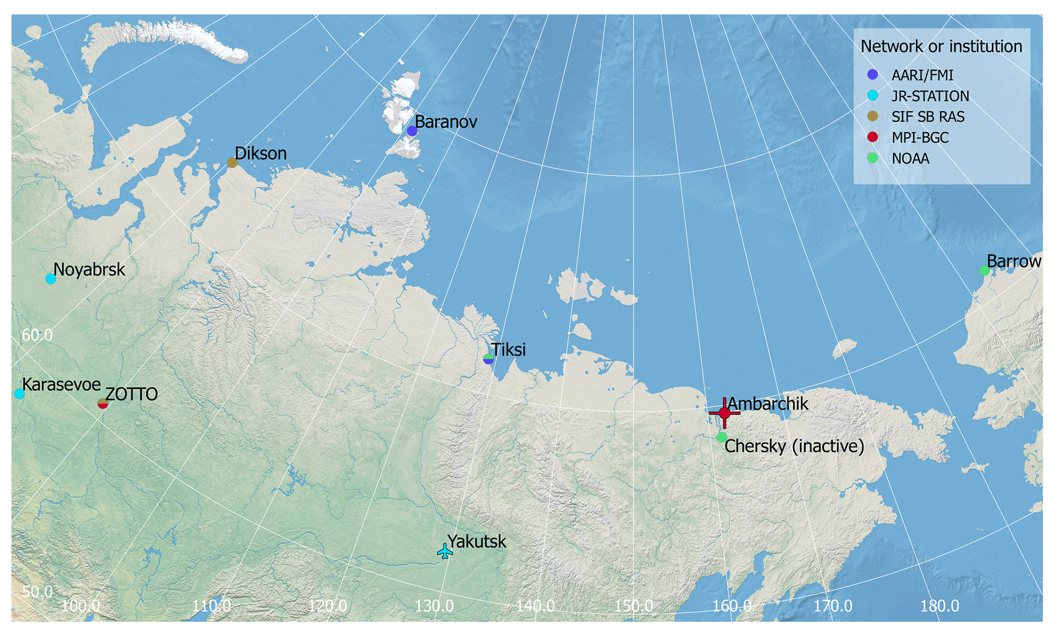
Figure 1Stations observing atmospheric CO2 and CH4 in northeastern Siberia (including Barrow, Alaska). At all stations but Yakutsk, continuous in situ monitoring takes place. At Yakutsk, flasks are sampled monthly onboard an aircraft. At Tiksi and Barrow, flasks are sampled by NOAA in addition to the continuous in situ measurements.
2.1 Area overview
Ambarchik is located at the mouth of the Kolyma River, which opens to the East Siberian Sea (69.62∘ N, 162.30∘ E; Fig. 2). The majority of the landscape in the immediate vicinity of the locality is wet tussock tundra. At the ecoregion scale, Ambarchik is bordered by Northeast Siberian Coastal Tundra ecoregion in the west, the Chukchi Peninsula Tundra ecoregion in the east, and the Northeast Siberian Taiga ecoregion in the south (ecoregion definitions from Olson et al., 2001). Major components contributing to the net carbon exchange processes in the area are tundra landscapes including wetlands and lakes, as well as the Kolyma River and the East Siberian Arctic Shelf.

Figure 2Ambarchik station location. Background based on Copernicus Sentinel data from 2016.
2.2 Site overview
Ambarchik hosts a weather station operated by the Russian meteorological service (Roshydromet), whose staff is the entire permanent population of the locality. The closest town is Chersky (∼100 km to the south, with a population of 2857 as of 2010), with no other larger permanent settlement closer than 240 km. Thus, the site does not have any major sources of anthropogenic greenhouse gas emissions in the nearby. The only regular anthropogenic CO2 and potential CH4 sources that may influence the measurements are from the Roshydromet facility, including the building that hosts the power generator and the inhabited building.
The atmospheric carbon observation station Ambarchik began operation in August 2014. It consists of a 27 m tall tower with two air inlets and meteorological measurements, while the majority of the instrumentation is hosted in a rack inside a building. The rack is equipped for temperature control, but due to the risk of overheating, it is open most of the time and thus in equilibrium with room temperature (room and rack temperature are monitored). Atmospheric mole fractions of CH4, CO2, and H2O are measured by an analyzer based on the cavity ring-down spectroscopy (CRDS) technique (G2301, Picarro Inc.), which is calibrated against WMO-traceable reference gases at regular intervals (Sect. 3.2). The tower is located 260 m from the shoreline, with a base elevation of 20 m a.s.l. (estimated based on GEBCO_2014 (Weatherall et al., 2015), which in this region is based on GMTED2010; Danielson and Gesch, 2011).
2.3 Gas handling
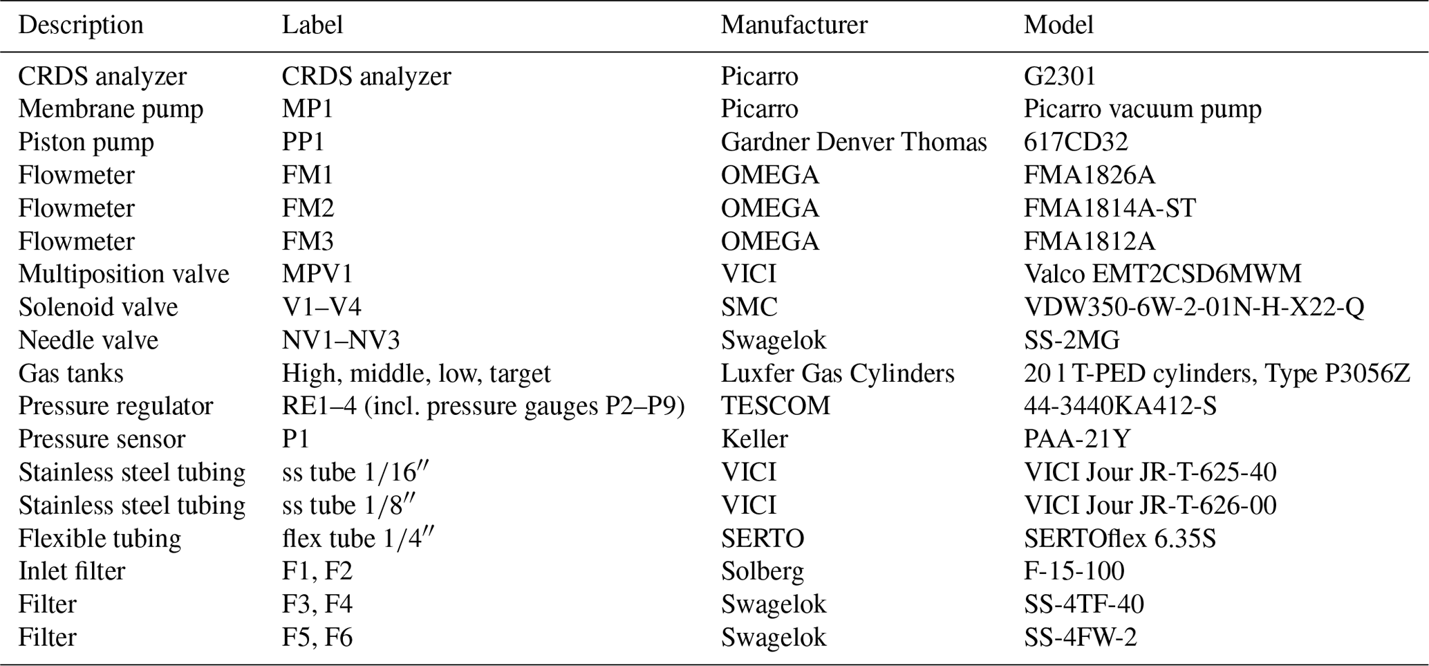
The measurement system allows for switching between two different air inlets and four different calibration gas tanks (Fig. 3). Component manufacturers and models of the individual components are listed in Table A1.
Air inlets with rain guards are mounted on the tower at 27 (“top”) and 14 (“center”) m a.g.l., respectively, and are equipped with 5 µm polyester filters (labels F1 and F2 in Fig. 3). The two air inlets are probed in turns (15 min top; 5 min center). Signals from the center inlet are mainly used for quality control purposes (Sect. 3.4). Air is drawn from the inlets (I1, I2) through lines of flexible tubing (6.35 mm outer diameter) by a piston pump located downstream of the measurement line branch (PP1). The cycles of the pump are smoothed by a buffer with a volume of about 5 L. The combined flow through both inlet lines is about 17 L min−1, monitored by a flowmeter (FM1) and limited by a needle valve (NV1). The tubing enters the house at a distance of about 15 m from the tower. The air passes 40 µm stainless steel filters (F3, F4), behind which the sample line is branched from the high flow line. A solenoid valve (V1) is used to select between the two inlets.
The sample line (between filters F3/F4 and the CRDS analyzer) is composed exclusively of components made of stainless steel; they include tubing (ss tube ), two 2 µm filters (F5, F6), a needle valve for sample flow regulation (NV2, usually fully open), a pressure sensor (P1), and a flowmeter (FM2). Air is drawn from the high flow line into the sample line by a membrane pump downstream of the CRDS analyzer (MP1). The nominal flow rate in the sample line is 170 mL min−1. The residence time of sample air in the tubing between inlets and CRDS analyzer is on the order of 12 s.
Calibration gases also pass through a line composed exclusively of stainless steel components. Air from gas tanks (“high”, “middle”, “low”, and “target”) passes through pressure regulators (RE1–4), reducing their pressure to roughly ambient pressure. This way, the CRDS analyzer can cope with the pressure difference between sample air and calibration air from the tanks without an open split, which would normally be installed to equilibrate the line with ambient pressure. This setup was chosen in order to conserve calibration air. The lines from the gas tanks are connected to a multiposition valve (MPV1), which is used to select between gas tanks. Downstream of the multiposition valve, the calibration gas line is connected to the sample line by a solenoid valve (V3). The solenoid valves V2 and V3 are used to select between sample air from the tower and calibration air.
During calibrations, the part of the measurement line that is not part of the calibration line is continuously flushed by the high flow pump (PP1) through the purge line, which comprises solenoid valve V4 (which shuts off air flow from the gas tanks through the purge line in case of a power outage during a tank measurement), needle valve NV3 (which is used to match the purge flow to the usual sample flow), and flowmeter FM3 (which monitors the purge flow).
The flowmeters (FM1–3) and pressure sensor (P1) are used to diagnose problems such as weakening pump performance, clogged filters, leaks, or obstructions.
The gas handling system was tested for leaks after installation. This was done by capping the tubing and evacuating it using a hand pump to pressures of 0.3–0.4 bar (normal operating pressure is around 0.7 bar). The leak rate was then computed from the pressure increase over several hours, corrected for temperature fluctuations measured in the lab. To mitigate the effect of inhomogeneous temperature fluctuations throughout the tubing and increase sensitivity of the pressure to small leaks, the experiments were limited to the small tubing volume inside the laboratory, ignoring the tubing on the tower. This is the part that is most susceptible to leaks, due to the number of tubing connections and the potentially higher CO2 mole fractions. The results of several such experiments indicated leak rates on the order of no more than mbar L s−1. At this rate, CO2 and CH4 contamination is negligible even with extremely high mole fractions in the laboratory. During later maintenance visits, simpler leak tests, which did not require opening tubing connections, were performed by breathing on individual connectors and observing the CO2 mole fraction measured by the gas analyzer. No indications of leaks were observed during these tests.
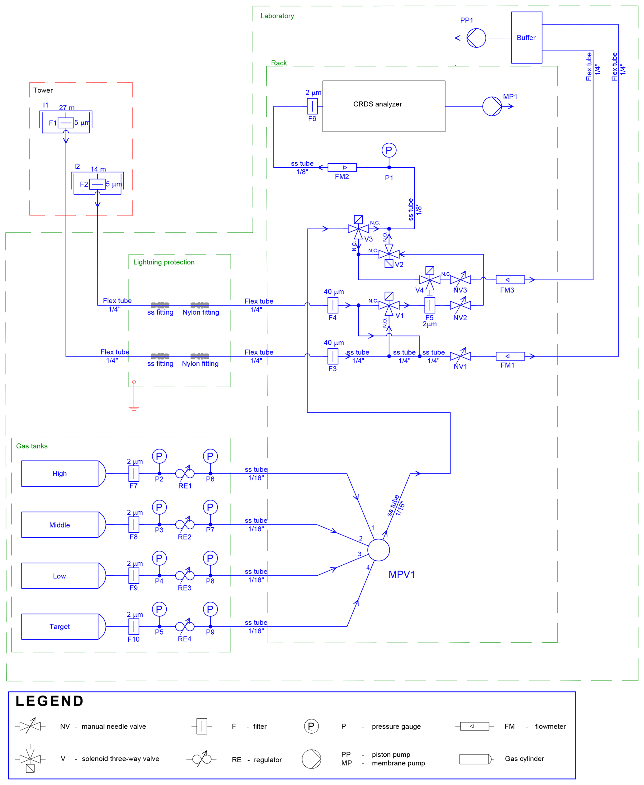
Figure 3Air flow diagram of Ambarchik greenhouse gas measurement system. See Sect. 2.3 for a description of component abbreviations. “ss” refers to stainless steel throughout the diagram.
2.4 Meteorological measurements
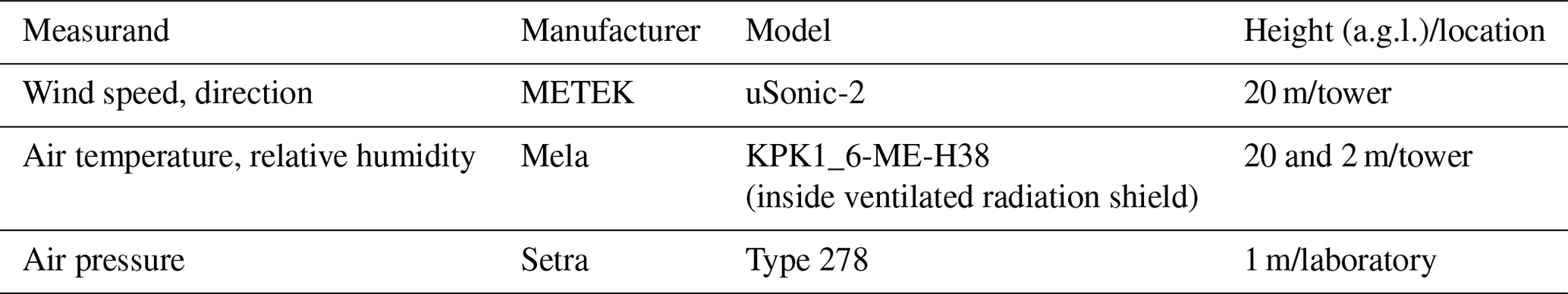
Meteorological measurements performed by the Max Planck Institute for Biogeochemistry (MPI-BGC) at Ambarchik include wind speed and direction at 20 m a.g.l., air temperature and humidity at 20 and 2 m a.g.l., and air pressure at 1 m a.g.l. (instruments listed in Table A2). The measurements mainly serve to monitor atmospheric conditions like wind and stability of atmospheric stratification for quality control of the GHG data (described in Sect. 3.4). The 2-D sonic anemometer, which is used to measure wind speed and direction, features a built-in heating to prevent freezing. The heating is switched on if the temperature decreases below 4.5 ∘C and relative humidity is higher than 85 %, and switched off when temperatures increase above 5.5 ∘C.
2.5 Power supply
Power is supplied by the diesel generator of the Roshydromet meteorological station. Power consumption of the MPI-BGC measurement system is about 350 W, and an additional 125 W is required when the heating of the sonic anemometer is switched on. In order to avoid loss of power during routine generator maintenance, an uninterruptible power supply (9130 UPS, Eaton) was installed, which is able to buffer power outages of up to about 40 min (the heating of the sonic anemometer is not powered by the UPS). In the case of a longer power loss, the UPS initiates a controlled shutdown of the CRDS analyzer.
2.6 Data logging
Trace gas measurements and related data are logged by the factory-installed software of the CRDS analyzer. All other measurements are logged by an external data logger (CR3000, Campbell Scientific). The logger samples all variables every 10 s. Raw samples are stored for wind measurements as well as flow and pressure in the tubing (FM1–FM3, P1). Of the remaining meteorological measurements, room and rack temperature, and diagnostic variables, 10 min averages are stored. The data are transferred from the external data logger to the hard drive of the CRDS analyzer daily. All data are backed up to an external hard drive hourly. The internal clocks of the CRDS analyzer and the data logger are synchronized with a GPS receiver (GPS 16X-HVS, Garmin) once per day.
3.1 Water correction
In order to minimize maintenance efforts and reduce the number of components prone to failure, CO2 and CH4 mole fractions are measured in humid air. Hence, the values reported by the analyzer have to be corrected for the effects of water vapor to obtain dry air mole fractions. This is done by applying a water correction function to the raw data:
Here, cwet is the mole fraction of CO2 or CH4 in humid air reported by the analyzer, h is the water vapor mole fraction (also measured by the CRDS analyzer), fc(h) is the water correction function, and cdry is the desired dry air mole fraction. Picarro Inc. provides a factory water correction based on Chen et al. (2010), but to achieve accuracies within the WMO goals for water vapor mole fractions above 1 % H2O, custom coefficients must be obtained for each analyzer (Rella et al., 2013). Here, we employ the novel water correction method by Reum et al. (2019). In Reum et al. (2019), data from gas washing bottle experiments (explained in Appendix B) with the CRDS analyzer in Ambarchik were analyzed in the context of the new method (labeled “Picarro no. 5” therein). Here, we use these data and data from additional experiments to derive water correction coefficients for application to the complete Ambarchik record. The results of this procedure are briefly summarized here, and more details are given in Appendix B.
Water correction experiments were performed in 2014, 2015, and 2017. Differences between the water corrections based on the different experiments were on the order of magnitude of the WMO goals (Fig. 4). Here, we chose the WMO internal reproducibility goals as a reference, which correspond to half of the interlaboratory compatibility goals (WMO, 2016). The motivation for this choice is that keeping biases of observations with respect to the calibration scale within these goals ensures that biases between stations are within the interlaboratory compatibility goals. Given the small number of water correction experiments conducted so far, it is unknown whether these differences represent drifts over long timescales, short-term variations, and/or systematic differences between the experimental methods. Stavert et al. (2019) found that variability among weekly water correction tests over 3 months was similar to that of annual tests over 2 years. This indicates that the differences of the Ambarchik analyzer could be short-term variations. In the absence of evidence for trends, water correction coefficients were derived based on the averages of the individual water correction function responses for each species (see Appendix B). The maximum deviations of the individual functions to these synthesis functions were 0.018 % CO2 at 3 % H2O, which corresponds to 0.07 ppm at 400 ppm dry air mole fraction, and 0.034 % CH4 at 2.7 % H2O, which corresponds to 0.7 ppb at 2000 ppb dry air mole fraction (Fig. 4).
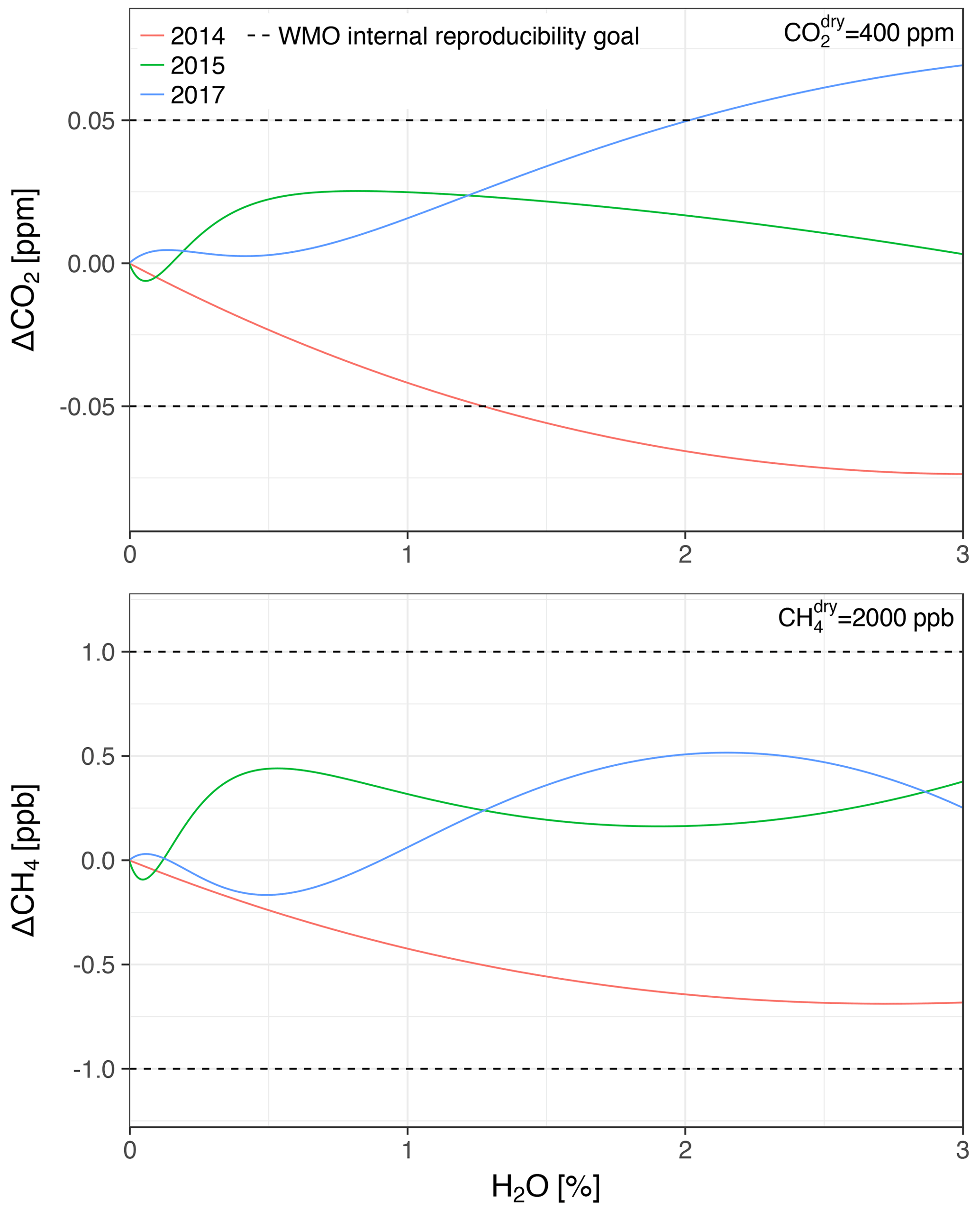
Figure 4Differences between individual water correction functions and the synthesis water correction function at dry air mole fractions of 400 ppm CO2 and 2000 ppb CH4. The dashed lines correspond to the WMO internal reproducibility goals, in the case of CO2 in the Northern Hemisphere (WMO, 2016).
3.2 Calibration
Calibrations are performed with a set of pressurized dry air tanks filled at the Max Planck Institute for Biogeochemistry (Jena, Germany). The levels of GHG mole fractions of these tanks have been traced to the WMO scales X2007 for CO2 and X2004A for CH4 (Table C1). Three calibration tanks (in order high, middle, and low) are probed once every 116 h for 15, 10, and 10 min, respectively. The longer probing time of the first (high) tank serves to flush out residual water vapor due to water molecules that adhere to the inner tubing walls. Thus, residual water vapor during tank measurements is well below 0.01 % H2O. From these three tanks, coefficients for linear calibration functions are derived. Due to the scatter of the coefficients over time, the coefficients are smoothed using a tricubic kernel with a width of 120 d (Fig. C1). Individual measurements are calibrated by applying the smoothed coefficients, interpolated linearly in time. The impact of the smoothing on the calibration of ambient mole fractions is smaller than 0.02 ppm CO2 and 0.3 ppb CH4 (1 standard deviation). The fourth tank (target) is probed every 29 h for 15 min. Its calibrated CO2 and CH4 mole fraction measurements (Fig. 5) serve as quality control of the calibration procedure (Sect. 3.3). Uncertainties associated with the calibration procedure, as well as possible future improvements, are discussed and quantified in Appendix E.
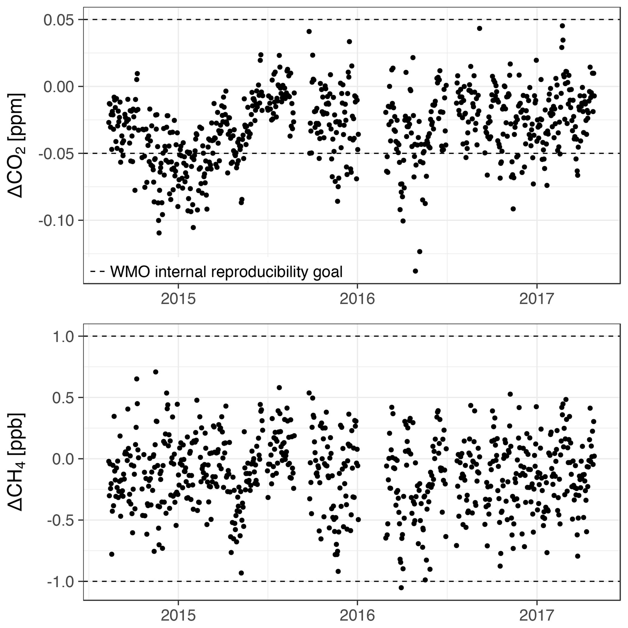
Figure 5Target tank bias over time for CO2 and CH4. As in Fig. 4, the dashed lines correspond to the WMO internal reproducibility goals.
3.3 Uncertainty in CO2 and CH4 measurements
Measurement uncertainties in the CO2 and CH4 data arise from instrument precision, the calibration, and the water correction. We estimated time-varying uncertainties of hourly trace gas mole fraction averages based on the method by Andrews et al. (2014), with some modifications. Details of the procedure are given in Appendix E.
Average uncertainties at the 1σ level were 0.085 ppm CO2 and 0.77 ppb CH4. Both were dominated by the variability between the water vapor correction experiments. The contribution of analyzer signal precision for averages over 1 h to these uncertainties was 0.013 ppm CO2 and 0.25 ppb CH4. These numbers may be used to distinguish analyzer signal precision from atmospheric variability.
3.4 Data screening
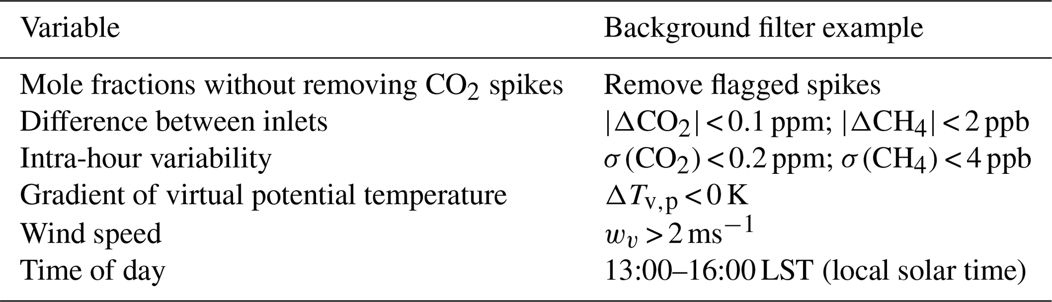
After water correction and calibration, invalid data are automatically removed before calculating hourly averages using filters for bad analyzer status (Sect. 3.4.1), flushing of lines (Sect. 3.4.2), times of calibration and maintenance, contamination from local polluters (Sect. 3.4.3), and water vapor spikes (Sect. 3.4.4). In the case of contamination from local polluters, CO2 and CH4 averages are also computed with the flagged data to allow for assessment of the impact of the filter. Additional variables reported in the hourly averages allow for further data screening, e.g., for using the data in inverse models (Table 1). Details on the gradient of virtual potential temperature are given in Sect. 3.4.5.
Table 1Variables for data screening and an example of a strict filter for background conditions that was used to infer average growth rates in Sect. 5.1.
3.4.1 Analyzer status diagnostics
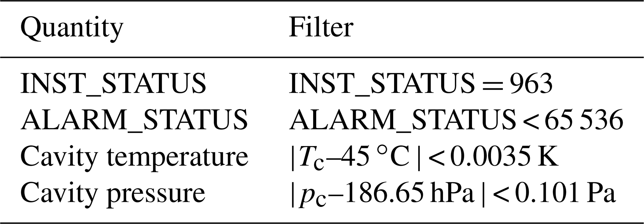
Picarro Inc. provides the diagnostic flags INST_STATUS and ALARM_STATUS that monitor the operation status of the analyzer. The values in Table 2 indicate normal operation. The flag ALARM_STATUS indicates both exceeding user-defined thresholds for high mole fractions (ignored here), and data flagged as bad by the data acquisition software. The code reported in INST_STATUS contains, among other indicators, thresholds for cavity temperature and pressure deviations from their target values. We created stricter filters for these two values based on their typical variation during normal operation of this particular measurement system. Occasionally, small numbers (< 5) of outliers are recorded after a period of lost data (e.g., due to high CPU load). These are removed manually.
Table 2Diagnostic values indicating normal status of the CRDS analyzer.
3.4.2 Flushing of measurement lines
Air from the two inlets at the tower and the calibration tanks flows through some common tubing (Fig. 3). Hence, air measured immediately after a switch is influenced by the previous air source. We remove the first 30 s from the record after a switch between inlets to avoid sample cross-contamination. Air from calibration tanks exhibits larger differences in humidity and mole fractions to ambient air. Hence, the first 5 min of ambient air measurements after tank measurements are removed from the record.
3.4.3 Contamination from local polluters
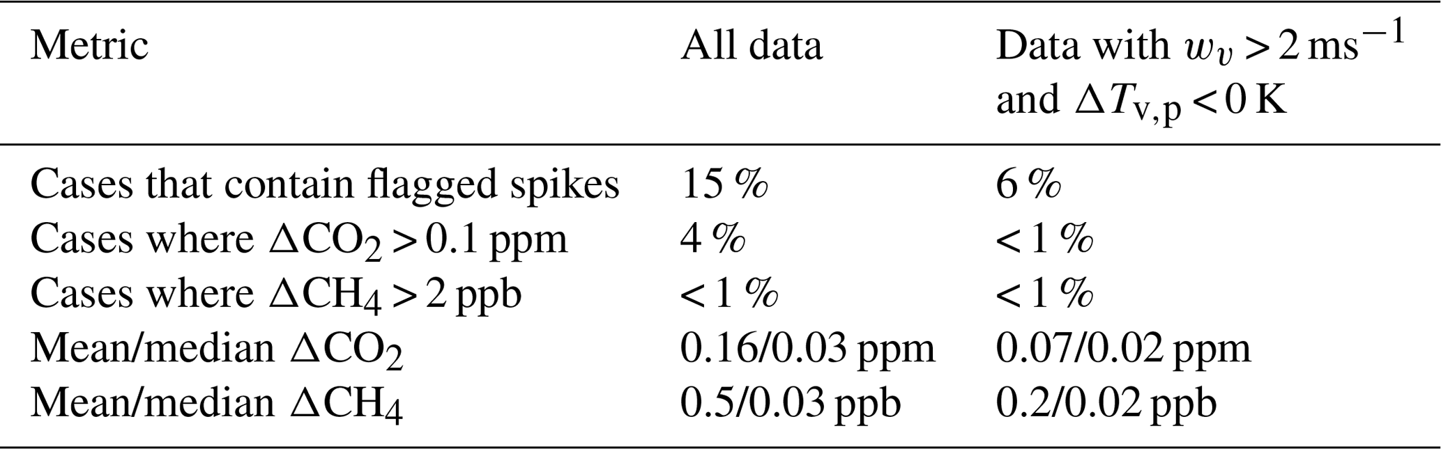
Possible frequent contamination sources in the immediate vicinity of the tower are the building hosting the power generator of the facility (65 m northwest of the tower), the heating and oven chimneys of the only inhabited building (30 and 20 m northeast, respectively), and waste disposal. These local polluters can cause sharp and short increases in CO2 and CH4 mole fractions on the timescale of seconds to a few minutes. These features cannot be modeled by a regional or global atmospheric transport model and should therefore be filtered out. We developed a detection algorithm to identify spikes based on their duration, gradients, and amplitude in the raw CO2 data. Spike detection algorithms are often compared to manual flagging by station operators (El Yazidi et al., 2018). Parameters of our algorithm were tuned in this way based on the first year of data. The algorithm is described in Appendix D. The impact of the CO2 spike flagging procedure is shown in Table 3. Impacts on the hourly mole fractions are small, more so when considering only data that pass other quality filters.
We observed that large CH4 spikes were much less frequent than and often coincided with CO2 spikes. Hence, the spike detection algorithm developed for CO2 was used to flag CH4 as well. This strategy may remove some unpolluted CH4 signals and, in rare cases, leave contaminated CH4 signals undetected. However, given the small impact of filtering flagged CO2 spikes and the smaller frequency of large CH4 spikes, we think that contamination of CH4 independent of CO2 is a negligible source of error in Ambarchik data. Furthermore, due to the large variability of natural CH4 sources, a spike detection algorithm for CH4 may bear the risk of flagging natural signals. In addition, contamination of CH4 data may also be flagged based on other criteria, in particular their intra-hour variability. For these reasons, we decided that a common filter for both CO2 and CH4 works best at Ambarchik.
Table 3Fraction of hourly averages of all data from the top inlet that contain flagged CO2 spikes, and impact of removing them before averaging (ΔCO2, ΔCH4).
3.4.4 Water vapor spikes
During winter, the CRDS analyzer occasionally records H2O spikes with durations of a few seconds. The spikes typically exhibit much higher mole fractions than possible given ambient air temperature. This suggests that they are caused by small amounts of liquid water in the sampling lines in the laboratory upon evaporation. As we observed the phenomenon exclusively during the cold season, we speculate that it is caused by small ice crystals that may form on the air inlet filters (F1, F2), detach, are trapped by one of the filters inside the laboratory, and evaporate.
Due to the fact that fast water vapor variations deteriorate the accuracy of the water vapor correction, we remove the spikes before creating hourly averages. Spikes are identified using a flagging procedure similar to the one for CO2 contamination described in Appendix D, with parameters adapted to the different shape of the H2O spikes.
3.4.5 Virtual potential temperature
Regional- and global-scale atmospheric tracer transport models rely on the assumption that the boundary layer is well-mixed (e.g., Lin et al., 2003). This requirement is not satisfied when the air is stably stratified due to a lack of turbulent mixing (Stull, 1988). This may occur when the virtual potential temperature increases with height. To detect these situations, sensors for temperature and relative humidity are installed at 2 and 20 m above ground level on the measurement tower (Table A2). Based on these measurements, the virtual potential temperature is calculated for both heights, and the difference can be used as an indicator for stable stratification of the atmospheric boundary layer at the station (e.g., Table 1 and Sect. 5.1).
The predominant wind directions at Ambarchik were southwest and northeast (Fig. 6) over the analyzed period (August 2014–April 2017). Southwesterly winds dominated from October to March, while northeasterly winds dominated from April to August. September and October were a transitional period.
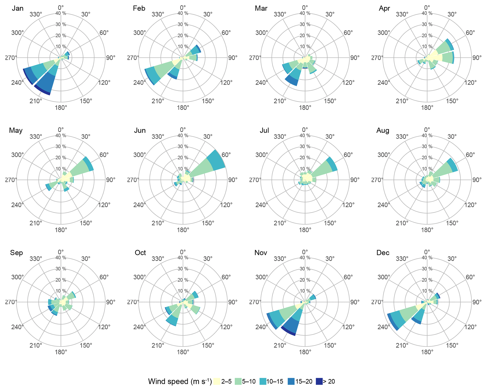
Figure 6Wind distribution at Ambarchik for wind speeds > 2 ms−1 for the period from August 2014 to April 2017.
We used an atmospheric transport model (Henderson et al., 2015) to determine regions within the Arctic that influence the atmospheric signals captured at Ambarchik. For the case studies shown here, 15 d back trajectories were calculated for the period from August 2014 to December 2015. Atmospheric transport was modeled using STILT (Lin et al., 2003) driven by WRF (Skamarock et al., 2008), for which boundary and initial conditions were taken from MERRA reanalysis fields (Rienecker et al., 2011). The resolution of the transport model in our domain was mostly 10 km horizontally with 41 vertical levels. Based on these trajectories, the sensor source weight functions (“footprints”) were calculated on a square-shaped Lambert azimuthal equal area grid with a resolution of 32 km and an extent of 3200 km centered on Ambarchik. To better visualize the representativeness of Ambarchik data to different origins of air masses, we aggregated these footprints over seasons. Furthermore, we sorted the aggregated footprints into bins each covering a quartile of the cumulative footprint (Fig. 7). Footprints covered adjacent northeast Siberian tundra and taiga ecoregions as well as the East Siberian Arctic Shelf, with seasonally varying influences. In winter, spring, and summer, the top quartile of the footprint concentrated on a few grid cells (order of ∼100 km) around Ambarchik, with a slightly larger spread in fall. The two central quartiles had a focus on easterly directions in spring and on the north in summer.
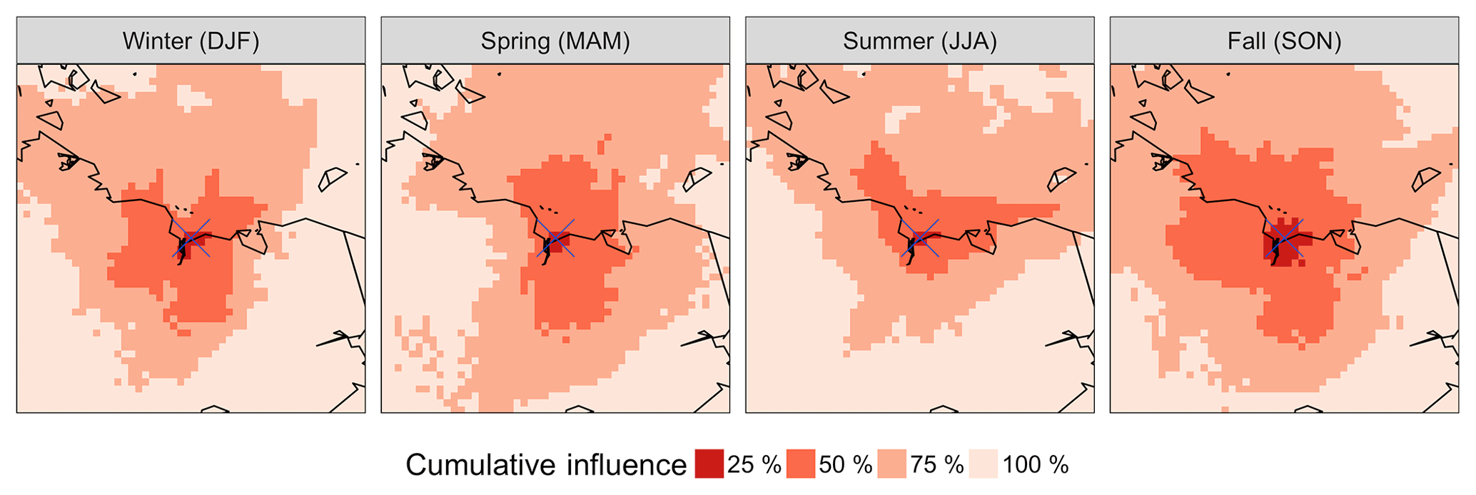
Figure 7Cumulative Ambarchik footprints based on 15 d back trajectories for August 2014–December 2015. The footprints were aggregated over the winter (December–January–February), spring (March–April–May), summer (June–July–August), and fall (September–October–November) seasons, and sorted into bins covering 25 % of the cumulative influence each. Shown here is a zoom in of the center of the 3200 km × 3200 km domain on which the footprints were computed, covering 1600 km × 1600 km.
5.1 Ambarchik time series in comparison with Barrow, Alaska
In order to provide a context for the characteristics of greenhouse gas signals measured at Ambarchik, we compared the time series from Ambarchik with in situ CO2 (NOAA, 2015) and CH4 (Dlugokencky et al., 2017) mole fractions observed at Barrow Observatory, Alaska, which is located close to the village of Utqiaġvik (71.32∘ N, 156.61∘ W). Data from Barrow were chosen for the comparison because of the station's proximity to Ambarchik (distance ∼1500 km, latitudinal difference 1.7∘; cf. Fig. 1), and because they have been used in many studies on both global and regional greenhouse gas fluxes (e.g., Berchet et al., 2016; Jeong et al., 2018; Rödenbeck, 2005; Sweeney et al., 2016). The analyzed period was August 2014 to December 2016.
For the comparison, afternoon data (13:00–16:00 LST) for which the wind speed was above 2 ms−1 were used (gaps in the MPI-BGC wind measurements were filled with Roshydromet 10 m wind speed data). In addition, Ambarchik data were filtered out when the virtual potential temperature increased with height. This filter was omitted for Barrow, because it would have removed most of the data from October to April, including data classified as “background” signals (which occurred throughout the year). Barrow data were filtered according to their three-character quality flag. For CO2, data with quality flags “…”, “.D.”, “.V.”, and “.S.” were included. For CH4, data with quality flags “…” and “.C.” were included. Data with flags beginning with a character other than a “.” in the first column were removed as invalid. Quality flags differing with respect to the second or third character from those listed above were excluded, as their number was negligible. We inferred average growth rates and seasonal cycles for the analyzed period based on the curve fitting procedure by Thoning et al. (1989): linear trends and four harmonics representing the seasonal cycles were fitted to the data, and a low-pass filter was applied to the residuals. We emphasize that the purpose of this procedure was not to infer baselines, which would not be suitable for CH4. Instead, the fitted curves were smooth representations of the time series, including regional signals. To minimize the influence of interannual variations on the estimated average growth rates at Ambarchik, they were estimated with additional strict filters for background conditions applied to Ambarchik data (Table 1). Given the short duration of the Ambarchik record, we estimated seasonal cycle amplitude and timing based on the harmonic part of the fit function, which was more robust than including smoothed residuals.
5.1.1 Carbon dioxide
In spring, CO2 mole fractions observed at Ambarchik closely tracked those measured at Barrow (Fig. 8), which was likely due to the absence of local to regional sources and sinks during this period. In summer, Ambarchik recorded a stronger seasonal drawdown of CO2 mole fractions compared with Barrow, leading to a lower minimum value that occurred 12 d earlier. In fall, CO2 rose faster at Ambarchik, reaching the midpoint between minimum and maximum 21 d earlier than Barrow. The mole fraction maxima in winter were at similar values. Carbon dioxide mole fractions at Ambarchik were more variable than at Barrow in summer and fall, which indicates stronger local and regional sources and sinks captured by the Ambarchik tower. The annual amplitude of CO2 was slightly larger at Ambarchik (20 ppm vs. 18 ppm) because of the lower summer minimum. The average growth rates were (2.77±0.09) and (2.82±0.05) ppm CO2 yr−1 at Ambarchik and Barrow, respectively. Note that despite the good agreement of these growth rates, their uncertainties are larger than the statistical uncertainties given here, as the estimates depended on data selection and were based on less than 3 years of data. We note that in November and December 2016, exceptionally high CO2 mole fractions were measured at Ambarchik. However, analysis of individual signals is beyond the scope of this paper.
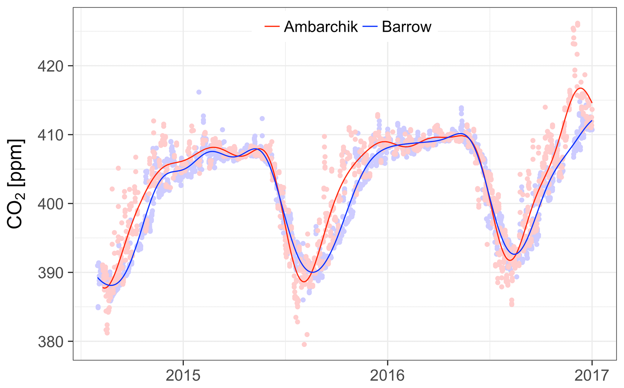
Figure 8Atmospheric CO2 and CH4 measurements from Ambarchik and Barrow. Points are quality-controlled hourly averages; lines are the results of a curve fit plus smoothed residuals (see text for details).

5.1.2 Methane
Similar to CO2 mole fractions, in spring, CH4 mole fractions at Ambarchik matched those at Barrow and had low variability (Fig. 8). Throughout the rest of the year, CH4 mole fractions at Ambarchik were higher and more variable than at Barrow, which is reflected by the larger annual amplitude of 72 ppb at Ambarchik, compared with 47 ppb at Barrow. The summer minimum of the harmonics occurred 70 d earlier at Ambarchik. By contrast, the minimum of the visual baseline of hourly data occurred much later, and was close in values and timing to the Barrow measurements (Fig. 9). This discrepancy was due to the fact that the harmonics fitted to Ambarchik CH4 data were influenced by large positive CH4 enhancements starting in early summer, which were likely caused by strong regional sources. Such CH4 enhancement events were also recorded throughout most of the winters. Estimated average growth rates of CH4 were 6.4±1.0 ppb yr−1 at Ambarchik and 10.0±0.7 ppb yr−1 at Barrow. Note that, as for CO2, the true uncertainties of these growth rates are larger than the statistical uncertainties given here, as the estimates depended on the data selection.
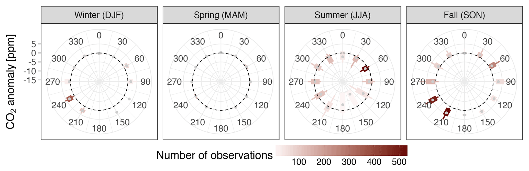
Figure 10Carbon dioxide anomalies plotted against wind direction. The dashed circle is the baseline (anomaly 0 ppm). The (gray) points are the median, boxes the first and third quartile, and whiskers the first and ninth decile. Shown here are data that passed the filters for low wind speeds and temperature inversions (Table 1). The color of boxes and whiskers indicates the number of measurements available in each bin.
5.2 Angular distribution of regional CO2 and CH4 anomalies
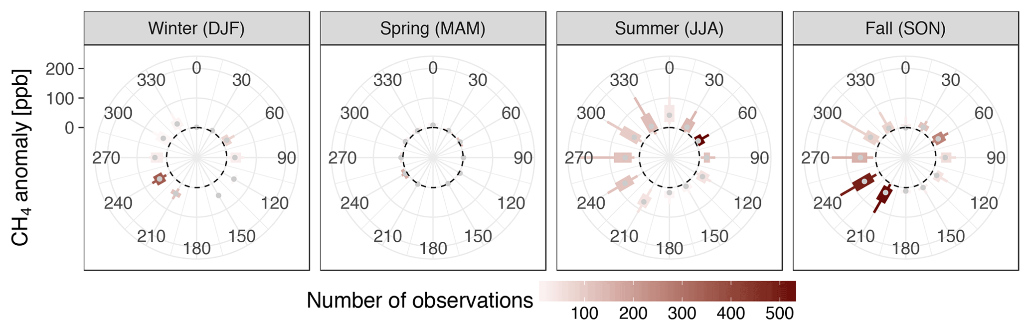
Ambarchik is located at a junction of several different ecoregions, and in particular at the coast of the East Siberian Sea. Therefore, the dependence of CO2 and CH4 signals on wind direction could provide insights into CO2 and CH4 exchange between these different regions and the atmosphere. We examined this dependence based on CO2 and CH4 anomalies representative of fluxes inside the domain introduced in Sect. 4 (3200 km × 3200 km, centered on Ambarchik). These anomalies were computed following a standard method in regional inverse modeling of atmospheric tracer transport, i.e., by subtracting the contribution of CO2 and CH4 transported into the domain (the background signal) from the observations. Therefore, the anomalies represent the atmospheric signature of sources and sinks inside the domain. The background signal was computed by sampling global atmospheric CO2 and CH4 mole fraction fields at the end points of the back trajectories introduced in Sect. 4. The global CO2 fields were based on Rödenbeck (2005, version https://doi.org/10.17871/CarboScope-s04_v3.8.), and the CH4 fields were based on the code by Rödenbeck (2005) modified by Tonatiuh Guillermo Nuñez Ramirez (personal communication, 2018). Both fields were optimized for station sets that included Ambarchik data. We analyzed the data that passed the filters for low wind speeds and temperature inversions (see Table 1) grouped by season, and focused the interpretation on the signals from the predominant wind directions, as sample sizes from other sectors were small.
5.2.1 Carbon dioxide
The most pronounced CO2 signals from predominant wind directions were positive anomalies during southwesterly winds in fall and winter. During summer, CO2 anomalies from the predominant wind direction (northeast) were small. During spring, almost no CO2 anomalies were observed.
5.2.2 Methane
The strongest CH4 enhancements were observed from westerly winds in summer, and southwesterly winds in fall and winter. The predominant northeasterly winds in summer carried comparatively small CH4 enhancements. The overall variability of CH4 was highest in summer and fall, with considerable enhancements especially from the southwest in winter. Like CO2, CH4 showed almost no anomalies in spring.
In this paper, we presented the first years (August 2014–April 2017) of CO2 and CH4 measurements from the coastal site of Ambarchik in northeastern Siberia. The site has been operational without major downtime since its installation. Greenhouse gas measurements are calibrated about every 5 days using dry air from gas tanks with GHG mole fractions traced to WMO scales. Mole fractions of CO2 and CH4 are measured in humid air and corrected for the effects of water vapor using a novel water vapor correction method. An algorithm was developed to remove measurements influenced by local polluters, which affected a small fraction of the measurements. Measurements of the gradient of the virtual potential temperature and the two sampling heights allow for detection of stable stratifications of the atmospheric boundary layer at the station. Uncertainties of the GHG measurements, which were inferred from measurements of dry air from calibrated gas tanks and water correction experiments, were 0.085 ppm CO2 and 0.77 ppb CH4 on average. We continue work on improvements of the accuracy of the calibrations and uncertainty estimates and will adapt them as additional information becomes available (e.g., based on post-deployment calibration of used gas tanks).
A footprint analysis indicates that Ambarchik is sensitive to trace gas emissions from both the East Siberian Sea and terrestrial ecosystems. Both CO2 and CH4 anomalies were large during southwesterly and westerly winds and small during northeasterly winds. This suggests that the larger signals originated from terrestrial rather than oceanic fluxes and demonstrates the value of sampling at the Ambarchik location for distinguishing fluxes from different source regions and, thus, insights into carbon cycle processes in this region. In comparison with Barrow, Alaska, Ambarchik recorded larger CO2 and CH4 anomalies, which resulted in larger seasonal cycle amplitudes as well as earlier minima and fall growth. We interpret the stronger CO2 and CH4 signals at Ambarchik as stronger local and regional fluxes compared with those captured at Barrow. Strong CH4 enhancements were recorded at Ambarchik well into the winter, which is evidence for the relevance of cold season emissions (Kittler et al., 2017b; Mastepanov et al., 2008; Zona et al., 2016). While the average growth rate of CO2 at Ambarchik matched that at Barrow, the growth rate of CH4 at Ambarchik was smaller. We attribute the discrepancy to the short analysis period, which makes the growth rate estimate sensitive to interannual variability and differences in the timing of the annual maximum and minimum.
The accuracy of the CO2 and CH4 data obtained at Ambarchik, and their sensitivity to sources and sinks of high-latitude terrestrial and oceanic ecosystems make the Ambarchik station a highly valuable tool for carbon cycle studies focusing on both terrestrial and oceanic fluxes from northeastern Siberia.
Quality-controlled hourly averages of data from Ambarchik are available upon request from Mathias Göckede. We plan to publish continuous updates to the data to an open access repository in the future. For access to data from Barrow, see NOAA (2015) and Dlugokencky et al. (2017).
The influence of water vapor on CO2 and CH4 measurements was corrected for based on several water correction experiments and a novel water correction model, which we describe in the following paragraphs. For more details, please refer to Reum et al. (2019). As stated in Sect. 3.1, data from gas washing bottle experiments (explanation below) with the CRDS analyzer located in Ambarchik were analyzed in Reum et al. (2019) in the context of the new water correction method (labeled “Picarro no. 5” therein). Here, we use these data and data from additional experiments to derive water correction coefficients for application to the complete Ambarchik record.
Experiments were performed with two different humidification methods. For the so-called droplet method, a droplet of deionized water (ca. 1 mL) was injected into the dry air stream from a pressurized air tank and measured with the CRDS analyzer. The gradual evaporation of the droplet provided varying water vapor levels. By contrast to the droplet method, the gas washing bottle method was designed to hold water content in the sampled air at stable levels. For this purpose, the air stream from a pressurized tank was humidified by directing it through a gas washing bottle filled with deionized water, resulting in an air stream saturated with water vapor. The humid air was mixed with a second, untreated air stream from the same tank. Different water vapor levels were realized by varying the relative flow through the lines using needle valves.
Table B1Synthesis water correction coefficients. Uncertainties are approximated by the maximum difference between the coefficients of the individual water correction functions and the coefficient of synthesis function.
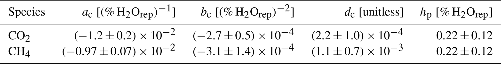
Initial experiments were performed using the droplet method, but systematic biases in the resulting dry air mole fractions at H2O < 0.5 % led to further experiments with the gas washing bottle method and the development of an improved water correction model:
Here, corrects for dilution and pressure broadening (Chen et al., 2010). The parameters dc and hp correct for a sensitivity of pressure inside the measurement cavity of Picarro analyzers to water vapor (Reum et al., 2019).
Three droplet experiments were performed in 2014, and one gas washing bottle experiment was performed in 2015 and 2017, respectively. The droplet results proved unsuitable to derive the pressure-related coefficients dc and hp due to fast variations of water vapor, which typically occurred below 0.5 % H2O (Reum et al., 2019). Therefore, from the droplet experiments only the data with slowly varying water vapor were used, and dc and hp were only based on the gas washing bottle experiments. For each species, a synthesis water correction function was derived by fitting coefficients to the average response of the individual functions (Table B1).
Table C1Calibrated dry air mole fractions of the air tanks in use at Ambarchik over the period covered in this paper. For a discussion of the uncertainties, see Appendix E2.
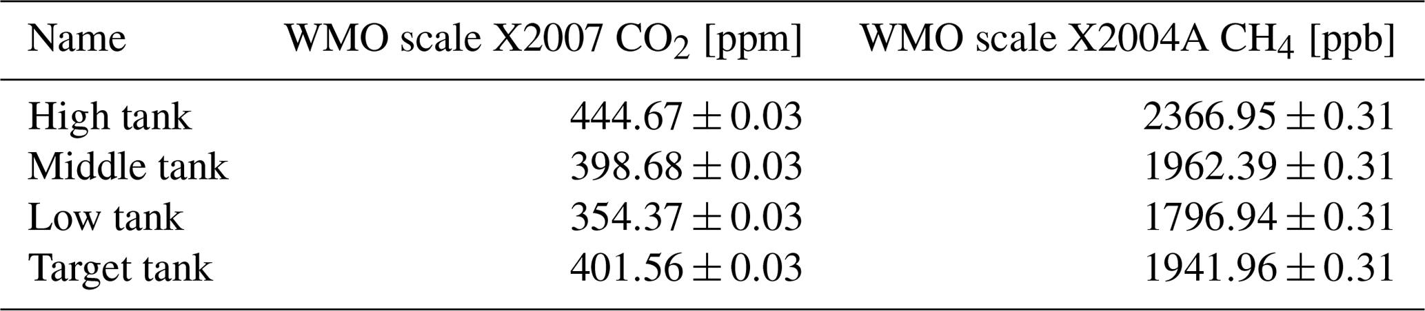
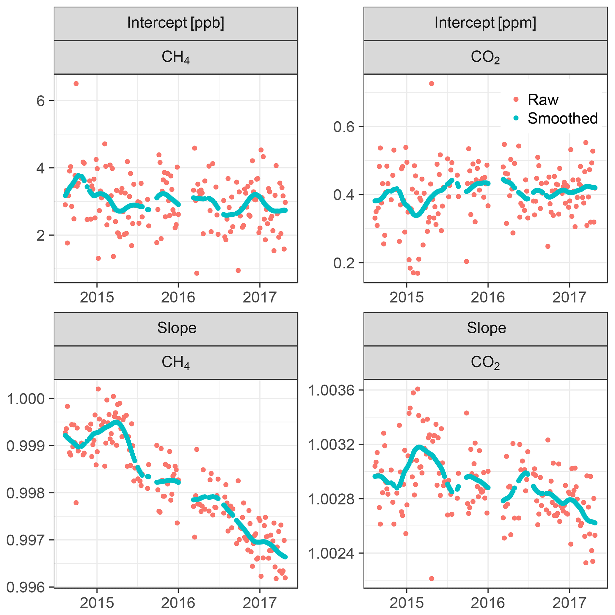
Figure C1Coefficients of linear fits to the high, middle, and low tanks. The smoothed coefficients are used for calibrating data.
The CO2 spike detection algorithm is a multistep process. First, candidates for CO2 spikes are identified. In subsequent steps, false positives are removed. Parts of the algorithm are based on Vickers and Mahrt (1997).
Step 1. Identifying spike candidates based on variation of differences between CO2 measurements
For this step, data are processed in intervals spanning 1.5 h. Candidates for CO2 spikes are identified based on the variability of differences between individual consecutive CO2 measurements. Measurements with differences that exceed 3.5 standard deviations from non-flagged data are flagged as spike candidates. As flagging the data changes the standard deviation of the non-flagged data, flagging is repeatedly applied until changes between standard deviations of the non-flagged data between the last and second-last loop are less than 10−10 ppm CO2. In some cases, this procedure flags the complete interval as spikes. This happens when the variations throughout the interval are rather uniform. This might be the case both in the presence of spikes throughout the interval, or in the absence of spikes altogether. To avoid false positives, all flags are removed, and the interval is considered to have no spikes. Cases with many spikes throughout the interval can be filtered based on the intra-hour variability flag.
Step 2. Blurring
Around the top of a spike, differences between individual CO2 soundings are often small; thus, these measurements are not captured as part of a spike in step 1. To unite the ascending and descending parts of spikes, the 20 data points before and after a flagged measurement are flagged. From here on, each group of consecutive flagged measurements is considered a spike candidate.
Step 3. Unflagging individual outliers
Step one often identifies individual or very few consecutive data points as spikes, spanning a few seconds. We regard these very small groups of flagged data points as noise misidentified as spikes. After blurring (step 2), these individual outliers form groups of at least 41 data points. In step 3, spike candidates consisting of less than 45 data points are unflagged.
Step 4. Baseline and detrending
For each spike candidate, the baseline is identified as a linear fit to the unflagged measurements within 5 min of any data point of the spike candidate. Using this baseline, the data in this interval are detrended, including the spike candidate.
Step 5. Spike height
From the detrended data from step 4, the maximum deviation from the baseline (“spike height”) is calculated. Spike candidates smaller than 8 standard deviations of the baseline measurements are unflagged.
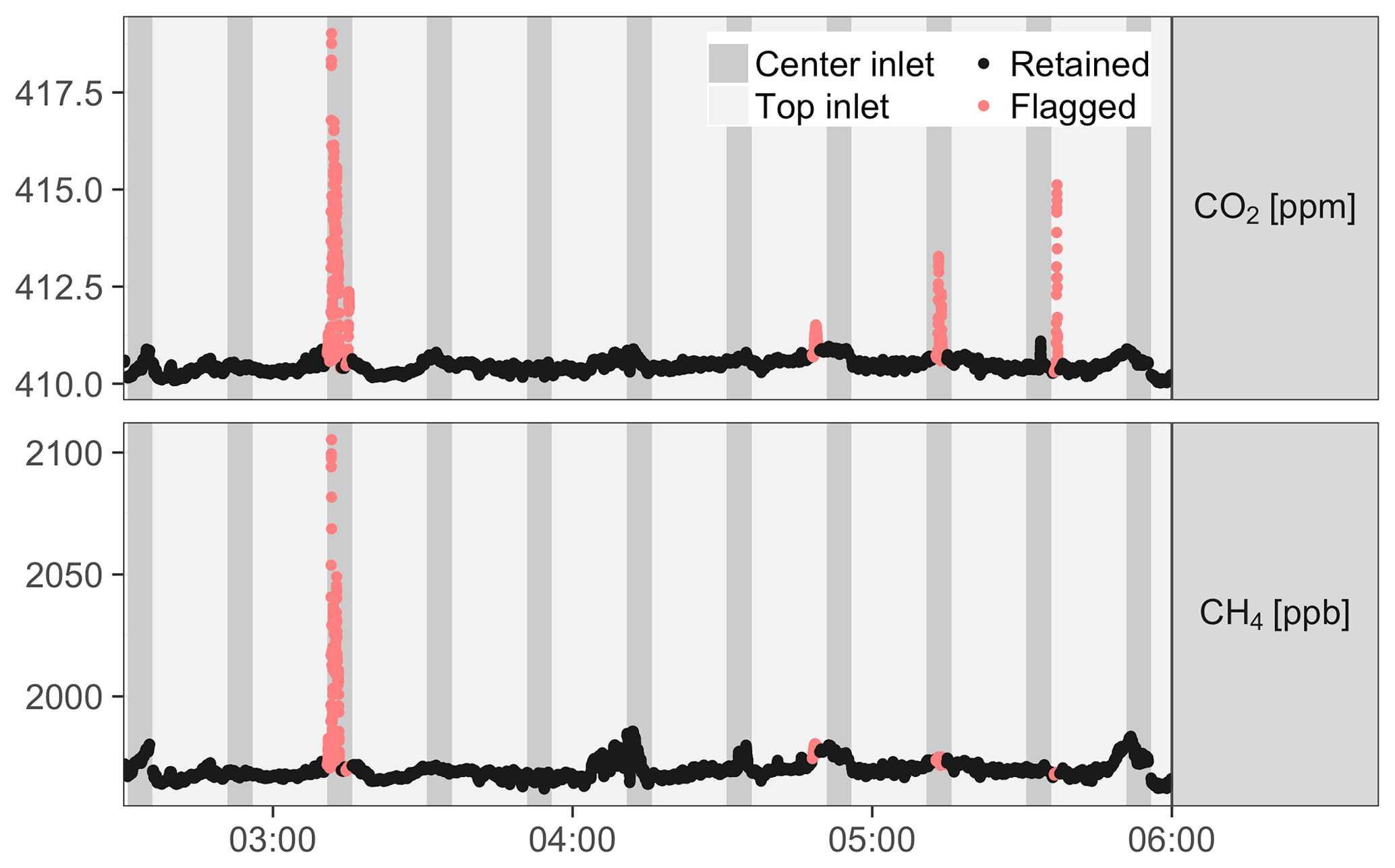
Figure D1Example of a series of flagged CO2 spikes from 4 December 2016. All times shown are UTC.
Step 6. Unflagging abrupt but persistent changes
Until the previous step, the algorithm flags abrupt CO2 changes even if they are persistent. This pattern occurs for example during changes of wind direction and does not constitute an isolated spike. In this case, a trough is present in the detrended spike. The minimum deviation from the baseline is calculated (“trough depth”) and compared to the spike height. As spike height and trough depths can be based on few data points, the influence of noise is strong. To counteract, spike height and trough depth are diminished by 2 standard deviations of the baseline. Spike candidates with trough depths greater than one-fifth of the spike height are unflagged.
Step 7. Unflagging persistent variability changes
The procedure so far can flag the beginning or end of longer periods of larger CO2 variability. To unflag these false positives, steps 4–5 are applied again with the following changes: (1) a longer baseline of 30 min before and after the spike candidate (instead of 5 min) is used, (2) baseline standard deviations are calculated separately for the period before and after the spike candidate, (3) the spike height from step 5 is used instead of recalculated, and (4) the spike height must exceed the maximum of the 2 baseline standard deviations by a factor of 6 instead of 8.
Step 8. Repeat
The result from steps 4–7 depends on unflagged data points surrounding a
spike candidate. Therefore, these steps are repeated until a steady state is
reached.
An example of flagged spikes is shown in Fig. D1.
In this example, removing flagged data reduced the hourly averages of the center
inlet data between 03:00 and 04:00 UTC by 0.5 ppm (CO2) and 7.0 ppb
(CH4). No top inlet data were flagged in this period. As small
spikes can be hard to distinguish from natural signals, some smaller
features that may be classified
as spikes upon visual inspection can pass the algorithm without being flagged, e.g., at 05:33 UTC in
Fig. D1. However, given that larger spikes alter
hourly averages by values on the order of magnitude of the WMO goals, the
impact of these features is likely negligible. In this particular example,
removing the detected spikes reduced average CO2 mole fractions between
05:00 and 06:00 UTC from the center inlet by 0.07 ppm. Removing the unflagged small
spike at 05:33 UTC would further reduce this average by 0.005 ppm, which is
inconsequential.
We adopted the uncertainty quantification method of Andrews et al. (2014). Here, we summarize the main ideas of this approach, the modifications we made, and quantify individual uncertainty components. A detailed description of the nomenclature and method was omitted; please refer to Andrews et al. (2014).
E1 Uncertainty estimation framework by Andrews et al. (2014) and modifications
Andrews et al. (2014) calculated the measurement uncertainty as the largest of four different formulations (Eq. 9a–d therein). Formulations (a) and (b) were the prediction interval of the linear regression of the calibration tanks, which takes the standard error of the fit (sefit) and the uncertainty in the analyzer signal into account. The difference between (a) and (b) was the estimate of the uncertainty in the analyzer signal. In formulation (a), this uncertainty was estimated from a model (σu) that accounts for analyzer precision (up) and drift (ub), uncertainty of the water vapor correction (uwv), equilibration after switching calibration tanks (ueq), and extrapolation beyond the range covered by the calibration tanks (uex). In measurement uncertainty formulation (b), the uncertainty estimate of the analyzer signal was estimated from the residuals of the linear fits of the calibration tank mole fractions (σy), accounting for the fact that the assigned values of the calibration tanks have non-zero uncertainty (σx):
Here, m is the slope of the calibration function. Formulation (c) was the bias of the target tank (uTGT), and formulation (d) was the uncertainty in the assigned values of the calibration tanks (σx). In this approach, uncertainty formulations (b), (c), and (d) only accounted for uncertainties of dry air measurements. Hence, we modified them by adding the uncertainty of the water correction to these formulations. Thus, the analyzer precision model for uncertainty formulation (a) became
Thus, the full uncertainty terms were as follows:
Here, z(α,f) is a factor based on the quantile function of Student's t distribution with confidence level α (α=0.675 for prediction interval at 1σ level) and degrees of freedom f. Calibration uncertainties were estimated based on the averaging strategy for coefficients, i.e., using linear fits of weighted observations from individual calibration episodes over a window of 120 d (Sect. 3.2), which usually contained about 25 calibration episodes. The standard error of the fit (sefit) was computed based on these weighted fits. In the notation of Andrews et al. (2014), the equations for sefit become (cf. Taylor, 1997):
Here, all quantities are as in Andrews et al. (2014), with the addition of weights wi and degrees of freedom f, which change with the number of calibration episodes in an interval.
Compared to calibrating based on single calibration episodes, this affected the uncertainty because of the larger number of observations (reduction of sefit and z(α,f)), and because of drift of the analyzer signal over the averaging window (increase of sefit and .
E2 Uncertainty components and estimates
In the following paragraphs, the individual components of the four uncertainty estimates Eqs. (E3)–(E6) are described. For numerical values of the components, see Table E1. The time-varying uncertainty estimates are shown in Fig. E1.
E2.1 Water vapor (uwv)
For the water correction uncertainty uwv, we used the maximum of the difference between individual water correction functions and the synthesis water correction function, i.e., 0.018 % CO2 and 0.034 % CH4, regardless of actual water content. This approach likely overestimates uwv at low water vapor content, but was chosen because uwv was not well constrained by the small number of water correction experiments conducted so far.
E2.2 Assigned values of calibration gas tanks (σx)
For the uncertainty of the assigned values of the calibration gas tanks σx, we followed the approach by Andrews et al. (2014), who set them to the reproducibility of the primary scales WMO X2007 (CO2) and WMO X2004 (CH4). Estimates based on the MPI-BGC implementations of the primary scales yielded smaller uncertainties that underestimated the mismatch between the CO2 mole fractions of the calibration tanks.
E2.3 Target tank (uTGT)
The uncertainty based on the target tank measurements uTGT was the same as in Andrews et al. (2014), but with the weighting and window we used for smoothing the calibration coefficients.
E2.4 Analyzer signal precision model (σu)
For the analyzer signal precision model σu, analyzer precision (up) and drift (ub) were estimated jointly () as the standard deviation of hourly averages of a gas tank measurement over 12 d prior to field deployment. Note that sefit also accounts for drift of the analyzer signal. However, the contribution of drift on timescales significantly shorter than the averaging window of 120 d to sefit tends toward zero. As the estimate of ub was based on 12 d of measurements, it represents drift over this shorter timescale in the prediction interval, which is why it was included in the model. The other components (σeq, σex) appeared negligible. In particular, we found no conclusive evidence of non-negligible equilibration errors (σeq) in our calibrations; however, this remains the subject of future research (Appendix E4). The extrapolation uncertainty (σex) applied only to a small fraction of Ambarchik data, so we ignored this error.
Table E1Measurement uncertainty components. The nomenclature follows Andrews et al. (2014). For time-varying components, averages are reported and denoted with an asterisk (*).
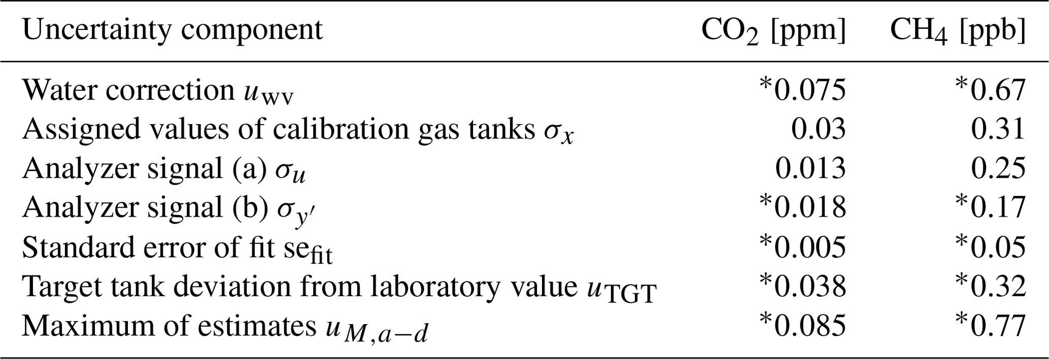

Figure E1Estimates of CO2 and CH4 measurement uncertainty as defined in Eqs. (E3)–(E6). The dashed lines are the WMO interlaboratory compatibility goals.
E3 Random and systematic uncertainty components
The uncertainty components described in Sects. E1 and E2 are mostly independent of the averaging period for which atmospheric data are reported (1 h). Rather, they describe systematic uncertainties inherent to the calibration procedure and long-term drift (σx, sefit, uTGT), and the water correction (uwv). Thus, these uncertainty estimates would not be smaller for atmospheric data averaged over longer periods. Exceptions are the analyzer signal precision estimates σu and , which contain random uncertainties: the precision model σu was estimated based on hourly averages and reflects both their uncertainty and drift on the timescale of 12 d. Thus, it might change for different averaging periods. The analyzer signal uncertainty estimate was sensitive to several timescales, i.e., 2 min (averaging period of calibration data), 22 min (time span of data of one calibration episode), 116 h (time between individual calibration episodes), and 120 d (averaging window for calibration coefficients). To investigate whether uncertainties at these timescales were similar to those of the hourly averages of atmospheric data, we computed the Allan deviations for CO2 and CH4. The uncertainties of averages over 2 min, 22 min, and 1 h were close (Fig. E2). In addition, the analyzer precision deteriorated beyond 1 h. These results are similar (qualitatively and quantitatively) to those documented by Yver Kwok et al. (2015) for several Picarro GHG analyzers.
The analyzer signal precision estimates only accounted for a small fraction of the total uncertainty (Table E1). Thus, the random uncertainty components play a minor role in the calibration of Ambarchik data, and averaging atmospheric data over different periods would not change the total estimated uncertainty considerably.
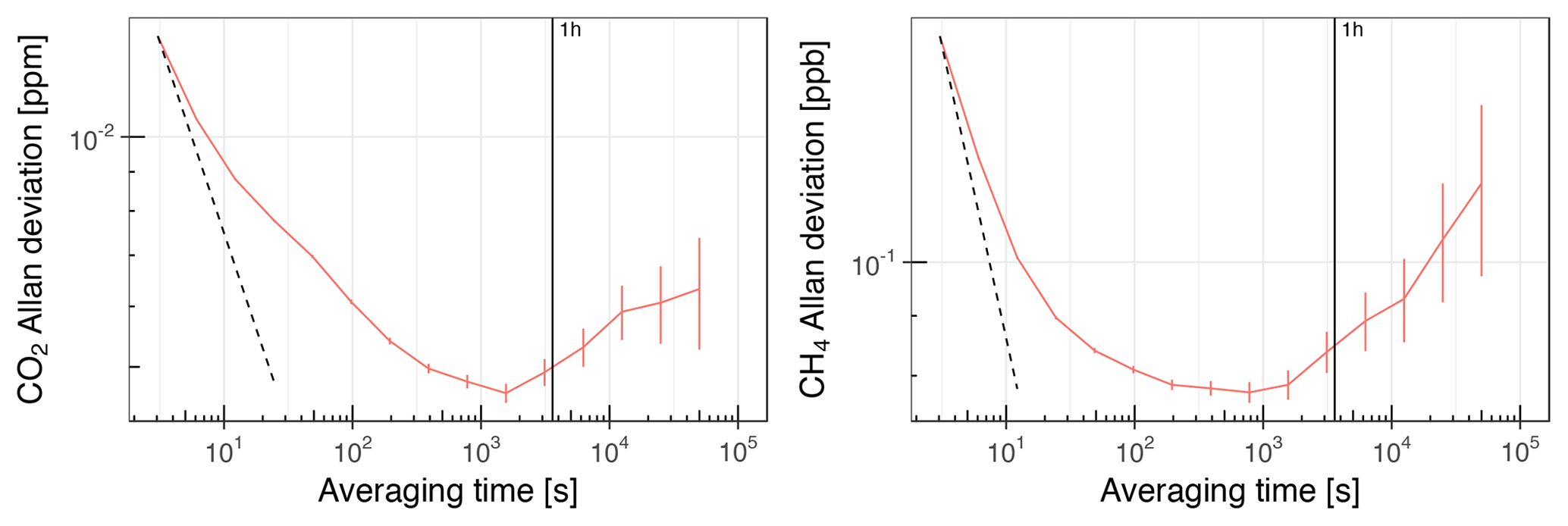
Figure E2Allan deviation of the CO2 and CH4 readings of the CRDS analyzer in Ambarchik. Values are based on one 12 d measurement of dry air from a gas tank in the lab prior to field deployment. The averaging time is cut off where the error becomes too large for a meaningful interpretation of the result. The vertical line denotes an averaging time of 1 h. The dashed line corresponds to white noise (slope −0.5), scaled to coincide with the first data point of the Allan deviation.
E4 Potential improvements of the calibration accuracy
Several aspects to the accuracy of the calibration using regular gas tank measurements are subject to future research. Here, we outline potential calibration errors that could not be conclusively quantified, and how we plan to address them in the future.
To investigate whether the regular probing time of the gas tanks was sufficient for equilibration (e.g., due to flushing of the tubing), we fitted exponential functions to the medians of the regular tank measurements. Deviations between modeled equilibrium mole fractions and the averages used for calibration were negligible ( < 0.008 ppm; < 0.09 ppb) and thus ignored. Furthermore, in two experiments, we investigated equilibration error and other drifts (e.g., diffusion in the pressure reducers) by measuring the calibration tanks in reversed order, and in original order for up to 2 h. However, the experiments were inconclusive. Based on the available data, we estimated the largest conceivable biases for the ranges 350–450 ppm CO2 and 1800–2400 ppb CH4. They were up to 0.06 ppm CO2 and 0.5 ppb CH4 at the edges of these ranges and vanished around their centers. An additional source of bias might be inlet pressure sensitivity of the Picarro analyzer as documented by Gomez-Pelaez et al. (2019). Using the sensitivities reported therein, some of the gas tank measurements in Ambarchik could have a bias of up to 0.03 ppm CO2 and 0.2 ppb CH4. More experiments are necessary to rule out or confirm and assess these possible biases; hence, no bias correction was implemented.
The CO2 bias of the water-corrected target tank mole fractions varied from −0.06 to −0.01 ppm (Fig. 5, top panel). These variations correlated with residual water vapor (which was much smaller than 0.01 %) and temperature in the laboratory during the target tank measurements, as well as with ambient CO2 mole fractions sampled before. This suggests that the variations may be due to insufficient flushing during calibration. However, the correlations varied over time without changes to the hardware or probing strategy. Therefore, further investigation of this observation is required, and no correction was implemented.
So far, possible drifts of the gas tanks could not be assessed and have therefore not been included in our uncertainty assessment. This will be assessed only when the gas tanks are almost empty, and shipped back to the MPI-BGC for recalibration.
MH, SZ and MG conceptualized the study. JVL, MH, OK, NZ, FR, and MG designed and set up the Ambarchik station. NZ and SZ coordinated setup and maintenance of the Ambarchik station. FR and MP performed calibration experiments. FR curated and analyzed the data. FR prepared the paper with contributions from all authors. MG supervised the project, and reviewed and edited the paper.
The authors declare that they have no conflict of interest.
This article is part of the special issue “The 10th International Carbon Dioxide Conference (ICDC10) and the 19th WMO/IAEA Meeting on Carbon Dioxide, other Greenhouse Gases and Related Measurement Techniques (GGMT-2017) (AMT/ACP/BG/CP/ESD inter-journal SI)”. It is a result of the 10th International Carbon Dioxide Conference, Interlaken, Switzerland, 21–25 August 2017.
The authors would like to thank Armin Jordan (MPI-BGC) for preparing the gas cylinders. We would also like to thank Christian Rödenbeck (MPI-BGC) for access to the Jena Inversion code for producing global CO2 mole fraction fields, Tonatiuh Guillermo Nuñez Ramirez (MPI-BGC) for providing global CH4 mole fraction fields, and John Henderson (AER) for providing footprints for Ambarchik. Lastly, the authors wish to thank NOAA GMD for making the CO2 and CH4 data from Barrow available.
This work was supported by the Max Planck Society, the European Commission
(PAGE21 project, FP7-ENV-2011, grant agreement no. 282700; PerCCOM project,
FP7-PEOPLE-2012-CIG, grant agreement no. PCIG12-GA-201-333796; INTAROS
project, H2020-BG-2016-2017, grant agreement no. 727890), the German
Ministry of Education and Research (CarboPerm Project, BMBF grant no.
03G0836G), the AXA Research Fund (PDOC_2012_W2
campaign, ARF fellowship Mathias Göckede), and the European Science
Foundation (TTorch Research Networking Programme, Short Visit Grant Friedemann
Reum).
The article processing charges for this open-access
publication were covered by the Max Planck Society.
This paper was edited by Christoph Zellweger and reviewed by two anonymous referees.
Andrews, A. E., Kofler, J. D., Trudeau, M. E., Williams, J. C., Neff, D. H., Masarie, K. A., Chao, D. Y., Kitzis, D. R., Novelli, P. C., Zhao, C. L., Dlugokencky, E. J., Lang, P. M., Crotwell, M. J., Fischer, M. L., Parker, M. J., Lee, J. T., Baumann, D. D., Desai, A. R., Stanier, C. O., De Wekker, S. F. J., Wolfe, D. E., Munger, J. W., and Tans, P. P.: CO2, CO, and CH4 measurements from tall towers in the NOAA Earth System Research Laboratory's Global Greenhouse Gas Reference Network: instrumentation, uncertainty analysis, and recommendations for future high-accuracy greenhouse gas monitoring efforts, Atmos. Meas. Tech., 7, 647–687, https://doi.org/10.5194/amt-7-647-2014, 2014.
Belshe, E. F., Schuur, E. A. G., and Bolker, B. M.: Tundra ecosystems observed to be CO2 sources due to differential amplification of the carbon cycle., Ecol. Lett., 16, 1307–1315, https://doi.org/10.1111/ele.12164, 2013.
Berchet, A., Bousquet, P., Pison, I., Locatelli, R., Chevallier, F., Paris, J.-D., Dlugokencky, E. J., Laurila, T., Hatakka, J., Viisanen, Y., Worthy, D. E. J., Nisbet, E., Fisher, R., France, J., Lowry, D., Ivakhov, V., and Hermansen, O.: Atmospheric constraints on the methane emissions from the East Siberian Shelf, Atmos. Chem. Phys., 16, 4147–4157, https://doi.org/10.5194/acp-16-4147-2016, 2016.
Chen, H., Winderlich, J., Gerbig, C., Hoefer, A., Rella, C. W., Crosson, E. R., Van Pelt, A. D., Steinbach, J., Kolle, O., Beck, V., Daube, B. C., Gottlieb, E. W., Chow, V. Y., Santoni, G. W., and Wofsy, S. C.: High-accuracy continuous airborne measurements of greenhouse gases (CO2 and CH4) using the cavity ring-down spectroscopy (CRDS) technique, Atmos. Meas. Tech., 3, 375–386, https://doi.org/10.5194/amt-3-375-2010, 2010.
Danielson, J. J. and Gesch, D. B.: Global Multi-resolution Terrain Elevation Data 2010 (GMTED2010), U.S. Geol. Surv. Open-File Rep. 2011–1073, 2010, 26, 2011.
Dlugokencky, E. J., Crotwell, A. M., Lang, P. M., and Mund, J. W.: Atmospheric Methane Dry Air Mole Fractions from quasi-continuous measurements at Barrow, Alaska and Mauna Loa, Hawaii, 1986–2016, Version: 2017-01-20, available at: ftp://aftp.cmdl.noaa.gov/data/trace_gases/ch4/in-situ/surface (last access: 26 June 2017), 2017.
El Yazidi, A., Ramonet, M., Ciais, P., Broquet, G., Pison, I., Abbaris, A., Brunner, D., Conil, S., Delmotte, M., Gheusi, F., Guerin, F., Hazan, L., Kachroudi, N., Kouvarakis, G., Mihalopoulos, N., Rivier, L., and Serça, D.: Identification of spikes associated with local sources in continuous time series of atmospheric CO, CO2 and CH4, Atmos. Meas. Tech., 11, 1599–1614, https://doi.org/10.5194/amt-11-1599-2018, 2018.
Euskirchen, E. S., Bret-Harte, M. S., Scott, G. J., Edgar, C., and Shaver, G. R.: Seasonal patterns of carbon dioxide and water fluxes in three representative tundra ecosystems in northern Alaska, Ecosphere, 3, 1–19, https://doi.org/10.1890/ES11-00202.1, 2012.
Gomez-Pelaez, A. J., Ramos, R., Cuevas, E., Gomez-Trueba, V., and Reyes, E.: Atmospheric CO2, CH4, and CO with the CRDS technique at the Izaña Global GAW station: instrumental tests, developments, and first measurement results, Atmos. Meas. Tech., 12, 2043–2066, https://doi.org/10.5194/amt-12-2043-2019, 2019.
Goodrich, J. P., Oechel, W. C., Gioli, B., Moreaux, V., Murphy, P. C., Burba, G., and Zona, D.: Impact of different eddy covariance sensors, site set-up, and maintenance on the annual balance of CO2 and CH4 in the harsh Arctic environment, Agric. For. Meteorol., 228–229, 239–251, https://doi.org/10.1016/j.agrformet.2016.07.008, 2016.
Henderson, J. M., Eluszkiewicz, J., Mountain, M. E., Nehrkorn, T., Chang, R. Y.-W., Karion, A., Miller, J. B., Sweeney, C., Steiner, N., Wofsy, S. C., and Miller, C. E.: Atmospheric transport simulations in support of the Carbon in Arctic Reservoirs Vulnerability Experiment (CARVE), Atmos. Chem. Phys., 15, 4093–4116, https://doi.org/10.5194/acp-15-4093-2015, 2015.
Hugelius, G., Strauss, J., Zubrzycki, S., Harden, J. W., Schuur, E. A. G., Ping, C.-L., Schirrmeister, L., Grosse, G., Michaelson, G. J., Koven, C. D., O'Donnell, J. A., Elberling, B., Mishra, U., Camill, P., Yu, Z., Palmtag, J., and Kuhry, P.: Estimated stocks of circumpolar permafrost carbon with quantified uncertainty ranges and identified data gaps, Biogeosciences, 11, 6573–6593, https://doi.org/10.5194/bg-11-6573-2014, 2014.
IPCC: Climate Change 2013, The Physical Science Basis, Working Group 1 Contribution to the Fifth Assessment Report of the Intergovernmental Panel on Climate Change, 2013.
James, R. H., Bousquet, P., Bussmann, I., Haeckel, M., Kipfer, R., Leifer, I., Niemann, H., Ostrovsky, I., Piskozub, J., Rehder, G., Treude, T., Vielstädte, L., and Greinert, J.: Effects of climate change on methane emissions from seafloor sediments in the Arctic Ocean: A review, Limnol. Oceanogr., 61, 283–299, https://doi.org/10.1002/lno.10307, 2016.
Jeong, S.-J., Bloom, A. A., Schimel, D., Sweeney, C., Parazoo, N. C., Medvigy, D., Schaepman-Strub, G., Zheng, C., Schwalm, C. R., Huntzinger, D. N., Michalak, A. M., and Miller, C. E.: Accelerating rates of Arctic carbon cycling revealed by long-term atmospheric CO2 measurements, Sci. Adv., 4, eaao1167, https://doi.org/10.1126/sciadv.aao1167, 2018.
Kittler, F., Burjack, I., Corradi, C. A. R., Heimann, M., Kolle, O., Merbold, L., Zimov, N., Zimov, S., and Göckede, M.: Impacts of a decadal drainage disturbance on surface–atmosphere fluxes of carbon dioxide in a permafrost ecosystem, Biogeosciences, 13, 5315–5332, https://doi.org/10.5194/bg-13-5315-2016, 2016.
Kittler, F., Eugster, W., Foken, T., Heimann, M., Kolle, O., and Göckede, M.: High-quality eddy-covariance CO2 budgets under cold climate conditions, J. Geophys. Res.-Biogeo., 122, 2064–2084, https://doi.org/10.1002/2017JG003830, 2017a.
Kittler, F., Heimann, M., Kolle, O., Zimov, N., Zimov, S. A., and Göckede, M.: Long-Term Drainage Reduces CO2 Uptake and CH4 Emissions in a Siberian Permafrost Ecosystem, Global Biogeochem. Cy., 31, 1704–1717, https://doi.org/10.1002/2017GB005774, 2017b.
Kwon, M. J., Beulig, F., Ilie, I., Wildner, M., Küsel, K., Merbold, L., Mahecha, M. D., Zimov, N., Zimov, S. A., Heimann, M., Schuur, E. A. G., Kostka, J. E., Kolle, O., Hilke, I., and Göckede, M.: Plants, microorganisms, and soil temperatures contribute to a decrease in methane fluxes on a drained Arctic floodplain, Glob. Change Biol., 23, 2396–2412, https://doi.org/10.1111/gcb.13558, 2017.
Lin, J. C., Gerbig, C., Wofsy, S. C., Andrews, A. E., Daube, B. C., Davis, K. J., and Grainger, C. A.: A near-field tool for simulating the upstream influence of atmospheric observations: The Stochastic Time-Inverted Lagrangian Transport (STILT) model, J. Geophys. Res., 108, 4493, https://doi.org/10.1029/2002JD003161, 2003.
Masarie, K. A., Pétron, G., Andrews, A. E., Bruhwiler, L., Conway, T. J., Jacobson, A. R., Miller, J. B., Tans, P. P., Worthy, D. E. J., and Peters, W.: Impact of CO2 measurement bias on CarbonTracker surface flux estimates, J. Geophys. Res.-Atmos., 116, 1–13, https://doi.org/10.1029/2011JD016270, 2011.
Mastepanov, M., Sigsgaard, C., Dlugokencky, E. J., Houweling, S., Ström, L., Tamstorf, M. P., and Christensen, T. R.: Large tundra methane burst during onset of freezing, Nature, 456, 628–630, https://doi.org/10.1038/nature07464, 2008.
Mastepanov, M., Sigsgaard, C., Tagesson, T., Ström, L., Tamstorf, M. P., Lund, M., and Christensen, T. R.: Revisiting factors controlling methane emissions from high-Arctic tundra, Biogeosciences, 10, 5139–5158, https://doi.org/10.5194/bg-10-5139-2013, 2013.
McGuire, A. D., Christensen, T. R., Hayes, D., Heroult, A., Euskirchen, E., Kimball, J. S., Koven, C., Lafleur, P., Miller, P. A., Oechel, W., Peylin, P., Williams, M., and Yi, Y.: An assessment of the carbon balance of Arctic tundra: comparisons among observations, process models, and atmospheric inversions, Biogeosciences, 9, 3185–3204, https://doi.org/10.5194/bg-9-3185-2012, 2012.
Miller, S. M., Worthy, D. E. J., Michalak, A. M., Wofsy, S. C., Kort, E. A., Havice, T. C., Andrews, A. E., Dlugokencky, E. J., Kaplan, J. O., Levi, P. J., Tian, H., and Zhang, B.: Observational constraints on the distribution, seasonality, and environmental predictors of North American boreal methane emissions, Global Biogeochem. Cy., 28, 146–160, https://doi.org/10.1002/2013GB004580, 2014.
NOAA: Atmospheric Carbon Dioxide Dry Air Mole Fractions from quasi-continuous measurements at Barrow, Alaska, Compiled by Thoning, K. W., Kitzis, D. R., and Crotwell, A., National Oceanic and Atmospheric Administration (NOAA), Earth System Research Laboratory (ESRL), Global Monitoring Division (GMD): Boulder, Colorado, USA, Version 2015-12 at https://doi.org/10.7289/V5RR1W6B, 2015.
Oechel, W. C., Laskowski, C. A., Burba, G., Gioli, B., and Kalhori, A. A. M.: Annual patterns and budget of CO2 flux in an Arctic tussock tundra ecosystem, J. Geophys. Res.-Biogeo., 119, 323–339, https://doi.org/10.1002/2013JG002431, 2014.
Olson, D. M., Dinerstein, E., Wikramanayake, E. D., Burgess, N. D., Powell, G. V. N., Underwood, E. C., D'amico, J. A., Itoua, I., Strand, H. E., Morrison, J. C., Loucks, C. J., Allnutt, T. F., Ricketts, T. H., Kura, Y., Lamoreux, J. F., Wettengel, W. W., Hedao, P., and Kassem, K. R.: Terrestrial Ecoregions of the World: A New Map of Life on Earth, Bioscience, 51, 933, https://doi.org/10.1641/0006-3568(2001)051[0933:TEOTWA]2.0.CO;2, 2001.
Park, T., Ganguly, S., Tømmervik, H., Euskirchen, E. S., Høgda, K.-A., Karlsen, S. R., Brovkin, V., Nemani, R. R., and Myneni, R. B.: Changes in growing season duration and productivity of northern vegetation inferred from long-term remote sensing data, Environ. Res. Lett., 11, 84001, https://doi.org/10.1088/1748-9326/11/8/084001, 2016.
Peters, W., Krol, M. C., van der Werf, G. R., Houweling, S., Jones, C. D., Hughes, J., Schaefer, K., Masarie, K. A., Jacobson, A. R., Miller, J. B., Cho, C. H., Ramonet, M., Schmidt, M., Ciattaglia, L., Apadula, F., Heltai, D., Meinhardt, F., di Sarra, A. G., Piacentino, S., Sferlazzo, D., Aalto, T., Hatakka, J., Ström, J., Haszpra, L., Meijer, H. A. J., van Der Laan, S., Neubert, R. E. M., Jordan, A., Rodó, X., Morguí, J. A., Vermeulen, A. T., Popa, E., Rozanski, K., Zimnoch, M., Manning, A. C., Leuenberger, M., Uglietti, C., Dolman, A. J., Ciais, P., Heimann, M., and Tans, P. P.: Seven years of recent European net terrestrial carbon dioxide exchange constrained by atmospheric observations, Glob. Change Biol., 16, 1317–1337, https://doi.org/10.1111/j.1365-2486.2009.02078.x, 2010.
Rella, C. W., Chen, H., Andrews, A. E., Filges, A., Gerbig, C., Hatakka, J., Karion, A., Miles, N. L., Richardson, S. J., Steinbacher, M., Sweeney, C., Wastine, B., and Zellweger, C.: High accuracy measurements of dry mole fractions of carbon dioxide and methane in humid air, Atmos. Meas. Tech., 6, 837–860, https://doi.org/10.5194/amt-6-837-2013, 2013.
Reum, F., Gerbig, C., Lavric, J. V., Rella, C. W., and Göckede, M.: Correcting atmospheric CO2 and CH4 mole fractions obtained with Picarro analyzers for sensitivity of cavity pressure to water vapor, Atmos. Meas. Tech., 12, 1013–1027, https://doi.org/10.5194/amt-12-1013-2019, 2019.
Rienecker, M. M., Suarez, M. J., Gelaro, R., Todling, R., Bacmeister, J., Liu, E., Bosilovich, M. G., Schubert, S. D., Takacs, L., Kim, G. K., Bloom, S., Chen, J., Collins, D., Conaty, A., Da Silva, A., Gu, W., Joiner, J., Koster, R. D., Lucchesi, R., Molod, A., Owens, T., Pawson, S., Pegion, P., Redder, C. R., Reichle, R., Robertson, F. R., Ruddick, A. G., Sienkiewicz, M., and Woollen, J.: MERRA: NASA's modern-era retrospective analysis for research and applications, J. Climate, 24, 3624–3648, https://doi.org/10.1175/JCLI-D-11-00015.1, 2011.
Rödenbeck, C.: Estimating CO2 sources and sinks from atmospheric mixing ratio measurements using a global inversion of atmospheric transport, Technical report, Max-Planck-Institute for Biogeochemistry, Jena, 2005.
Rödenbeck, C., Houweling, S., Gloor, M., and Heimann, M.: CO2 flux history 1982–2001 inferred from atmospheric data using a global inversion of atmospheric transport, Atmos. Chem. Phys., 3, 1919–1964, https://doi.org/10.5194/acp-3-1919-2003, 2003.
Rödenbeck, C., Conway, T. J., and Langenfelds, R. L.: The effect of systematic measurement errors on atmospheric CO2 inversions: a quantitative assessment, Atmos. Chem. Phys., 6, 149–161, https://doi.org/10.5194/acp-6-149-2006, 2006.
Schuur, E. A. G., Abbott, B. W., Bowden, W. B., Brovkin, V., Camill, P., Canadell, J. G., Chanton, J. P., Chapin, F. S., Christensen, T. R., Ciais, P., Crosby, B. T., Czimczik, C. I., Grosse, G., Harden, J., Hayes, D. J., Hugelius, G., Jastrow, J. D., Jones, J. B., Kleinen, T., Koven, C. D., Krinner, G., Kuhry, P., Lawrence, D. M., McGuire, A. D., Natali, S. M., O'Donnell, J. A., Ping, C. L., Riley, W. J., Rinke, A., Romanovsky, V. E., Sannel, A. B. K., Schädel, C., Schaefer, K., Sky, J., Subin, Z. M., Tarnocai, C., Turetsky, M. R., Waldrop, M. P., Walter Anthony, K. M., Wickland, K. P., Wilson, C. J., and Zimov, S. A.: Expert assessment of vulnerability of permafrost carbon to climate change, Clim. Change, 119, 359–374, https://doi.org/10.1007/s10584-013-0730-7, 2013.
Schuur, E. A. G., McGuire, A. D., Schädel, C., Grosse, G., Harden, J. W., Hayes, D. J., Hugelius, G., Koven, C. D., Kuhry, P., Lawrence, D. M., Natali, S. M., Olefeldt, D., Romanovsky, V. E., Schaefer, K., Turetsky, M. R., Treat, C. C., and Vonk, J. E.: Climate change and the permafrost carbon feedback, Nature, 520, 171–179, https://doi.org/10.1038/nature14338, 2015.
Shakhova, N. E., Semiletov, I. P., Leifer, I., Sergienko, V., Salyuk, A., Kosmach, D., Chernykh, D., Stubbs, C., Nicolsky, D., Tumskoy, V., and Gustafsson, Ö.: Ebullition and storm-induced methane release from the East Siberian Arctic Shelf, Nat. Geosci., 7, 64–70, https://doi.org/10.1038/ngeo2007, 2014.
Skamarock, W. C., Klemp, J. B., Dudhi, J., Gill, D. O., Barker, D. M., Duda, M. G., Huang, X.-Y., Wang, W., and Powers, J. G.: A Description of the Advanced Research WRF Version 3, NCAR Technical Note NCAR/TN-475+STR, 2008.
Stavert, A. R., O'Doherty, S., Stanley, K., Young, D., Manning, A. J., Lunt, M. F., Rennick, C., and Arnold, T.: UK greenhouse gas measurements at two new tall towers for aiding emissions verification, Atmos. Meas. Tech., 12, 4495–4518, https://doi.org/10.5194/amt-12-4495-2019, 2019.
Stull, R. B.: An Introduction to Boundary Layer Meteorology, Springer Netherlands, Dordrecht, 1988.
Sweeney, C., Dlugokencky, E., Miller, C. E., Wofsy, S., Karion, A., Dinardo, S., Chang, R. Y.-W., Miller, J. B., Bruhwiler, L., Crotwell, A. M., Newberger, T., McKain, K., Stone, R. S., Wolter, S. E., Lang, P. E., and Tans, P.: No significant increase in long-term CH4 emissions on North Slope of Alaska despite significant increase in air temperature, Geophys. Res. Lett., 43, 6604–6611, https://doi.org/10.1002/2016GL069292, 2016.
Taylor, J. R.: An Introduction to Error Analysis, 2nd edn., University Science Books, Sausalito, CA, 1997.
Thompson, R. L., Sasakawa, M., Machida, T., Aalto, T., Worthy, D., Lavric, J. V., Lund Myhre, C., and Stohl, A.: Methane fluxes in the high northern latitudes for 2005–2013 estimated using a Bayesian atmospheric inversion, Atmos. Chem. Phys., 17, 3553–3572, https://doi.org/10.5194/acp-17-3553-2017, 2017.
Thoning, K. W., Tans, P. P., and Komhyr, W. D.: Atmospheric carbon dioxide at Mauna Loa Observatory: 2. Analysis of the NOAA GMCC data, 1974–1985, J. Geophys. Res., 94, 8549, https://doi.org/10.1029/JD094iD06p08549, 1989.
Thornton, B. F., Geibel, M. C., Crill, P. M., Humborg, C., and Mörth, C. M.: Methane fluxes from the sea to the atmosphere across the Siberian shelf seas, Geophys. Res. Lett., 43, 5869–5877, https://doi.org/10.1002/2016GL068977, 2016.
Vickers, D. and Mahrt, L.: Quality Control and Flux Sampling Problems for Tower and Aircraft Data, J. Atmos. Ocean. Tech., 14, 512–526, https://doi.org/10.1175/1520-0426(1997)014<0512:QCAFSP>2.0.CO;2, 1997.
Weatherall, P., Marks, K. M., Jakobsson, M., Schmitt, T., Tani, S., Arndt, J. E., Rovere, M., Chayes, D., Ferrini, V., and Wigley, R.: A new digital bathymetric model of the world's oceans, Earth Sp. Sci., 2, 331–345, https://doi.org/10.1002/2015EA000107, 2015.
WMO: 18th WMO/IAEA Meeting on Carbon Dioxide, Other Greenhouse Gases and Related Tracers Measurement Techniques (GGMT-2015), available at: https://library.wmo.int/opac/doc_num.php?explnum_id=3074 (last access: 30 May 2017), 2016.
Yver Kwok, C., Laurent, O., Guemri, A., Philippon, C., Wastine, B., Rella, C. W., Vuillemin, C., Truong, F., Delmotte, M., Kazan, V., Darding, M., Lebègue, B., Kaiser, C., Xueref-Rémy, I., and Ramonet, M.: Comprehensive laboratory and field testing of cavity ring-down spectroscopy analyzers measuring H2O, CO2, CH4 and CO, Atmos. Meas. Tech., 8, 3867–3892, https://doi.org/10.5194/amt-8-3867-2015, 2015.
Zona, D., Gioli, B., Commane, R., Lindaas, J., Wofsy, S. C., Miller, C. E., Dinardo, S. J., Dengel, S., Sweeney, C., Karion, A., Chang, R. Y.-W., Henderson, J. M., Murphy, P. C., Goodrich, J. P., Moreaux, V., Liljedahl, A., Watts, J. D., Kimball, J. S., Lipson, D. A., and Oechel, W. C.: Cold season emissions dominate the Arctic tundra methane budget, P. Natl. Acad. Sci. USA, 113, 40–45, https://doi.org/10.1073/pnas.1516017113, 2016.
- Abstract
- Introduction
- Station description
- Quality control
- Atmospheric tracer transport to Ambarchik
- Greenhouse gas signals at Ambarchik
- Discussion and conclusions
- Data availability
- Appendix A: Hardware manufacturers and models
- Appendix B: Derivation of water correction coefficients
- Appendix C: Calibration scale and coefficients
- Appendix D: Spike detection algorithm for CO2
- Appendix E: Measurement uncertainties
- Author contributions
- Competing interests
- Special issue statement
- Acknowledgements
- Financial support
- Review statement
- References