the Creative Commons Attribution 4.0 License.
the Creative Commons Attribution 4.0 License.
 | 05 Dec 2019
Estimation of turbulence dissipation rate from Doppler wind lidars and in situ instrumentation for the Perdigão 2017 campaign
Nicola Bodini
Julie K. Lundquist
Ludovic Bariteau
Johannes Wagner
The understanding of the sources, spatial distribution and temporal variability of turbulence in the atmospheric boundary layer, and improved simulation of its forcing processes require observations in a broad range of terrain types and atmospheric conditions. In this study, we estimate turbulence kinetic energy dissipation rate ε using multiple techniques, including in situ measurements of sonic anemometers on meteorological towers, a hot-wire anemometer on a tethered lifting system and remote-sensing retrievals from a vertically staring lidar and two lidars performing range–height indicator (RHI) scans. For the retrieval of ε from the lidar RHI scans, we introduce a modification of the Doppler spectral width method. This method uses spatiotemporal averages of the variance in the line-of-sight velocity and the turbulent broadening of the Doppler backscatter spectrum. We validate this method against the observations from the other instruments, also including uncertainty estimations for each method. The synthesis of the results from all instruments enables a detailed analysis of the spatial and temporal variability in ε across a valley between two parallel ridges at the Perdigão 2017 campaign. We analyze in detail how ε varies in the night from 13 to 14 June 2017. We find that the shear zones above and below a nighttime low-level jet experience turbulence enhancements. We also show that turbulence in the valley, approximately 11 rotor diameters downstream of an operating wind turbine, is still significantly enhanced by the wind turbine wake.
- Article
(5611 KB) - Full-text XML
-
Supplement
(2757 KB) - BibTeX
- EndNote


The copyright of the authors Norman Wildmann and Johannes Wagner for this publication is transferred to Deutsches Zentrum für Luft- und Raumfahrt e.V., the German Aerospace Center. Alliance for Sustainable Energy, LLC (Alliance) is the manager and operator of the National Renewable Energy Laboratory (NREL). Employees of Alliance for Sustainable Energy, LLC, under Contract No. DE-AC36-08GO28308 with the U.S. Dept. of Energy, have authored this work in part. The United States Government retains and the publisher, by accepting the article for publication, acknowledges that the United States Government retains a nonexclusive, paid-up, irrevocable, worldwide license to publish or reproduce the published form of this work, for United States Government purposes.
Turbulence is the major driving force for mixing in the atmospheric boundary layer (ABL) and an essential flow property. Parameterizations of turbulence underpin all weather forecasting models (e.g. see Nakanishi and Niino, 2006), yet these parameterizations have shown to be a source of large uncertainties in flow modeling. Goger et al. (2018) found that in the COSMO model, turbulence kinetic energy (TKE) is systematically underestimated with a one-dimensional turbulence parameterization. Recent sensitivity studies by Yang et al. (2017) showed that the parameters associated with turbulent mixing in an ABL parametrization have a large impact on 80 m wind speeds in the Weather Research and Forecasting model (WRF). They find that parameters associated with turbulence dissipation rate are responsible for approximately 50 % of the variance in 80 m wind speeds. Muñoz-Esparza et al. (2018) used turbulence measurements from sonic anemometers at the XPIA campaign (Lundquist et al., 2017) to motivate improvements in WRF boundary-layer parameterizations.
Part of the challenge for both observational capabilities and for subgrid-scale turbulence modeling is the wide range of mechanisms that can generate turbulence: in stable atmospheric conditions, wavelike motions cause intermittent turbulence which is only poorly understood (Sun et al., 2015). Convection and thermally driven flows are equally challenging with turbulence occurring on different scales (Adler and Kalthoff, 2014). In heterogeneous, complex terrains, very specific phenomena occur such as recirculation or detachment caused by mountains (Stull, 1988; Menke et al., 2019) or blockage at the edges of forests or other obstacles (Irvine et al., 1997; Dupont and Brunet, 2009; Mann and Dellwik, 2014). In highly complex terrain sites, forests or patches of trees with varying canopy densities and heights induce variable mixing processes (Belcher et al., 2012). In contrast to these natural sources of turbulence, wind turbines generate vortices at the rotor blades which propagate downstream and disperse in a wake, a region of high turbulence which interacts with the surrounding atmosphere (Lundquist and Bariteau, 2015).
While observations are essential to improve our understanding and simulation of turbulent processes, the retrieval of turbulence parameters from measurements is not trivial, especially for complex sites. Sonic anemometers are a reliable tool to resolve the small scales of turbulence, allowing the calculation of turbulence parameters at fixed points in space (Champagne, 1978; Oncley et al., 1996; Beyrich et al., 2006). However, point measurements are not necessarily representative of turbulent mixing in a larger area, which is especially critical above the surface layer in the presence of convective rolls (Maurer et al., 2016). Recent developments in commercial scanning lidars can provide an assessment of turbulent mixing over a broader region (Smalikho et al., 2013), and many different methods have been introduced to retrieve vertical profiles of turbulence from either vertical stare measurements (O’Connor et al., 2010; Bodini et al., 2018, 2019; Wilczak et al., 2019), six-beam scanning scenarios (Sathe et al., 2015; Bonin et al., 2017), or velocity–azimuth display scans (VAD; Eberhard et al., 1989; Smalikho and Banakh, 2017). Krishnamurthy et al. (2011) derived vertical profiles of TKE from horizontal plan-position indicator (PPI) scans (see also Wilczak et al., 2019). Various methods also exist to retrieve vertical profiles of turbulence from range–height indicator (RHI) scans in homogeneous, flat terrains (Smalikho et al., 2005; Bonin et al., 2017). Using more than one lidar, multi-Doppler retrievals of the three-dimensional wind vector are possible and the obtained wind data can be analyzed for turbulence parameters (Newsom et al., 2008; Röhner and Träumner, 2013; Iungo and Porté-Agel, 2014; Pauscher et al., 2016; Wildmann et al., 2018b).
Here we demonstrate a new approach for assessing the variability of turbulence parameters in a complex terrain by employing multiple instruments to provide a comprehensive view of turbulence structures and variability at the Perdigão 2017 field campaign (details in Sect. 2). A new method is introduced to retrieve TKE dissipation rate ε from lidar range–height indicator (RHI) scans, which allow for a two-dimensional perspective of the turbulence in the valley between two ridges. These retrievals are calibrated with data from sonic anemometers on meteorological towers and validated with more established measurements of ε from lidar vertical stare measurements and high-resolution hot-wire anemometer measurements on a tethered lifting system (TLS). The goal of this study is to demonstrate the opportunities that spatially distributed measurements of turbulence provide at a complex site as it is found in Perdigão while at the same time giving an elaborate estimation of uncertainties and limitations with the specific methods and experimental setup.
The different approaches to retrieve TKE dissipation rates are explained in Sect. 3 and results of the validation are given in Sect. 4. In Sect. 5, a case study is presented of a nighttime ABL featuring a low-level jet (LLJ) and a wind turbine wake. Both phenomena are sources of increased turbulence in the observed valley flow. An assessment of the data quality and results is given in Sect. 6. Prospects for future research and development are highlighted in the Conclusions section.
2.1 The site
Perdigão is a village in central Portugal, approximately 25 km west of Castelo Branco and eponymous for an international field campaign with the goal of studying the microscale flow over two nearly parallel mountain ridges. The two mountain ridges at Perdigão are oriented approximately 35∘ from north in the counterclockwise direction, running from northwest to southeast for an approximate distance of 1400 m. Figure 1 shows a map of the experimental site, rotated by 35∘ and focusing on the Vale do Cobrão in between the two mountain ridges. According to long-term measurements before the field campaign, the primary wind direction at the site is southwesterly, perpendicular to the ridge orientation (Fernando et al., 2019). A secondary wind pattern, that mainly occurs during nighttime, is the northeasterly flow, also perpendicular to the ridges. Wagner et al. (2019a) provide a detailed analysis of the meteorological situation during the period of intensive operation (IOP) of the campaign from 1 May to 15 June 2017. To visualize the complexity of the site not only in terms of the topography but also in terms of land use, roughness elements derived from a high-resolution aerial laser scan have been added to the map and show the patchwork of small areas of trees and forest. The vegetation data were collected in March 2016, approximately 1 year before the campaign, so because of rapid vegetation growth these data do not exactly represent vegetation heights during the IOP. A picture showing an aerial view of the site during the campaign can be seen in Fig. 2.
After initial pre-studies at the site (see Vasiljević et al., 2017), the 2017 campaign brought together a number of researchers interested in the microscale of complex terrain flows. A comprehensive description of the scientific goals of all contributing partners, as well as an overview of the instrumentation installed in the campaign, can be found in Fernando et al. (2019). The 195 sonic anemometers on 49 meteorological masts and 26 lidar systems of different kinds were installed to sample the complex three-dimensional flows in the valley between the mountain ridges as well as in the inflow and outflow regions.

Figure 1Map of the Vale do Cobrão. The gray structures are surface elements (mostly forest) obtained from a high-resolution lidar elevation scan 1 year before the campaign. The small map in the top-left corner gives a wider overview of the surrounding area. The dashed lines show the cross sections for measurements with the lidar instruments used in this study.
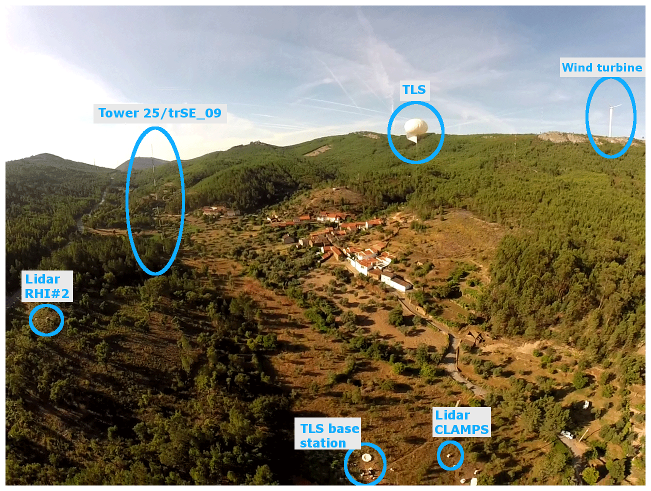
Figure 2Aerial view over the measurement site from the north.
2.2 Instrumentation
2.2.1 Sonic anemometers on meteorological masts
Out of the 195 sonic anemometers, this study relies on the instruments on towers 20/trSE_04 and 25/trSE_09. Both of these towers were 100 m high with sonic anemometers at 10, 20, 30, 40, 60, 80, and 100 m levels on booms pointing to ∼135∘ () for tower 20/trSE_04 (25/trSE_09). All sonic anemometers on these two masts were Gill WM Pro sonic anemometers, sampling the three-dimensional wind vector at a rate of 20 Hz. The two sonic anemometers at 80 and 100 m at the 100 m meteorological mast 25/trSE_09 were within the height limits of the lidar scans and are therefore used for intercomparison of turbulence measurements. The ground levels of towers 20/trSE_04 and 25/trSE_09 with respect to ridge height (i.e. wind turbine base height) are −10 and −178 m, respectively.
2.2.2 Tethered lifting system
The University of Colorado Boulder’s tethered lifting system (TLS), a specially designed tethersonde system, enables unique in situ high-rate measurements of wind speed, wind direction, and temperature. From these high-rate measurements, the TKE dissipation rate can be estimated (Frehlich et al., 2003, 2008). TLS capabilities for observing detailed wind speed, temperature, and dissipation rate profiles have been demonstrated in several field campaigns (Balsley et al., 2003; Frehlich et al., 2008), including measurements of dissipation rate in wind turbine wakes (Lundquist and Bariteau, 2015). Muschinski et al. (2004) used data from the TLS to assess small-scale and large-scale turbulence intermittency in flat terrain, while Sorbjan and Balsley (2008) used the system to explore microscale turbulence in the stable boundary layer.
The Perdigão TLS instrument packages were similar to those of Frehlich et al. (2008). Fast wind speed measurements at 1 kHz were from 1.25 mm length, 5 µm diameter, tungsten wires. Other measurements included 1 kHz cold-wire anemometer temperature measurements (Auspex Scientific, custom-made device), 100 Hz thermistors (Honeywell 111-103EAJ-H01), solid-state measurements for temperature (Analog Devices Inc TMP36) and relative humidity (Honeywell HIH-4000), a 100 Hz Pitot tube (Dwyer Instruments, model 166-6), and a pressure sensor (Honeywell DC001NDC4) for velocity and pressure measurements, as well as GPS and compass measurements. GPS measurements of latitude, longitude, and altitude were sampled every 5 s. While the TLS can be deployed in either a profiling or a hovering mode, most Perdigão measurements consisted of profiles. The ascent and descent of the TLS was controlled by a custom-made winch system with an average ascent and descent rate of 0.3 m s−1. The payloads were lifted using a 16 m3 Helikite system (Allsopp) with a lightweight but strong tether (1120 kg Dyneema line, 2.5 mm diameter).
2.2.3 Scanning lidars
Here we focus on the flow in the center of the valley and in a cross section through the location of the wind turbine. For this purpose, three Leosphere Windcube 200S lidars of the German Aerospace Center (DLR) were deployed at the locations indicated in Fig. 1. All of the systems performed RHI scans as indicated by the dashed lines in Fig. 1. Lidar RHI#1 and RHI#2 were aligned with the wind turbine along the primary wind direction. RHI#2, in the valley, probed the flow with a high elevation angle so that the line-of-sight (LOS) measurements included a significant contribution from the vertical wind component. RHI#1, on the northeast ridge, probed the valley flow at a low elevation angle, thus measuring primarily contributions of the horizontal wind components. Synthesizing data from these two lidars allows for coplanar wind speed retrievals as described in Wildmann et al. (2018a). RHI#3 provided additional information about the out-of-plane flow and wind turbine (WT) wake position. A combination of the three lidars also allowed multi-Doppler measurements of the wind turbine wake for a range of wind directions far from the main wind direction (Wildmann et al., 2018b). The parameters of the RHI scans and lidar specifications are given in Table 1. The horizontal distance from the masts, and thus the sonic anemometers, to the RHI plane of lidars RHI#1 and RHI#2 is 150 m.
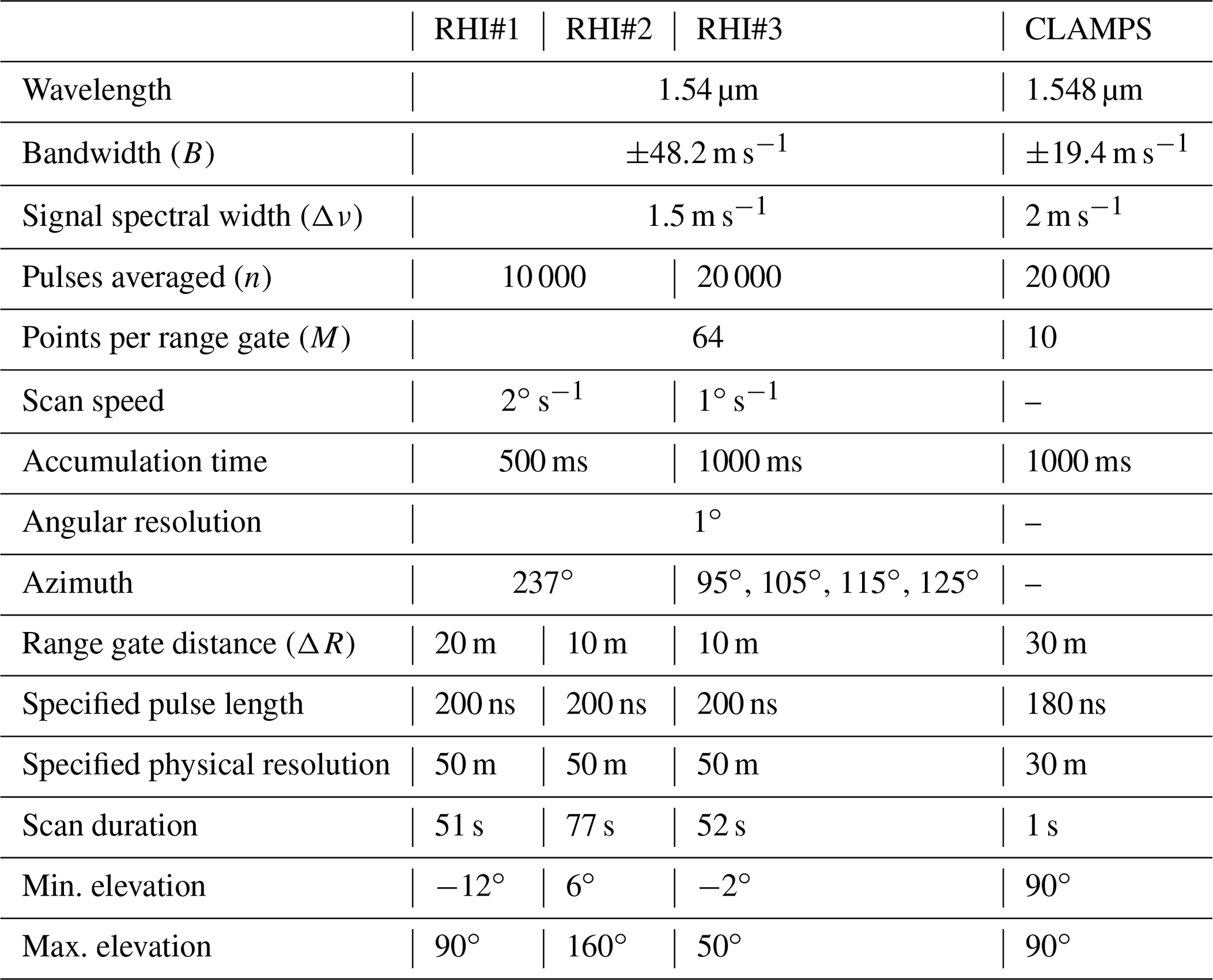
As part of the Collaborative Lower Atmospheric Mobile Profiling System (CLAMPS; Wagner et al., 2019b), the University of Oklahoma (OU) deployed a Halo Photonics Stream Line scanning lidar at the so-called Lower Orange site in the Vale do Cobrão, approximately 100 m from the cross section through the WT. The scanning scenarios for this lidar during the campaign comprised a regular sequence of velocity–azimuth display (VAD) scans (2 min), RHI along-valley (2 min) and cross-valley scans (2 min), and vertical stare measurements (9 min). In this study, the vertical stare measurements are used to derive turbulence dissipation rate and the results from the VAD scan is used for wind speed information. Table 1 gives an overview of the CLAMPS lidar parameters for the vertical stare measurements that are relevant for the turbulence retrieval (see Sect. 3). The horizontal distance of CLAMPS to the sonic anemometers on tower 25/trSE_09 is 250 m.
2.2.4 Radiosondes
From the valley, radiosondes were launched regularly every 6 h, aiming to reach 20 km at 00:00, 06:00, 12:00, and 18:00 UTC. The radiosondes provide vertical profiles of pressure, temperature, and humidity as well as wind speed and wind direction.
3.1 Basic equations and terminology
The quantification of turbulence from measured data in boundary-layer meteorology is often based on the assumption of homogeneity and local isotropy in the small scales of turbulence, which has been found to be valid in high Reynolds number flows (Kolmogorov, 1941). Under these assumptions, the energy cascade of eddies from larger to smaller scales in the inertial subrange of turbulence can be defined by a model for the energy spectral density S(κ):
where κ is the wave number, ε is the TKE dissipation rate, and α is a universal constant. Integration of the energy spectrum yields the variance σ2:
Turbulence of the velocity field can be described by the structure function D, which can be calculated from flow velocities v as the square of differences at spatially separated points:
where r is the separation distance and 〈 〉 is used to symbolize the ensemble average. By invoking Taylor's hypothesis of frozen turbulence, a separation distance can be converted to a separation time in a homogeneous flow with a mean flow velocity so that and
Kolmogorov (1941) formulated that the structure function scales with dissipation rate ε and the Kolmogorov constant Ck≈2 according to
Smalikho et al. (2005) derived the longitudinal spectrum of flow velocity from the Kolmogorov laws to yield
A characteristic length scale for turbulence is the integral length scale Lv. The integral length scale describes the scale over which turbulence remains correlated (Kaimal and Finnigan, 1994) and is defined as
where Bv(r) is the correlation function of flow velocity.
A model for atmospheric turbulence that extends to larger scales than the inertial subrange is the von Kármán model (von Kármán, 1948) which relates energy spectral density to the velocity variance and the integral length scale Lv:
3.2 Techniques to estimate turbulence dissipation rate
3.2.1 Sonic anemometers
TKE dissipation rate from the sonic anemometers on the meteorological towers, εs, is calculated from the 2nd-order structure function of the horizontal velocity (Eq. 5). εs is calculated every 30 s, and the fit to the Kolmogorov model is done using a temporal separation between τ1=0.1 s and τ2=2 s (see also Bodini et al., 2018).
3.2.2 TLS
Estimates of ε obtained by the TLS are retrieved using the inertial dissipation technique (Fairall et al., 1990). For each 1 s of data, a Hamming window was applied and the streamwise velocity spectra as a function of frequency was computed. The spectra were then smoothed and the mean structure function parameter was computed over the frequency band 5 to 10 Hz. The dissipation rate εt was then computed using the Corrsin relation:
3.2.3 Profiling lidars
In the case of a profiling lidar (or a scanning lidar used in a vertical stare mode as the CLAMPS lidar), TKE dissipation rate can be derived from the variance of the line-of-sight (LOS) velocities (which in this case equals vertical velocity) following the approach described in O’Connor et al. (2010) and further refined and validated in Bodini et al. (2018). Before processing, the LOS data are filtered for good carrier-to-noise ratio (CNR) with a threshold of −23 dB. By assuming locally homogeneous and isotropic turbulence, the turbulence spectrum (Eq. 1) derived from the measured LOS velocity can be integrated within the inertial subrange:
For the CLAMPS lidar's vertical scans, which measured only the vertical component of velocity, the sample length N to use for this integration is chosen by fitting the experimental spectra to the model spectrum described in Kristensen et al. (1989) and following the approach described in Tonttila et al. (2015) and Bodini et al. (2018). Dissipation rate εv can then be derived as
where L1=Ut, with U being the horizontal wind speed; t is the dwell time; LN=NL1; and α=0.55. Since this method is based on measurements in the inertial subrange, the interruption of vertical stare measurements by VAD and RHI scans, as described in Sect. 2.2.3, does not compromise the retrieval. The horizontal wind speed U is retrieved from a sine-wave fitting from the velocity–azimuth display (VAD) scans, which were performed every 15 min. accounts for the instrumental noise which affects the measured variance, and it is defined as in Pearson et al. (2009), using the technical parameters in Table 1. When the instrumental noise is too large, the inertial subrange is difficult to detect in the lidar observations, and the dissipation retrievals are undermined. For this reason, for each spectral fit, we calculate the deviation between the measured lidar spectrum and the spectral model S over the n spectral frequencies used, and we quantify the error in the fit as
Retrievals of εv are discarded when ES>10. This threshold was chosen as it reliably removes noise-dominated spectra and provides the best agreement with the retrievals from other instruments as shown in Sect. 4.
3.2.4 RHI scans
Retrieving turbulence parameters from an RHI scan cannot be done with the same method as for vertical scans. Since the duration of a single scan is usually on the order of tens of seconds and in this experiment even 1 min, it is not possible to derive turbulence from the variance in LOS measurements only. The sampling time is too long to resolve the relevant scales in the inertial subrange in weak turbulence conditions. Here we propose an algorithm to retrieve eddy dissipation rate and integral length scales from RHI scans following the principal idea by Smalikho et al. (2005). We introduce a modification of the Doppler spectrum width (DSW) method which uses variance in LOS velocities and the turbulent broadening of the Doppler spectrum . In Smalikho et al. (2005), the RHI scans are used to calculate vertical profiles of ε by binning data points from the RHI scan into height bins over the whole scan area. The complex flow over the Perdigão double ridges compromises this approach. In the modification of the method, we divide the area covered by the RHI scan into square subareas with a defined side length (here sa=20 m). Within these subareas, the LOS variance is calculated as a space and time average over a half-hour period:
where N is the number of single LOS measurements within the time and space bin and is the mean of all measurements in the bin. Variables with a hat (overscore) denote measured variables. The number of measurement points in the subareas varies with distance from the lidar. Close to the lidar, there are as many as 15 points, while far from the lidar it is reduced to 3–5 points. Most of the large-scale variance is captured through the temporal average of 30 min, and sensitivity tests showed that an increase or decrease in measurement points in the subareas does not change the results significantly. The half-hour averaging period has been chosen as a common averaging time for turbulence measurements in the ABL. Longer periods could be affected by the mesoscale changes in the flow field, and shorter periods reduce the number of single RHI scans, which increases the uncertainty in variance measurements. Large cells and coherent structures are important contributions to turbulent mixing. More specific studies related to these phenomena will be necessary in the future to understand their impact on turbulence measurements with lidars and the implications for averaging periods.
The turbulent broadening of the Doppler spectrum is defined as
with being the measured spectral width, being the spectral width at constant wind speed in the sensing volume, being the measured spectral broadening caused by shear, and E being the random error. According to Smalikho et al. (2005), we set the noise threshold for derivation of parameters from the Doppler spectrum, i.e., nth=1.01. This value is much smaller than for the lidar used in Smalikho et al. (2005) due to the high number of accumulations by the fiber-based system used in this study. We then assume E to be negligible.
To maximize the signal-to-noise ratio of the spectra and thus estimate more reliable spectral widths at low signal strength, all the spectra within a time and space bin are interpolated in the Fourier domain, aligned according to their maxima, and accumulated. The spectral width of the accumulated spectra is used as .
The contribution from shear is calculated according to Smalikho et al. (2005) for each LOS measurement and averaged over the time and space bin:
where N is the number of LOS measurements in the time and space bin, is the measured radial velocity of the range gate at location r, ΔR is the distance between two range gates, and Δz is the physical resolution of the lidar measurement.
The spectral width at zero wind speed, , as well as Δz can be theoretically derived from the lidar parameters Tw (time window) and σp (pulse width) through a model of the Doppler lidar echo signal as described in Smalikho et al. (2013). The echo signal models assume a specific pulse shape and require knowledge of the lidar parameters Tw and σp. These vary for different systems and are only given as estimations by the lidar manufacturer. Here we will consider σ0 and Δz as unknown parameters that need to be tuned within physically reasonable limits to achieve good agreement with reference instruments. As an initial guess for σ0, the mean of all observed spectral widths can be used. For Δz, the initial guess is the physical resolution as provided by the manufacturer for the used lidar settings (in this case 50 m). It has to be noted that since the calibration of these parameters will also account for inaccuracies in the assumptions made for the theoretical turbulence model, the estimated parameters are not necessarily the real physical lidar parameters.
A model for the volume averaging of the lidar measurement and basic turbulence theory as described above is used to derive the equations for the retrieval of turbulence from RHI scans. Assuming that the lidar pulses have Gaussian shapes, a window function for LOS measurements of wind speed can be defined as
so the wind speed measured by the lidar is the convolution of the actual wind speed with the window function,
The transfer function of the low-pass spatial filter of the lidar, derived from the window function, is
The total variance in the LOS velocity is the sum of measured variance , turbulent broadening of the spectra , and an error term accounting for instrumental noise (see also Sect. 3.2.3):
The variances are the integral of the power spectra multiplied by the respective filter function:
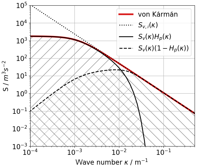
Figure 3Theoretical spectrum for atmospheric turbulence and the contributing filtered spectra as measured by a lidar. The hatched areas show the areas for the integration to calculate (area with forward-slanting lines, “/”) and (area with backward-slanting lines, “\”), whereas the integration of the area under the red curve yields . The dotted line shows the slope of in the inertial subrange.
A generic spectrum, subdivided into areas of lidar-measured variances, appears in Fig. 3. It illustrates the energy that is measured by the lidar LOS measurements by the solid line and the energy that is measured through the turbulent broadening of the spectra by the dashed line. The corresponding variances are the integral of the hatched areas.
Substituting Sv for the von Kármán model (Eq. 8), we obtain
In the inertial subrange of turbulence, the van Kármán model can be simplified to
and in combination with Eq. (6) it can be solved for :
Substituting in Eq. (22) with Eq. (24) results in
With the simplified equation for a Gaussian-shaped filter function Hp,
and substitution of κ for ξ=2πΔzκ, the equation can be rewritten as a function of Δz and Lv:
Substituting ε in Eq. (27) with the solution for ε from Eq. (24), the equation for as a function of Δz and integral length scale Lv, as they appear in Smalikho et al. (2005), can be formulated:
The only unknown is Lv. A downhill simplex algorithm is used to minimize Eq. (28) for Lv
Minimization of Eq. (31) is computationally expensive. To accelerate the data processing, a power function can be defined which approximates the relationship between Lv and :
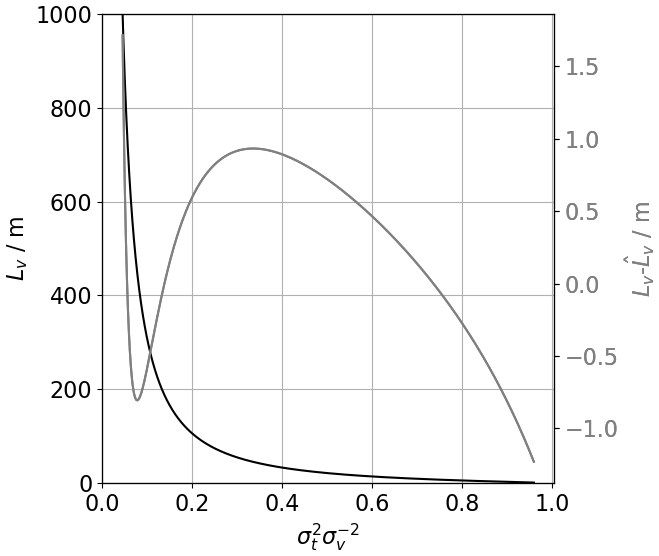
The coefficients c1, c2, and c3 are determined by a curve fit over the range of Lv=3 to 1000 m to Eq. (28). The coefficients are specific for each lidar, since they depend on Δz, and will be determined in Sect. 4. The fitting curve and residuals as obtained through minimization of Eq. (31) appear in Fig. 4. It shows that the error, , that is made with the power-law approximation is in the range of ±1 m. For simplicity, we will use the variable name Lv for integral length scales calculated with Eq. (32) in the following.
With Lv and measured variance in Eq. (24), TKE dissipation rate for the RHI measurements εr can finally be calculated as
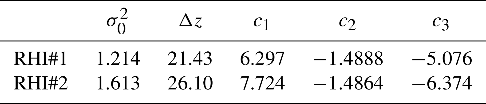
For optimal accuracy of the dissipation rate retrieval, the two unknowns, σ0 and Δz, need to be calibrated according to reference instruments. In this study, the sonic anemometer at 100 m on tower 25/trSE_09 is the closest in situ observation to the RHI scans in the valley. It is used for the calibration by minimizing the root mean square error between this measurement and the respective RHI scan. The resulting parameters differ slightly for lidars RHI#1 and RHI#2 and appear in Table 2 along with the coefficients for the power-law fit of Lv. The difference between Δz and σ0 can be partially attributed to instrumental variability but will also incorporate other sources of error in the turbulence model and data retrieval.
Table 2Adjusted parameters for dissipation rate retrieval from RHI scans.
3.3 Estimation of uncertainties
3.3.1 Sonic anemometers and TLS
To estimate the uncertainty in the retrievals of εs, we apply the law of combination of errors, which describes how random errors propagate through a series of calculations (Barlow, 1989). For a function g=g(xi), with xi being the independent and uncorrelated variables, the law of combination of errors states that, for small errors (i.e. if we ignore 2nd order and higher terms), the variance in the function g, approximated by the sample variance , is given by
where values are the sample variances in the xi values. By applying this method to Eq. (5), the fractional standard deviation in the ε estimate is the following (Piper, 2001):
where I is the sample mean of and is its sample variance.
Similarly, uncertainties are calculated for the TLS measurements εt. However, since the determination of dissipation rate is done in the frequency domain, I in this case is the sample mean of κ5∕3S(κ).
3.3.2 Profiling lidar
The uncertainty in the εv retrievals from the profiling lidars can be estimated from the uncertainty in the LOS velocity variance by also applying the law of combination of errors (Eq. 34) to Eq. (11):
where σσ, v is the uncertainty in the sample variance. This value is not known but is considered to be on the same order of magnitude as the instrument noise and thus set to the value of σe.
3.3.3 RHI
The uncertainty in εr can be calculated by Gaussian uncertainty propagation through Eq. (33) if the uncertainties of the estimation of the integral length scale and the uncertainty in the measurement of the wind speed variance σσ, v are known:
The uncertainty in the variance in radial velocities σσ, v can be determined from the uncertainty in the turbulent broadening estimation σσ, t and the uncertainty in measured LOS velocities :
The uncertainty in the measurement of the integral length scale Lv cannot be determined directly from Eq. (31). A propagation of uncertainties is not possible here, because the function is not differentiable. The approximated function Eq. (32) can, however, be differentiated with respect to σv and σt and can thus be used to propagate uncertainties of the measured values to Lv so that
with c1, c2, and c3 given from Table 2. The uncertainties that are found through this approach are then fed into Eq. (38) in order to calculate the uncertainty in εr.
As can be seen from Eq. (38), the uncertainty in the retrieval of εr depends strongly on the combination of σv and σt. A two-dimensional map visualizing the relative error appears in Fig. 5. The contour lines show that uncertainties grow very large for dissipation rates smaller than 10−3 m2 s−3. Uncertainties are also large for values in excess of 10−1 m2 s−3 if is small at the same time. The input uncertainty σσ, v depends on the CNR and is assumed to be on the order of the corresponding instrumental noise σe. The values in Fig. 5 are calculated with input uncertainties m s−1, which correspond to a CNR value of approximately −12 dB, which is common for the signal strength during the Perdigão campaign for the DLR lidars.
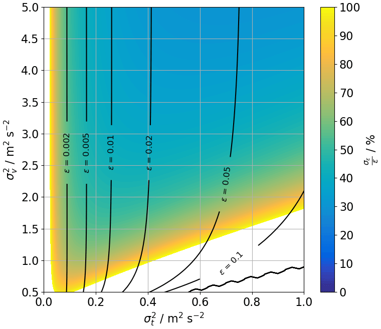
Figure 5Uncertainty estimation for dissipation rate εr depending on measured variances and . The contour lines show the associated εr.
Here we demonstrate a single-point comparison between in situ and remote-sensing retrievals of TKE dissipation rate, and we then compare the remote-sensing estimates of vertical profiles.
4.1 Single-point validation
Sonic anemometer measurements of dissipation rate are continuously available throughout the campaign. The location of tower 25/trSE_09 is approximately 150 m up the valley from the RHI plane and ∼250 m up the valley from the CLAMPS site, where the vertical stare and TLS measurements are taken (Fig. 1). Although small-scale effects can cause significant differences at this distance, we expect a similar diurnal development of turbulence at 100 m above ground from all the instruments considering that they are all within the center of the valley.
Lidars RHI#1 and RHI#2 operated with the same parameters from 9 to 15 June 2017. On some of the days, the RHI measurements were, however, interrupted by other scanning strategies for a few hours. Figure 6 gives a time series of all available estimations of the integral length scale Lv and dissipation rate ε from sonic anemometer and RHI scans for this whole period. As a quality control, all estimates with uncertainty values larger than the actual values are removed as well as all integral length scale values of Lv>2000 m. The diurnal trends compare well between the instruments, but especially for Lv large variations on short timescales are found in both methods. In contrast, dissipation rate shows a better agreement even on the short timescales.
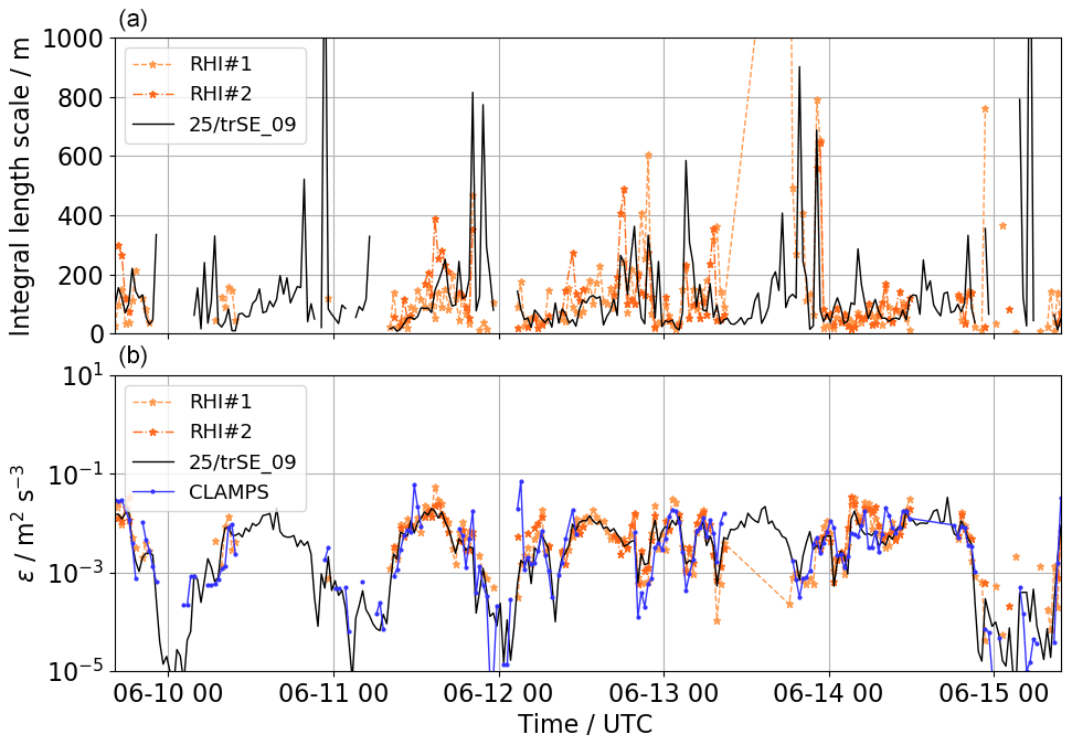
Figure 6Comparison of time series of Lv (a) and ε (b) for the period form 9 to 15 June 2017 for the two RHI lidars RHI#1 and RHI#2 and the sonic anemometer at 100 m on tower 25/trSE_09 in the valley. Estimates for the sonic anemometer are calculated for horizontal wind speed.
Figure 7a shows a scatter plot of ε estimates of the same dataset. Within the observed period, 146 estimates for RHI#1 and 89 estimates for RHI#2 could be retrieved. The difference occurs due to the CNR of the lidar measurement at the location which is compared to the sonic anemometer. A lower CNR is more likely to be filtered. RHI#2 is situated rather close to the tower (∼120 m). With the far focus setting of the lidars (∼1000 m), the CNR at this point is significantly lower for RHI#2 compared to RHI#1 with a distance of ∼500 m to the tower, and thus more data in low-signal conditions are filtered. Since the sonic anemometer has been used for calibration of the RHI retrieval, no biases between the measurements can occur. The correlation between the measurements of R=0.78 can be considered good, given the complex flows and spatial separation between the measurements.
Vertical stare measurements from CLAMPS are available from 6 May through 15 June 2017. With over 1400 half-hour averaged dissipation rate estimates that can be compared with the measurements from the sonic anemometer, this is the largest database used in this study. Figure 6b gives the time series of ε estimates from CLAMPS in the reduced time period from 9–15 June. The results of the whole period are compared in the scatter plot in Fig. 7b. To compare data at the same height, the lidar results have been linearly interpolated to 100 m above ground. The sonic anemometer and CLAMPS vertical stare measurements correlate with a coefficient of R=0.81, with some scatter, which can likely be attributed to the spatial separation between the two instruments and the heterogeneity of complex terrain flow.
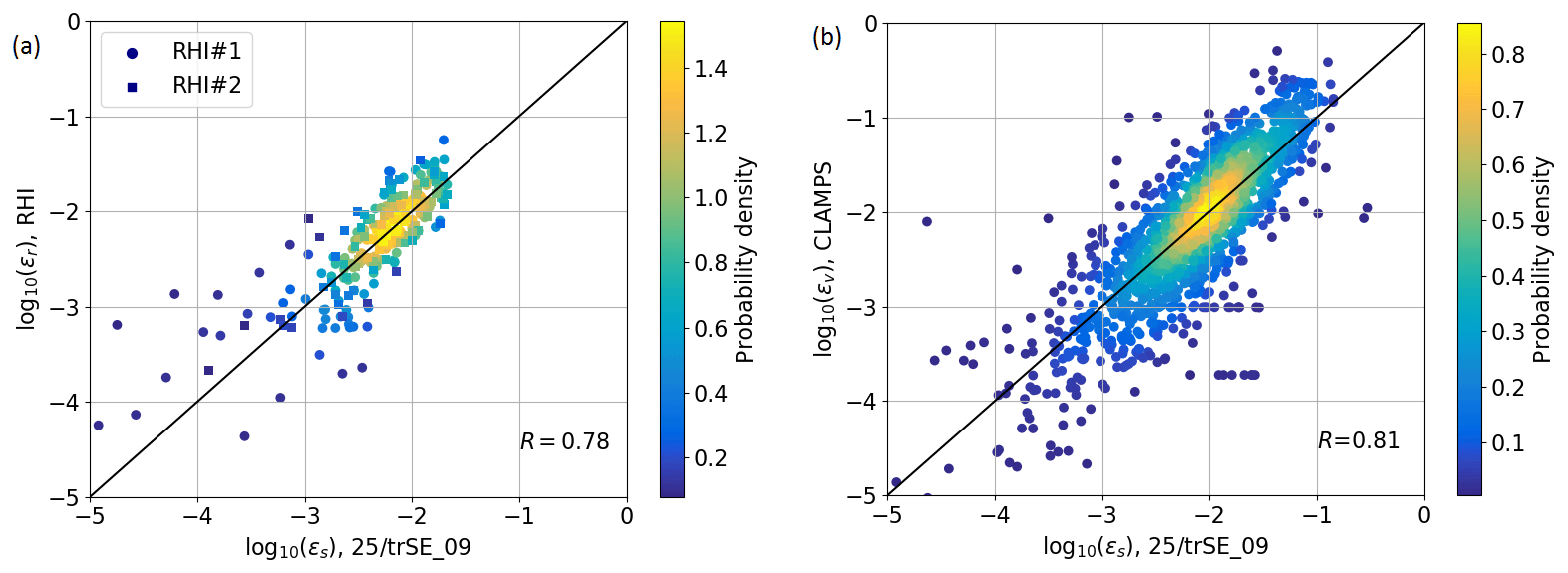
Figure 7Comparison of half-hour averaged estimates of ε at 100 m above ground between the sonic anemometer on tower 25/trSE_09 and the RHI measurements (a) and for the same sonic anemometer and CLAMPS (b). The color scales represent the density of probability of a measurement point. The black line is the line of identity.
For sonic anemometers, TLS and CLAMPS, which are the systems that resolve parts of the inertial subrange of turbulence, the variance spectra appear in Fig. C1 in Appendix C.
4.2 Comparison of lidar retrievals
To systematically quantify the agreement between RHI and vertical stare retrievals of dissipation rate, all valid measurement points between −150 and 800 m above ridge height at the location, where the vertical stare measurements are taken, can be compared for the period from 9–15 June 2017. For this purpose, the values of both systems are linearly interpolated to the same heights and compared (Fig. 8). Unfortunately, in this time period the CLAMPS lidar was shut off due to overheating during most of the days as can be seen in Fig. 6. Thus, most of the dataset for this comparison contains nighttime data. Despite this, a reasonable correlation is found (R=0.61 for RHI#1 and R=0.68 for RHI#2), with a larger scatter especially for values of ε less than 10−3 m2 s−3.
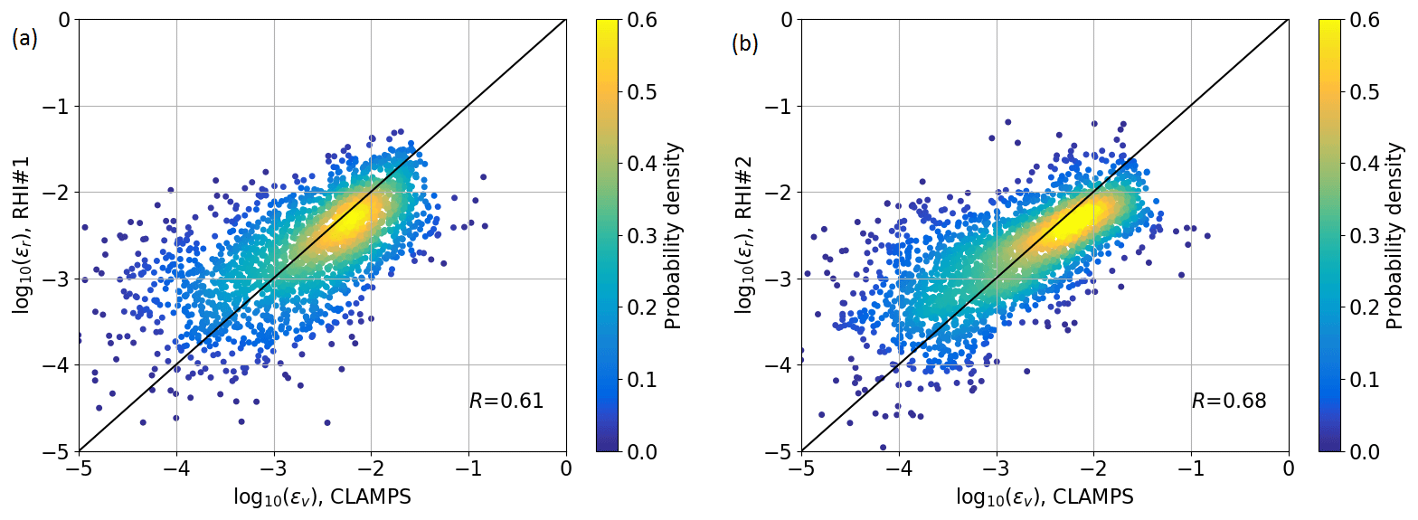
Figure 8Comparison of all estimates of ε in the vertical profile over the valley from 9 to 15 June 2017 from RHI#1 (a) and RHI#2 (b) against the Halo Photonics system. The color scale represent the density of probability of a measurement point. The black line shows the identity line.
If the theory of local isotropy in the small scales of turbulence holds, estimates of εr should not depend on the direction of the lidar beams. The elevation angles at the same points in space differ significantly for the two lidars over the whole RHI plane. A comparison between retrievals of εr from the two lidars performing RHI scans in the whole observed area for the period from 9 to 15 June (Fig. 9) shows a very good agreement between 10−3 and 10−1 m2 s−3. Again, a rather large scatter occurs in the region of low turbulence. Outliers with a probability density of less than 0.02 have been removed from Fig. 9. These are mostly due to hard-target reflections that can occur at any point in space, e.g., due to clouds, and were not filtered in all cases.
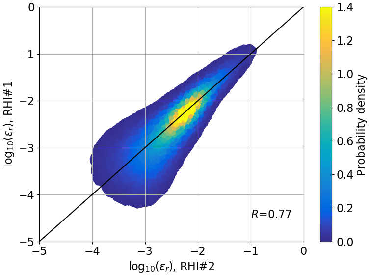
Figure 9Comparison of all estimates of ε in the RHI plane for 9–15 June 2017 between RHI#1 and RHI#2. The color scales represent the probability of occurrence of a measurement point. The black line is the line of identity. Data points with probability density below 0.02 are not shown.
5.1 Comparison of dissipation rate estimates in a nighttime LLJ
Between 13 June, 21:00 UTC, and 14 June, 12:00 UTC, data are available from all the stationary instruments, and the TLS made multiple successive ascents and descents. During this night, a low-level jet (LLJ) from the southwest occurred, with its peak wind speed at varying heights between 200 and 400 m above ridge height, inducing shear and veer within and above the valley. An example of the two-dimensional wind field over the valley, as reconstructed from the RHI scans of lidars RHI#1 and RHI#2 (Wildmann et al., 2018a), for an averaging period of 30 min, appears in Fig. 10a. Figure 10b and c show corresponding vertical profiles of the vertical stare estimate εv and TLS estimate εt on top of the two-dimensional retrieval of εr from RHI#1 and RHI#2. The larger turbulence in the shear layers at the upper and lower bound of the LLJ emerge clearly in this representation. Missing data points occur in the very low turbulence regions in the center of the jet and above 600 m above the ridge top. At these points, the Doppler spectral width becomes too small to be distinguished from noise, i.e. the value of E in Eq. (14) is not negligible any more. Appendix B and the Supplement present a description of the atmospheric conditions for this LLJ event.
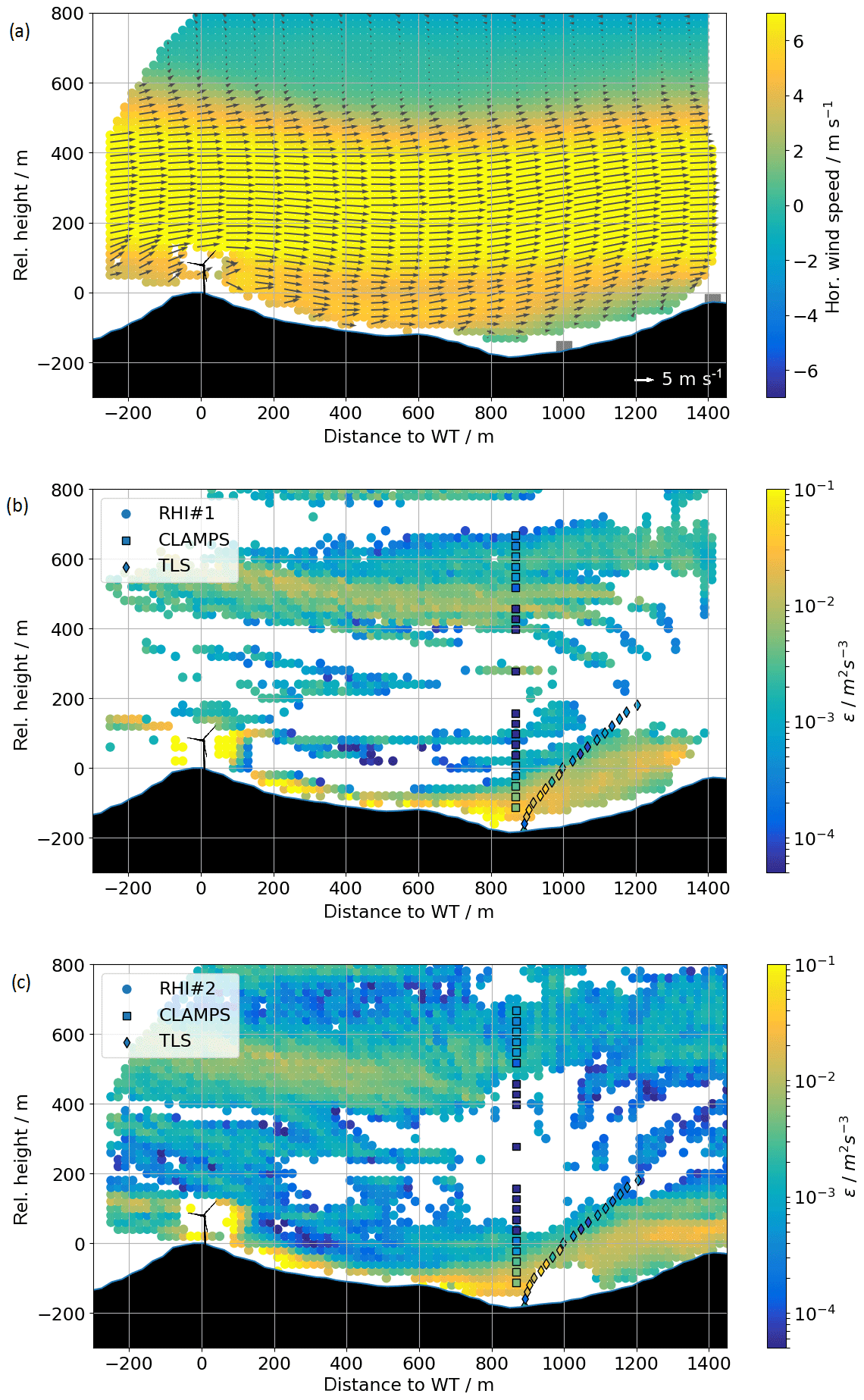
Figure 10In panel (a) the coplanar wind field reconstruction from RHI#1 and RHI#2 from averaged RHI scans between 04:00 and 04:30 UTC is shown. The arrows show the wind vectors projected onto the RHI plane as retrieved with the coplanar method (Wildmann et al., 2018a). The color map is scaled with the horizontal wind component of the projected wind vector. Panels (b, c) show dissipation rates as estimated from vertical stare and TLS on RHI scans by RHI#1 (b) and RHI#2 (c) for the same time period. The origin of the local coordinate system in this and all the following plots is at the wind turbine base location on the SW ridge.
To investigate the vertical structure of turbulence in the presence of the LLJ more closely, we assess profiles of TKE dissipation rate. Both TLS and lidars allow for collection of estimates throughout the whole ABL. Therefore, the TLS and the lidars enable estimates of turbulence from the network of sonic anemometers to extend to higher altitudes. Vertical profiles of TKE dissipation rate can then be measured both in and over the valley, which is particularly important when assessing turbulence in nighttime LLJ flows. The average vertical profiles of ε as measured by the CLAMPS vertical stare measurements, the RHIs, and the TLS for two selected time periods (04:00–04:30 and 05:00–05:30 UTC) appear in Fig. 11. The RHI profiles are extracted from the two-dimensional fields at that horizontal distance to the WT, which is given for the CLAMPS vertical stare measurements. The sonic anemometer measurements at all levels on towers 20/trSE_04 and 25/trSE_09 are also included in the profiles. Data from the lidars and the sonic measurements represent half-hour averages, whereas the TLS measurements are quasi-instantaneous, with a moving spatial filter of approximately 20 m for the ascents and descents at constant speed. Since the collection of a full profile at an ascent of 0.3 m s−1 lasts approximately 23 min, these high-resolution measurements suggest some idea about the variability in ε within the averaging period of the other systems. The gap in the measurements between 200 and 400 m above the ridge-top height is due to low turbulence in that region which could not be adequately sampled with the lidars. The upper limit of TLS measurements was limited by flight permissions. All instruments indicate a large gradient of turbulence at ridge height, with values of ε at 100 m above the ridge almost 2 orders of magnitude smaller than in the valley. At 04:00–04:30 UTC, a large variability among the different platforms occurs, when the LLJ is still well defined, with maximum wind speed at 300 m above ridge height. One hour later, with a LLJ that is broadening and weakening, the vertical profiles of all systems agree better above the ridge. Moreover, as also seen in Fig. 12, all valley instruments measure increased turbulence in the valley except for the sonic anemometers from 05:00 to 05:30 UTC.
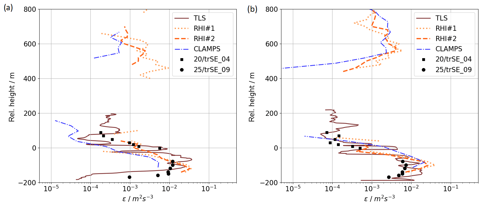
Figure 11Comparison of average vertical profiles of eddy dissipation rate ε measured by lidar vertical stare, RHI scans, TLS, and sonic anemometers on meteorological towers at 04:00–04:30 UTC (a) and at 05:00–05:30 UTC (b).
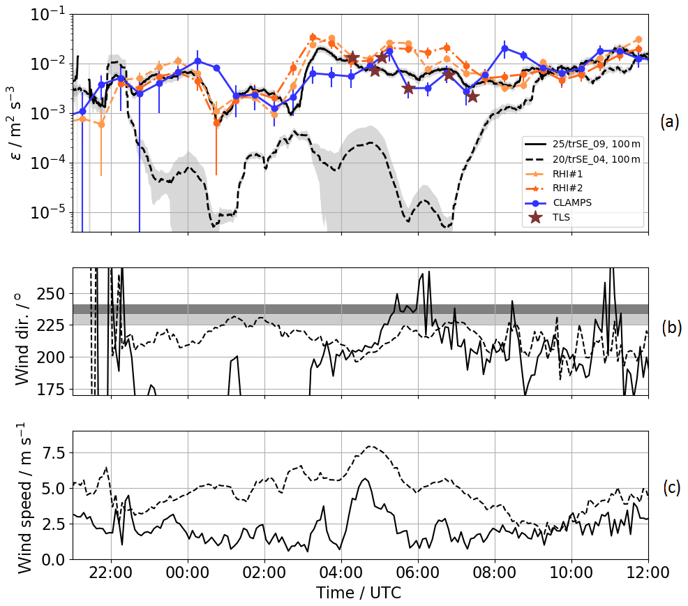
Figure 12Comparison of ε as measured by the RHI scans, the vertical stare measurements, the TLS, and two reference sonic anemometers from 13 to 14 June 2017, 21:00–12:00 UTC (a). Panel (b) shows the wind direction and panel (c) the wind speed measured by sonic anemometers at the 100 m level over the ridge and in the valley. The shaded areas in (b) give the wind direction regions in which CLAMPS (light gray) and RHI#1 and #2 (dark gray) are in the line of sight of the WT rotor plane.
Looking at a time series of the TKE dissipation rates in the valley at a height corresponding to the 100 m sonic anemometer on tower 25/trSE_09 gives more insight into the development of turbulence in the valley throughout the night (Fig. 12). Dissipation rate from the TLS is calculated for a time series corresponding to a height bin between 90 and 110 m above ground during its ascents and descents to facilitate comparison with the 100 m tower measurements. While different instruments within the valley generally concur within their uncertainty bands, tower 20/trSE_04 on the ridge suggests very different (and smaller) values of dissipation. The best agreement emerges between the TLS and CLAMPS, which both measure approximately at the same location. In some periods, CLAMPS estimates deviate from the other systems, which can potentially be attributed to specific wind directions and local turbulence features. The comparison between the two towers on the ridge and in the valley shows that during the night the turbulence in the valley is decoupled from the flow above ridge height, while 1 h after sunrise, which is at 06:01 UTC, the retrieved values of ε converge. Similarly, wind speed values (Fig. 12c) between the ridge and valley also differ through the night until convergence after sunrise.
5.2 Wind turbine wake turbulence
A systematic difference in dissipation rate estimates between instruments in different locations can be found between 04:30 and 07:00 UTC (Fig. 12a). Here we present evidence that this disagreement arises because of spatial heterogeneity in turbulence related to the propagation of the wind turbine wake within the measurement domain.
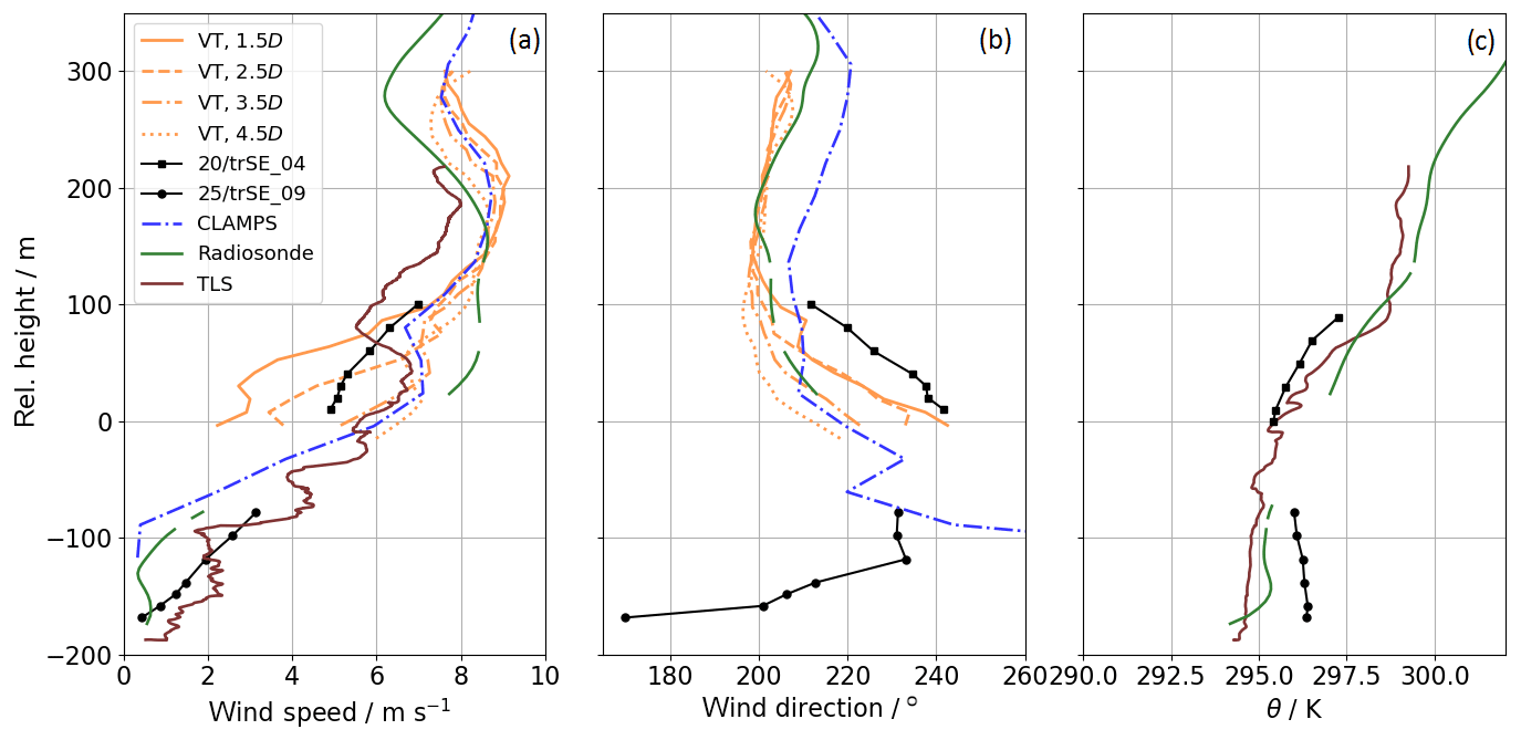
Figure 13Vertical profiles of wind speed (a), wind direction (b), and potential temperature θ (c) from 05:00 to 05:30 UTC. For wind speed, tower data of towers 20/trSE_04 and 25/trSE_09 are complemented with profiles of the virtual towers (VTs). For θ, TLS measurements are included.
During this specific time period, wind speeds at the SW ridge (tower 20/trSE_04, Fig. 12c) exceeded 5 m s−1, which is well within the power-production range of the WT, and generation of a wind turbine wake can be expected. From Fig. 12b we can see that the local wind direction steers the wake toward the measurement volumes of the instruments discussed here: into the region measured by the CLAMPS and TLS between 05:00 and 05:30 UTC and into the RHI plane after 05:30 UTC.
From 05:00 to 05:30 UTC, vertical profiles of wind speed, wind direction, and potential temperature as observed by multiple instruments provide insight into the steering of the wake (Fig. 13). In addition to the TLS, a radiosonde, the tower 25/trSE_09, and the CLAMPS VAD measurements, which are all located in the valley center, Fig. 13, also include data from tower 20/trSE_04 on the SW ridge next to the turbine, as well as half-hour averages of virtual towers (VTs) calculated at the intersection lines of the RHIs of all three DLR lidars, including RHI#3 (for details about the VT method, see Bell et al., 2019). The VTs provide a wind estimate downwind of the wind turbine, at four distinct locations, each separated by one rotor diameter, D=82 m (as highlighted in Fig. 1). The vertical profiles of wind direction from the four VTs match each other down to a height of 100 m above ridge height. Below this, winds veer with different strength, depending on the location on the sloping valley transect. At the 100 m level of tower 25/trSE_09 (within the valley), a wind direction of 225∘ is measured aligning the wind turbine with the CLAMPS site. Potential temperature measurements by the radiosonde that was released at 05:16 UTC in the valley and by the TLS clearly show a remaining nighttime inversion capping the boundary-layer flow approximately 100 m above ridge height.
Between 05:30 and 06:00 UTC, turbulence retrievals from the RHI measurements (Fig. 12) suggest large turbulence levels in the valley, whereas the rest of the instruments observe significantly lower turbulence. This corresponds to a wind direction in the valley that has veered further towards the RHI plane in a wind direction of 235∘. At the same time, the coplanar wind retrievals in the RHI plane show a wind turbine wake with clearly detectable wind speed deficit (Fig. 14) in the first 250 m near the turbine. Further downstream, wind speed deficits of the wake are hard to distinguish from the ambient flow. Numerous previous observations (Bodini et al., 2017) and simulations (Vollmer et al., 2017; Englberger et al., 2019) indicate that wakes veer in response to ambient veer.
The 2-D plots of εr by RHI#1 and RHI#2 (Fig. 14) support the theory of wake-induced turbulence propagating into the valley with the mean flow by showing constantly large turbulence between WT and the valley and even some indication of the expected tip vortex turbulence in the WT near field.
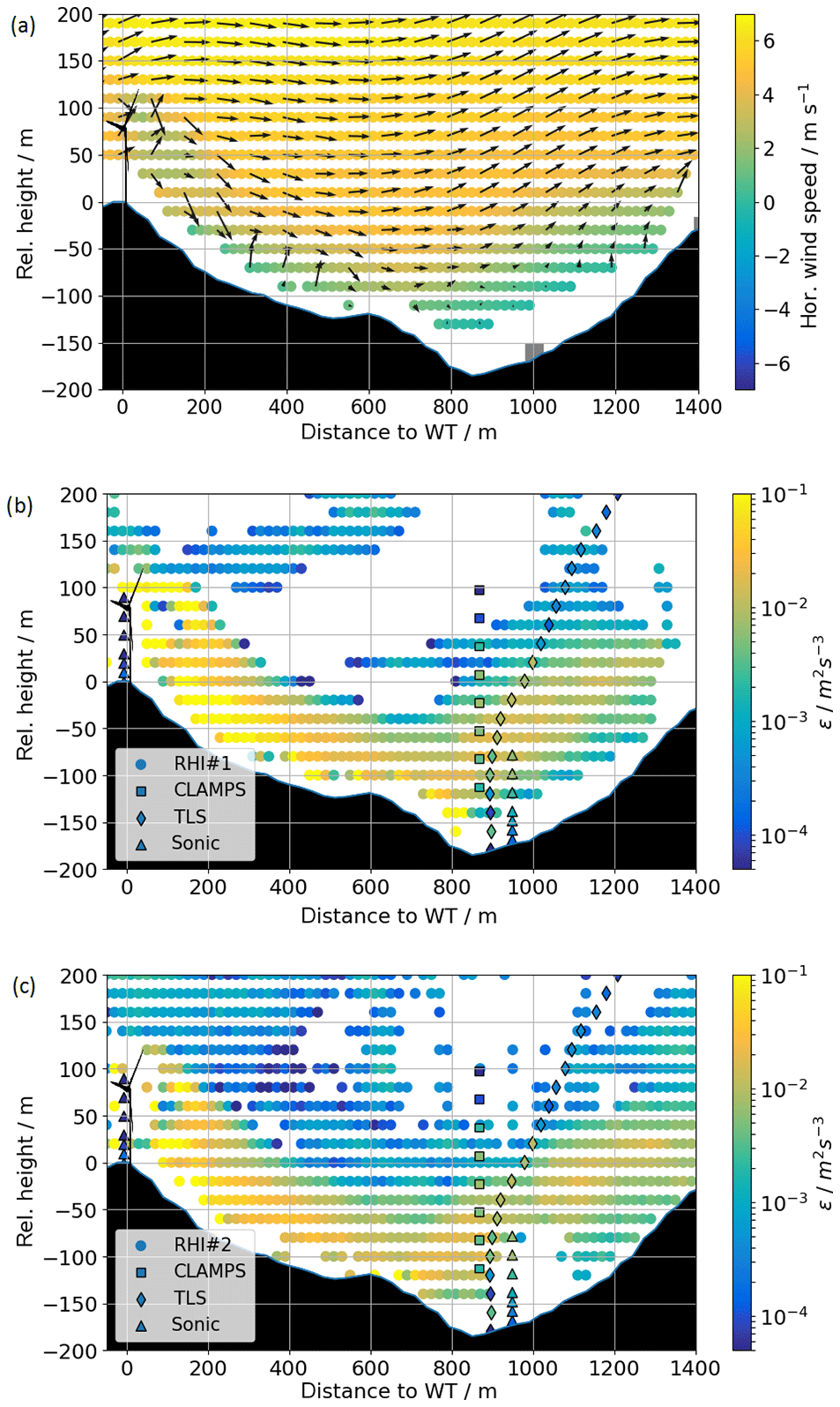
Figure 14In panel (a) the coplanar wind field reconstruction from RHI#1 and RHI#2 from averaged RHI scans between 05:30 and 06:00 UTC is shown. The arrows show the wind vectors projected onto the RHI plane as retrieved with the coplanar method (Wildmann et al., 2018a). The color map is scaled with the horizontal wind component of the projected wind vector. Panels (b, c) show dissipation rates as estimated from CLAMPS, TLS, and towers 20/trSE_04 and 25/trSE_09 on scans by RHI#1 (b) and RHI#2 (c) for the same time period.
The dissipation rate measured in the waked region by the lidar systems more than 10 rotor diameters downstream of the WT is approximately m2 s−3, compared to m2 s−3 measured by the sonic anemometer in the region less effected by the wake-induced turbulence. These differences are smaller than 2 orders of magnitude within-wake differences and out-of-wake differences by Lundquist and Bariteau (2015), but the Perdigão measurements are much further downwind than the Lundquist and Bariteau (2015) measurements. Also, with the veering wind and the available data, we cannot say at which lateral position in the wake the measurements are taken and what are the maximum turbulence levels in the wake.
6.1 Turbulence measurement in a complex terrain
This study demonstrates how measurements of multiple instruments can be synthesized to evaluate the spatiotemporal evolution of turbulence in a highly complex terrain. Vertical profiles retrieved from vertical stare measurements of a scanning lidar compare well with in situ measurements from meteorological masts and a TLS, extending the upper limit of the vertical profile significantly. The new retrieval method for TKE dissipation rate from RHI scans allows for localization of the origin of turbulence in a way that would not be possible with point measurements or vertical profiles alone. This approach enables insights into the variability of turbulence in a complex terrain. Some remarks have to be made on the turbulence retrievals with Doppler lidars:
-
The uncertainty in the measurement of LOS variance depends on the signal strength of the atmospheric backscatter. While the atmospheric conditions were sufficient for the data presented here, the availability of lidar measurements is limited in conditions of very low aerosol in the ABL, rain, or fog. Very high temperatures can demand a shut-off of the lidars as it was the case for the CLAMPS lidar during daytime from 9 to 15 June 2017.
-
An averaging of measured LOS velocity along the lidar beam is inherent to the Doppler lidar technology. The size of this averaging volume defines the limits of detectable eddies in the LOS velocities. For the systems used in this study, the width of this averaging window is on the order of a few tens of meters. For integral length scales, Lv, smaller than this averaging window, the assumptions that are used in the theory described in Sect. 3 will be violated. For the RHI method, σt will not contain scales within the inertial subrange exclusively, and for the vertical stare method measured spectra will differ significantly from the model spectra.
-
The analytic uncertainty estimation and the comparison to a sonic anemometer both show that the dissipation rates below 10−4 m2 s−3 cannot be resolved appropriately with the presented methods. Measurements below 10−3 m2 s−3 are already subject to high uncertainties.
Given these limitations, we still see that lidar measurements reliably detect time periods and spatial regions of increased turbulence.
Regarding the method of turbulence retrieval from RHI measurements, we find the following:
-
A careful calibration of and Δz with respect to reference instruments is necessary in order to obtain reliable results for TKE dissipation rate.
-
While storing raw Doppler spectrum data of the wind lidars may seem expensive in a field campaign, these data enable averaging multiple measurements in the spectral domain and thus increasing the signal-to-noise ratio. Whenever possible, these raw spectra should be saved from field campaigns with an interest in turbulence variability.
Given numerous logistical constraints, the lidars, sonic anemometers, and TLS in this experiment could not collect measurements at the same location. Given the complex terrain, a difference in measurement location of only a few hundred meters can cause significant differences in the observations of the flow field and its turbulence. This spatial heterogeneity should be considered in the evaluation of the magnitude of correlation between the instruments. Previous studies evaluating profiling lidars with the same retrieval methods as presented in this study in a flat terrain yield similar correlation coefficients with sonic anemometer measurements (R=0.84; Bodini et al., 2018) but without the filtering of bad fits to the spectral model. The lowest correlation is found between CLAMPS and the RHI methods, which is likely because of the dataset for this comparison, which contains mostly measurements at nighttime and low-turbulence conditions within the most limited time frame. We showed in Sect. 3.3 that the low-turbulence conditions are those of highest uncertainties. For future campaigns in complex terrains, co-located in situ instruments in the measurement volume of the lidar are recommended to decrease the influence of spatial variability and improve the possibilities to validate lidar turbulence retrievals.
6.2 Wind turbine wakes in complex terrains
Menke et al. (2018) and Wildmann et al. (2018a) showed that wind turbine wakes in stable stratification at the Perdigão campaign can be observed far downstream, following the terrain into the valley of Vale do Cobrão. By means of wake-tracking algorithms based on the wind speed deficit, the wake could be detected up to 10 rotor diameters downstream in very stable atmospheric conditions. From the RHI measurements shown in Fig. 14, increased turbulence is observed in the near field of the WT and at least three rotor diameters downstream. To be able to distinguish wake-induced turbulence from the background turbulence further downstream in the valley, it was necessary to include other observations of turbulence as well as information about wind speed, wind direction, and potential temperature. Only the aggregate of all observations provides strong evidence that the wake of the wind turbine in the night of 14 June is advected and stretched with the mean wind into the valley. Small wind-direction changes cause large changes in observed turbulence at the specific instrument locations, which suggests that even at 11D downstream the wind turbine wake is a local feature which is not completely eroded in the background turbulence. These data cannot quantify how much the background turbulence is affected by the wake or how turbulent mixing in the valley is enhanced by the presence of the wake. Extending the dataset to more cases during the Perdigão campaign and a comparison to measurements at other locations and campaigns is necessary for conclusive analyses towards these goals.
We employ several instruments and analysis methods to provide a comprehensive view of turbulence structures and variability at the Perdigão 2017 field campaign. We quantify turbulence dissipation rate using vertically profiling lidars and a new analysis method using RHI lidar scans. These remote-sensing methods compare well to in situ methods, using sonic anemometers on meteorological towers or hot-wire anemometers mounted on a tethered lifting system. We also offer means to quantify the uncertainty in dissipation rate estimates. For one case study, we find brief periods of disagreement between the methods, but we can attribute that disagreement to the propagation and meandering of a wind turbine wake which does not affect all measurements simultaneously.
This study gives a good example of the multitude and variety of methods and instruments that are available and beneficial to sample the complex flow in mountainous terrain. Within its limitations, lidar remote sensing is a powerful tool to sample wind and turbulence and provide spatiotemporal data which can be directly compared to numerical models. Utilizing the methods introduced in this study, more measurements by at least eight other lidar instruments performing RHI scans at the Perdigão 2017 campaign could be analyzed in future to expand the analysis of spatial distribution of turbulence and thus provide a unique dataset for validation of numerical models in a complex terrain.
A remaining challenge is the adequate sampling of very low turbulence in the stable ABL, which cannot easily be improved with the current state-of-the-art lidar technology. A different kind of lidar system or other measurement technology is necessary in these cases. Remotely piloted aircraft (RPA) are increasingly used in stable ABL research (Kral et al., 2018) as well as for investigations in complex terrains (Wildmann et al., 2017). As such, they are a promising tool to validate and complement remote-sensing data in similar ways as shown in this study.
The physics of WT wakes remains an important field of research for wind farm design and control. Providing spatial information of wind and turbulence with lidar data is already and will still be of great importance for future research in the field. The methods presented in this study can therefore not only provide valuable information about turbulence in complex terrains but also about turbulence in the wake of wind farms including offshore sites where wake effects can have a large impact on the mixing of the ABL in specific atmospheric conditions as observed in measurements (Platis et al., 2017) and mesoscale simulations (Siedersleben et al., 2018).
High-rate data from sonic anemometers on the meteorological masts (UCAR/NCAR, 2019) and quality-controlled radiosonde data (UCAR/NCAR, 2018) as well as CLAMPS lidar data (Klein and Bell, 2017) are available through the Earth Observing Laboratory project website at https://www.eol.ucar.edu/field_projects/perdigao (last access: 18 November 2019). DLR lidar data are available through https://perdigao.fe.up.pt/ (re3data.org, 2019).
| ε | TKE dissipation rate |
| εr | dissipation rate estimations from lidar RHI |
| εs | dissipation rate derived from sonic anemometer measurements |
| εt | dissipation rate derived from TLS measurements |
| εv | dissipation rate estimations from lidar vertical stare |
| σε, s | uncertainty in dissipation rate estimations by sonic anemometers |
| σε, t | uncertainty in dissipation rate estimations by TLS |
| σε, v | uncertainty in dissipation rate estimations by vertical stare lidar |
| σε, r | uncertainty in dissipation rate estimations by RHI lidar |
| σσ, v | uncertainty in LOS velocity variance |
| σσ, t | uncertainty in turbulent broadening |
| uncertainty in lidar LOS velocity variance measurement | |
| Doppler spectral width at zero wind speed | |
| lidar instrumental noise | |
| σp | lidar pulse width |
| lidar-measured shear contribution to variance | |
| lidar-measured Doppler spectral width | |
| turbulent broadening of the Doppler spectrum | |
| velocity variance | |
| lidar-measured LOS velocity variance | |
| sample variance of | |
| σL, v | uncertainty in integral length scale estimation |
| ΔR | distance between neighboring range gate centers |
| Δz | length of the lidar sensing volume |
| lidar-measured LOS velocity | |
| average lidar-measured LOS velocity | |
| Bv | correlation function of flow velocity |
| Ck | Kolmogorov constant |
| Dv | structure function of velocity |
| E | random error in spectral width measurement |
| ES | mean error between measured spectrum and model |
| Hp | low-pass filter function for lidar measurement |
| Lv | integral length scale |
| approximated integral length scale | |
| Qs | lidar sensing volume window function |
| Sv | energy spectrum of flow velocity |
| lidar-measured spectral energy | |
| Tw | lidar time window |
To understand the flow system with a LLJ from the southwest (SW), which occurred in the night from 13 to 14 June 2017, the long-term Weather Research and Forecasting model (WRF) simulation as described in Wagner et al. (2019a) is consulted. The meteorological situation was characterized by a synoptic low-pressure system at 850 hPa, which was located over the Atlantic Ocean SW of the Iberian Peninsula. The combination of synoptic and thermally driven forcings and the interaction with the complex terrain around Perdigão resulted in a highly complex boundary-layer flow. Unlike in most nights during the Perdigão 2017 campaign, a LLJ from SW developed instead of the usual northeasterly LLJ (as it was also observed in the nights before and after this case study). Figure B1 shows profiles of simulated wind speed and wind direction at the location of tower 20/trSE_04 averaged over the time interval between 03:00 and 03:30 UTC on 14 June 2017. In addition, wind speed and wind direction measured by the radiosonde (RS) launched in the valley at 02:55 UTC are shown to verify the simulated wind profile. Note that the RS does not measure a purely vertical profile, as it is drifting horizontally with the wind. Both simulated and observed profiles indicate the strong LLJ from the SW near the surface, a strong directional wind shear above the jet with southerly and even easterly winds at 850 hPa (1.5 km altitude), and increased wind speeds from the SW in the free troposphere with a maximum at 500 hPa. In the Supplement, we provide WRF maps of wind speed at 600 m above sea level, 850 and 500 hPa, and a Hovmöller plot from 11 June through 16 June 2019 to illustrate the synoptic situation during the night of the case study.
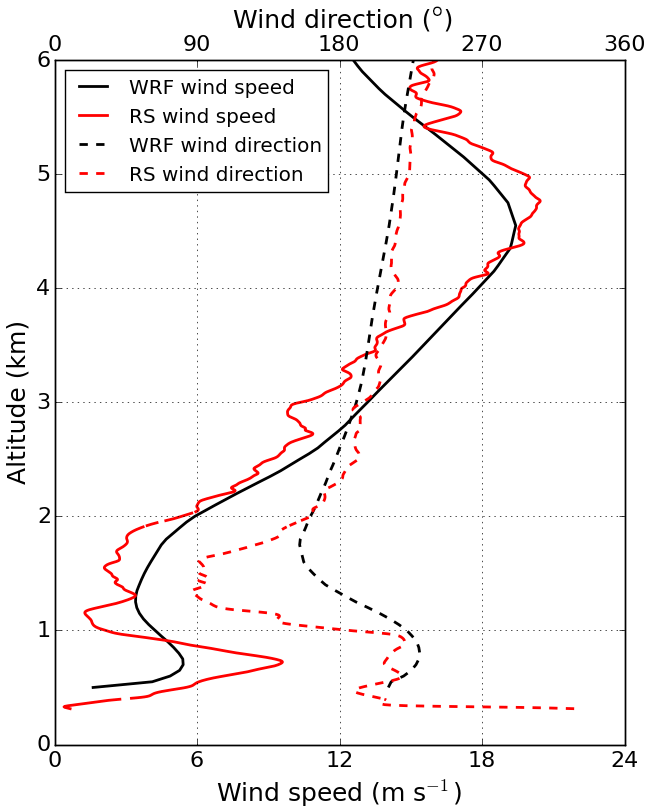
Figure B1Wind speed and wind direction up to 6 km as an average from 03:00 to 03:30 UTC from WRF simulations (black lines) and from the radiosonde (RS, red lines) launched at 02:55 UTC on 14 June 2017.
For sonic anemometer, TLS, and lidar vertical stare measurements, power spectra of measured flow velocity can be calculated and show how these instruments resolve turbulence at different scales. Only a careful choice of the scales that are used to derive ε, as it is done in this study, allows a valid comparison.
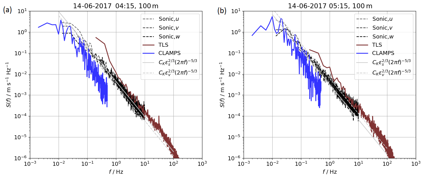
Figure C1Variance spectrum of TLS (between 90 and 110 m above the ground), vertical stare, and sonic anemometer at 100 m above ground for the time period 04:00–04:30 UTC (a) and 05:00–05:30 UTC (b).
The supplement related to this article is available online at: https://doi.org/10.5194/amt-12-6401-2019-supplement.
JKL, LB, NB, and NW helped design and carry out the field measurements. NB analyzed the data from the sonic anemometers and the profiling lidars. LB analyzed the data from the TLS. NW analyzed the data from the RHI lidars and made the figures, in close consultation with JKL, LB, NB, and JW. JW ran the WRF simulations and provided the plots for Appendix B and the Supplement. NW wrote the paper, with significant contributions from JKL and NB. All the coauthors contributed to refining the paper text.
The authors declare that they have no conflict of interest.
We want to thank José Palma, University of Porto, José Carlos Matos, and the INEGI team for the local organization and tireless work in order to make this experiment a success. We acknowledge all the hard work of the DTU and NCAR staff to provide large parts of the hardware and software infrastructure available at Perdigão. We also acknowledge Petra Klein and Tyler Bell for the measurements with the CLAMPS lidar and the provision of data.
We appreciate the hospitality and help we received from the municipality and residents of Alvaiade and Vila Velha de Rodão throughout the campaign.
We want to thank Anton Stephan and Thomas Gerz for internal review of the article and their valuable comments.
This research has been supported by the Federal Ministry of Economy and Energy Germany (grant nos. 0325518 and 0325936A) and the US National Science Foundation (grant nos. AGS-1554055 and AGS-1565498).
The article processing charges for this open-access
publication were covered by a Research
Centre of the Helmholtz Association.
This paper was edited by Laura Bianco and reviewed by Raghavendra Krishnamurthy and one anonymous referee.
Adler, B. and Kalthoff, N.: Multi-scale Transport Processes Observed in the Boundary Layer over a Mountainous Island, Bound.-Lay. Meteorol., 153, 515–537, 2014. a
Balsley, B. B., Frehlich, R. G., Jensen, M. L., Meillier, Y., and Muschinski, A.: Extreme Gradients in the Nocturnal Boundary Layer: Structure, Evolution, and Potential Causes, J. Atmos. Sci., 60, 2496–2508, 2003. a
Barlow, R. J.: Statistics: a guide to the use of statistical methods in the physical sciences, vol. 29, John Wiley & Sons, 1989. a
Belcher, S. E., Harman, I. N., and Finnigan, J. J.: The Wind in the Willows: Flows in Forest Canopies in Complex Terrain, Annu. Rev. Fluid Mech., 44, 479–504, https://doi.org/10.1146/annurev-fluid-120710-101036, 2012. a
Bell, T., Klein, P., Wildmann, N., and Menke, R.: Analysis of Flow in Complex Terrain Using Multi-Doppler Lidar Retrievals, Atmos. Meas. Tech. Discuss., https://doi.org/10.5194/amt-2018-417, in review, 2019. a
Beyrich, F., Leps, J.-P., Mauder, M., Bange, J., Foken, T., Huneke, S., Lohse, H., Lüdi, A., Meijninger, W., Mironov, D., Weisensee, U., and Zittel, P.: Area-Averaged Surface Fluxes Over the Litfass Region Based on Eddy-Covariance Measurements, Bound.-Lay. Meteorol., 121, 33–65, 2006. a
Bodini, N., Zardi, D., and Lundquist, J. K.: Three-dimensional structure of wind turbine wakes as measured by scanning lidar, Atmos. Meas. Tech., 10, 2881–2896, https://doi.org/10.5194/amt-10-2881-2017, 2017. a
Bodini, N., Lundquist, J. K., and Newsom, R. K.: Estimation of turbulence dissipation rate and its variability from sonic anemometer and wind Doppler lidar during the XPIA field campaign, Atmos. Meas. Tech., 11, 4291–4308, https://doi.org/10.5194/amt-11-4291-2018, 2018. a, b, c, d, e
Bodini, N., Lundquist, J. K., Krishnamurthy, R., Pekour, M., Berg, L. K., and Choukulkar, A.: Spatial and temporal variability of turbulence dissipation rate in complex terrain, Atmos. Chem. Phys., 19, 4367–4382, https://doi.org/10.5194/acp-19-4367-2019, 2019. a
Bonin, T. A., Choukulkar, A., Brewer, W. A., Sandberg, S. P., Weickmann, A. M., Pichugina, Y. L., Banta, R. M., Oncley, S. P., and Wolfe, D. E.: Evaluation of turbulence measurement techniques from a single Doppler lidar, Atmos. Meas. Tech., 10, 3021–3039, https://doi.org/10.5194/amt-10-3021-2017, 2017. a, b
Champagne, F. H.: The fine-scale structure of the turbulent velocity field, J. Fluid Mech., 86, 67–108, https://doi.org/10.1017/S0022112078001019, 1978. a
Dupont, S. and Brunet, Y.: Coherent structures in canopy edge flow: a large-eddy simulation study, J. Fluid Mech., 630, 93–128, https://doi.org/10.1017/S0022112009006739, 2009. a
Eberhard, W. L., Cupp, R. E., and Healy, K. R.: Doppler Lidar Measurement of Profiles of Turbulence and Momentum Flux, J. Atmos. Ocean. Tech., 6, 809–819, https://doi.org/10.1175/1520-0426(1989)006<0809:DLMOPO>2.0.CO;2, 1989. a
Englberger, A., Dörnbrack, A., and Lundquist, J. K.: Does the rotational direction of a wind turbine impact the wake in a stably stratified atmospheric boundary layer?, Wind Energ. Sci. Discuss., https://doi.org/10.5194/wes-2019-45, in review, 2019. a
Fairall, C. W., Edson, J. B., Larsen, S. E., and Mestayer, P. G.: Inertial-dissipation air–sea flux measurements: a prototype system using realtime spectral computations, J. Atmos. Ocean. Tech., 7, 425–453, https://doi.org/10.1175/1520-0426(1990)007<0425:IDASFM>2.0.CO;2, 1990. a
Fernando, H. J. S., Mann, J., Palma, J. M. L. M., Lundquist, J. K., Barthelmie, R. J., Belo-Pereira, M., Brown, W. O. J., Chow, F. K., Gerz, T., Hocut, C. M., Klein, P. M., Leo, L. S., Matos, J. C., Oncley, S. P., Pryor, S. C., Bariteau, L., Bell, T. M., Bodini, N., Carney, M. B., Courtney, M. S., Creegan, E. D., Dimitrova, R., Gomes, S., Hagen, M., Hyde, J. O., Kigle, S., Krishnamurthy, R., Lopes, J. C., Mazzaro, L., Neher, J. M. T., Menke, R., Murphy, P., Oswald, L., Otarola-Bustos, S., Pattantyus, A. K., Rodrigues, C. V., Schady, A., Sirin, N., Spuler, S., Svensson, E., Tomaszewski, J., Turner, D. D., van Veen, L., Vasiljević, N., Vassallo, D., Voss, S., Wildmann, N., and Wang, Y.: The Perdigão: Peering into Microscale Details of Mountain Winds, B. Am. Meteorol. Soc., 100, 799–819, https://doi.org/10.1175/BAMS-D-17-0227.1, 2019. a, b
Frehlich, R., Meillier, Y., Jensen, M. L., and Balsley, B.: Turbulence Measurements with the CIRES Tethered Lifting System during CASES-99: Calibration and Spectral Analysis of Temperature and Velocity, J. Atmos. Sci., 60, 2487–2495, https://doi.org/10.1175/1520-0469(2003)060<2487:TMWTCT>2.0.CO;2, 2003. a
Frehlich, R., Meillier, Y., and Jensen, M. L.: Measurements of Boundary Layer Profiles with In Situ Sensors and Doppler Lidar, J. Atmos. Ocean. Tech., 25, 1328–1340, https://doi.org/10.1175/2007JTECHA963.1, 2008. a, b, c
Goger, B., Rotach, M. W., Gohm, A., Fuhrer, O., Stiperski, I., and Holtslag, A. A. M.: The Impact of Three-Dimensional Effects on the Simulation of Turbulence Kinetic Energy in a Major Alpine Valley, Bound.-Lay. Meteorol., 168, 1–27, https://doi.org/10.1007/s10546-018-0341-y, 2018. a
Irvine, M. R., Gardiner, B. A., and Hill, M. K.: The Evolution Of Turbulence Across A Forest Edge, Bound.-Lay. Meteorol., 84, 467–496, 1997. a
Iungo, G. V. and Porté-Agel, F.: Volumetric Lidar Scanning of Wind Turbine Wakes under Convective and Neutral Atmospheric Stability Regimes, J. Atmos. Ocean. Tech., 31, 2035–2048, https://doi.org/10.1175/JTECH-D-13-00252.1, 2014. a
Kaimal, J. and Finnigan, J.: Atmospheric Boundary Layer Flows – Their structure and measurement, Oxford University Press, Oxford, 1994. a
Klein, P. and Bell, T.: CLAMPS Scanning Doppler Lidar Data. Version 1.0, https://doi.org/10.5065/d6hd7tdp, 2017. a
Kolmogorov, A.: The Local Structure of Turbulence in Incompressible Viscous Fluid for Very Large Reynolds Numbers, reprint: P. Roy. Soc. Lond. A, 434, 9–13, 1991, Dokl. Akad. Nauk SSSR, 30, 299–303, 1941. a, b
Kral, S. T., Reuder, J., Vihma, T., Suomi, I., O’Connor, E., Kouznetsov, R., Wrenger, B., Rautenberg, A., Urbancic, G., Jonassen, M. O., Båserud, L., Maronga, B., Mayer, S., Lorenz, T., Holtslag, A. A. M., Steeneveld, G.-J., Seidl, A., Müller, M., Lindenberg, C., Langohr, C., Voss, H., Bange, J., Hundhausen, M., Hilsheimer, P., and Schygulla, M.: Innovative Strategies for Observations in the Arctic Atmospheric Boundary Layer (ISOBAR)–The Hailuoto 2017 Campaign, Atmosphere, 9, 268, https://doi.org/10.3390/atmos9070268, 2018. a
Krishnamurthy, R., Calhoun, R., Billings, B., and Doyle, J.: Wind turbulence estimates in a valley by coherent Doppler lidar, Meteorol. Appl., 18, 361–371, https://doi.org/10.1002/met.263, 2011. a
Kristensen, L., Lenschow, D., Kirkegaard, P., and Courtney, M.: The spectral velocity tensor for homogeneous boundary-layer turbulence, Bound.-Lay. Meteorol., 47, 149–193, 1989. a
Lundquist, J. K. and Bariteau, L.: Dissipation of Turbulence in the Wake of a Wind Turbine, Bound.-Lay. Meteorol., 154, 229–241, https://doi.org/10.1007/s10546-014-9978-3, 2015. a, b, c, d
Lundquist, J. K., Wilczak, J. M., Ashton, R., Bianco, L., Brewer, W. A., Choukulkar, A., Clifton, A., Debnath, M., Delgado, R., Friedrich, K., Gunter, S., Hamidi, A., Iungo, G. V., Kaushik, A., Kosovic, B., Langan, P., Lass, A., Lavin, E., Lee, J. C.-Y., McCaffrey, K. L., Newsom, R. K., Noone, D. C., Oncley, S. P., Quelet, P. T., Sandberg, S. P., Schroeder, J. L., Shaw, W. J., Sparling, L., Martin, C. S., Pe, A. S., Strobach, E., Tay, K., Vanderwende, B. J., Weickmann, A., Wolfe, D., and Worsnop, R.: Assessing State-of-the-Art Capabilities for Probing the Atmospheric Boundary Layer: The XPIA Field Campaign, B. Am. Meteorol. Soc., 98, 289–314, https://doi.org/10.1175/BAMS-D-15-00151.1, 2017. a
Mann, J. and Dellwik, E.: Sudden distortion of turbulence at a forest edge, J. Phys. Conf. Ser., 524, 012103, https://doi.org/10.1088/1742-6596/524/1/012103, 2014. a
Maurer, V., Kalthoff, N., Wieser, A., Kohler, M., Mauder, M., and Gantner, L.: Observed spatiotemporal variability of boundary-layer turbulence over flat, heterogeneous terrain, Atmos. Chem. Phys., 16, 1377–1400, https://doi.org/10.5194/acp-16-1377-2016, 2016. a
Menke, R., Vasiljević, N., Hansen, K. S., Hahmann, A. N., and Mann, J.: Does the wind turbine wake follow the topography? A multi-lidar study in complex terrain, Wind Energ. Sci., 3, 681–691, https://doi.org/10.5194/wes-3-681-2018, 2018. a
Menke, R., Vasiljević, N., Mann, J., and Lundquist, J. K.: Characterization of flow recirculation zones at the Perdigão site using multi-lidar measurements, Atmos. Chem. Phys., 19, 2713–2723, https://doi.org/10.5194/acp-19-2713-2019, 2019. a
Muschinski, A., Frehlich, R. G., and Balsley, B. B.: Small-scale and large-scale intermittency in the nocturnal boundary layer and the residual layer, J. Fluid Mech., 515, 319–351, https://doi.org/10.1017/S0022112004000412, 2004. a
Muñoz-Esparza, D., Sharman, R. D., and Lundquist, J. K.: Turbulence Dissipation Rate in the Atmospheric Boundary Layer: Observations and WRF Mesoscale Modeling during the XPIA Field Campaign, Mon. Weather Rev., 146, 351–371, https://doi.org/10.1175/MWR-D-17-0186.1, 2018. a
Nakanishi, M. and Niino, H.: An Improved Mellor–Yamada Level-3 Model: Its Numerical Stability and Application to a Regional Prediction of Advection Fog, Bound.-Lay. Meteorol., 119, 397–407, https://doi.org/10.1007/s10546-005-9030-8, 2006. a
Newsom, R., Calhoun, R., Ligon, D., and Allwine, J.: Linearly Organized Turbulence Structures Observed Over a Suburban Area by Dual-Doppler Lidar, Bound.-Lay. Meteorol., 127, 111–130, https://doi.org/10.1007/s10546-007-9243-0, 2008. a
Oncley, S. P., Friehe, C. A., Larue, J. C., Businger, J. A., Itsweire, E. C., and Chang, S. S.: Surface-Layer Fluxes, Profiles, and Turbulence Measurements over Uniform Terrain under Near-Neutral Conditions, J. Atmos. Sci., 53, 1029–1044, https://doi.org/10.1175/1520-0469(1996)053<1029:SLFPAT>2.0.CO;2, 1996. a
O’Connor, E. J., Illingworth, A. J., Brooks, I. M., Westbrook, C. D., Hogan, R. J., Davies, F., and Brooks, B. J.: A Method for Estimating the Turbulent Kinetic Energy Dissipation Rate from a Vertically Pointing Doppler Lidar, and Independent Evaluation from Balloon-Borne In Situ Measurements, J. Atmos. Ocean. Tech., 27, 1652–1664, https://doi.org/10.1175/2010JTECHA1455.1, 2010. a, b
Pauscher, L., Vasiljevic, N., Callies, D., Lea, G., Mann, J., Klaas, T., Hieronimus, J., Gottschall, J., Schwesig, A., Kühn, M., and Courtney, M.: An Inter-Comparison Study of Multi- and DBS Lidar Measurements in Complex Terrain, Remote Sensing, 8, 782, https://doi.org/10.3390/rs8090782, 2016. a
Pearson, G., Davies, F., and Collier, C.: An Analysis of the Performance of the UFAM Pulsed Doppler Lidar for Observing the Boundary Layer, J. Atmos. Ocean. Tech., 26, 240–250, https://doi.org/10.1175/2008JTECHA1128.1, 2009. a
Piper, M. D.: The effects of a frontal passage on fine-scale nocturnal boundary layer turbulence, PhD thesis, University of Colorado, Boulder, USA, 217 pp., 2001. a
Platis, A., Moene, A. F., Villagrasa, D. M., Beyrich, F., Tupman, D., and Bange, J.: Observations of the Temperature and Humidity Structure Parameter Over Heterogeneous Terrain by Airborne Measurements During the LITFASS-2003 Campaign, Bound.-Lay. Meteorol., 165, 447–473, 2017. a
re3data.org: Perdigão Field Experiment, re3data.org – Registry of Research Data Repositories, https://doi.org/10.17616/R31NJMN4, 2019. a
Röhner, L. and Träumner, K.: Aspects of Convective Boundary Layer Turbulence Measured by a Dual-Doppler Lidar System, J. Atmos. Ocean. Tech., 30, 2132–2142, https://doi.org/10.1175/JTECH-D-12-00193.1, 2013. a
Sathe, A., Mann, J., Vasiljevic, N., and Lea, G.: A six-beam method to measure turbulence statistics using ground-based wind lidars, Atmos. Meas. Tech., 8, 729–740, https://doi.org/10.5194/amt-8-729-2015, 2015. a
Siedersleben, S. K., Lundquist, J. K., Platis, A., Bange, J., Bärfuss, K., Lampert, A., Cañadillas, B., Neumann, T., and Emeis, S.: Micrometeorological impacts of offshore wind farms as seen in observations and simulations, Environ. Res. Lett., 13, 124012, https://doi.org/10.1088/1748-9326/aaea0b, 2018. a
Smalikho, I., Köpp, F., and Rahm, S.: Measurement of Atmospheric Turbulence by 2-µm Doppler Lidar, J. Atmos. Ocean. Tech., 22, 1733–1747, https://doi.org/10.1175/JTECH1815.1, 2005. a, b, c, d, e, f, g, h
Smalikho, I. N. and Banakh, V. A.: Measurements of wind turbulence parameters by a conically scanning coherent Doppler lidar in the atmospheric boundary layer, Atmos. Meas. Tech., 10, 4191–4208, https://doi.org/10.5194/amt-10-4191-2017, 2017. a
Smalikho, I. N., Banakh, V. A., Pichugina, Y. L., Brewer, W. A., Banta, R. M., Lundquist, J. K., and Kelley, N. D.: Lidar Investigation of Atmosphere Effect on a Wind Turbine Wake, J. Atmos. Ocean. Tech., 30, 2554–2570, https://doi.org/10.1175/JTECH-D-12-00108.1, 2013. a, b
Sorbjan, Z. and Balsley, B. B.: Microstructure of Turbulence in the Stably Stratified Boundary Layer, Bound.-Lay. Meteorol., 129, 191–210, https://doi.org/10.1007/s10546-008-9310-1, 2008. a
Stull, R. B.: An Introduction to Boundary Layer Meteorology, Kluwer Academic, Dordrecht, 1988. a
Sun, J., Nappo, C. J., Mahrt, L., Belušic, D., Grisogono, B., Stauffer, D. R., Pulido, M., Staquet, C., Jiang, Q., Pouquet, A., Yagüe, C., Galperin, B., Smith, R. B., Finnigan, J. J., Mayor, S. D., Svensson, G., Grachev, A. A., and Neff, W. D.: Review of wave-turbulence interactions in the stable atmospheric boundary layer, Rev. Geophys., 53, 956–993, https://doi.org/10.1002/2015RG000487, 2015. a
Tonttila, J., O'Connor, E. J., Hellsten, A., Hirsikko, A., O'Dowd, C., Järvinen, H., and Räisänen, P.: Turbulent structure and scaling of the inertial subrange in a stratocumulus-topped boundary layer observed by a Doppler lidar, Atmos. Chem. Phys., 15, 5873–5885, https://doi.org/10.5194/acp-15-5873-2015, 2015. a
UCAR/NCAR, E. O. L.: NCAR/EOL Quality Controlled Radiosonde Data, Version 2.0, https://doi.org/10.5065/d6h70dm1, 2018. a
UCAR/NCAR, E. O. L.: NCAR/EOL Quality Controlled High-rate ISFS surface flux data, geographic coordinate, tilt corrected, Version 1.1, https://doi.org/10.26023/8x1n-tct4-p50x, 2019. a
Vasiljević, N., L. M. Palma, J. M., Angelou, N., Carlos Matos, J., Menke, R., Lea, G., Mann, J., Courtney, M., Frölen Ribeiro, L., and M. G. C. Gomes, V. M.: Perdigão 2015: methodology for atmospheric multi-Doppler lidar experiments, Atmos. Meas. Tech., 10, 3463–3483, https://doi.org/10.5194/amt-10-3463-2017, 2017. a
Vollmer, L., Lee, J. C.-Y., Steinfeld, G., and Lundquist, J. K.: A wind turbine wake in changing atmospheric conditions: LES and lidar measurements, J. Phys. Conf. Ser., 854, 012050, https://doi.org/10.1088/1742-6596/854/1/012050, 2017. a
von Kármán, T.: Progress in the Statistical Theory of Turbulence, P. Natl. Acad. Sci. USA, 34, 530–539, https://doi.org/10.1073/pnas.34.11.530, 1948. a
Wagner, J., Gerz, T., Wildmann, N., and Gramitzky, K.: Long-term simulation of the boundary layer flow over the double-ridge site during the Perdigão 2017 field campaign, Atmos. Chem. Phys., 19, 1129–1146, https://doi.org/10.5194/acp-19-1129-2019, 2019a. a, b
Wagner, T. J., Klein, P. M., and Turner, D. D.: A New Generation of Ground-Based Mobile Platforms for Active and Passive Profiling of the Boundary Layer, B. Am. Meteorol. Soc., 100, 137–153, https://doi.org/10.1175/BAMS-D-17-0165.1, 2019b. a
Wilczak, J. M., Stoelinga, M., Berg, L. K., Sharp, J., Draxl, C., McCaffrey, K., Banta, R. M., Bianco, L., Djalalova, I., Lundquist, J. K., Muradyan, P., Choukulkar, A., Leo, L., Bonin, T., Pichugina, Y., Eckman, R., Long, C. N., Lantz, K., Worsnop, R. P., Bickford, J., Bodini, N., Chand, D., Clifton, A., Cline, J., Cook, D. R., Fernando, H. J., Friedrich, K., Krishnamurthy, R., Marquis, M., McCaa, J., Olson, J. B., Otarola-Bustos, S., Scott, G., Shaw, W. J., Wharton, S., and White, A. B.: The Second Wind Forecast Improvement Project (WFIP2): Observational Field Campaign, B. Am. Meteorol. Soc., 100, 1701–1723, https://doi.org/10.1175/BAMS-D-18-0035.1, 2019. a, b
Wildmann, N., Bernard, S., and Bange, J.: Measuring the local wind field at an escarpment using small remotely-piloted aircraft, Renew. Energ., 103, 613–619, https://doi.org/10.1016/j.renene.2016.10.073, 2017. a
Wildmann, N., Kigle, S., and Gerz, T.: Coplanar lidar measurement of a single wind energy converter wake in distinct atmospheric stability regimes at the Perdigão 2017 experiment, J. Phys. Conf. Ser., 1037, 052006, https://doi.org/10.1088/1742-6596/1037/5/052006, 2018a. a, b, c
Wildmann, N., Vasiljevic, N., and Gerz, T.: Wind turbine wake measurements with automatically adjusting scanning trajectories in a multi-Doppler lidar setup, Atmos. Meas. Tech., 11, 3801–3814, https://doi.org/10.5194/amt-11-3801-2018, 2018b. a, b
Yang, B., Qian, Y., Berg, L. K., Ma, P.-L., Wharton, S., Bulaevskaya, V., Yan, H., Hou, Z., and Shaw, W. J.: Sensitivity of Turbine-Height Wind Speeds to Parameters in Planetary Boundary-Layer and Surface-Layer Schemes in the Weather Research and Forecasting Model, Bound.-Lay. Meteorol., 162, 117–142, https://doi.org/10.1007/s10546-016-0185-2, 2017. a
- Abstract
- Copyright statement
- Introduction
- Experiment description
- Methods
- Validation and intercomparison
- Case study – 13 to 14 June 2017
- Assessment of the results
- Conclusions and outlook
- Data availability
- Appendix A: Nomenclature
- Appendix B: Atmospheric conditions
- Appendix C: Spectral analysis of measured data
- Author contributions
- Competing interests
- Acknowledgements
- Financial support
- Review statement
- References
- Supplement