Nocturnal aerosol optical depth measurements with modified sky radiometer POM-02 using the moon as a light source

The majority of aerosol data are obtained from daytime measurements, and there are few datasets available for studying nighttime aerosol characteristics. In order to estimate the aerosol optical depth (AOD) and the precipitable water vapor (PWV) during the nighttime using the moon as a light source, a sky radiometer (POM-02, Prede Ltd., Japan) was modified. The amplifier was adjusted so that POM-02 could measure lower levels of input irradiance. In order to track the moon based on the calculated values, a simplified formula was incorporated into the firmware. A new position sensor with a four-quadrant detector to adjust the tracking of the Sun and moon was also developed.

The calibration constant, which is the sensor output for the extraterrestrial solar and lunar irradiance at the mean Earth–Sun distance, was determined by using the Langley method. The measurements for the Langley calibration were conducted at the National Oceanic and Atmospheric Administration/Mauna Loa Observatory (NOAA/MLO) from 28 September 2017 to 7 November 2017. By assuming that the correct reflectance is proportional to the reflectance estimated by the Robotic Lunar Observatory (ROLO) irradiance model, the calibration constant for the lunar direct irradiance was successfully determined using the Langley method. The ratio of the calibration constant for the moon to that of the Sun was often greater than 1; the value of the ratio was 0.95 to 1.18 in the visible and near-infrared wavelength regions. This indicates that the ROLO model often underestimates the reflectance. In addition, this ratio depended on the phase angle. In this study, this ratio was approximated by a quadratic equation of the phase angle. By using this approximation, the reflectance of the moon can be calculated to within an accuracy of 1 % or less.

In order to validate the estimates of the AOD and PWV, continuous measurements with POM-02 were conducted at the Japan Meteorological Agency/Meteorological Research Institute (JMA/MRI) from January 2018 to May 2018, and the AOD and PWV were estimated. The results were compared with the AOD and PWV obtained by independent methods. The AOD was compared with that estimated by the National Institute for Environmental Studies (NIES) High Spectral Resolution Lidar measurements (wavelength: 532 nm), and the PWV was compared with the PWV obtained from a radiosonde and the Global Positioning System. In addition, the continuity of the AOD (PWV) before and after sunrise and sunset in Tsukuba was examined, and the AOD (PWV) of AERONET and that of POM-02 at MLO were compared. In the results, the daytime and nighttime AOD (PWV) measurements are shown to be statistically almost equivalent. The AODs (PWVs) during the daytime and nighttime for POM-02 are presumed to have the same degree of precision and accuracy within the measurement uncertainty.

1 Introduction

Atmospheric aerosols are an important constituent of the atmosphere. Aerosols change the radiation budget directly by absorbing and scattering solar radiation and indirectly through their role as cloud condensation nuclei (CCN), thereby increasing cloud reflectivity and lifetime (e.g., Ramanathan et al., 2001; Lohmann and Feichter, 2005). Aerosols also affect human health as one of the main components of air pollution (Dockery et al., 1993; WHO, 2006, 2013).

Atmospheric aerosols have a large variability in time and space. Therefore, measurement networks covering an extensive area on the ground and from space have been developed and established to determine the spatiotemporal distribution of aerosols. Well-known ground-based networks include AERONET (AErosol RObotic NETwork) (Holben et al., 1998), SKYNET (Takamura et al., 2004), and PFR-GAW (Precision Filter Radiometer – Global Atmosphere Watch) (Wehrli, 2005). These observation networks use passive radiometers which measure sunlight in the region from the ultraviolet to shortwave infrared wavelengths and the column-average effective aerosol characteristics such as aerosol optical depth (AOD) are retrieved.

Using lidar, which is an active remote sensing instrument, several networks have also been constructed: for example, the Micropulse Lidar Network (MPLNET) by NASA (National Aeronautics and Space Administration) (Welton et al., 2001; Levis et al., 2016), the European Aerosol Research Lidar Network (EARLINET) (Pappalardo et al., 2014) in Europe, the Asian Dust and aerosol lidar observation network (AD-Net) (Shimizu et al., 2016) in east Asia, and the Latin American Lidar Network (LALINET) (Guerrero-Rascado et al., 2016) in South America.

Several satellite programs provide aerosol optical depth data on a global scale: for example, the Moderate Resolution Imaging Spectroradiometer (MODIS) (Remer et al., 2005), Multiangle Imaging Spectroradiometer (MISR) (Kahn et al., 2005), Geostationary Operational Environmental Satellite (GOES) Aerosol/Smoke Product (GASP) (Prados et al., 2007), Sea-viewing Wide Field-of-view Sensor (SeaWiFS) (Wang et al., 2000), Advanced Himawari Imager (AHI) (Yoshida et al., 2018; Kikuchi et al., 2018), and Cloud-Aerosol Lidar and Infrared Pathfinder Satellite Observation (CALIPSO) (Winker et al., 2007).

With the exception of active sensor measurements such as lidar systems, to estimate aerosol characteristics, direct solar irradiance and scattered solar radiance measured with a passive sensor are required. Therefore, the majority of aerosol property data are obtained by daytime measurements, and there are few datasets of nighttime aerosol characteristics available.

To advance the understanding of the diurnal behavior of aerosols, and nocturnal mixing layer dynamics, nighttime continuous AOD measurements are necessary. In particular, in high-latitude regions during the winter polar night, aerosol properties cannot be measured using sunlight, and this results in gaps in the long-term aerosol data. Such nocturnal aerosol data would also contribute to the understanding of aerosol transport to polar regions, the influence of aerosol on cloud formation, and the cloud effect on the radiation budget.

Lidar instruments can be used to obtain aerosol data during the night. However, in many cases, lidar data retrieval requires some physical or mathematical constraints in inversion algorithms to allow the quantitative interpretation of the lidar backscatter signal (Fernald, 1984; Klett, 1985). In order to improve the accuracy of the analysis, constraining AOD is necessary.

In order to measure the optical depth of aerosol at night, research has been conducted using the moon and stars as light sources (Herber et al., 2002; Esposito et al., 1998, 2003; Pérez-Ramírez et al., 2008). Since the reflectivity of the moon changes depending on the observation angle, the determination of the calibration coefficient is an important obstacle to overcome (Herber et al., 2002). Instruments for observing stars are large, expensive, and complicated to use due to the low level of incoming energy from stars. Therefore, stellar measurements are limited in use, and no large-scale observation network has been established.

The moon is a bright light source at night, and the reflectance properties of the moon's surface are virtually invariant (< 10⁻⁸ yr⁻¹; Kieffer, 1997). However, since the surface of the moon is not spatially uniform and has non-Lambertian reflectance, the brightness of the moon as seen by an observer on the Earth varies depending on the relationship between the moon, the Sun, and the observer, that is, the phase and the lunar libration. Therefore, it is difficult to use the moon as a light source.

However, starting from the 2000s, the quality of reflectance data for the moon has improved. The empirical model known as ROLO (Robotic Lunar Observatory) was developed by the United States Geological Survey (USGS) (Kieffer and Stone, 2005). ROLO is a NASA-funded program aimed at using the moon for on-orbit calibration of Earth Observing System (EOS) satellite instruments. Furthermore, the Spectral Profiler (SP) aboard the Japanese Selenological and Engineering Explorer (SELENE, nicknamed Kaguya) measures lunar photometric properties in the region of visible, near-infrared, and shortwave infrared wavelengths (Yokota et al., 2011). These data made it possible to estimate the reflectance of the moon, and thus the moon can be used as a light source for aerosol optical depth estimation.

The Cimel Sun photometer used in AERONET has been modified for lunar observation and the aerosol optical depth at night can be estimated (Berkoff et al., 2011; Barreto et al., 2013, 2016, 2017). In addition, a lunar photometer – the Moon Precision Filter Radiometer, LunarPFR (Kouremeti et al., 2016) – has been developed by the Physical Meteorological Observatory in Davos (PMOD), which serves as the World Radiation Center (WRC), based on the Sun-PFR experience. Using these instruments and stellar photometers, a multi-instrument nocturnal intercomparison campaign was conducted to evaluate nighttime aerosol measurements and lunar irradiance models (Barreto et al., 2019).

In SKYNET, the POM-01 and POM-02 radiometers, manufactured by Prede Co. Ltd., Japan, are used. These radiometers are called “sky radiometers” and measure both the solar direct irradiance and sky radiances (Takamura et al., 2004). The sky radiometers (POM-01 and POM-02) can measure solar direct irradiance and sky radiances during the daytime, and the measured data are used for estimating aerosol characteristics during the daytime (Takamura et al., 2004). In this study, we will aim to measure the optical depth of aerosol using the moon as a light source by modifying POM-02.

In Sect. 2, we describe our modification of the instrument. In Sect. 3, the ROLO model is briefly explained. In Sect. 4, we briefly describe the data used in this study. In Sect. 5, the calibration method and corresponding results are described. In Sect. 6, we show the results of comparing the aerosol optical depth and precipitable water vapor obtained by continuous observation with those obtained by other independent instruments. We also show the results of comparing the aerosol optical depth and precipitable water vapor before and after sunrise and sunset using the continuous observation data. Furthermore, we show the results of a comparison between the AERONET and POM-02 data during the period of the MLO calibration measurement.

2 Modification of instrument

In the modification of the POM-02 for solar observation, only the amplifier and the position sensor were changed. The other components, e.g., detectors, filters, and lenses, are not changed. Therefore, the magnitude of the solid view angle (field of view) for the new POM-02 is the same as in the non-modified POM-02. Measurements can still be obtained in the daytime using the modified POM-02.

2.1 Adjustment of amplifier

The sky radiometer POM-02 is designed to measure the direct solar irradiance and the scattered sky radiance with a single radiometer. An example of the calibration constant, which is the sensor output for the extraterrestrial solar irradiance at the mean Earth–Sun distance (one astronomical unit; AU) at the reference temperature, is shown in Table 1. The calibration constant is $\mathrm{1.8}\times {\mathrm{10}}^{-\mathrm{5}}$ to $\mathrm{3.4}\times {\mathrm{10}}^{-\mathrm{4}}$ A in the visible and near-infrared region, and $\mathrm{7.9}\times {\mathrm{10}}^{-\mathrm{5}}$ to $\mathrm{1.3}\times {\mathrm{10}}^{-\mathrm{4}}$ A in the short-wavelength infrared region. Figure 1 shows an example of measurements of scattered radiances in the visible and near-infrared wavelength regions. The output for the scattered radiance from the sky is $\mathrm{1}\times {\mathrm{10}}^{-\mathrm{7}}$ to $\mathrm{1}\times {\mathrm{10}}^{-\mathrm{10}}$ A, and this value is $\mathrm{1}\times {\mathrm{10}}^{-\mathrm{6}}$ smaller than the output for the direct solar irradiance. The direct lunar irradiance is $\mathrm{1}\times {\mathrm{10}}^{-\mathrm{5}}$ as strong as the direct solar irradiance during a full moon, and $\mathrm{1}\times {\mathrm{10}}^{-\mathrm{6}}$ during a half-moon (Berkoff et al., 2011). From Table 1, the calibration constants at 340 and 380 nm are $\mathrm{1.8}\times {\mathrm{10}}^{-\mathrm{5}}$ and $\mathrm{1.9}\times {\mathrm{10}}^{-\mathrm{5}}$ (about $\mathrm{2}\times {\mathrm{10}}^{-\mathrm{5}})$, respectively. Therefore, the output for the direct lunar irradiance during the half-moon is about $\mathrm{2}\times {\mathrm{10}}^{-\mathrm{5}}\times {\mathrm{10}}^{-\mathrm{6}}=\mathrm{2}\times {\mathrm{10}}^{-\mathrm{11}}$ in the 340 and 380 nm channels. This is close to the detectable limits of the current POM-02. Without modification, it is possible to measure the direct lunar irradiance with the current POM-02 except for wavelengths between 340 and 380 nm, where the sensitivity of the detector is low, and wavelengths of 1225, 1627, and 2200 nm with poor S∕N.

Table 1 Examples of calibration coefficient V_S0 for the solar measurement.

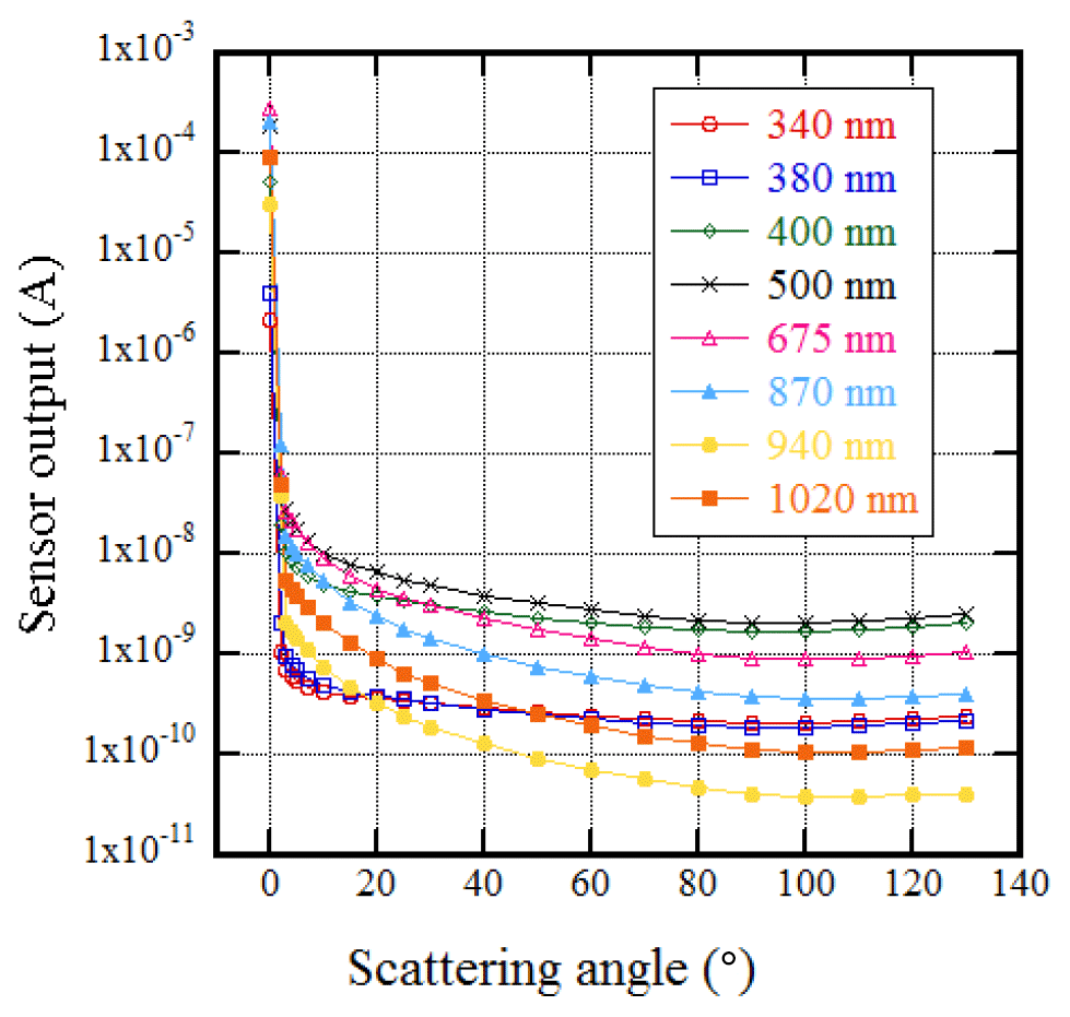
Figure 1 An example of sensor output for the solar direct irradiances and the scattered sky radiances by POM-02.

Table 2 shows the measurement ranges before and after modification of POM-02. POM-02 measures input energy in seven ranges according to the magnitude of the input energy, and the measured value is digitized with 15 bits. After modification, the measurement ranges are slightly expanded, and the measurement limit depends on the magnitude of the dark current and the magnitude of the noise. The sensor output takes into account the magnification of the amplifier, and the same amplifier was used for both the solar and lunar measurements.

Table 2 Measurement range before (current) and after modification (new) of POM-02. I_n and I_n−1 are the upper and lower limits of the current (unit: A), respectively.

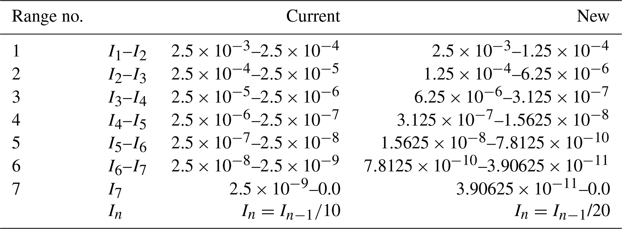
The dark current of the detector in the visible and near-infrared region was about $\mathrm{5}\times {\mathrm{10}}^{-\mathrm{13}}$ A, and the root mean square (rms) of the random component of the noise was $\mathrm{4}\times {\mathrm{10}}^{-\mathrm{14}}$ A. In consideration of these values, the new POM-02 can use amplifiers for measurement ranges 1 to 7 and the minimum meaningful current is about $\mathrm{4}\times {\mathrm{10}}^{-\mathrm{13}}$ A (∼ rms ×10) in the visible and near-infrared region. This value is smaller than the output for the direct solar irradiance by a factor of $\mathrm{1}\times {\mathrm{10}}^{-\mathrm{8}}$ to $\mathrm{1}\times {\mathrm{10}}^{-\mathrm{9}}$.

The dark current of the detector in the shortwave infrared wavelength region was about $\mathrm{1.5}\times {\mathrm{10}}^{-\mathrm{8}}$ A, and the rms of the random component of the noise was $\mathrm{4}\times {\mathrm{10}}^{-\mathrm{11}}$ A. The measurement range is limited due to the large dark current. The new POM-02 can use amplifiers for measurement ranges 1 to 5 and the minimum meaningful current is about $\mathrm{4}\times {\mathrm{10}}^{-\mathrm{10}}$ A (∼ rms ×10). This value and the magnitude of the measured value of the direct lunar irradiance are comparable. Therefore, it is difficult to measure the direct lunar irradiance even with the new POM-02 in the shortwave infrared wavelength region.

2.2 Sun and moon position sensor

The tracking of the Sun and the moon is based on the calculated position. The moon positions are calculated with the simplified formula in Nagasawa (1981). The necessary software is installed in the firmware of POM-02. Deviations may occur even if the instrument is pointed in the calculated direction due to errors in the moon position calculation, instrument installation errors, misalignment of the rotation axis, and so on. A position sensor is used to correct this deviation.

A position sensor with a four-quadrant detector is used to adjust the tracking of the Sun and the moon. In order to adjust the tracking of the moon, a position sensor incorporating a new electronic circuit to amplify the signal and new software to process the signal data were developed. The new position sensor can be used to track both the Sun and the moon.

When the input energy to the position sensor is small, it is difficult to adjust the tracking with the position sensor. The magnitude of the input energy to the position sensor varies depending on the lunar phase and the aerosol optical depth. It was confirmed that the function of the moon tracking adjustment works during the period of the full moon ± about 90^∘ of the phase angle (half-moon).

Whether the position sensor can be used can be determined by a user-specified threshold value. That is, the position sensor can be deactivated when the input energy to the position sensor becomes less than the threshold value. For phase angles larger than the half-moon, the signal of the position sensor was small, and the position sensor was deactivated.

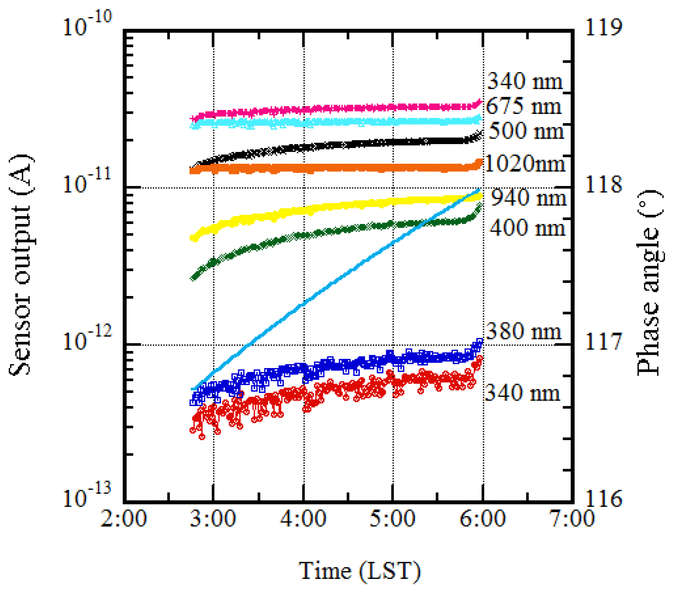
Figure 2 An example of the measurements taken on 14 October 2017 at NOAA/MLO. The phase angle of the moon (right y axis) is from 117.6 to 118.0^∘.

When the position sensor is not functioning, tracking is performed based on the calculated values. When comparing the moon position calculated by this simplified formula with that calculated using the NASA SPICE toolkit (Acton, 1996), the difference in the zenith angle is less than 0.01^∘, and the difference in the azimuth angle is less than 0.04^∘. The center of the field of view has a flat region of ±0.5^∘; the flat region is ±0.25^∘ in the solar disk scan. The apparent diameters of the Sun and the moon are about 0.5^∘. Since the calculation error of the moon position is less than 0.25^∘, if the misalignment of the rotation axis is negligible and POM-02 is installed correctly, it is possible to track the moon using only the calculated positions. In fact, measurements could be made on the day of a full moon ±10 d (phase angle about 120^∘). Figure 2 shows an example of the measurements on 14 October 2017 at NOAA/MLO. In this example, the phase angle of the moon is 117.6 to 118.0^∘.

3 ROLO irradiance model

In order to estimate the aerosol optical thickness using the moon as a light source, measurement of the extraterrestrial irradiance of the moon is necessary. In this study, a model known as the ROLO irradiance model (Kieffer and Stone, 2005) was used. This model was developed at USGS and is based on an extensive database of radiance images acquired by the ground-based ROLO over more than 8 years. ROLO is a NASA-funded program designed to use the moon for on-orbit calibration of Earth Observing System (EOS) satellite instruments. The empirical irradiance model was developed for 32 wavelengths from 350 to 2450 nm and has the same form for each wavelength. The average residual is less than 1 %. The coefficients of the empirical formula were constrained and determined using data with a phase angle between 1.55 and 97^∘. The empirically derived analytic form based on the primary geometric variables is as follows:

$$\begin{array}{}\text{(1)}& \begin{array}{rl}\ln A_k& =\sum _{i=\mathrm{0}}^{\mathrm{3}}{a}_{ik}{g}^i+\sum _{j=\mathrm{1}}^{\mathrm{3}}{b}_{jk}{\mathrm{\Phi }}^{\mathrm{2}j-\mathrm{1}}+c_{\mathrm{1}}\mathit{\varphi }+c_{\mathrm{2}}\mathit{\theta }+c_{\mathrm{3}}\mathrm{\Phi }\mathit{\varphi }\\ & +c_{\mathrm{4}}\mathrm{\Phi }\mathit{\theta }+d_{\mathrm{1}k}{e}^{-g/p_{\mathrm{1}}}+d_{\mathrm{2}k}{e}^{-g/p_{\mathrm{2}}}\\ & +d_{\mathrm{3}k}\cos \left(\right(g-p_{\mathrm{3}})/p_{\mathrm{4}}),\end{array}\end{array}$$

where A_k is the disk-equivalent reflectance, g is the absolute phase angle in radians, θ and ϕ are the selenographic latitude and longitude of the observer in degrees, and Φ is the selenographic longitude of the Sun in radians.

This formula must be used with caution. The equation in Kieffer and Stone (2005) has well-known typographical errors. In Eq. (1), θ and ϕ in the original expression by Kieffer and Stone (2005) are exchanged. In addition, the units of the coefficients p₁, p₂, p₃, and p₄ are degrees. Therefore, in order to make the dimensions the same, g in the exponent and the cosine terms must be converted into units of degrees.

The astronomical parameter was calculated using our own software developed using the NASA SPICE toolkit; an observation geometry information system named SPICE is offered by NASA's Navigation and Ancillary Information Facility (NAIF) (Acton, 1996). SPICE is widely used in the NASA and international planetary exploration communities (for more information about SPICE, refer to the NAIF webpage at http://naif.jpl.nasa.gov, last access: 2 December 2019).

In this study, only the values of the reflectance are used, and it is assumed that there is an error in the ROLO reflectance and that the correct reflectance is proportional to the ROLO reflectance. This indicates that the relative variation in the ROLO reflectance is assumed to be correct. The reflectance values are not converted to irradiance values by assuming the extraterrestrial solar spectral irradiance. The wavelength of POM-02 used in this study does not necessarily match the wavelength of the ROLO model. Here, the reflectance at the wavelength of POM-02 was calculated by linearly interpolating from the reflectance of the ROLO model at two adjacent wavelengths. Information on the filters used in the ROLO measurement was not available. Here, the wavelength is represented by the center wavelength. In addition, the ROLO model does not have reflectance data for the 340 nm wavelength. The reflectance at the 340 nm wavelength was obtained by extrapolating linearly from the values at the two end wavelengths.

4 Data

4.1 Data for Langley calibration

The aerosol optical thickness is estimated by measuring the attenuation of the direct solar or lunar irradiance. Therefore, in order to estimate the aerosol optical thickness, the output of the instrument for the input irradiance at the top of the atmosphere is necessary. The determination of this constant is referred to as calibration, and the output of the instrument for the extraterrestrial solar or lunar irradiance at the mean Earth–Sun distance (1 AU) at the reference temperature is called the calibration constant. In this study, the calibration constant was determined by the Langley method.

To calibrate the POM-02 by the Langley method, measurements were conducted at NOAA/MLO during the period from 28 September 2017 to 7 November 2017; the full moon was on 4 October and 3 November 2017. The MLO (19.5362^∘ N, 155.5763^∘ W) is located at an elevation of 3397.0 m a.m.s.l. on the northern slope of Mauna Loa, island of Hawaii, Hawaii, USA. The atmospheric pressure is about 680 hPa. The MLO is one of the most suitable places to obtain data for a Langley plot for the solar direct irradiance measurement (Shaw, 1983). Though the air at MLO is highly transparent, it is affected in the late morning and afternoon hours by marine aerosol that reaches the observatory during the marine inversion boundary layer breakdown under solar heating (Shaw, 1983; Perry et al., 1999). Therefore, using data taken in the morning is recommended (Shaw, 1982; Dutton et al., 1994; Holben et al., 1998).

However, during the nighttime, the upslope winds change to downslope winds, which bring low moisture and aerosol-poor air above the marine boundary layer down to the observatory. As a result, daytime orographic clouds at the observatory disappear and the atmosphere stratification becomes stable. These atmospheric conditions are suitable for obtaining data for the Langley plot from the lunar direct irradiance measurement.

During the calibration period, the data obtained for the moon over 18 nights for the visible and near-infrared region, and 13 nights for the short wavelength infrared region and water vapor channel (940 nm) were used to determine the calibration constants. The data obtained for the Sun over 22 d for the visible, near-infrared, and short wavelength infrared regions, and 24 d for the water vapor channel (940 nm) were used to determine the calibration constants.

4.2 Continuous measurement for comparison

The measurements for the estimation of the aerosol optical depth and precipitable water vapor were performed at 1 min intervals at the Japan Meteorological Agency/Meteorological Research Institute (JMA/MRI) (36.05^∘ N, 140.13^∘ E) in Tsukuba, which is located about 50 km northeast of Tokyo. The comparison was made using data obtained during the period from 1 January to 31 May 2018. During this period, the AOD and the precipitable water vapor (PWV) were estimated assuming the calibration constant was unchanged.

The optical depth estimated from POM-02 was compared with the value of the National Institute for Environmental Studies (NIES) High Spectral Resolution Lidar (HSRL; wavelength: 532 nm). The NIES/HSRL is one of the lidars operated by the lidar measurement group of the NIES (Shimizu et al., 2016). The NIES and MRI observation sites are located about 800 m apart. Since POM-02 was not measured at the 532 nm wavelength, the AOD at 532 nm was interpolated from the values of 500 and 675 nm by assuming that AOD is proportional to λ^−α, where λ is the wavelength. Furthermore, since the AOD of NIES/HSRL is the 15 min average, the value of POM-02 was also averaged over 15 min.

The PWV estimated from POM-02 was compared with that obtained from the vertical profile of a radiosonde and that obtained from the Global Positioning System (GPS) receiver. The radiosonde observation is operated from the JMA Aerological Observatory, which is adjacent to JMA/MRI. The GPS receiver is installed at JMA/MRI, and GPS data were processed by one of the JMA/MRI researchers (Shoji et al., 2013). The comparison of the PWV was performed using the 30 min average values.

5 Calibration of POM-02 using MLO data

5.1 Langley method

In this study, the calibration constant was determined by the Langley method (Uchiyama et al., 2018). Here, we do not consider the temperature dependence of the sensor output for the POM-02. Under these observation conditions in Tsukuba, the temperature dependence of the sensor output can be ignored except for the 340, 380, and 2200 nm channels (Uchiyama et al., 2018).

The sensor output when measuring the direct solar irradiance can be written as follows:

$$\begin{array}{}\text{(2)}& V\left({\mathit{\lambda }}_{\mathrm{0}}\right)={\displaystyle \frac{V_{S\mathrm{0}}\left({\mathit{\lambda }}_{\mathrm{0}}\right)}{R_S^{\mathrm{2}}}}\exp (-m(\mathit{\theta }\left)\mathit{\tau }\right({\mathit{\lambda }}_{\mathrm{0}}\left)\right){\stackrel{\mathrm{‾}}{T}}_{\mathrm{gas}}({\mathit{\lambda }}_{\mathrm{0}},\mathit{\theta }),\end{array}$$

where V(λ₀) is the sensor output in the λ₀ wavelength channel, R_S is the Earth–Sun distance in AU, m(θ) is the total air mass, τ(λ) is the total optical depth, θ is the solar zenith angle, and ${\stackrel{\mathrm{‾}}{T}}_{\mathrm{gas}}({\mathit{\lambda }}_{\mathrm{0}},\mathit{\theta })$ is the channel average transmittance of the gas line absorption. Furthermore, V_S0(λ₀) is the sensor output for the extraterrestrial solar irradiance at 1 AU and is called the calibration constant. τ(λ) consists of the optical thickness for molecular scattering (Rayleigh scattering), aerosol, and the continuous absorption of gas. In this study, it is assumed that air mass m(θ) is the same for all components. The air mass m(θ) for molecular scattering is used (Schmid and Wehrli, 1995; Holben et al., 1998).

In the case of no “gas absorption”, the following equation is used:

$$\begin{array}{}\text{(3)}& V\left({\mathit{\lambda }}_{\mathrm{0}}\right)={\displaystyle \frac{V_{S\mathrm{0}}\left({\mathit{\lambda }}_{\mathrm{0}}\right)}{R_S^{\mathrm{2}}}}\exp (-m(\mathit{\theta }\left)\mathit{\tau }\right({\mathit{\lambda }}_{\mathrm{0}}\left)\right).\end{array}$$

Taking the logarithm of the equation leads to

$$\begin{array}{}\text{(4)}& \begin{array}{rl}\ln \left(V\left({\mathit{\lambda }}_{\mathrm{0}}\right)R_S^{\mathrm{2}}\right)& =\ln V_{S\mathrm{0}}\left({\mathit{\lambda }}_{\mathrm{0}}\right)-m\left(\mathit{\theta }\right)\mathit{\tau }\left({\mathit{\lambda }}_{\mathrm{0}}\right)\\ & =C_{\mathrm{1}}m\left(\mathit{\theta }\right)+C_{\mathrm{2}}.\end{array}\end{array}$$

The parameters on the left-hand side are known: V is the measurement value, and R_S and m(θ) can be calculated from the solar zenith angle. For example, R_S can be calculated with the simplified formula in Nagasawa (1981), and m(θ) can be calculated as in Kasten and Young (1989). In the case of POM-02, the sensor output is the current, and the unit of the measurements of V is the ampere (A). C₂=ln V_S0 is determined from the ordinate intercept of a least-squares fit when one plots the left-hand side of the above equation versus air mass m(θ).

For the water vapor absorption band at a wavelength of 940 nm, the Beer–Lambert–Bouguer law is not valid. Calibration methods for the 940 nm channel, which is in the water vapor absorption band, have been considered extensively in previous studies (Reagan et al., 1987a, b, 1995; Bruegge et al., 1992; Thome et al., 1992, 1994; Michalsky et al., 1995, 2001; Schmid et al., 1996, 2001; Shiobara et al., 1996; Halthore et al., 1997; Cachorro et al., 1998; Plana-Fattori et al., 1998, 2004; Ingold et al., 2000; Kiedron et al., 2001, 2003; Uchiyama et al., 2014, Campanelli et al., 2014).

In this study, the modified Langley method is used (Reagan et al., 1987a; Bruegge et al., 1992; Schmid and Wehrli, 1995). In the modified Langley method, the transmittance is approximated by an empirical formula. The water vapor transmittance is approximated as follows:

$$\begin{array}{}\text{(5)}& Tr\left({\mathrm{H}}_{\mathrm{2}}\mathrm{O}\right)=\exp (-a(m\left(\mathit{\theta }\right)\cdot \mathrm{pwv}{)}^b),\end{array}$$

where a and b are fitting coefficients, and pwv is PWV.

Coefficients a and b were determined by computing the transmittance for several atmospheric models (Uchiyama et al., 2014).

The output of the 940 nm channel can be written as follows:

$$\begin{array}{}\text{(6)}& \begin{array}{rl}V\left({\mathit{\lambda }}_{\mathrm{0}}\right)& ={\displaystyle \frac{V_{S\mathrm{0}}\left({\mathit{\lambda }}_{\mathrm{0}}\right)}{R_S^{\mathrm{2}}}}\exp (-m(\mathit{\theta }\left)\mathit{\tau }\right({\mathit{\lambda }}_{\mathrm{0}}\left)\right)Tr\left({\mathrm{H}}_{\mathrm{2}}\mathrm{O}\right)\\ & ={\displaystyle \frac{V_{S\mathrm{0}}\left({\mathit{\lambda }}_{\mathrm{0}}\right)}{R_S^{\mathrm{2}}}}\exp (-m(\mathit{\theta }\left)\mathit{\tau }\right({\mathit{\lambda }}_{\mathrm{0}}\left)\right)\\ & \exp (-a(m\left(\mathit{\theta }\right)\cdot \mathrm{pwv}{)}^b).\end{array}\end{array}$$

Taking the logarithm of the equation leads to

$$\begin{array}{}\text{(7)}& \begin{array}{rl}\ln V{R}_s^{\mathrm{2}}+m\left(\mathit{\theta }\right)({\mathit{\tau }}_{\mathrm{aer}}+{\mathit{\tau }}_R)& =\ln V_{S\mathrm{0}}-a\left(\mathrm{pwv}{)}^{b}m\right(\mathit{\theta }{)}^b\\ & =C_{\mathrm{1}}^{\prime }m(\mathit{\theta }{)}^b+C_{\mathrm{2}}^{\prime }.\end{array}\end{array}$$

In the same way as the normal Langley method, the parameters on the left-hand side are known: V is the measurement value, and R_S and m(θ) can be calculated from the solar zenith angle. τ_R is also estimated from the surface pressure; for example, τ_R can be calculated as in Asano et al. (1983). In addition, τ_aer is the aerosol optical depth at the 940 nm wavelength, which is interpolated from the aerosol optical depth from the values at the 870 and 1020 nm wavelengths.

If pwv is constant, then the right-hand side of the equation is a linear function of m(θ)^b. Therefore, the values on the left-hand side can be fitted by a linear function of m(θ)^b, and the intersection of the y axis and the fitted line is ln V_S0.

5.2 Langley method for the moon

The sensor output when measuring the direct lunar irradiance can be written as follows:

$$\begin{array}{}\text{(8)}& \begin{array}{rl}V\left({\mathit{\lambda }}_{\mathrm{0}}\right)& ={\displaystyle \frac{{\stackrel{\mathrm{̃}}{A}}_{\mathrm{ROLO}}}{\mathit{\pi }}}{\mathrm{\Omega }}_{\mathrm{M}}{\displaystyle \frac{V_{S\mathrm{0}}\left({\mathit{\lambda }}_{\mathrm{0}}\right)}{R_S^{\mathrm{2}}}}\cdot {\displaystyle \frac{\mathrm{1}}{R_{\mathrm{m}}^{\mathrm{2}}}}\\ & \exp (-m(\mathit{\theta }\left)\mathit{\tau }\right({\mathit{\lambda }}_{\mathrm{0}}\left)\right){\stackrel{\mathrm{‾}}{T}}_{\mathrm{gas}}({\mathit{\lambda }}_{\mathrm{0}},\mathit{\theta }),\end{array}\end{array}$$

where Ω_M is the solid angle of the moon, R_S is the distance between the moon and the Sun in AU, and R_m is the distance between the moon and the observer normalized by 384 400 km (the mean radius of the moon's orbit around the Earth). ${\stackrel{\mathrm{̃}}{A}}_{\mathrm{ROLO}}$ is the smoothed ROLO reflectance adjusted to the laboratory reflectance spectra of the Apollo 16 samples. ${\stackrel{\mathrm{̃}}{A}}_{\mathrm{ROLO}}$ is calculated using the lunar reflectance A_ROLO with the ROLO irradiance model by the method shown in Kieffer and Stone (2005) (see Appendix A).

Let ${\stackrel{\mathrm{̃}}{A}}_{\mathrm{ROLO}}=F_C{A}_{\mathrm{ROLO}}$, where F_C is a constant for smoothing (see Appendix A). Using this equation, Eq. (8) becomes

$$\begin{array}{}\text{(9)}& \begin{array}{rl}V\left({\mathit{\lambda }}_{\mathrm{0}}\right)& ={\displaystyle \frac{F_C{A}_{\mathrm{ROLO}}}{\mathit{\pi }}}{\mathrm{\Omega }}_{\mathrm{M}}{\displaystyle \frac{V_{S\mathrm{0}}\left({\mathit{\lambda }}_{\mathrm{0}}\right)}{R_S^{\mathrm{2}}}}\cdot {\displaystyle \frac{\mathrm{1}}{R_{\mathrm{m}}^{\mathrm{2}}}}\\ & \exp (-m(\mathit{\theta }\left)\mathit{\tau }\right({\mathit{\lambda }}_{\mathrm{0}}\left)\right){\stackrel{\mathrm{‾}}{T}}_{\mathrm{gas}}({\mathit{\lambda }}_{\mathrm{0}},\mathit{\theta }).\end{array}\end{array}$$

It is known that the aerosol optical depth retrieved using the ROLO reflectance contains an error, which is dependent on the phase angle (Barreto et al., 2016, 2017, 2019; Juryšek and Prouza, 2017). We assume that there is an error in the ROLO reflectance and that the correct lunar reflectance is proportional to the ROLO reflectance. This indicates that the relative variation in the ROLO model reflectance is assumed to be correct. Let the proportional constant be denoted C^′, and A_ROLO in Eq. (9) be replaced with $C^{\prime }\cdot A_{\mathrm{ROLO}}$. Equation (9) then becomes

$$\begin{array}{}\text{(10)}& \begin{array}{rl}V\left({\mathit{\lambda }}_{\mathrm{0}}\right)& ={\displaystyle \frac{F_C{C}^{\prime }{A}_{\mathrm{ROLO}}}{\mathit{\pi }}}{\mathrm{\Omega }}_{\mathrm{M}}{\displaystyle \frac{V_{S\mathrm{0}}\left({\mathit{\lambda }}_{\mathrm{0}}\right)}{R_S^{\mathrm{2}}}}\cdot {\displaystyle \frac{\mathrm{1}}{R_{\mathrm{m}}^{\mathrm{2}}}}\\ & \exp (-m(\mathit{\theta }\left)\mathit{\tau }\right({\mathit{\lambda }}_{\mathrm{0}}\left)\right){\stackrel{\mathrm{‾}}{T}}_{\mathrm{gas}}({\mathit{\lambda }}_{\mathrm{0}},\mathit{\theta })\\ & ={\displaystyle \frac{C{A}_{\mathrm{ROLO}}}{\mathit{\pi }}}{\mathrm{\Omega }}_{\mathrm{M}}{\displaystyle \frac{V_{S\mathrm{0}}\left({\mathit{\lambda }}_{\mathrm{0}}\right)}{R_S^{\mathrm{2}}}}\cdot {\displaystyle \frac{\mathrm{1}}{R_{\mathrm{m}}^{\mathrm{2}}}}\\ & \exp (-m(\mathit{\theta }\left)\mathit{\tau }\right({\mathit{\lambda }}_{\mathrm{0}}\left)\right){\stackrel{\mathrm{‾}}{T}}_{\mathrm{gas}}({\mathit{\lambda }}_{\mathrm{0}},\mathit{\theta }),\end{array}\end{array}$$

where F_CC^′ is substituted with C.

In the case of no “gas absorption”, taking the logarithm of the equation leads to

$$\begin{array}{}\text{(11)}& \begin{array}{rl}\ln \left({\displaystyle \frac{\mathit{\pi }V\left({\mathit{\lambda }}_{\mathrm{0}}\right)}{A_{\mathrm{ROLO}}{\mathrm{\Omega }}_{\mathrm{M}}}}{R}_S^{\mathrm{2}}{R}_{\mathrm{m}}^{\mathrm{2}}\right)& =\ln C{V}_{S\mathrm{0}}\left({\mathit{\lambda }}_{\mathrm{0}}\right)-m\left(\mathit{\theta }\right)\mathit{\tau }\left({\mathit{\lambda }}_{\mathrm{0}}\right)\\ & =\ln V_{m\mathrm{0}}\left({\mathit{\lambda }}_{\mathrm{0}}\right)-m\left(\mathit{\theta }\right)\mathit{\tau }\left({\mathit{\lambda }}_{\mathrm{0}}\right)\\ & =C_{\mathrm{1}}^{\prime \prime }m\left(\mathit{\theta }\right)+C_{\mathrm{2}}^{\prime \prime },\end{array}\end{array}$$

where V_m0(λ₀)=CV_S0(λ₀). $C_{\mathrm{2}}^{\prime \prime }=\ln V_{m\mathrm{0}}$ is determined from the ordinate intercept of a least-squares fit when one plots the left-hand side of the above equation versus air mass m(θ).

V_S0 can be determined by applying the Langley method to data taken during the daytime. If V_S0 is determined, the coefficient C can be determined by taking the ratio of V_m0 and V_S0. If the coefficient C is 1, the reflectance of the ROLO model will be correct. If the coefficient C is greater than 1 (less than 1), the reflectance in the ROLO model is underestimated (overestimated).

5.3 Results

Examples of Langley plots in the visible and near-infrared wavelengths are shown in Fig. 3. In these examples, the regression lines can be well determined for any wavelength. $C_{\mathrm{2}}^{\prime \prime }=\ln V_{m\mathrm{0}}$ is determined from the ordinate intercept of the regression line (see Eq. 11). At the 340 nm wavelength, the regression line tends to deviate from the measured values in the region of air masses larger than 6. It is presumed that the detector output at the 340 nm wavelength is small and hence may be nonlinear. The output at the time of observation was about $\mathrm{1}\times {\mathrm{10}}^{-\mathrm{12}}$ A. When using output values less than this, the user needs to treat their results with caution. At the 940 nm wavelength, the modified Langley method was applied. In this example, the regression line provides a good fit.

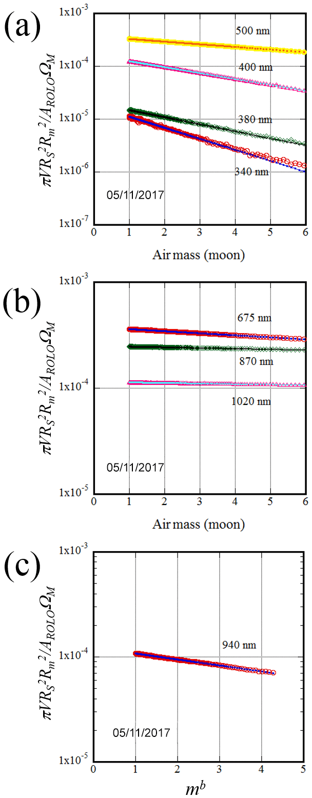
Figure 3 Examples of the Langley plot in the visible and near-infrared region on 5 November 2017. The y axis is the equation in parentheses on the left-hand side of Eq. (11). (a) 340, 380, 400, 500 nm; (b) 675, 870, 1020 nm; (c) 940 nm, modified Langley method.

Figure 4 Examples of the Langley plot in the shortwave infrared region.

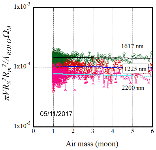
In Fig. 4, examples of the Langley plot in the shortwave infrared region (1225, 1627, and 2200 nm) are shown. The detector output of these channels ranges from $\mathrm{2}\times {\mathrm{10}}^{-\mathrm{10}}$ to $\mathrm{5}\times {\mathrm{10}}^{-\mathrm{10}}$ A, and the root mean square error of the random noise is $\mathrm{4}\times {\mathrm{10}}^{-\mathrm{11}}$ A. The ratio of noise to detector output is large, and it is difficult to use these channels for estimating the aerosol optical depth.

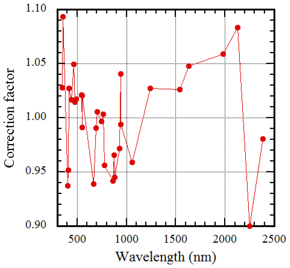
Figure 5 Relationship between phase angle and reflectance correction factor $C=V_{m\mathrm{0}}/V_{S\mathrm{0}}$ in the visible and near-infrared region. A regression curve ($C=A_c\cdot g^{\mathrm{2}}+B_c$, g: phase angle) was also plotted.

In Fig. 5, the relationship between the coefficient $C(=V_{m\mathrm{0}}/V_{S\mathrm{0}})$ and the phase angle in the visible and near-infrared wavelength region (from 340 to 1020 nm) is shown. As shown in the previous section, the corrected lunar reflectance is assumed to be proportional to the ROLO reflectance, and the proportional coefficient C is the ratio of the calibration constant for the moon and the Sun. That is, the coefficient C indicates the error of the ROLO reflectance, and thus more accurate reflectance can be obtained by multiplying the ROLO reflectance by the coefficient C. As can be seen from this figure, the coefficient C is often greater than 1 and depends on the phase angle. At most wavelengths, the coefficient C is small when the absolute value of the phase angle is small (near the full moon) and increases as the absolute value of the phase angle increases. The range of C is 0.95 to 1.18. The absorption band of water vapor is at the 940 nm wavelength. Water vapor in the atmosphere tends to fluctuate. Therefore, it is difficult to make accurate Langley plots, and the accuracy of both V_S0 and V_m0 is poor. Therefore, no clear relationship between C and the phase angle is found, but the coefficient C is about 1.16. The fact that C is larger than 1 means that the reflectance of the ROLO irradiance model is underestimated.

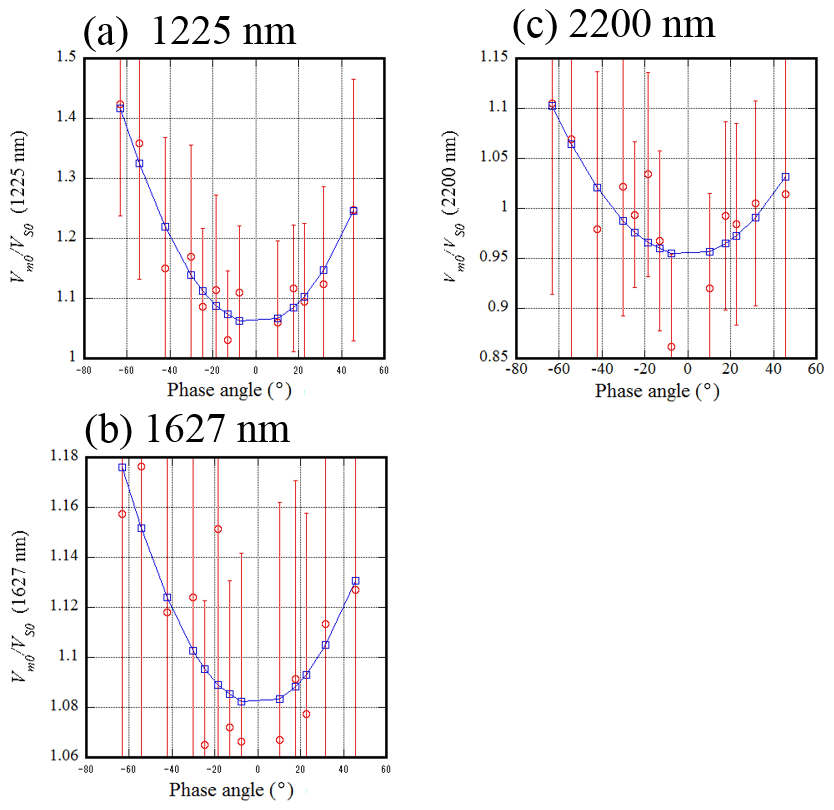
Figure 6 Relationship between phase angle and reflectance correction factor $C=V_{m\mathrm{0}}/V_{S\mathrm{0}}$ in the shortwave infrared region. A regression curve ($C=A_c\cdot g^{\mathrm{2}}+B_c$, g: phase angle) was also plotted.

In Fig. 6, the relationship between the coefficient $C(=V_{m\mathrm{0}}/V_{S\mathrm{0}})$ and the phase angle in the shortwave infrared wavelength region (1225, 1627, and 2200 nm) is shown. In these channels, the error for C is large, but the coefficient C depends on the phase angle as in the visible and near-infrared wavelength region; C is small when the phase angle is near zero and increases as the absolute value of the phase angle increases.

In this study, the phase angle dependence of the coefficient C is approximated by a quadratic equation of the absolute value of the phase angle:

$$\begin{array}{}\text{(12)}& C=A_c\cdot g^{\mathrm{2}}+B_c,\end{array}$$

where g is the phase angle.

That is,

$$\begin{array}{}\text{(13)}& V_{m\mathrm{0}}=V_{S\mathrm{0}}\cdot (A_c\cdot g^{\mathrm{2}}+B_c).\end{array}$$

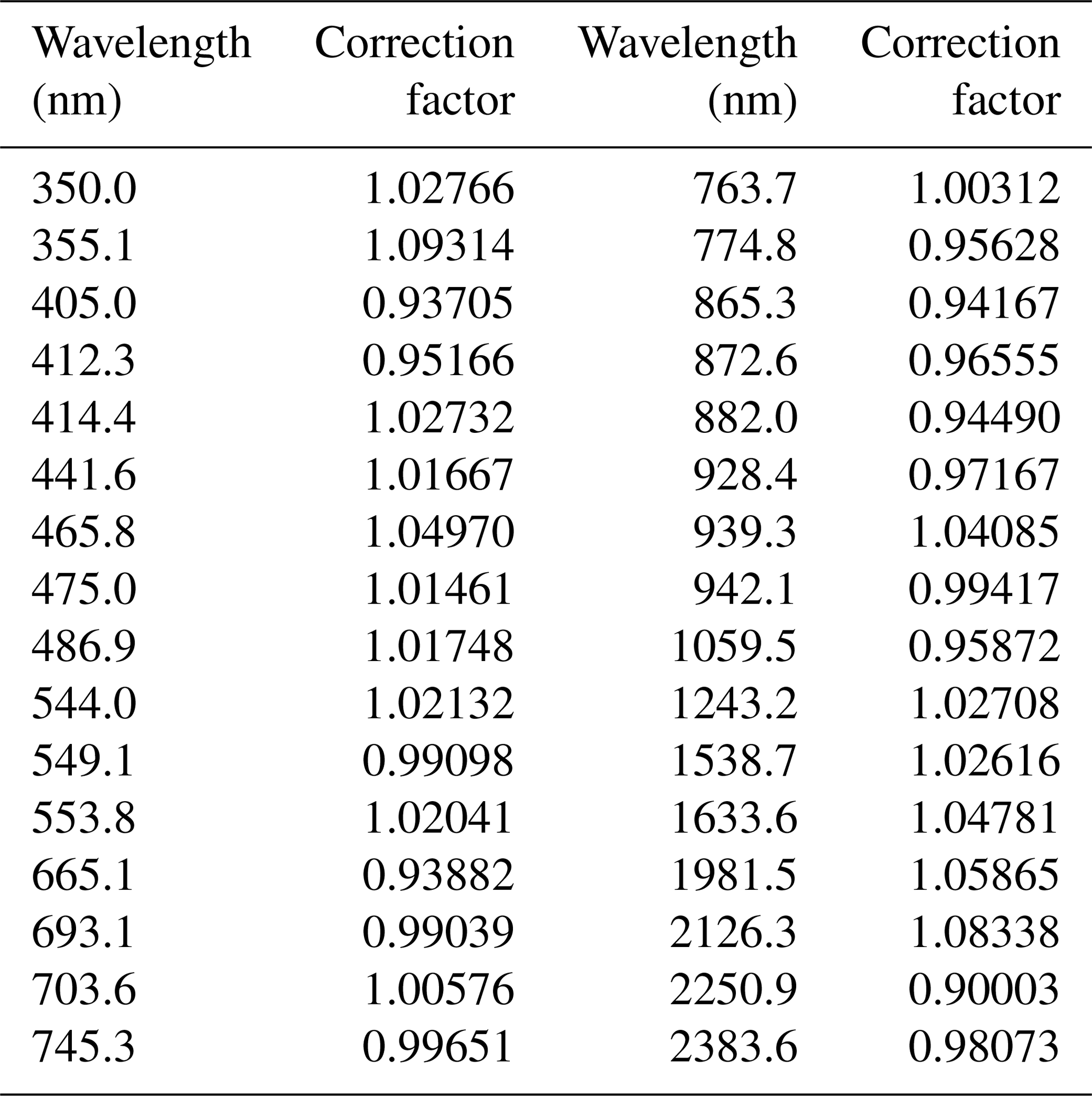
The coefficients A_c and B_c are shown in Table 3. The regression line was plotted in Figs. 5 and 6. By using this approximation, the reflectance of the ROLO model can be estimated to within 1 % in most channels. By using this approximation, the data processing to estimate the aerosol optical depth from the measured value becomes straightforward. The coefficients, F_C, for smoothing the ROLO reflectance are also shown in Table 3. The coefficients $A_c^{\prime }$ and $B_c^{\prime }$ of the regression equation when using the smoothed ROLO reflectance are also given.

Table 3 Coefficients of the regression equation for reflectance correction factor C.

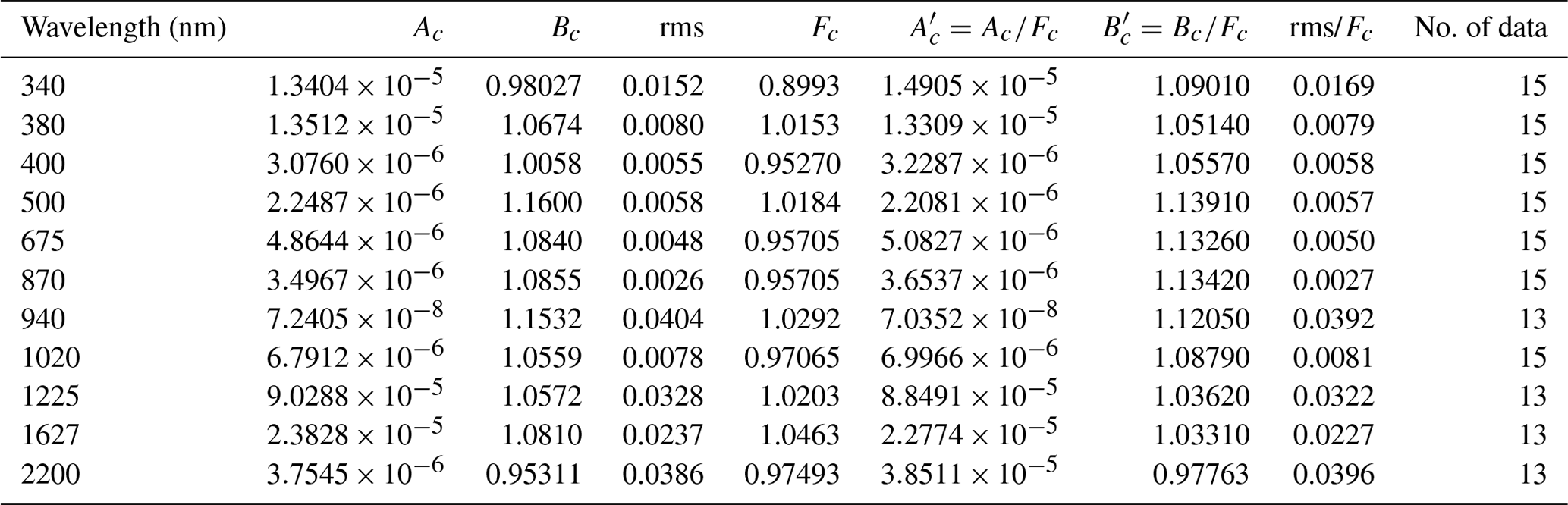
$C=A_c\cdot g^{\mathrm{2}}+B_c$. g: phase angle (degrees). F_c: smoothing factor

The size of the error in the reflectance in the ROLO irradiance model is dependent on the phase angle. The ROLO reflectance was obtained by dividing the lunar irradiance measured by Kieffer and Stone (2005) by the solar spectral irradiance of the 1985 Wehrli Standard Extraterrestrial Solar Irradiance Spectrum (Wehrli, 1985: Neckel and Labs, 1981). The solar spectral irradiances are dependent on the solar spectral models. Therefore, the ROLO reflectance includes an error due to the error in the solar spectral irradiance of 1985 Wehrli. Instrument performance, data processing, and so on are also sources of error. In this study, C is approximated as a symmetric quadratic equation of the phase angle, but the phase angle dependence of C is asymmetric (see Figs. 5 and 6). The applicable range of the ROLO reflectance model is a phase angle of about 95^∘ or less. In order to improve the accuracy of the ROLO reflectance model and expand its application range, it is necessary to further accumulate the reflectance data of the moon.

6 Results of comparison

In order to validate the estimations of AOD and PWV, we compared them with the AOD and PWV obtained by independent methods. We investigated whether there is a difference between daytime and nighttime measurements, and compared the measurements for the daytime and nighttime with measurement data which were recorded independently of POM-02 and have the same accuracy and precision in the daytime and nighttime.

Furthermore, the continuity of the AOD and PWV before and after sunrise and sunset was investigated, and the AOD and PWV of AERONET and POM-02 at MLO were also compared.

6.1 AOD

The AOD estimated from POM-02 was compared with the value of the NIES/HSRL (wavelength: 532 nm).

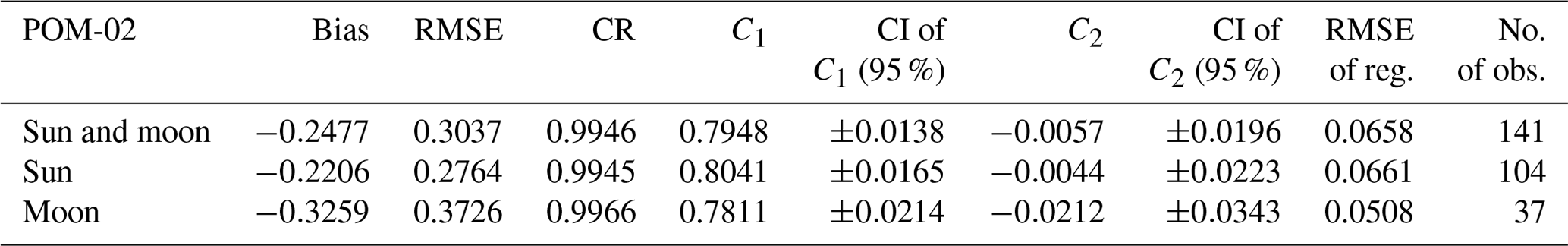
Figure 7a and b show the scatter plot of the aerosol optical depth during the daytime and nighttime, respectively. In Fig. 7c, the scatter plot during the nighttime is shown together with that during the daytime. Table 4 shows the results of the comparison between NIES/HSRL and POM-02 AOD: the statistics of the difference between the two AODs, the coefficients of the linear regression equation of NIES/HSRL and POM-02 AOD (${\mathit{\tau }}_{\mathrm{HSRL}}=C_{\mathrm{1}}\cdot {\mathit{\tau }}_{\mathrm{POM}\mathrm{02}}+C_{\mathrm{2}})$, the root mean square error (RMSE) of the residual, the 95 % confidence interval of the coefficients, and the number of observations.

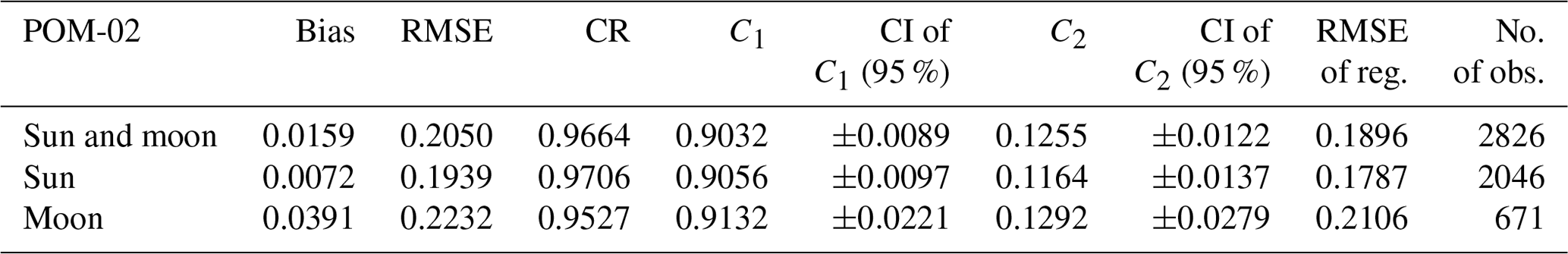
Table 4 Results of the comparison between NIES/HSRL and POM-02 aerosol optical depth.

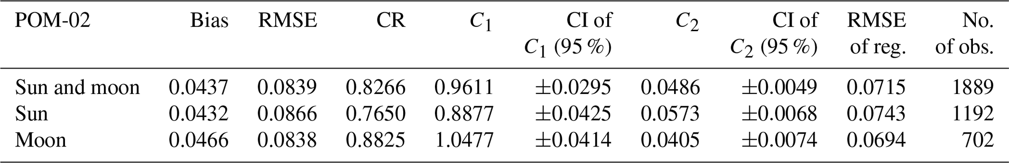
RMSE: root mean square error. CR: correlation coefficient. C₁ and C₂: coefficients of regression line (${\mathit{\tau }}_{\mathrm{HSRL}}=C_{\mathrm{1}}\cdot {\mathit{\tau }}_{POM-\mathrm{02}}+C_{\mathrm{2}}$). CI of C₁ (95 %): 95 % confidential interval of C₁. CI of C₂ (95 %): 95 % confidential interval of C₂. RMSE of reg.: RMSE of regression line.

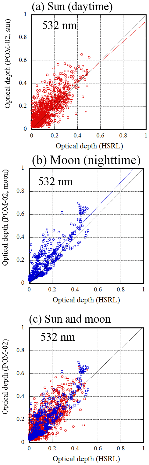
Figure 7 Scatter plot of HSRL and POM-02 aerosol optical depth at 532 nm: (a) daytime (red), (b) nighttime (blue), and (c) overlapping daytime (red) with nighttime (blue).

The difference in the slope value of the regression coefficients is 0.1600 ($=\mathrm{1.0477}-\mathrm{0.8877}$). The 95 % confidence interval of the coefficient is about ±0.04 during both the daytime and the nighttime. It cannot be said that the slopes of the two regression lines are equal based on their 95 % confidence intervals. However, the correlation between NIES/HSRL and POM-02 AOD is high, and the differences between them and their RMSEs are similar. Furthermore, as shown in Fig. 7c, the scatter diagrams for the daytime and nighttime are almost overlapping, and it seems that the two sets of measurements obtained similar results.

Examples of time series of the AOD from NIES/HSRL and POM-02 are shown in Fig. 8. As can be seen from these figures, the AODs of the daytime and nighttime estimated from POM-02 constitute a continuous series. The AOD from NIES/HSRL and that from POM-02 have qualitatively similar time variations. However, in these limited examples, while there are periods when the values are consistent, there are periods when there are systematic differences.

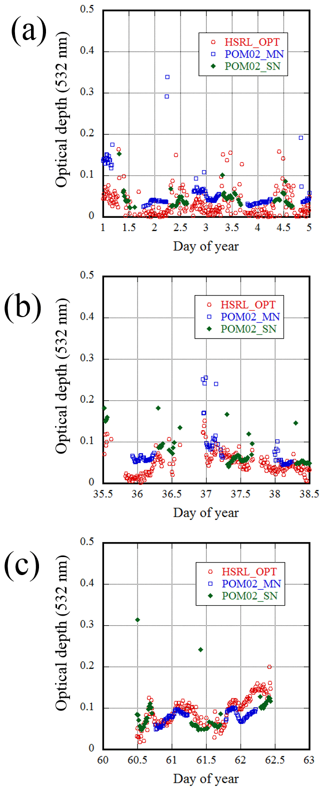
Figure 8 Examples of time series of HSRL (red), POM-02 daytime (green), and nighttime (blue) aerosol optical depths at 532 nm. The phase angles (g) during the measurement periods were (a) $g=-\mathrm{21.863}$ to 35.881^∘, (b) g=47.454 to 83.190^∘, and (c) $g=-\mathrm{19.150}$ to 21.573^∘.

In the NIES/HSRL data processing, the AOD below an altitude of 500 m is calculated by using the value of the extinction coefficient for an altitude of 500 m. Since the height of the atmospheric boundary layer is typically 1500 to 2000 m, a large amount of aerosols exist at altitudes below 500 m. If the actual distribution deviates from the assumed distribution, the estimated AOD is shifted systematically.

In Fig. 8, only limited examples were shown, but in the Supplement, the time series of the AOD at 500 nm at Tsukuba for 5 months is shown in Fig. S1. In addition, the time series of the comparison between the HSRL and POM-02 AOD for 5 months is shown in Fig. S3.

6.2 PWV

The PWV estimated from POM-02 was compared with that obtained from the vertical profile of the radiosonde and that obtained from the GPS receiver. The PWV estimated from the radiosonde data has a frequency of two values per day, whereas the PWV obtained from GPS is continuous.

6.2.1 Radiosonde

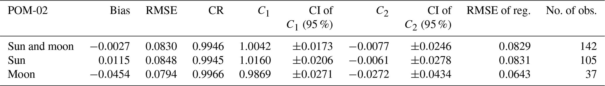
The PWV from a radiosonde is often used as a reference for the PWV measurement value. The PWV from the radiosonde and PWV from POM-02 are first compared. Figure 9 shows a scatter plot of the PWV from the radiosonde and from POM-02. The red symbol denotes 00:00 UTC (09:00 LST), and the blue symbol is 12:00 UTC (21:00 LST). Table 5 shows the results of the comparison between the radiosonde and POM-02 precipitable water vapor (Table 5 is the same as Table 4 except for radiosonde and POM-02 precipitable water vapor).

Table 5 Same as Table 4 except for radiosonde and POM-02 precipitable water vapor.

PWV, bias, RMSE, RMSE of reg.: g cm⁻². C₁ and C₂: coefficients of regression line (${\mathrm{PWV}}_{\mathrm{POM}-\mathrm{02}}=C_{\mathrm{1}}\cdot {\mathrm{PWV}}_{\mathrm{Sonde}}+C_{\mathrm{2}}$).

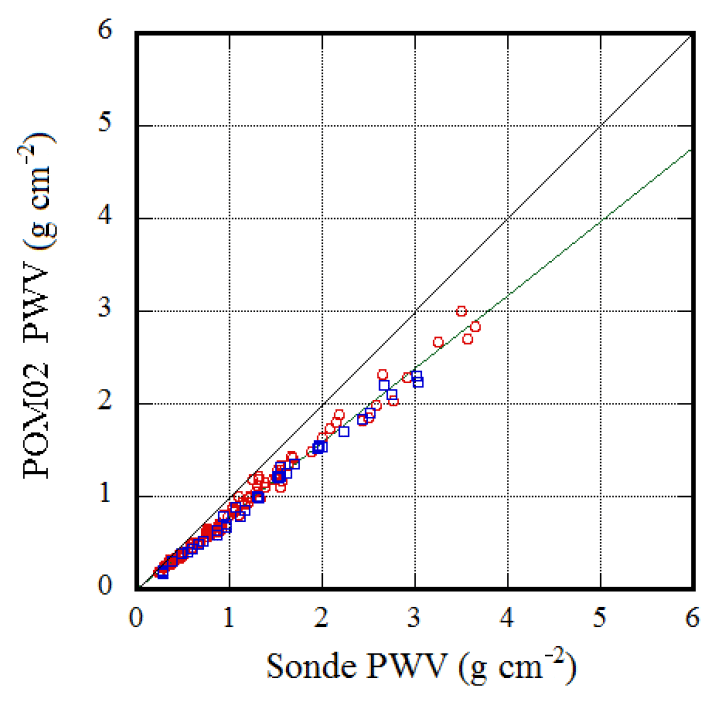
Figure 9 Scatter plot of radiosonde and POM-02 precipitable water vapor. Daytime (nighttime) measurements are indicated by a red (blue) symbol.

The ratio of PWV estimated from POM-02 and the radiosonde in both daytime and nighttime is almost constant: the slope of the regression line is 0.80 in the daytime and 0.78 in the nighttime.

The empirical formula of the transmittance is expressed as Eq. (5). The ratio of the two PWVs is almost constant. In addition, as shown in Fig. 5, the modified Langley plot provides a good fit for the data. From these facts, it seems that the value of the coefficient b in Eq. (5) is appropriate but the value of the coefficient a in Eq. (5) was inappropriate. It is possible that the filter characteristics of the 940 nm channel have changed from the nominal characteristics due to degradation.

Let $\mathrm{pwv}=c\cdot {\mathrm{pwv}}^{\prime }$ and rewrite Eq. (5) as follows:

$$\begin{array}{}\text{(14)}& \begin{array}{rl}Tr\left({\mathrm{H}}_{\mathrm{2}}\mathrm{O}\right)& =\exp (-a(m\left(\mathit{\theta }\right)\cdot (c\cdot {\mathrm{pwv}}^{\prime }){)}^b)\\ & =\exp (-a{c}^b(m\left(\mathit{\theta }\right)\cdot {\mathrm{pwv}}^{\prime }{)}^b).\end{array}\end{array}$$

Then, the PWV can be corrected by replacing a with ac^b.

Figure 10 shows a scatter plot of the PWV from the radiosonde and the corrected PWV from POM-02. For the correction coefficient c, the average value of the coefficients C₁ of the daytime and nighttime regression equations was used. Table 6 shows the results of the comparison between the radiosonde and corrected POM-02 precipitable water vapor (Table 6 is the same as Table 4 except for radiosonde and corrected POM-02 precipitable water vapor).

Table 6 Same as Table 4 except for radiosonde and corrected POM-02 precipitable water vapor.

C₁ and C₂: coefficients of regression line (${\mathrm{PWV}}_{\mathrm{POM}-\mathrm{02}}\left(\mathrm{corrected}\right)=C_{\mathrm{1}}\cdot {\mathrm{PWV}}_{\mathrm{Sonde}}+C_{\mathrm{2}}$).

Figure 10 Same as Fig. 9 except for corrected POM-02 precipitable water vapor.

The slope C₁ of the regression line during the daytime and nighttime is 1.0160 and 0.9869, respectively, and the difference between them is 0.0291 ($=\mathrm{1.0160}-\mathrm{0.9869}$). The 95 % confidence intervals of the slopes during the daytime and nighttime are ±0.0206 and ±0.0271, respectively. The difference between them is 0.0291, which is larger than the respective 95 % confidence intervals. Therefore, the two slopes are not equivalent based on the 95 % confidence intervals.

However, since the slope of the regression line determined using all of the data is 1.0042 and the 95 % confidence interval is ±0.0173, the three slopes of the regression lines can be regarded as equivalent at the 95 % confidence level. Furthermore, there are no large differences in the bias, RMSE, and correlation coefficient between PWV from the radiosonde and POM-02. Therefore, the PWVs of daytime and nighttime for POM-02 are statistically equivalent. That is, both PWVs are presumed to have the same degree of precision and accuracy within the measurement uncertainty.

6.2.2 GPS

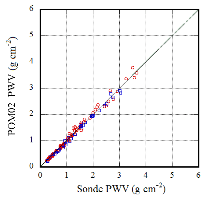
Next, the result of the comparison between the PWV obtained from POM-02 and GPS is shown. Before that, the result of the comparison between the PWV obtained from GPS and the radiosonde is shown in Fig. 11. Table 7 shows the results of the comparison between GPS and radiosonde precipitable water vapor (Table 7 is the same as Table 4 except for GPS and radiosonde precipitable water vapor).

Table 7 Same as Table 4 except for GPS and radiosonde precipitable water vapor.

C₁ and C₂: coefficients of regression line (${\mathrm{PWV}}_{\mathrm{Sonde}}=C_{\mathrm{1}}\cdot {\mathrm{PWV}}_{\mathrm{GPS}}+C_{\mathrm{2}}$).

Figure 11 Scatter plot of GPS and radiosonde precipitable water vapor.

The slope of the regression line in Fig. 11 is about 0.94. In the region of the PWV of less than 2 g cm⁻², the PWV from GPS tends to be smaller than the PWV from the radiosonde. In the region of PWV of more than 3 g cm⁻², the difference between PWV from GPS and the radiosonde is more scattered. Therefore, the slope of the regression line became smaller than 1. In a previous comparison conducted by the authors, the slope of the regression line was almost 1 (Uchiyama et al., 2014). There is a possibility that the PWV from GPS used in this study has a larger error than the PWV used previously.

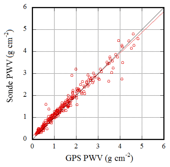
Figure 12 Scatter plot of PWV from GPS and corrected PWV from POM-02: (a) daytime (red), (b) nighttime (blue), and (c) overlapping daytime (red) with nighttime (blue).

Figure 12 shows a scatter diagram of the PWV from GPS and the corrected PWV from POM-02. Table 8 shows the results of the comparison between PWV from GPS and corrected PWV from POM-02 (Table 8 is the same as Table 4 except for GPS and corrected POM-02 precipitable water vapor).

Table 8 Same as Table 4 except for GPS and corrected POM-02 precipitable water vapor.

C₁ and C₂: coefficients of regression line (${\mathrm{PWV}}_{\mathrm{POM}-\mathrm{02}}\left(\mathrm{corrected}\right)=C_{\mathrm{1}}\cdot {\mathrm{PWV}}_{\mathrm{GPS}}+C_{\mathrm{2}}$).

The slope of the regression line is about 0.91 for both the daytime and nighttime. Similar to the results of the comparison between the PWV from the radiosonde and GPS, in the region of PWV from GPS less than 2 g cm⁻², the PWV from GPS tends to be somewhat smaller than the PWV from POM-02 during both the daytime and nighttime. In the region of PWV greater than 3 g cm⁻², the difference between the PWV from GPS and the radiosonde is more scattered.

The difference between the slopes of the regression lines is 0.0076 ($=\mathrm{0.9132}-\mathrm{0.9056}$) and the 95 % confidence intervals during the daytime and nighttime are ±0.0097 and ±0.0221, respectively. Therefore, the confidence intervals of the two slopes are overlapping, and the values of slopes can be regarded as equivalent at the 95 % confidence level.

In Fig. 12c, the scatter plot obtained using nighttime data is shown together with that obtained using daytime data. The data obtained during the daytime and nighttime overlap, and it seems that the PWV from POM-02 during the daytime and nighttime are estimated with the same degree of precision and accuracy.

Examples of time series of PWV from GPS and POM-02 are shown in Fig. 13. The PWV from GPS and that from POM-02 have qualitatively similar time variations. In these limited examples, although there are some systematic differences in Fig. 13b, the PWV from GPS and the PWV from POM-02 almost overlap in Figs. 13a and c. In addition, the PWV during the daytime and nighttime estimated from POM-02 are continuously connected.

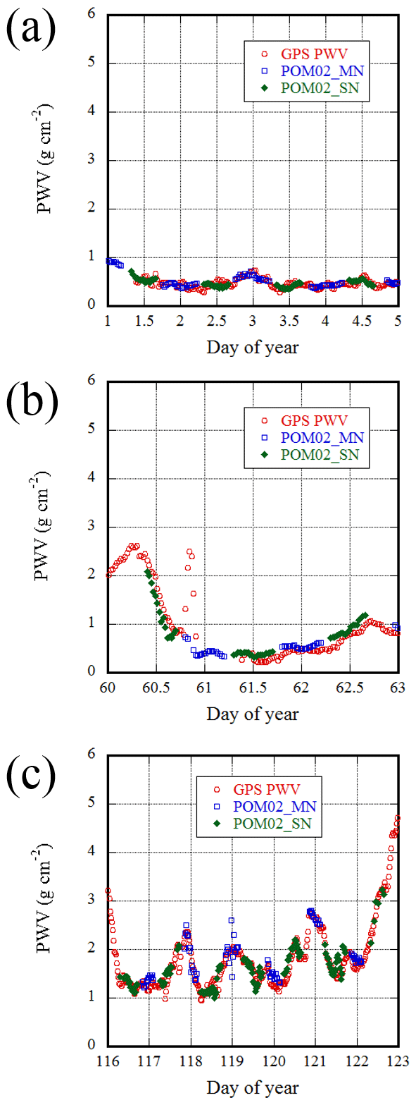
Figure 13 Examples of time series of GPS (red), POM-02 daytime (green), and nighttime (blue) corrected precipitable water vapor. The phase angles (g) during the measurement periods were (a) $g=-\mathrm{21.863}$ to 35.881^∘, (b) $g=-\mathrm{19.150}$ to 21.573^∘, and (c) $g=-\mathrm{55.145}$ to 30.611^∘.

In Fig. 13, only limited examples were shown, but in the Supplement, the time series of the PWV at Tsukuba for 5 months is shown in Fig. S2. In addition, the time series of the comparison between GPS and POM-02 PWV for 5 months is shown in Fig. S4.

6.3 Comparison of AOD (PWV) before and after sunrise and sunset

The comparison of the AOD (PWV) before and after sunrise and sunset is used to evaluate the moon photometry (Berkoff et al., 2011; Barreto et al., 2013, 2016, 2017, 2019).

Before and after sunrise (sunset), the AOD before sunrise (after sunset) is the average of the data with a solar altitude angle between −10 and −15^∘, with a lunar phase angle less than 100^∘, and with a lunar altitude angle of more than 10^∘. The AOD after sunrise (before sunset) is the average of the data with a solar altitude angle between 10 and 15^∘. Since this comparison is effective when the atmosphere is stable, only data with small variations were selected; standard deviation/average value is less than 0.1 or standard deviation is less than 0.02.

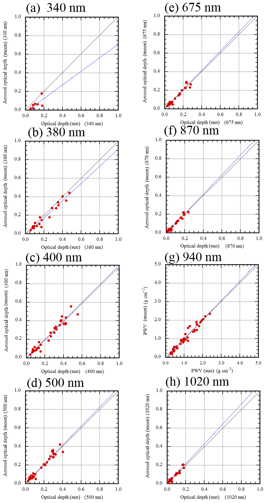
Figure 14 Scatter plot of the aerosol optical depth (precipitable water vapor) from the Sun and the moon: (a) 340 nm AOD, (b) 380 nm AOD, (c) 400 nm AOD, (d) 500 nm AOD, (e) 675 nm AOD, (f) 870 nm AOD, (g) 940 nm PWV, and (h) 1020 nm AOD.

Figure 14 shows a scatter plot of the AOD at the wavelengths of 340, 380, 400, 500, 675, 870, and 1020 nm, and the PWV from the 940 nm channel. Table 9 shows the results of the comparison between the AOD (PWV) from the Sun and from the moon (the contents of Table 9 are the same as Table 4 except for the AOD (PWV) from the Sun and the moon).

Table 9 Same as Table 4 except for the AOD (PWV) from the Sun and the moon.

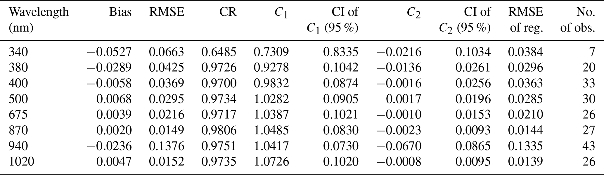
C₁ and C₂: coefficients of the regression line (${\mathit{\tau }}_{\mathrm{Moon}}=C_{\mathrm{1}}\cdot {\mathit{\tau }}_{\mathrm{Sun}}+C_{\mathrm{2}}$, ${\mathrm{PWV}}_{\mathrm{Moon}}=C_{\mathrm{1}}\cdot {\mathrm{PWV}}_{\mathrm{Sun}}+C_{\mathrm{2}}$).

The biases at wavelengths of 340 and 380 nm are relatively large, 0.05 and 0.03, respectively, but the biases at other wavelengths are 0.007 or less. The bias and RMSE of the PWV are 0.02 and 0.14, respectively, which are comparable to those from the comparison with POM-02 and the radiosonde or GPS. The correlation coefficient is high for all wavelengths; 0.65 at a wavelength of 340 nm, and 0.97 or higher at other wavelengths. Furthermore, the 95 % confidence interval of the slope value of the regression line includes 1, and the 95 % confidence interval of the intercept value includes 0. That is, the regression line is not different from a straight line with a slope of 1 and zero intercept at the 95 % confidence level. From these facts, the AOD and PWV retrieved using the moon as the light source are considered to be the same as those retrieved using the Sun as the light source at the 95 % confidence level.

6.4 Comparison between AERONET and POM-02

There is an AERONET observation site at MLO. In the nighttime, the AODs at wavelengths of 500, 675, 870, and 1020 nm, and the PWV can be compared. In addition to these channels, the AOD at wavelengths of 340, 380, and 1627 nm can be compared in the daytime. The AERONET data used here are level 2.0 in the daytime and level 1.5 in the nighttime. There were no level 2.0 nighttime data. AERONET level 1.5 are cloud-screened data but may not have had the final calibration applied. Thus, these data are not quality assured. AERONET level 2.0 has pre- and post-field calibration applied, cloud-screened, and quality-assured data (see the AERONET homepage; https://aeronet.gsfc.nasa.gov/, last access: 2 December 2019). The nighttime comparison in this paper uses the AERONET data without quality assurance.

Figure 15 shows a scatter plot of the AERONET and POM-02 AOD (PWV). The blue (red) symbols show the daytime (nighttime) data. Both the daytime and the nighttime data are overlaid: the AOD at wavelengths of 500, 675, 870, 1020 nm, and the PWV from the 940 nm channel. The plotted data are the 15 min averages. The number of measurements for POM-02 in a 15 min interval is 10 to 16, and that for AERONET is 1 to 6. Only POM-02 data showing small variations were selected; standard deviation/average is less than 0.1 or standard deviation is less than 0.02.

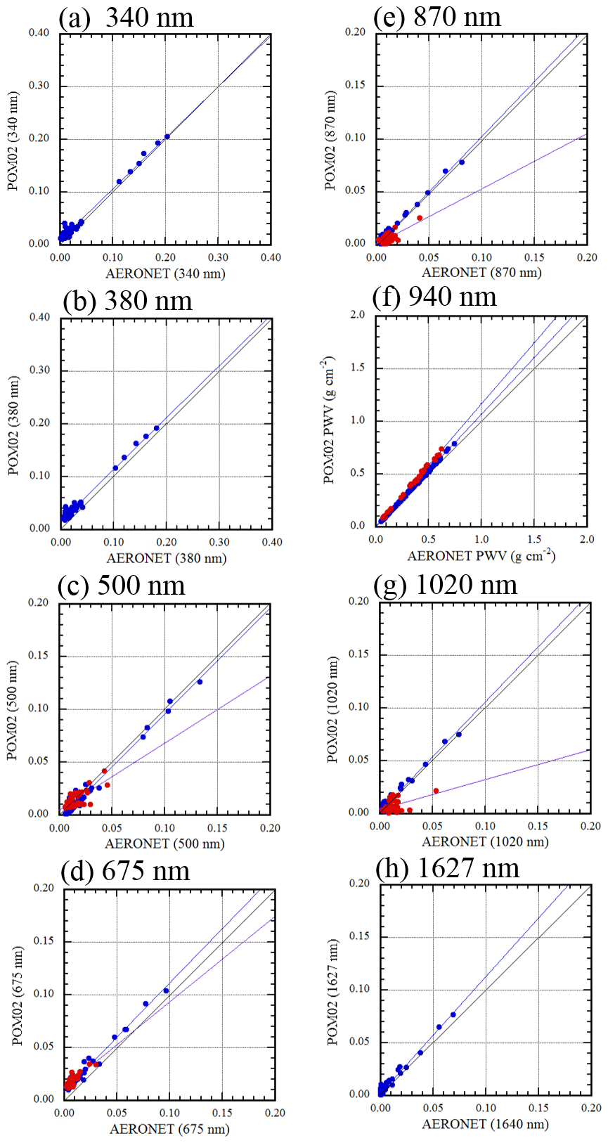
Figure 15 Scatter plot of AERONET and POM-02 aerosol optical depth (precipitable water vapor). Daytime (nighttime) measurements are indicated by a red (blue) symbol: (a) 340 nm AOD, (b) 380 nm AOD, (c) 500 nm AOD, (d) 675 nm AOD, (e) 870 nm AOD, (f) 940 nm PWV, (g) 1020 nm AOD, and (h) 1627 nm AOD.

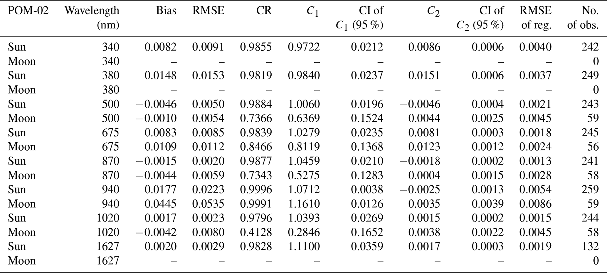
Table 10 shows the results of the comparison between the AERONET and POM-02 aerosol optical depth (precipitable water vapor); Table 10 is the same as Table 4 except for AERONET and POM-02 aerosol optical depth (precipitable water vapor). The values at 940 nm are the precipitable water vapor.

Table 10 Same as Table 4 except for the AERONET and POM-02 aerosol optical depth (precipitable water vapor).

In the daytime, from Fig. 15, it can be seen that the differences between AERONET and POM-02 AOD (PWV) are small. The 95 % confidence interval for the slope of the regression line does not necessarily include 1, but the slope value is nearly 1: between 0.97 and 1.11. The 95 % confidence interval for the intercept of the regression line does not necessarily include 0, but the magnitude of the intercept is 0.01 or less except for the 380 nm channel (0.015). The same can be said for the PWV of the 940 nm channel. In addition, the bias and RMSE are less than 0.01 except for the 380 nm channel (0.015), and those for the PWV at 940 nm are 0.018 and 0.022, respectively. Considering that the accuracy of the calibration constant is 0.5 % to 1 %, these values seem reasonable. Therefore, it can be inferred that in the daytime, POM-02 can measure the AOD (PWV) with the same level of accuracy as AERONET.

In the nighttime, the atmosphere observed at MLO was pristine, and most of the AODs at 500, 675, 870, and 1020 nm were below 0.02. Considering that the accuracy of the calibration constant is 0.5 % to 1 %, it is difficult to compare the AODs of AERONET and POM-02. In the nighttime, the slope of the regression line deviates from 1 at several wavelengths, but the bias and the RMSE are less than about 0.01. Therefore, the difference between AERONET and POM-02 is small. The slopes of the regression line for the PWV of 940 nm channel in the daytime and the nighttime are 1.07 and 1.16, respectively. Thus, the daytime and nighttime values differ. In the results of Sect. 6.3, there is almost no difference between the daytime and nighttime values. Therefore, this difference may be due to the lack of quality control in the nighttime data.

7 Summary and conclusion

Aerosol data are often estimated using the solar direct irradiance and the solar scattered radiance. Therefore, the majority of data on aerosol properties are obtained using daytime measurements, and there are few data available on aerosol characteristics at night. In order to estimate the aerosol optical depth (AOD) and the precipitable water vapor (PWV) during the nighttime using the moon as a light source, POM-02 (Prede Ltd., Japan), which is used to estimate aerosol characteristics during the daytime, was modified.

The current version of POM-02 has the ability to measure the direct irradiance from the moon for some channels in the visible and near-infrared wavelength region without requiring modification. Several modifications were made to also be able to measure the AOD during the nighttime and expand the measurement ranges.

The amplifier was adjusted so that POM-02 could measure up to about $\mathrm{5}\times {\mathrm{10}}^{-\mathrm{13}}$ A, allowing the lunar direct irradiance to be measured in the wavelength range of 340 to 1020 nm.

In order to track the moon based on the calculated value, the simplified formula by Nagasawa (1981) was incorporated into the firmware.

A position sensor with a four-quadrant detector is used to adjust the tracking of the Sun and the moon. In order to adjust the tracking of the moon, a position sensor incorporating a new electronic circuit to amplify the signal and new software to process the signal data were developed. The new position sensor can be used to track both the Sun and the moon.

The calibration constant was determined by using the Langley method. The measurements of the solar and lunar direct irradiance were conducted at the NOAA/MLO during the period from 28 September to 7 November 2017. Assuming that the correct lunar reflectance is proportional to the ROLO reflectance, the calibration constant for the lunar direct irradiance was determined by using the Langley method. The calibration by the Langley method was successfully performed.

The ratio of the calibration constant for the moon to that of the Sun was often greater than 1, where the ratio is a coefficient for correcting the ROLO reflectance and includes a smoothing factor. This ratio shows the error of the ROLO irradiance model. The value of the ratio was 0.95 to 1.18 in the visible and near-infrared wavelength region. This means that the ROLO model often underestimates the reflectance. In addition, this ratio depended on the phase angle: when the phase angle was small (near the full moon), the ratio was small, and as the phase angle became larger, the ratio increased. In this study, this ratio was approximated by the quadratic equation of the phase angle. By using this approximation, the reflectance of the moon can be calculated to within an accuracy of 1 % or less.

The continuous measurement of POM-02 was conducted at JMA/MRI from January 2018 to May 2018 and the AOD and PWV were estimated. In order to validate the estimates of the AOD and PWV, we compared them with the AOD and PWV obtained by independent methods. The AOD was compared with the AOD (532 nm) estimated from NIES/HSRL, and the PWV was compared with the PWV from a radiosonde and GPS. In addition, the continuity of the AOD (PWV) before and after sunrise and sunset at Tsukuba was examined, and the AOD (PWV) of AERONET and that of POM-02 at MLO were compared.

Concerning the AOD, there were sometimes systematic differences between NIES/HSRL and POM-02. The cause of the systematic differences seems to be that NIES/HSRL assumes a constant extinction coefficient at altitudes of less than 500 m. The slopes of the linear regression lines during the daytime and nighttime could not be said to be equivalent at the 95 % confidence level, but the scatter diagrams of the daytime and nighttime were almost overlapping.

Concerning the PWV, the slopes of the linear regression lines during the daytime and nighttime were equivalent at the 95 % confidence level in the comparisons between the PWV from POM-02 and the radiosonde and in the comparison between the PWV from POM-02 and GPS. Furthermore, the scatter diagrams of the daytime and the nighttime data were almost overlapping.

In addition, the comparison of the AOD (PWV) before and after sunrise and sunset showed that the AOD and PWV retrieved using the moon as the light source are the same as those retrieved using the Sun as the light source at the 95 % confidence level.

The comparison of the AOD (PWV) between AERONET and POM-02 was performed using the data taken during the calibration measurements. The comparison in the daytime showed that POM-02 can measure AOD (PWV) with the same accuracy as AERONET. The comparison in the nighttime showed that the difference in the AOD between AERONET and POM-02 was small. However, since there were a lot of optically thin data and AERONET data are not quality assured, we cannot make a definite conclusion.

From these facts, the daytime and nighttime AOD (PWV) measurements are statistically almost equivalent. The AODs (PWVs) during the daytime and nighttime for POM-02 are presumed to have the same degree of precision and accuracy within the measurement uncertainty.

The accuracy of the nighttime calibration constant is lower than that for the daytime. The measurement S∕N in the nighttime is also worse than that in daytime. Considering these facts, even if there is no statistically significant difference, the magnitude of the error in the AOD (PWV) during the nighttime is not always the same as that during the daytime.

In this study, the calibration was performed using about 40 d of data including two full-moon days. As a result, it was found that there was an error in the reflectance of the ROLO irradiance model. In the future, it is necessary to accumulate more data for calibration and to reduce the error of the ROLO irradiance model. It is said that the ROLO model can be applied over a phase angle range of about 90^∘. POM-02 has the ability to measure the direct lunar irradiance up to a phase angle range of about 120^∘. It is necessary to expand the ROLO irradiance model so that it can be applied to larger phase angles.

It is now possible to estimate the aerosol optical depth during the nighttime. It is necessary to promote the adoption of this system in the existing observation network. After that, the data obtained by using this instrument can be used to better understand nighttime aerosol behavior, for the validation of aerosol transport models, and as input data in assimilation systems.

Appendix A

The smoothed ROLO reflectance ${\stackrel{\mathrm{̃}}{A}}_{\mathrm{ROLO}}$ can be obtained by the procedure described in Kieffer and Stone (2005).

The calculated reflectance $A_{\mathrm{ROLO}}(g,\mathrm{\Phi },\mathit{\theta },\mathit{\varphi })$ at the 32 ROLO wavelengths for a specific geometric configuration $(g=\mathrm{7}{}^{\circ },\mathrm{\Phi }=\mathrm{7}{}^{\circ },\mathit{\theta }=\mathrm{0},\mathit{\varphi }=\mathrm{0})$ is fitted to a composite spectrum of the samples obtained by the Apollo 16 mission with a linear equation of wavelength λ.

$$\begin{array}{}\text{(A1)}& A_{\mathrm{Apollo}}=(a+b\mathit{\lambda })A_{\mathrm{ROLO}}(\mathrm{7},\mathrm{7},\mathrm{0},\mathrm{0}),\end{array}$$

where A_Apollo is the composite laboratory reflectance spectrum for the Apollo samples of soil (95 %) (Apollo 16 sample 62231; Pieters, 1999) and breccia (5 %) (Apollo 16 sample 67455; Pieters and Mustard, 1988).

The Apollo sample 62231 spectrum is available at http://www.planetary.brown.edu/pds/AP62231.html (last access: 2 December 2019). The Apollo sample 67455 spectrum is shown in Fig. 8 in the paper of Pieters and Mustard (1988).

The values of the coefficients a and b are not shown in Kieffer and Stone (2005) but were determined here with the least-squares method as follows:

$$\begin{array}{ll}{\displaystyle }a& {\displaystyle }=\mathrm{1.640875}\\ {\displaystyle }b& {\displaystyle }=-\mathrm{1.192034}\times {\mathrm{10}}^{-\mathrm{4}}\\ {\displaystyle },\end{array}$$

where the unit of the wavelengths is nanometers.

By dividing A_Apollo by a+bλ, the smoothed ROLO reflectance for a specific geometric configuration ${\stackrel{\mathrm{̃}}{A}}_{\mathrm{ROLO}}(\mathrm{7},\mathrm{7},\mathrm{0},\mathrm{0})$ can be obtained.

$$\begin{array}{}\text{(A2)}& {\stackrel{\mathrm{̃}}{A}}_{\mathrm{ROLO}}(\mathrm{7},\mathrm{7},\mathrm{0},\mathrm{0})=A_{\mathrm{Apollo}}/(a+b\mathit{\lambda })\end{array}$$

The smoothed ROLO reflectance ${\stackrel{\mathrm{̃}}{A}}_{\mathrm{ROLO}}(g,\mathrm{\Phi },\mathit{\theta },\mathit{\varphi })$ for any viewing geometry is given by the following equation:

$$\begin{array}{}\text{(A3)}& \begin{array}{rl}{\stackrel{\mathrm{̃}}{A}}_{\mathrm{ROLO}}& ={\displaystyle \frac{{\stackrel{\mathrm{̃}}{A}}_{\mathrm{ROLO}}(\mathrm{7},\mathrm{7},\mathrm{0},\mathrm{0})}{A_{\mathrm{ROLO}}(\mathrm{7},\mathrm{7},\mathrm{0},\mathrm{0})}}{A}_{\mathrm{ROLO}}(g,\mathrm{\Phi },\mathit{\theta },\mathit{\varphi })\\ & =F_C{A}_{\mathrm{ROLO}}(g,\mathrm{\Phi },\mathit{\theta },\mathit{\varphi }),\end{array}\end{array}$$

where $F_C={\stackrel{\mathrm{̃}}{A}}_{\mathrm{ROLO}}(\mathrm{7},\mathrm{7},\mathrm{0},\mathrm{0})/A_{\mathrm{ROLO}}(\mathrm{7},\mathrm{7},\mathrm{0},\mathrm{0})$.

The values of F_C are dependent on the interpolation method of the reflectance table and the accuracy of the values read from the figure. The smoothed and adjusted spectrum ${\stackrel{\mathrm{̃}}{A}}_{\mathrm{ROLO}}(\mathrm{7},\mathrm{7},\mathrm{0},\mathrm{0})$ is shown in Fig. A1. The values of F_C determined by the authors are shown in Table A1 and Fig. A2.

Figure A1 Coefficients for smoothing at the ROLO 32 wavelength.

Figure A2 ROLO smoothed and adjusted reflectance.

Table A1 Coefficients for smoothing at the ROLO 32 wavelength.