A neural network radiative transfer model approach applied to the Tropospheric Monitoring Instrument aerosol height algorithm

To retrieve aerosol properties from satellite measurements of the oxygen A-band in the near-infrared, a line-by-line radiative transfer model implementation requires a large number of calculations. These calculations severely restrict a retrieval algorithm's operational capability as it can take several minutes to retrieve the aerosol layer height for a single ground pixel. This paper proposes a forward modelling approach using artificial neural networks to speed up the retrieval algorithm. The forward model outputs are trained into a set of neural network models to completely replace line-by-line calculations in the operational processor. Results comparing the forward model to the neural network alternative show an encouraging outcome with good agreement between the two when they are applied to retrieval scenarios using both synthetic and real measured spectra from TROPOMI (TROPOspheric Monitoring Instrument) on board the European Space Agency (ESA) Sentinel-5 Precursor mission. With an enhancement of the computational speed by 3 orders of magnitude, TROPOMI's operational aerosol layer height processor is now able to retrieve aerosol layer heights well within operational capacity.

1 Introduction

Launched on 13 October 2017, The TROPOspheric Monitoring Instrument (Veefkind et al., 2012) on board the Sentinel-5 Precursor mission is the first of the satellite-based atmospheric composition monitoring instruments in the Sentinel mission of the European Space Agency. The aerosol layer height (ALH) retrieval algorithm (Sanders and de Haan, 2013; Sanders et al., 2015; Nanda et al., 2018a, b) is a part of TROPOMI's operational product suite, and is expected to be delivered in near-real time. The ALH (symbolised as z_aer) retrieval algorithm, operating within the near-infrared region in the oxygen A-band between 758 and 770 nm, exploits information on the heights of scattering layers derived from the absorption of photons by molecular oxygen – the amount of absorption indicates whether the scattering layer is closer to or farther from the surface; if the number of photons absorbed by oxygen is higher, it suggests a longer photon path length due to an aerosol layer present closer to the surface. This principle has been applied to cloud height algorithms such as FRESCO (Fast Retrieval Scheme for Clouds from the Oxygen A-band) by Wang et al. (2008), which use lookup tables to generate top-of-atmosphere (TOA) reflectances to compute cloud parameters. As clouds are such efficient scatterers of light, FRESCO can approximate scattering by cloud using a Lambertian model – this simplification works quite well for optically thick cloud layers. For aerosol layers, however, such calculations need to be carried out in much greater detail due to their weaker scattering properties. TROPOMI's ALH algorithm employs the DISAMAR (Determining Instrument Specifications and Methods for Atmospheric Retrievals) science code; DISAMAR uses the “Layer Based Orders of Scattering” (LABOS) radiative transfer model based on the doubling–adding method (de Haan et al., 1987), which calculates reflectances at the TOA and its derivatives with respect to aerosol layer height and aerosol optical thickness (τ). These calculations are carried out line-by-line, requiring calculations at 3980 wavelengths to generate these TOA reflectances within the oxygen A-band. Having computed the TOA reflectance spectra, aerosol layer heights are retrieved with optimal estimation (OE), an iterative retrieval scheme developed by Rodgers (2000) that incorporates a priori knowledge of retrieval parameters into their estimation. Such a retrieval scheme also provides a posteriori error estimations, which are important for assimilation models and diagnosing the retrieval results.

The ALH retrieval algorithm is computationally expensive, requiring several minutes to compute z_aer for a single ground pixel (Sanders et al., 2015). As near-real time processors need to consistently go through large volumes of data recorded by the satellite for the mission lifetime, TROPOMI's operational computation capability is much restricted. This is due to the fact that TROPOMI records approximately 1.4 million pixels within a single orbit where, on average, 50 000 pixels are typically identified as aerosol contaminated pixels (with a UV aerosol index, UVAI, value greater than 0.0) for retrieving aerosol layer height. This places a steep requirement on the computational infrastructure with respect to processing all possible pixels from a single orbit. The online radiative transfer model severely limits the ALH data product, processing only a small fraction of the total possible pixels within a single orbit while compromising the timeliness of the data delivery.

The bottleneck identified here is the large number of calculations that the forward model has to compute to retrieve information on weak scatterers such as aerosols. Several steps to circumvent this bottleneck exist, such as using correlated k distribution method to reduce the number of calculations (Hasekamp and Butz, 2008), using a lookup table to calculate forward model outputs, or entirely foregoing the forward model and directly retrieving z_aer from observed spectra using neural networks (Chimot et al., 2017, 2018). Studies by Sanders and de Haan (2016) have shown that the lookup table for reflectance alone measure up to 46 GB in size, and is perhaps a similar size or even larger for the derivatives. Chimot et al. (2017) describe an approach using a radiative transfer model to generate slant column densities of the O₂–O₂ band at 477 nm from Ozone Monitoring Instrument (OMI) measurements for different aerosol optical depths (among other input parameters) to train several artificial neural network models that directly retrieve aerosol layer height. Operationally, their neural network models use the MODIS aerosol optical depth at 550 nm and retrieved OMI slant column densities, thereby entirely foregoing line-by-line calculations and significantly speeding the retrieval algorithm up. The trained neural network models directly retrieved aerosol layer heights from spectra measured by OMI on board the NASA Aura mission, without using line-by-line calculations or an iterative estimation step such as OE (Chimot et al., 2018). A similar example of retrievals is the ROCINN (Retrieval of Cloud Information using Neural Networks) cloud algorithm developed by Loyola (2004) which uses neural networks to compute convolved reflectance spectra to retrieve cloud properties. These retrievals show the exploitable capabilities of artificial neural networks in the context of retrieving atmospheric properties from oxygen absorption bands.

The studies of Chimot et al. (2018) and Loyola et al. (2018) bring to light the efficacy of artificial neural networks in the satellite remote sensing of oxygen absorption bands for retrieving properties of scattering species in the atmosphere. This paper discusses a method inspired by Chimot et al. (2017) and Loyola (2004) to retrieve the aerosol layer height from oxygen A-band measurements by TROPOMI. While Chimot et al. (2017) directly retrieved aerosol layer heights from their neural network models, the operational algorithm in this paper utilises neural networks to calculate top-of-atmosphere radiances in the forward model. This is subsequently used by an optimal estimation scheme to retrieve aerosol layer heights. Similarly while Loyola (2004) derived top-of-atmosphere sun-normalised radiances only for their cloud property retrieval algorithm, the method in this paper has dedicated neural network models that calculate the Jacobian as well as the top-of-atmosphere sun-normalised radiances. By reducing the time consumed for calculating forward model outputs, the computational efficiency of TROPOMI's aerosol layer height retrieval algorithm can be significantly improved.

Section 2 introduces the operational aerosol layer height algorithm and discusses the line-by-line forward model. The neural network forward model approach is detailed in Sect. 3, and its verification on a test data set is discussed in same section. This approach is then applied to various test cases using synthetic and real TROPOMI spectra (Sect. 4) before conclusions are given in Sect. 5.

2 The TROPOMI aerosol layer height retrieval algorithm

The TROPOMI aerosol layer height is one of the many algorithms that exploit vertical information on scattering aerosol species in the oxygen A-band (Timofeyev et al., 1995; Gabella et al., 1999; Corradini and Cervino, 2006; Pelletier et al., 2008; Dubuisson et al., 2009; Frankenberg et al., 2012; Sanghavi et al., 2012; Wang et al., 2012; Sanders and de Haan, 2013; Hollstein and Fischer, 2014; Sanders et al., 2015; Geddes and Bösch, 2015; Sanders and de Haan, 2016; Colosimo et al., 2016; Davis et al., 2017; Xu et al., 2017; Nanda et al., 2018b; Zeng et al., 2018). These methods invert a forward model that describes the atmosphere, to compute the height of the scattering layer. This section discusses the set-up of the TROPOMI ALH retrieval algorithm, which consists of the inversion of a forward model representing the atmosphere using optimal estimation as the retrieval method, and a description of the forward model.

2.1 The retrieval method

The cost function χ² represents the departure of the modelled reflectance F(x) from the observed reflectance y constrained by the measurement error covariance matrix S_ϵ, and is defined as

$$\begin{array}{}\text{(1)}& \begin{array}{rl}{\mathit{\chi }}^{\mathrm{2}}& ={\left[\mathit{y}-\mathit{F}\mathbf{\left(}\mathit{x}\mathbf{\right)}\right]}^{\mathrm{T}}{\mathbf{S}}_{\mathit{ϵ}}^{-\mathrm{1}}\left[\mathit{y}-\mathit{F}\mathbf{\left(}\mathit{x}\mathbf{\right)}\right]\\ & +{\left(\mathit{x}-{\mathit{x}}_{\mathrm{a}}\right)}^{\mathrm{T}}{\mathbf{S}}_{\mathrm{a}}^{-\mathrm{1}}\left(\mathit{x}-{\mathit{x}}_{\mathrm{a}}\right).\end{array}\end{array}$$

Minimising this cost function for a particular z_aer and τ (the elements of the state vector x to be retrieved and fitted) gives us the final retrieval product. This definition of the cost function is unique to OE, as it is constrained with a priori knowledge of the state vector x (represented by x_a) and the a priori error covariance matrix S_a. In the TROPOMI ALH processor's OE framework, the a priori state vector is fixed at specific values, usually 200 hPa above the surface for z_aer and 1.0 for τ at 760 nm. The a priori error of the z_aer is fixed at 500 hPa, and the a priori error for τ is fixed at 1.0, to allow freedom for the variables in the estimation (this also reduces the impact of the a priori on the retrieval). The forward model is employed to simulate the measured reflectance spectrum with model parameter x with

$$\begin{array}{}\text{(2)}& F\left(\mathit{x}\right)\left(\mathit{\lambda }\right)={\displaystyle \frac{\mathit{\pi }I\left(\mathit{\lambda }\right)}{{\mathit{\mu }}_{\mathrm{0}}{E}_{\mathrm{0}}\left(\mathit{\lambda }\right)}},\end{array}$$

where I and E₀ represent the Earth radiance and solar irradiance respectively, with the cosine of the solar zenith angle (θ₀) denoted by μ₀. As the forward model is non-linear, a Gauss–Newton iteration is employed to the updated state vector as follows:

$$\begin{array}{}\text{(3)}& \begin{array}{rl}{\mathit{x}}_{\mathit{i}\mathbf{+}\mathbf{1}}& ={\mathit{x}}_{\mathrm{a}}+{\left[{\mathbf{K}}_i^{\mathrm{T}}{\mathbf{S}}_{\mathit{ϵ}}^{-\mathrm{1}}{\mathbf{K}}_i+{\mathbf{S}}_{\mathrm{a}}^{-\mathrm{1}}\right]}^{-\mathrm{1}}{\mathbf{K}}_i^{-\mathrm{1}}{\mathbf{S}}_{\mathit{ϵ}}^{-\mathrm{1}}\\ & \left[\mathit{y}-\mathit{F}\mathbf{\left(}\mathit{x}\mathbf{\right)}+{\mathbf{K}}_i\left({\mathit{x}}_i-{\mathit{x}}_{\mathrm{a}}\right)\right],\end{array}\end{array}$$

where K_i is the matrix of derivatives (Jacobian) of the reflectance with respect to the state vector parameters at the current iteration i. The derivatives are calculated semi-analytically similar to the method described by Landgraf et al. (2001). The nth iterative estimate is convergent to a solution if the relative changes in the state vector are less than the expected precision (usually fixed at a certain value). The retrieval is said to be “failed” if the number of iterations exceeds the maximum number of iterations (usually set to 12) or the state vector parameters are projected outside the respective boundary conditions. Retrieval errors are derived from the a posteriori error covariance matrix $\widehat{\mathbf{S}}$, which is computed as

$$\begin{array}{}\text{(4)}& \widehat{\mathbf{S}}={\left[{\mathbf{K}}^{\mathrm{T}}{\mathbf{S}}_{\mathit{ϵ}}^{-\mathrm{1}}\mathbf{K}+{\mathbf{S}}_{\mathrm{a}}^{-\mathrm{1}}\right]}^{-\mathrm{1}}.\end{array}$$

2.2 The DISAMAR forward model and its many simplifications of atmospheric properties

Optimal estimation iteratively simulates TOA radiance spectra until the convergence of χ² (Eq. 1). For this, DISAMAR computes reflectances at a high-resolution wavelength grid. The computed high-resolution reflectances are combined with a reference solar spectrum derived from Chance and Kurucz (2010) to obtain a high-resolution Earth radiance. The high-resolution Earth radiance and the solar spectrum are convolved with the instrument spectral response function to obtain the Earth radiance and solar irradiance spectrum in the instrument's wavelength grid, before finally computing the reflectance spectrum in the instrument grid using Eq. (2). It is important to note that the steps of including the reference solar spectrum to compute reflectances in the instrument's wavelength grid are not undertaken by the neural network algorithm. The neural network aerosol layer height retrieval algorithm directly convolves the reflectance. The difference between including and excluding a reference spectrum in the convolution process results in differences in the order of 4 % to 5 % around 762 and 766 nm. Further on in this paper, a direct comparison between DISAMAR retrievals of the aerosol layer height and retrievals with the neural network algorithm is provided.

Reflectances are calculated by accounting for scattering and absorption of photons from their interactions with aerosols, the surface, and molecular species. Molecular scattering of photons in the oxygen A-band is described by Rayleigh scattering, and absorption is described by photon-induced magnetic dipole transition between $b^{\mathrm{1}}{\mathrm{\Sigma }}_g^{+}\leftarrow X^{\mathrm{3}}{\mathrm{\Sigma }}_g^{-}(\mathrm{0},\mathrm{0})$ electric potential levels of molecular oxygen and collision-induced absorption between O₂–O₂ and O₂–N₂. The total influence of the oxygen A-band on the TOA reflectance is described by its extinction cross-section, which is the sum of the three aforementioned contributions. As the vertical distribution of oxygen is exactly known, the extinction cross-section can be exploited to retrieve z_aer from satellite measurements of the oxygen A-band. For this, DISAMAR calculates absorption (or extinction) cross-sections at 3980 wavelengths within the range of 758–770 nm.

To reduce the number of calculations, various atmospheric properties are simplified. As the Rayleigh optical thickness is low at 760 nm, DISAMAR only computes the monochromatic component of light by calculating the first element of the Stoke's vector. The exclusion of higher-order Stoke's vector elements of the radiation fields has not shown to be a significant source of error (Sanders and de Haan, 2016).

Calculating the influence of rotational Raman scattering (RRS) is also ignored, as it is a computationally expensive step. While this exclusion of RRS is not advised by the literature (Vasilkov et al., 2013; Sioris and Evans, 2000), preliminary experiments by Sanders and de Haan (2016) have ascertained that the errors in the retrieved aerosol layer height resulting from ignoring the RRS of the oxygen A-band in the forward model are significantly smaller than the effect of other model errors such as errors due to incorrect surface albedo. Therefore, RRS has historically not been simulated in the forward model of the Royal Netherlands Meteorological Institute (KNMI) aerosol layer height retrieval algorithm. The atmosphere is assumed to be cloud-free, which is a required simplification as the retrieval of z_aer in the presence of clouds is still challenging (Sanders et al., 2015); therefore, z_aer retrieval is only performed for pixels which are unlikely to contain clouds. Compared with totally cloud-free scenes, errors in retrieved z_aer are large for cloud-free scenes containing undetected optically thin cirrus clouds (Sanders et al., 2015). The fraction of the pixel containing aerosols is assumed to be 100 %, which further simplifies the representation of aerosols within the atmosphere.

Perhaps the largest simplification of the atmosphere lies in model's description of aerosols, assumed to be distributed in a homogeneous layer at a height z_aer with a 50 hPa thickness, a fixed aerosol optical thickness (τ), and a single scattering albedo (ω) of 0.95 (so, scattering aerosols). A Henyey–Greenstein model (Henyey and Greenstein, 1941) with an asymmetry parameter g value of 0.7 is used to parameterise the aerosol scattering phase function, which is one of the widely used approximations. These fixed aerosol optical properties have been derived from AERONET data and tested by Sanders et al. (2015), who retrieved z_aer from GOME-2 spectra to show that the algorithm is robust with respect to fixed aerosol model parameters such as the single scattering albedo and the Henyey–Greenstein phase function asymmetry parameter. The surface is assumed to be an isotropic reflector with a brightness described by its Lambertian equivalent reflectivity (LER). This is also an important simplification, requiring less computations over other surface models such as a bi-directional reflectance model. Although the forward model is capable of including sun-induced chlorophyll fluorescence into the retrieval, it is currently being considered for a future implementation of TROPOMI's operational ALH retrieval algorithm. Lastly, the atmosphere is spherically corrected for incoming solar radiation and remains plane-parallel for outgoing Earth radiance.

These simplifications in the DISAMAR forward model are a necessity for the line-by-line aerosol layer height algorithm, owing to its slow computational speed. The speed-up of forward model simulation encourages an increase in the complexity of the simulation assumptions.

2.3 Application to TROPOMI

TROPOMI's near-infrared (NIR) spectrometer records data between 675 and 775 nm, spread across two bands: band 5 contains the oxygen B-band and band 6 contains the oxygen A-band. The spectral resolution, which is described by the full width at half maximum (FWHM) of the instrument spectral response function (ISRF), is 0.38 nm with a spectral sampling interval of 0.12 nm. The spatial resolution is around 7 km×3.5 km for bands 5 and 6. Initial observations from the TROPOMI NIR spectrometer show a signal-to-noise ratio (SNR) of 3000 in the continuum before the oxygen A-band. The instrument polarisation sensitivity is reduced to below 0.5 % by adopting the technology of the OMI polarisation scrambler (Veefkind et al., 2012; Levelt et al., 2006). DISAMAR utilises TROPOMI's swath-dependent ISRFs to convolve I(λ) and E₀(λ) into I(λ_i) and E₀(λ_i) in the instrument's spectral wavelength grid respectively, after which the modelled reflectance is calculated using Eq. (2).

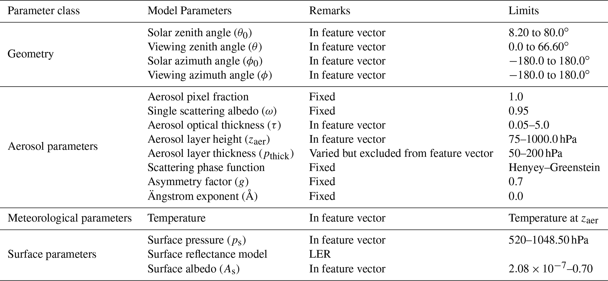
Input parameters required by the TROPOMI ALH retrieval algorithm encompass satellite observations of the radiance and the irradiance, solar–satellite geometry, and a host of atmospheric and surface parameters required for modelling the interactions of photons within the Earth's atmosphere (see Table 1). Meteorological parameters are taken from ECMWF (European Centre for Medium-Range Weather Forecasts), including the temperature–pressure profile at 91 atmospheric levels (of which the surface is a part). The various geophysical parameters are interpolated to TROPOMI's ground pixels using nearest neighbour interpolation.

TROPOMI incorporates information from the VIIRS instrument to detect the presence of cirrus clouds in the measured scene (using a cirrus reflectance threshold of 0.01). This information is further combined with cloud fraction retrievals by the TROPOMI FRESCO algorithm (maximum cloud fraction of 0.6), and the difference between the scene albedo in the database in the UV band and the apparent scene albedo at the same wavelength calculated using a lookup table (if the difference is larger than 0.2, it suggests cloud contamination). A combination of these different cloud detection strategies results in the “cloud_warning” flag in the Level-2 TROPOMI ALH product. In this paper, however, we use a strict FRESCO cloud fraction filter of 0.2 to remove cloudy pixels.

Tilstra et al. (2017)

Table 1 Input parameters required for retrieving aerosol layer height using TROPOMI measured spectra.

Calculation of TOA reflectance and its derivatives with respect to z_aer, and τ in a line-by-line fashion takes approximately 40–60 s to complete on a computer equipped with Intel(R) Xeon(R) CPU E3-1275 v5 at a clock speed of 3.60 GHz. In an iterative framework such as the Gauss–Newton method, the retrieval of z_aer can take between three and six iterations depending on the amount of aerosol information available in the observed spectra, requiring several minutes to compute retrieval outputs for a specific scene. If these retrievals fail by not converging within the maximum number of iterations, the processor can waste up to 10 min on a pixel without retrieving a product. In order to compute DISAMAR's outputs more quickly, a neural network implementation is discussed in the next section.

3 The neural network (NN) forward model

Artificial neural networks consist of connected processing units, each individually producing an output value given a certain input value. The interaction of these individual processing units, also known as nodes (or neurons), enable the connecting network to map a set of inputs (also known as the input layer) to a set of outputs (also known as the output layer). The connections are known as weights and their values symbolise the strength of a connection between two nodes. As the nodes connect inputs to the outputs, higher values in a set of connecting weights represent a stronger influence of a particular parameter in the input layer over a particular parameter in the output layer. These weights are determined after training the neural network.

The training (or optimisation) of a neural network begins with a training data set containing many instances of input and output layer elements. As true values of the output layer for a given set of inputs are exactly known in the training data set, the biased output of the neural network calculated after using randomised, non-optimised weights can be easily calculated. These biases are called prediction errors, and are an essential element in the optimisation of the neural network weights. The mean squared error (MSE) between the true output and the calculated output is also called the loss function (henceforth annotated as Δ), which is synonymous with a cost function (Eq. 5),

$$\begin{array}{}\text{(5)}& \mathrm{\Delta }={\displaystyle \frac{\mathrm{1}}{n_{\mathit{\lambda }}}}\sum _{\forall \mathit{\lambda }}{\left({\text{nn}}_{\mathit{\lambda }}-o_{\mathit{\lambda }}\right)}^{\mathrm{2}}.\end{array}$$

Here λ is the wavelength, n_λ represents the number of elements in the output layer, nn_λ represents the calculated output for wavelength via forward propagation, and o_λ are the outputs in the training data set. The weights are updated using optimisers such as the “Adam” optimiser (adaptive moment estimation) by Kingma and Ba (2014) to minimise Δ, within set number of iterations.

3.1 The TROPOMI NN forward model for the ALH retrieval algorithm

The standard architecture of the NN-augmented operational aerosol layer height processor includes three neural network models for estimating top-of-atmosphere sun-normalised radiance, the derivative of the reflectance with respect to z_aer, and the same for τ. It is also possible to assign the neural network to compute the reflectance instead of the sun-normalised radiance – the results will not change. The definition of sun-normalised radiance used in this paper is the ratio of Earth radiance to solar irradiance. DISAMAR calculates derivatives with respect to reflectance, which is the sun-normalised radiance multiplied by the ratio of π and cosine of the solar zenith angle. All three neural network models share the same input model parameters. Optimising a single neural network model for all three forward model outputs is not necessary; the correlations between the input parameters and the different forward model outputs are different, which can complicate the optimisation of a general-purpose neural network. This paper, however, acknowledges modern developments in neural network optimisation techniques that now afford selectively when optimising a neural network for different tasks (Kirkpatrick et al., 2016; Wen and Itti, 2018).

The models are trained using the Python Tensorflow module (Abadi et al., 2015), and further implemented into an operational processor using the C++ interface to Tensorflow. These neural network models require training data containing DISAMAR input and output parameters and a connecting architecture that encompasses the input feature vector containing scene-varying model parameters, the number of hidden layers, the number of nodes in each hidden layer, and an activation function that maps the input to the final output layer containing DISAMAR outputs. In Tensorflow, the derivative of Δ with respect to the weights are computed using reverse-mode automatic differentiation, which computes numerical values of derivatives without the use of analytical expressions (Wengert, 1964).

The inputs for NN are collectively referred to as the feature vector. The parameters included in the feature vector are a very important factor deciding the performance of the neural network. The primary classes of model parameters (relevant to retrieving z_aer) that vary from scene to scene are solar–satellite geometry, aerosol parameters, meteorological parameters, and surface parameters (Table 2). The various aerosol parameters that are fixed from scene to scene are the aerosol single scattering albedo (ω), the asymmetry factor of the phase function, and the Ängstrom exponent, as they are also fixed in the line-by-line operational aerosol layer height processor. The scattering phase function of aerosols is currently limited to a Henyey–Greenstein model with a fixed g value of 0.7 to mimic DISAMAR. Surface pressure as well as the temperature–pressure profile are two important meteorological parameters relevant to retrieving z_aer. A difference between the DISAMAR and NN models is the definition of this temperature information in the input. DISAMAR requires the entire temperature–pressure profile of the atmosphere, whereas NN only uses the temperature at z_aer. Surface albedo is specified at 758 nm as well as 772 nm in DISAMAR, whereas it is only specified at 758 nm in the feature vector of NN. In general there is a greater scope to add detailed information in DISAMAR. However, DISAMAR has historically incorporated many simplifications in order to reduce computational time. The current NN model is developed with the aim of mimicking DISAMAR as much as possible, without including additional state vector elements into the retrieval, such as chlorophyll fluorescence, aerosol optical properties, cloud properties, and so on.

Table 2 Scene-dependent input model parameters for the NN model. See also Fig. 1 for a histogram of the input parameters. The solar–satellite geometry parameters are generated in combinations conforming to those encountered by TROPOMI's orbits.

3.2 Training the neural networks

As the NN forward model is specifically designed for TROPOMI, the solar–satellite geometry is selected to represent TROPOMI orbits for the training data. Meteorological parameters for the locations associated with these solar–satellite geometries are derived from the 2017 60-layer ERA-Interim reanalysis data (Dee et al., 2011), and aerosol and surface parameters are randomly generated within their physical boundaries. This training data generation strategy spans the entire set of TROPOMI solar and viewing angles as well as meteorological parameters.

Generally, the required training data size increases with increasing nonlinearity between input and output layers in a neural network – there is no specific method to accurately determine the required sample size before training. The number of spectra generated for the training set was determined by training different models with a different number of spectra in the training set ranging from 1000 to 600 000. In general it was observed that incorporating more data resulted in a better neural network model. In order to test the trained neural network model, 500 000 spectra were selected. Finding the most optimal neural network configuration requires testing the trained neural network model. To that end, the training data set was divided into a training–testing split, where the model was trained on the majority of the training data set and tested on the remaining minority. Once trained, the model was tested again on a test data set with 100 000 scenes outside of the training data set. These spectra were generated using DISAMAR with the model parameter ranges described in Table 2. Figure 1 plots the distribution of the input parameters necessary for training the neural network. The neural network model accepts solar azimuth and viewing azimuth angles separately; however, they are plotted together as the relative azimuth angle in Fig. 1 to save space. The generation of this training data set is by far the most time-consuming step as each DISAMAR run requires between 50 and 60 s to generate the synthetic spectra. Once the data have been generated, they are prepared for training the neural network models in NN. This is done by data normalisation, which is achieved by subtracting the mean of each of the training input and output parameters and dividing the difference by its standard deviation; this treatment of the data makes the learning process quicker by reducing the search space for the optimiser. The offset and scaling parameters are important, as the neural network computes outputs within this scaled range, which needs to be rescaled back to physical values. This training requires a few hours on an Intel(R) Xeon(R) CPU E3-1275 v5 at a clock speed of 3.60 GHz.

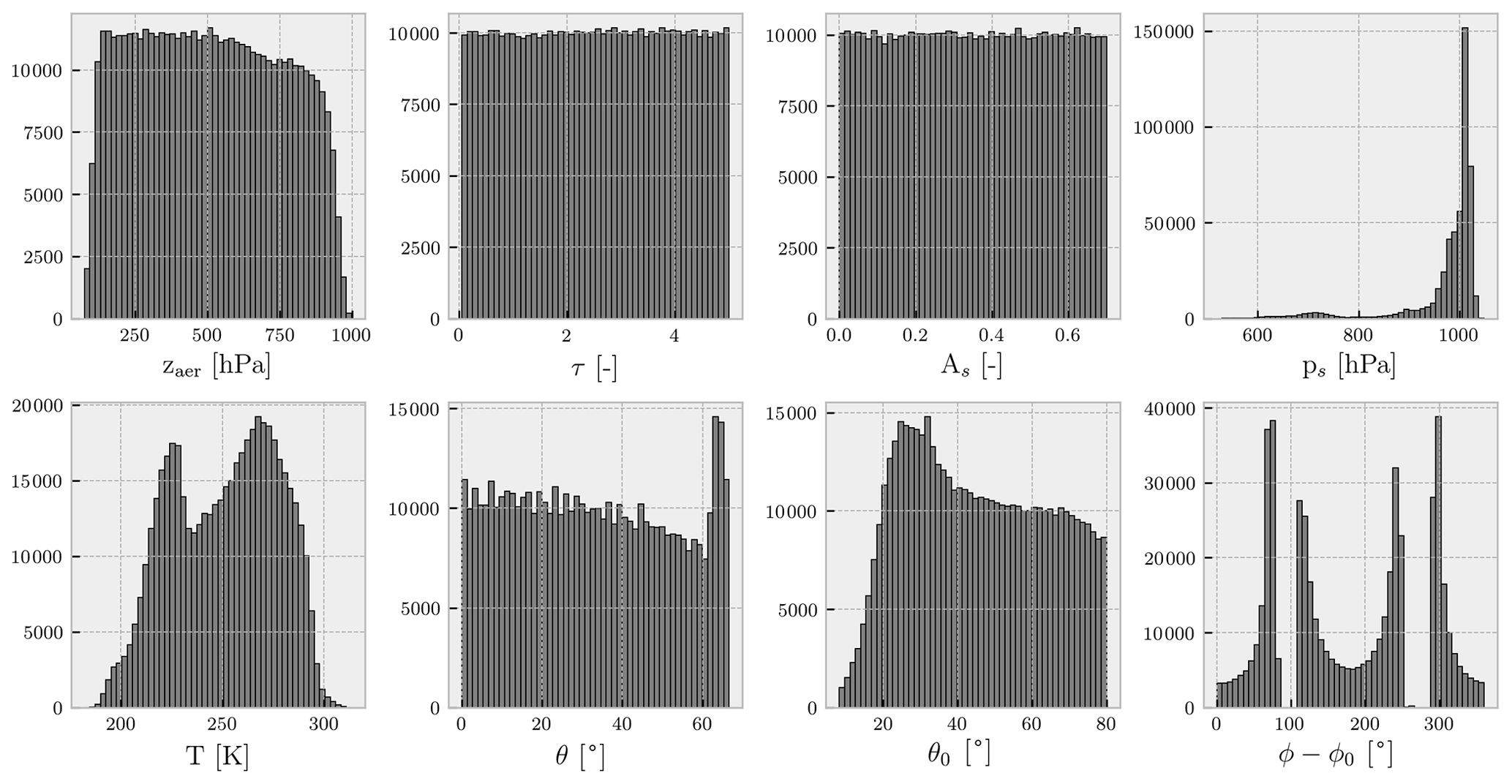
Figure 1 Histograms of the various input parameters for each of the neural network models in NN. Minimum and maximum values for each of the parameters are shown in Table 2.

The most optimal configurations for each of the three NN models are determined by the number of hidden layers, the number of nodes on each layer, and the chosen activation function for which the discrepancy between the modelled output for specific inputs and the truth (derived from DISAMAR) is minimal. The difference between the outputs calculated by DISAMAR and NN for these three models provides insight into their performance.

In order to test the most optimal number of layers, the most optimal number of nodes per layer, and the activation function, several neural network configurations were trained for 250 000 iterations and their summed losses (defined as Δ×n_λ) were compared to find out which configuration was best. Figure 2 plots the summed losses as a function of training iteration for different configurations.

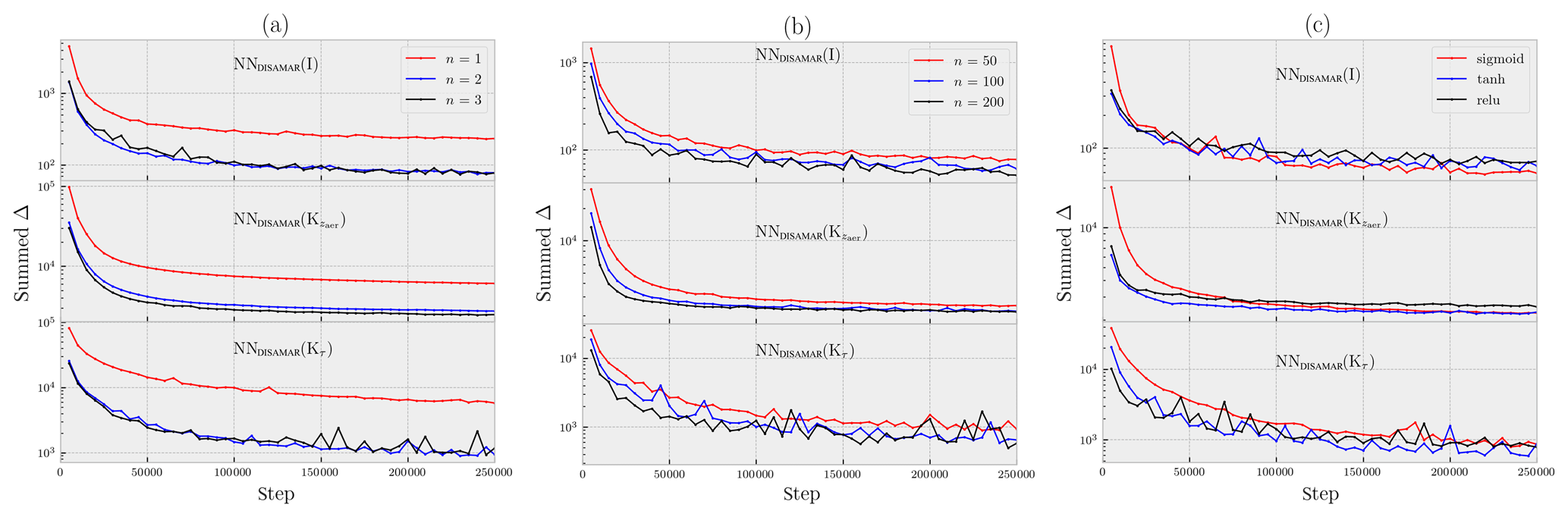
Figure 2 Summed loss as a function of training step for different neural network model configurations. (a) The neural network models have 50 nodes per layer with a sigmoid activation function. (b) The neural network models have two hidden layers with each node activated by the sigmoid function. (c) The neural network models have two hidden layers with 100 nodes for each layer.

To begin, with 50 nodes per hidden layer, three neural networks – one-layered, two-layered, and three-layered – for each of the three models were trained. The neural network models performed best with at least two hidden layers (Fig. 2a). For all three models, the two-layered versions show a similar summed loss to their three-layered alternatives, with the summed loss for the two-layered NN_DISAMAR(K_τ) showing more stability with training epoch. Therefore, a simpler two-layered architecture is chosen for all three models. Continuing on, three other architectures for each of the three models were chosen with 50, 100, and 200 nodes for each of the two hidden layers. The results showed that with more training steps, the choice of 100 nodes for each of the two layers was a good compromise between summed training loss and simplicity (Fig.  2b), especially for NN_DISAMAR(K_τ). Finally, going ahead with a two-layered architecture and 100 nodes for each layer, three activation functions – namely the sigmoid function, the hyperbolic tangent function (tanh), and the rectified linear unit (relu) function – were tested for each of the neural network models (Fig. 2c). In this case, while all functions converge to similar summed loss values by 250 000 iterations, the sigmoid function showed a good compromise between training loss and stability. Figure 3 gives a graphic representation of the neural network model.

Figure 3 Schematic of each of the three neural networks in NN. There are two hidden layers, each containing 100 nodes. z represents inputs for each of the nodes, whereas nn represents the inputs and outputs of the neural network.

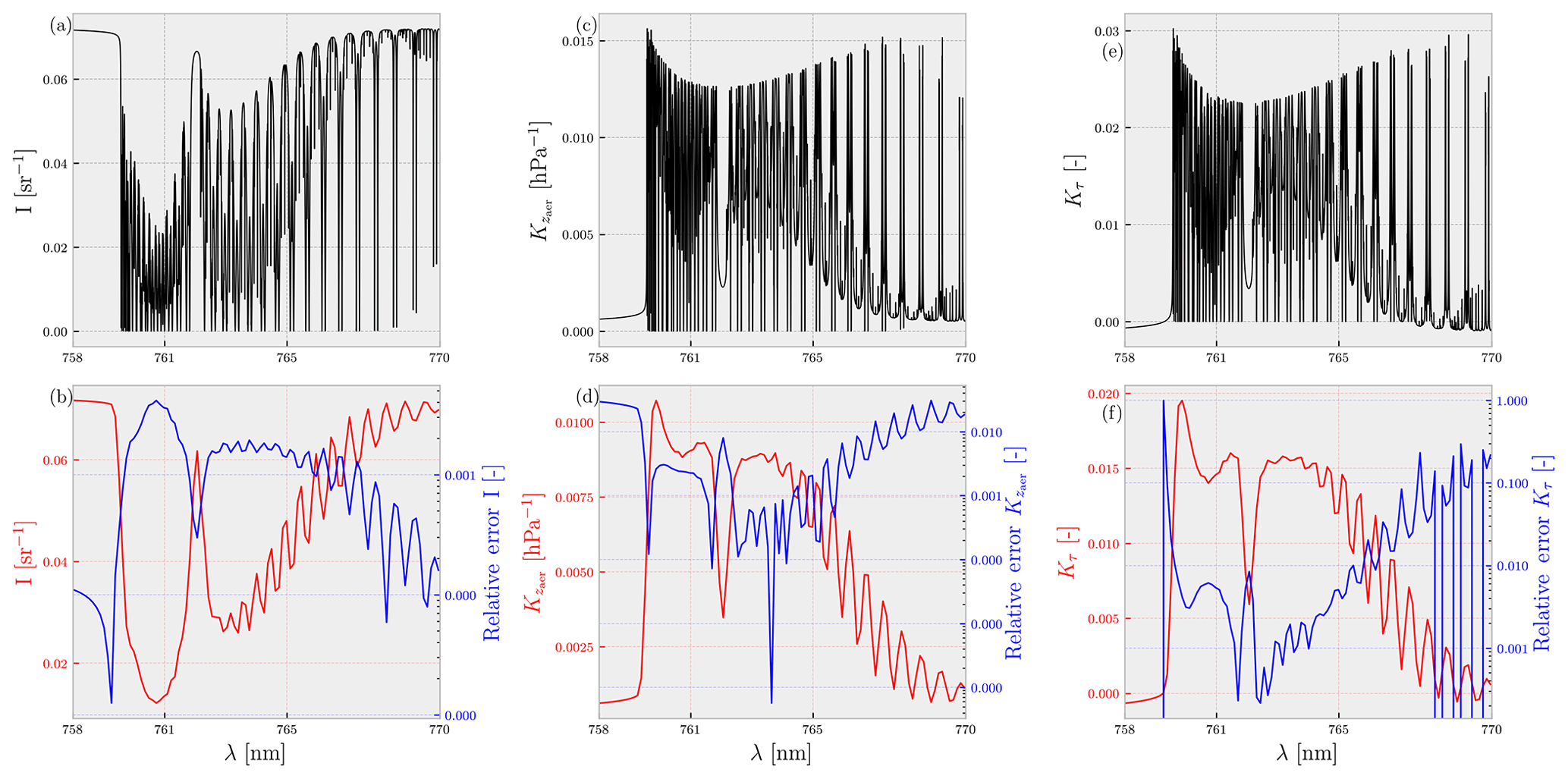
Figure 4 Performance of the finalised neural network. Panels (a), (c), and (e) represent the averaged output of each of the neural networks for surface albedo less than 0.4. Panels (b), (d), and (f) represent the convolved version of (a), (c), and (e) (plotted as the red line read from the left-hand y axis) and the convolved relative error (plotted in log scale) with the truth (plotted in blue and read from the right-hand y axis). The relative errors are computed as the absolute value of the difference (post-convolution) between the averaged true and averaged predicted spectra, divided by the averaged true spectra. Panels (a) and (b) represent the neural network computed sun-normalised radiances, panels (c) and (d) represent the same for the derivative of reflectance with respect to the aerosol layer height, and panels (e) and (f) represent the same with respect to the aerosol optical thickness.

The finalised configurations were then trained for 1 million iterations after which they were applied to the test data set to study prediction errors. Figure 4 plots the performance of each of the neural networks trained on the testing data set. An error analysis revealed that the trained neural networks were capable of calculating DISAMAR outputs with low errors, generally within 1 %–3 % of DISAMAR calculations. Averaged convolved errors of the neural network model for the sun-normalised radiance (NN_I) did not exceed 1 %. The neural network model for the derivative of the reflectance with respect to τ and z_aer perform well in general for parts of the spectrum with large oxygen absorption cross-sections, where the value of the derivatives are high (indicating a higher amount of information content from those specific wavelength regions). Errors in the deepest part of the R-branch between 759 and 762 nm and the P-branch between 752.50 and 765 nm do not exceed 3 % for ${\text{NN}}_{K_{\mathrm{zaer}}}$. The same can be said for ${\text{NN}}_{K_{\mathit{\tau }}}$, which displays errors of approximately 1 % in the same wavelength region. For wavelengths outside of the deepest parts of the R- and P-branch, the relative errors are large, and easily exceed 10 %. However, the relative errors are calculated as the absolute value of the difference between the true spectrum and the neural-network-calculated spectrum, divided by the true spectrum. These values can be very large when the value of the true spectrum is very small, which is the case for the derivatives outside the deepest part of the R- and P-branch. The consequences of these errors in a retrieval scenario from synthetic and real spectra are discussed in the following section.

4 Comparison between DISAMAR and NN aerosol layer height retrieval algorithms

To test the NN-augmented retrieval algorithm, we apply the generated NN models to synthetic test data and real data from TROPOMI and compare its retrieval capabilities to those of DISAMAR. The synthetic data were produced using the DISAMAR radiative transfer model; therefore, we expect the online radiative transfer retrievals to be generally better than the NN-based retrievals. The aerosol model utilised in the retrieval is the same at that in Sect. 2.2, using fixed parameters for aerosol single scattering albedo, aerosol layer thickness, and aerosol scattering phase function.

4.1 Performance of NN versus DISAMAR with respect to retrieving aerosol layer height in the presence of model errors

A comparison of biases (in the presence of model errors) in the final retrieved solution is indicative of the efficacy of NN in replacing DISAMAR to retrieve ALH. To directly compare the z_aer retrieval capabilities of DISAMAR and NN, radiance and irradiance spectra convolved with a TROPOMI slit function were generated to replicate TROPOMI-measured spectra. Bias is defined as the difference between the retrieved and the true aerosol layer height (i.e. retrieved minus true). A total of 2000 scenes for four synthetic experiments were generated from the test data set containing TROPOMI geometries, with randomly varied model errors in aerosol single scattering albedo, the Henyey–Greenstein phase function asymmetry parameter, and surface albedo (described in Table 3). Figure 5 compares the retrieved z_aer from line-by-line and neural network approaches for each of the synthetic experiments. A histogram of these differences is plotted in Fig. 6.

Figure 5 Retrieved layer heights compared between DISAMAR and NN for 2000 synthetic spectra in the presence of model errors. The dots represent converged scenes only, with the x axis representing retrievals from DISAMAR and the y axis representing the same from NN. The model errors represented in this figure are (a) aerosol layer pressure thickness, (b) aerosol single scattering albedo, (c) aerosol scattering phase function asymmetry factor, and (d) surface albedo. These results as well as the introduced model errors are summarised in Table 3. The Pearson correlation coefficient (R) between the retrieved z_aer from different methods is mentioned in each of the plots.

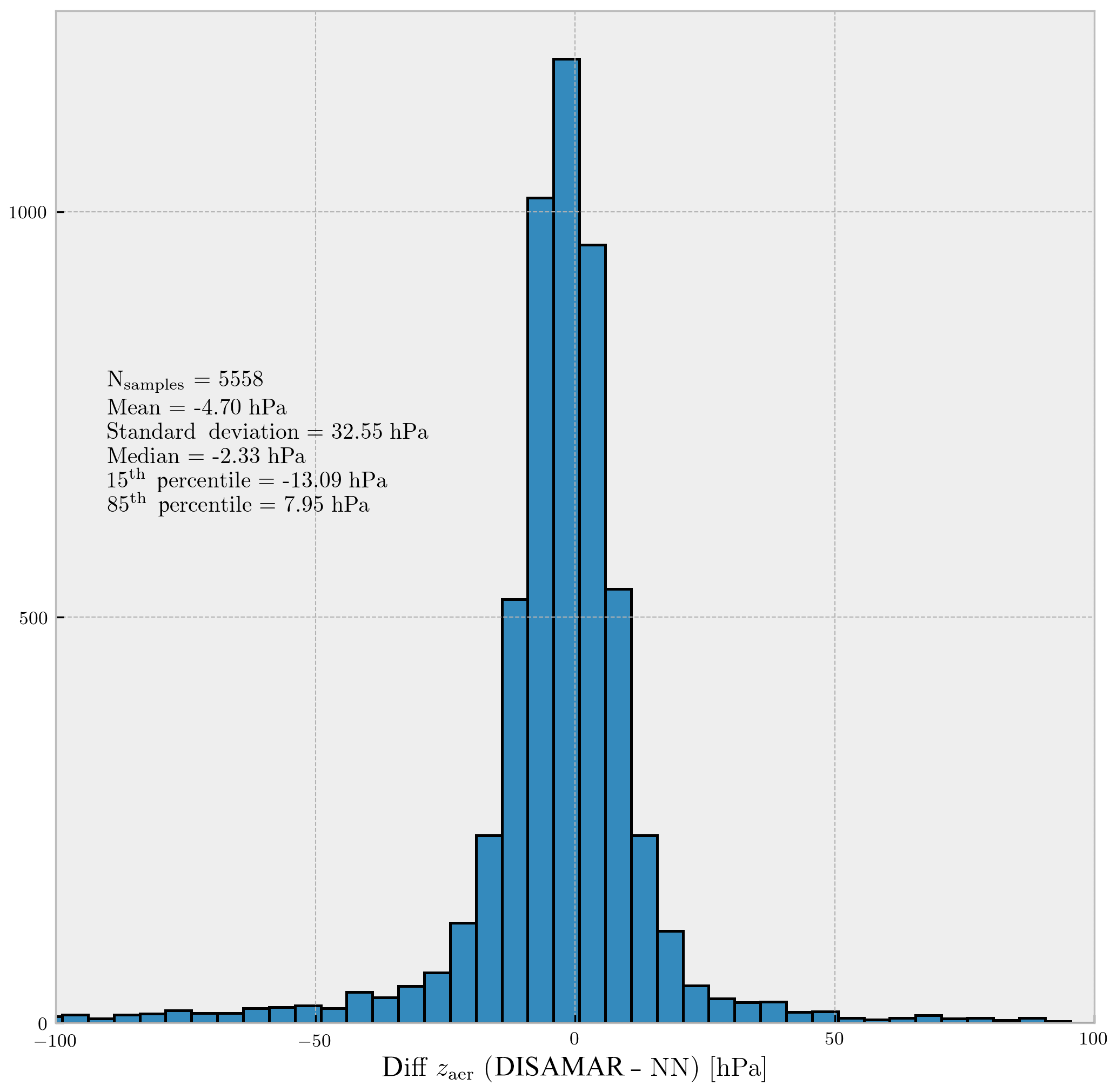
Figure 6 Histogram of differences between the retrieved z_aer values using DISAMAR and NN retrieval methods for synthetic spectra generated by DISAMAR. The total number of cases is 8000, whereas the plot contains 5558 retrieved samples for both DISAMAR and NN; non-converged cases are not included. A map of these differences is plotted in Fig. 9c.

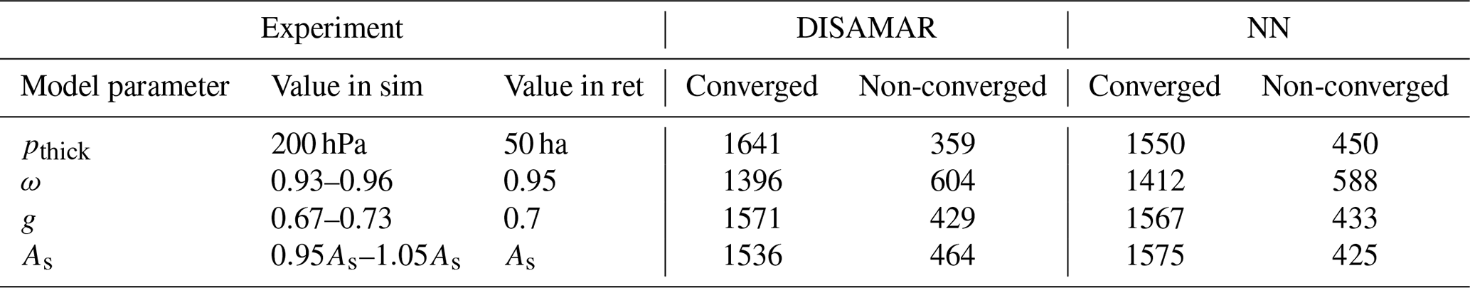
Table 3 A count of converged and non-converged results from synthetic experiments (sim) comparing retrieved (ret) aerosol layer heights between DISAMAR and NN.

The retrieved aerosol layer heights from DISAMAR and NN in the presence of model errors in aerosol layer thickness were found to be similar (Fig. 5a), with a Pearson correlation coefficient close to 1.0. Introducing model errors in other aerosol properties such as single scattering albedo (Fig. 5b) and scattering phase function (Fig. 5c) also resulted in a similar agreement between DISAMAR- and NN-retrieved aerosol layer heights. Furthermore, both methods also retrieved similar aerosol layer heights in the presence of model errors in surface albedo (Fig. 5d).

A total of 5558 retrievals from the 8000 different cases converged to a final solution. On average, z_aer retrieved using NN differed by approximately 5.0 hPa from z_aer retrieved using DISAMAR (Fig. 6), with a median of approximately 2.0 hPa. The spread of the retrieval differences was minimal, with the majority of the retrievals differing by less than 13.0 hPa. Differences close to and above 100.0 hPa did exist, but such retrievals were very uncommon.

From the 8000 scenes within the synthetic experiment, NN retrieved aerosol layer heights for 546 scenes where DISAMAR did not. Conversely, 586 scenes converged for DISAMAR and not for NN. A comparison of the biases from these odd retrieval results is plotted in Fig. 7, which indicates that retrievals from NN in cases where DISAMAR fails are realistic as the distribution of the biases is very similar to those cases when DISAMAR succeeds and NN does not (Fig. 7). Retrievals using the NN forward model required three more iterations on average to reach a solution compared with the retrievals by DISAMAR. Similarly, retrievals from DISAMAR had a significantly lower minimised cost function (4 orders of magnitude less on average) at the end of the retrieval compared with to NN. This is expected as NN cannot truly replicate DISAMAR. Having tested the NN-augmented retrieval algorithm in a synthetic environment, the retrieval algorithm was installed into the operational TROPOMI processor for testing with real data.

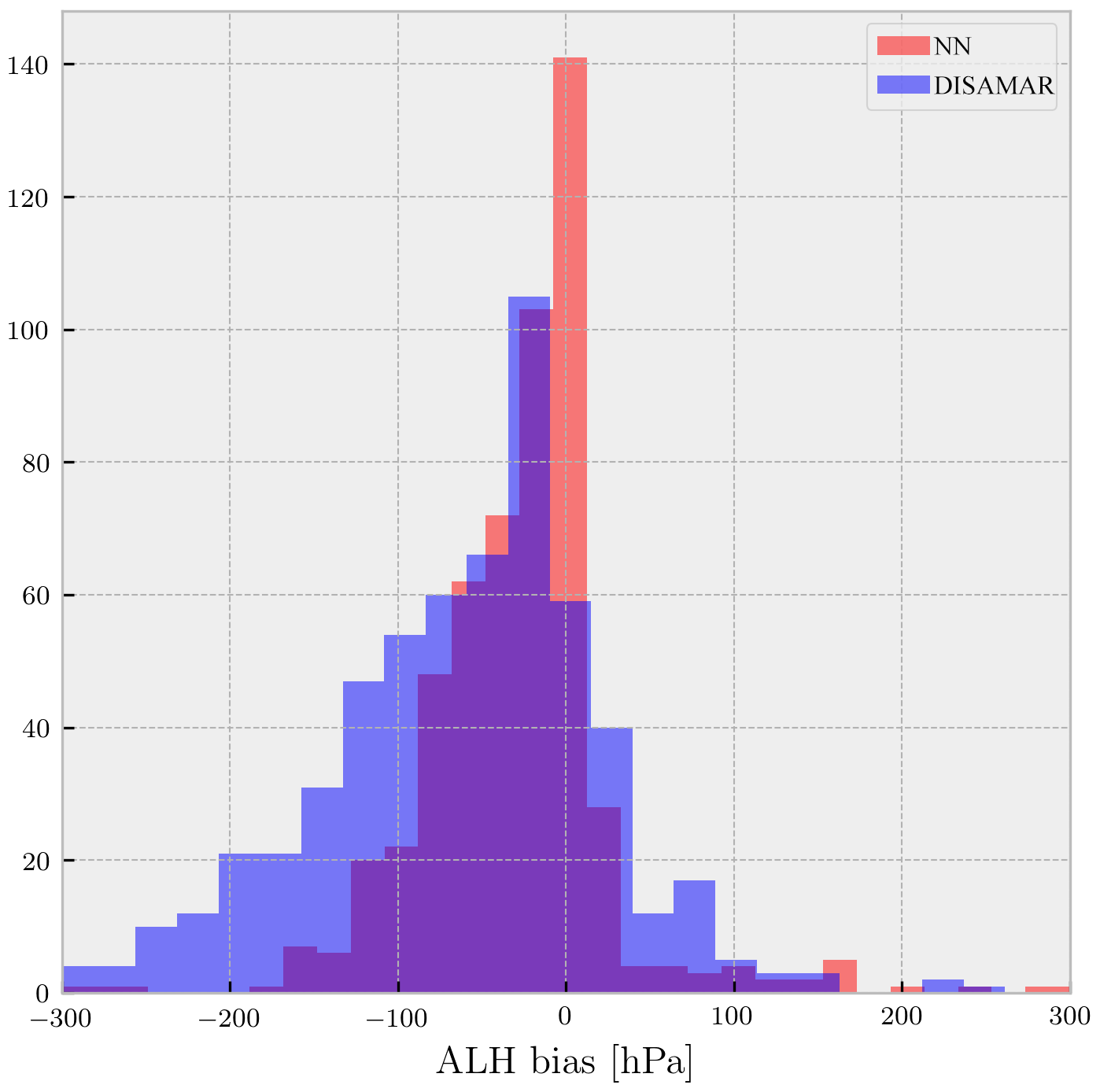
Figure 7 Histogram of biases (retrieved minus true) for scenes in the synthetic experiment for which either NN converges to a solution (red bar plot) and DISAMAR does not, or DISAMAR converges to a solution (blue bar plot) and NN does not.

4.2 Application to December 2017 Californian forest fires observed by TROPOMI

The December 2017 southern California wildfires have been attributed to very low humidity levels, following delayed autumn precipitation and severe multi-annual drought (Nauslar et al., 2018). Particularly on 12 December the region of the fires was cloud-free, owing to high-pressure conditions. A MODIS Terra image of the plume and the retrieved AAI from TROPOMI are shown in Fig. 8. The biomass burning plume extended well beyond the coastline and over the ocean (Fig. 8a), which provides a roughly cloud-free and low surface brightness test case for implementing the aerosol layer height retrieval algorithm. The AAI values were above 5.0 in the bulk of the plume (Fig. 8b), indicating a very high concentration of elevated absorbing aerosols. Pixels with an AAI value of less than 1.0 were excluded from the retrieval experiment. Cloud-contaminated pixels were removed from the data selected for processing using the FRESCO cloud mask product from TROPOMI (maximum cloud fraction of 0.2); parts of the biomass burning plume that did not contain any clouds were also removed as the cloud fraction values for these pixels were higher than the threshold. This is because FRESCO-based cloud fraction values over cloud-free scenes containing aerosols (biomass burning aerosols in this case) are generally expected to be positively biased. The retrieval algorithms did not process pixels on the coastline, where the surface albedo retrieval is likely to be wrong.

Figure 8 (a) MODIS Terra image of 12 December 2017 southern Californian wildfire plume, extending from land to ocean. (b) The calculated aerosol absorbing index from the TROPOMI Level-2 processor. Missing pixels are flagged by a cloud mask or land–sea mask, or have an AAI less than 1.0.

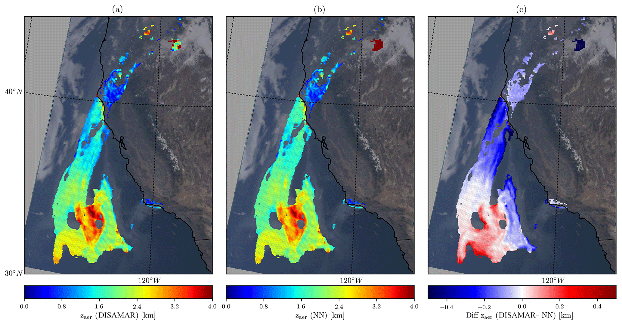
Figure 9 (a) Aerosol layer height retrieved using DISAMAR as the forward model. (b) The same, but with NN replacing DISAMAR in the operational processor. (c) Difference between DISAMAR and NN retrieved aerosol layer heights.

Figure 9 compares the retrieved z_aer over the plume using the line-by-line and neural-network-based forward models respectively. The number of converged retrievals is 7418 for the line-by-line algorithm, but 7370 for the neural network algorithm. The differences between z_aer (DISAMAR) and z_aer (NN) are up to 0.5 km (Fig. 9c). The majority of the negative differences are for the part of the plume extending from the coast between 47 and 40^∘ N. Figure 10 provides plots for further comparison between the two retrieval techniques. The neural-network-augmented processor retrieved aerosol layer heights which were (on average) less than 50.0 m from the retrieved aerosol layer heights by DISAMAR (Fig. 10b). The standard deviation of the differences is approximately 160 m, which indicates the presence of outliers. However, the majority of the differences in the two retrievals are less than 100 m; this is indicated by the 15th and the 85th percentile of these differences of −115.0 and 40.0 m respectively. Although the retrieval algorithms show good agreement, they primarily differed for the lower aerosol loading scenes (Table 4). The majority of the pixels where the neural network algorithm differed from the line-by-line counterpart by more than 200 m were for AAI values of less than 2.0 (Fig. 10c). Most of these biases were caused by an over-estimation of the retrieved aerosol layer height using the neural network algorithm, in comparison to the points from DISAMAR. Pixels with AAI values larger than 5.0 also showed a consistent bias of 60 m with a standard deviation of 30 m. This bias is not well understood.

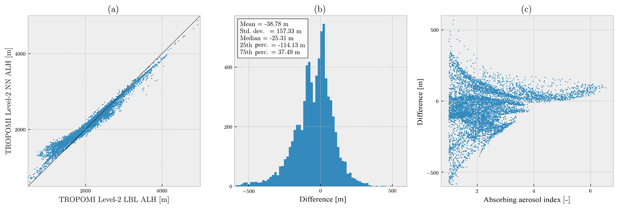
Figure 10 Comparison of retrieved aerosol layer heights from TROPOMI-measured spectra (orbit number 858) for the 12 December 2017 southern California fires using DISAMAR and NN. (a) Retrieved aerosol layer heights from the two methods. (b) Histogram of the difference between retrieved heights from DISAMAR and NN. The difference is defined as z_aer(DISAMAR)−z_aer(NN). (c) Differences compared with TROPOMI's operational AAI product (x axis).

Table 4 Statistics of difference between retrieved z_aer from DISAMAR and NN from Fig. 9c.

The time required by the line-by-line operational processor was 184.01±0.50 s per pixel, whereas the time required by the neural network processor was 0.167±0.0003 s per pixel. The neural network algorithm shows an improvement in the computational speed by 3 orders of magnitude over the line-by-line retrieval algorithm. The computational speed gained from implementing NN enables the retrieval of aerosol layer heights from all potential scenes in the entire orbit within the stipulated operational processing time slot.

5 Conclusions

Of the algorithms that currently retrieve TROPOMI's suite of Level-2 products, the aerosol layer height processor is an example of one that requires online radiative transfer calculations. These online calculations have traditionally been tackled with KNMI's radiative transfer code DISAMAR, which calculates (among other parameters) sun-normalised radiances in the oxygen A-band. There are, in total, 3980 line-by-line calculations per iteration in the optimal estimation scheme, requiring several minutes to retrieve aerosol layer height estimates from a single scene. This limits the yield of the aerosol layer height processor significantly.

The bottleneck is identified to be the number of calculations DISAMAR needs to carry out at every iteration of the Gauss–Newton scheme of the estimation process. As a replacement, this paper proposes using artificial neural networks in the forward model step. Three neural networks are trained for the sun-normalised radiance and the derivative of the reflectance with respect to aerosol layer height and aerosol optical thickness, which are the two state vector elements. As the goal is to replicate and replace DISAMAR, line-by-line forward model calculations from DISAMAR were used to train these neural networks. A total of 500 000 spectra were generated using DISAMAR, and each of the neural network models was trained for a total of 1 million iterations with the mean squared error between the training data output and the neural network output being the cost function to be minimised in the optimisation process.

Over a test data set with 100 000 different scenes unique from the training data set, the neural network models performed well, with errors generally not exceeding 1 %–3 % in the predicted spectra and derivatives. Having tested the neural network models for prediction errors in the forward model output spectra, they were implemented into the aerosol layer height breadboard algorithm and further tested for retrieval accuracy. In order to do so, experiments with synthetic as well as real data were conducted. The synthetic scenes included 2000 spectra with different model errors in aerosol and surface properties. In these cases, the neural network algorithm showed very good compatibility with the aerosol layer height algorithm, as it was able to replicate the biases satisfactorily.

We evaluate aerosol layer heights retrieved from TROPOMI measurements over southern California on 12 December 2017, when the fire plume extensively floats from land to ocean over a dry and almost cloudless scene. Operational retrievals using both DISAMAR and the neural network forward models showed very similar results, with a few outliers around 500 m for pixels containing low aerosol loads. These biases were outweighed by the upgrade in the computational speed of the retrieval algorithm, as the neural-network-augmented processor observed a speed-up of 3 orders of magnitude, making the aerosol layer height processor operationally feasible. Having achieved this improvement in its computational performance, the aerosol layer height algorithm is planned to operationally retrieve the product for all possible pixels in each orbit of TROPOMI. Such a boost in processor output allows for better analyses of retrievals and offers the possibility of removing some of the forward model simplifications mentioned in Sect. 2.2, which then paves the way to further develop the TROPOMI aerosol layer height algorithm.