On the zero-level offset in the GOSAT TANSO-FTS O₂ A band and the quality of solar-induced chlorophyll fluorescence (SIF): comparison of SIF between GOSAT and OCO-2

Satellite remote sensing of solar-induced chlorophyll fluorescence (SIF) has attracted attention as a method for improving the estimation accuracy of the photosynthetic production of terrestrial vegetation in recent years. The Greenhouse gases Observing Satellite (GOSAT) has the ability to observe both SIF and the concentrations of CO₂ and CH₄ and thus is expected to contribute to the understanding of the global carbon budget. Evaluating artefact signals (e.g. zero-level offset caused by non-linearity in the analogue circuit in the case of GOSAT) is effective for inferring the instrument status and important for retrieving SIF from satellite measurements. Here we investigate the characteristics of the zero-level offset and the consistency of satellite-derived SIFs by comparing the derived SIF with the Orbiting Carbon Observatory-2 (OCO-2) SIF at multiple spatial scales (footprint to global). The zero-level offset was evaluated using filling-in signals over bare soil while investigating the criteria for identifying barren areas. An analysis of the temporal variation of the zero-level offset over a period of 9 years suggests that the radiometric sensitivity of the GOSAT spectrometer changed after switching the optics path selector in January 2015. The GOSAT SIF was highly consistent with the OCO-2 SIF, with a bias within 0.1 mW m⁻² nm⁻¹ sr⁻¹ for most months and an inter-region bias of about 0.2 mW m⁻² nm⁻¹ sr⁻¹. Our results agree with the previous comparisons and support the consistency among the present satellite SIF data, which is important for the utilization of those data.

1 Introduction

Accurate estimation of the photosynthetic production of terrestrial vegetation is important to understand and predict the global carbon cycle and climate change. Global observation of solar-induced chlorophyll fluorescence (SIF) from satellite data has attracted attention as a potential means of reducing the uncertainties in the estimation of photosynthetic production (Stoll et al., 1999; Moya et al., 2004). SIF is a weak radiation emitted by chlorophylls during the photosynthesis process and thus is considered to be a better proxy for photosynthetic activity than the conventional vegetation indices. Frankenberg et al. (2011a) showed that the variation in fractional depth (filling in) of the Fraunhofer line by SIF can be detected by satellite sensors having a high spectral resolution at the wavelength domain without the telluric absorption lines in the O₂ A band. Since then, SIF retrievals have been performed by retrieving the signal that leads to filling in of the Fraunhofer line (filling-in signal) from the spectra of the Thermal And Near infrared Sensor for carbon Observation – Fourier Transform Spectrometer (TANSO-FTS) on board the Greenhouse gases Observing Satellite (GOSAT) (Joiner et al., 2011; Frankenberg et al., 2011b). GOSAT was launched on 23 January 2009 and has been operating for more than 10 years. The primary target of its measurement is the concentration of carbon dioxide and methane in the Earth's atmosphere.

Spectra of the TANSO-FTS O₂ A band include the zero-level offset, which is a spectrally constant additive signal caused by non-linearity in the analogue circuit and the analogue-to-digital converter (ADC) (Kuze et al., 2012). The intensity of the zero-level offset varies according to the radiance input to the TANSO-FTS (Kuze et al., 2012). Frankenberg et al. (2011b) retrieved the filling-in signal from the spectra of the TANSO-FTS over Antarctica (SIF = 0) and showed that the zero-level offset is on the same level as SIF and thus should be corrected to obtain SIF. The zero-level offset is also a non-negligible factor for the retrieval of column-averaged dry-air mole fractions of carbon dioxide (XCO₂) and methane (XCH₄) from the multiple bands of the TANSO-FTS as it affects the retrieval of aerosol parameters and surface pressure from the O₂ A band (Frankenberg et al., 2012). Moreover, the instrument status – e.g. the level of radiometric degradation – is reflected in the relationship between the zero-level offset and the observed radiance, which might have been affected by the pointing mechanism switch in January 2015 (Kuze et al., 2016). By using cloudy ocean data and bare soil data, different filling-in signals have been obtained between the Northern Hemisphere and the Southern Hemisphere and between different months (Joiner et al., 2012; Guanter et al., 2012). However, studies that focus on the characteristics of the zero-level offset have been limited to the initial period of the GOSAT observation. Furthermore, detailed evaluations have not been conducted on the criteria for identifying vegetation-free areas.

To date, retrievals of SIF have been performed for other satellite sensors such as the SCanning Imaging Absorption spectroMeter for Atmospheric CHartographY (SCIAMACHY) (Joiner et al., 2012; Köhler et al., 2015), the Global Ozone Monitoring Instrument 2 (GOME-2) (Joiner et al., 2013, 2016), the Orbiting Carbon Observatory-2 (OCO-2) spectrometer (Frankenberg et al., 2014; Sun et al., 2018), the Atmospheric Carbon dioxide Grating Spectroradiometer (ACGS) on board the Chinese Carbon Dioxide Observation Satellite Mission (TanSat) (Du et al., 2018), and the TROPOspheric Monitoring Instrument (TROPOMI) (Köhler et al., 2018a). Evaluating the quality of SIF data and the consistency among SIFs obtained by different sensors is important to fully utilize those data to elucidate the photosynthesis activity of the terrestrial vegetation. Although agreement among satellite-derived SIF data has already been partly confirmed (Joiner et al., 2012, 2013; Köhler et al., 2015, 2018b; Du et al., 2018), there were limitations in the simultaneity of these observations, the overlap of the footprints, and the global coverage. These limitations were significantly reduced in a recent comparison between TROPOMI SIF and OCO-2 SIF (Köhler et al., 2018a).

This study sought to evaluate the zero-level offset in the GOSAT TANSO-FTS O₂ A band from the initial period of the GOSAT observation until recently and to investigate the consistency between the GOSAT-derived SIF and the SIF derived from other satellite sensors. For the filling-in signal, the difference among spectra identified by various criteria for barren areas is examined, and based on the results, evaluations of temporal variation of the zero-level offset and offset correction are conducted (Sect. 3). By comparing the derived SIF with the OCO-2 SIF, the consistency of SIF is investigated (Sect. 4). OCO-2 is chosen for the comparisons because it is expected to have a small random error due to the large amount of data. Moreover, OCO-2 SIF has previously been compared with airborne data (Sun et al., 2017), GOME-2 (Köhler et al., 2018b), TanSat, (Du et al., 2018), and TROPOMI (Köhler et al., 2018a). Comparisons between GOSAT SIF and OCO-2 SIF are performed at multiple spatial scales (footprint to global) while considering the difference in observation patterns and the characteristics of vegetation.

2 Materials and data processing

2.1 GOSAT

GOSAT was launched on 23 January 2009 and is on a sun-synchronous orbit at 666 km altitude with a 3 d recurrence and a descending node around 13:00 local time. It is equipped with two instruments: a Fourier transform spectrometer (TANSO-FTS) and a Cloud and Aerosol Imager (TANSO-CAI). The TANSO-FTS has three bands in the short-wavelength infrared (SWIR) region (an O₂ A band, a weak CO₂ absorption band, and a strong CO₂ absorption band (bands 1, 2, and 3) centred at 0.76, 1.6, and 2.0 µm, respectively) and records two orthogonal polarization components (hereafter called P/S components). The spectral resolution (sampling interval) of bands 1, 2, and 3 are about 0.011 to 0.012 nm, 0.045 to 0.064 nm, and 0.069 to 0.090 nm, respectively. The full widths at half maximum (FWHMs) of the instrument line shape function (ILSF) of bands 1, 2, and 3 are about 0.02 nm, 0.06 nm, and 0.10 nm, respectively. For the signal processing of the TANSO-FTS, the amplifier gain level can be controlled at different levels: high (H) and medium (M), according to the brightness of the target. Gain M is used over bright surfaces such as the Sahara and central Australia. The instantaneous field of view (IFOV) of the TANSO-FTS is 15.8 mrad, which corresponds to a circular surface footprint of about 10.5 km in diameter at nadir. The TANSO-FTS has a pointing mechanism with mirror driving angles of ±35^∘ in the cross-track direction and ±20^∘ in the along-track direction. GOSAT data were used without discriminating the observation angle. The optics path selector was changed from the primary one to the secondary one on 26 January 2015 as the along-track pointing of the primary system worsened. The TANSO-CAI is a push-broom imager and has four narrow bands in the near-ultraviolet to near-infrared regions centred at 0.38, 0.674, 0.87, and 1.6 µm with spatial resolutions of 0.5, 0.5, 0.5, and 1.5 km, respectively, for nadir pixels.

The TANSO-FTS L1B product (radiance spectral data) version V201.202 was used in the present study. We corrected the sensitivity degradation of the TANSO-FTS using a radiometric degradation model that is based on the on-orbit solar calibration data (Yoshida et al., 2012). The retrieval window was 756.0 to 759.1 nm (the short-wavelength side of band 1), within which there are four strong Fraunhofer lines without telluric absorption lines, which is a strategy similar to that of Frankenberg et al. (2011a). In this wavelength domain, the sampling interval is about 0.011 nm, and the FWHM of the ILSF is about 0.02 nm. The retrieval window around 771 nm, where weak O₂ absorption lines are located, was not used in the present study, so that the retrieval was not influenced by O₂ absorption, and thus it was not necessary to exercise caution with respect to the differences in SIF among different windows. The filling-in signal was retrieved in a similar manner as in previous studies that fitted the modelled and the observed spectra using a simple forward model (Frankenberg et al., 2011a; Joiner et al., 2011). The retrieval algorithm is based on a non-linear maximum a posteriori estimation, just as for the TANSO-FTS L2 SWIR XCO₂ and XCH₄ retrievals (Yoshida et al., 2011, 2013, 2017). The state vector consisted of a spectrally constant filling-in signal, spectrally linear surface albedo, and wavenumber dispersion. A clear sky was assumed in the forward model. Retrieval was conducted separately for the P- and S-polarization spectra, although a scalar radiative transfer code was used as the forward model. Precision error in each retrieved filling-in signal was calculated by error propagation assuming only the instrumental random noise. When calculating the mean value, the standard error was also calculated by error propagation by assuming the independence of each error.

The TANSO-CAI L1B product (radiance data) and L2 product (cloud coverage data) were used to confirm the cloud condition. The cloud fraction within the TANSO-FTS IFOV was calculated based on the integrated clear confidence level stored in the TANSO-CAI L2 product. The integrated clear confidence level is represented by a real number between 0 to 1 and given for each pixel of the TANSO-CAI. Pixels with an integrated clear confidence level lower than 0.33 were classified as cloudy pixels. The fraction of the cloudy pixels within the TANSO-FTS IFOV was then calculated.

Data satisfying all the following criteria were used for the subsequent analysis: (1) several data-quality flags stored in the L1B product and spectrum quality check utilizing the out-of-band spectra (Yoshida et al., 2017) are set as OK, (2) the solar zenith angle (SZA) is < 70^∘, (3) the signal-to-noise ratio (SNR) of band 1 P or S polarization is ≥70, (4) the mean squared value of the residual spectrum is ≤2, (5) the land fraction of the TANSO-FTS footprint is 100 % or 0 %, and (6) the data are acquired with gain H. Concerning the cloud screening, different criteria were used for evaluating the filling-in signal (Sect. 3) and comparison with OCO-2 (Sect. 4).

2.2 OCO-2

OCO-2 was launched on 2 July 2014 and is on a sun-synchronous orbit with a 16 d recurrence and an ascending node around 13:30 local time. Its instruments consist of three grating spectrometers that measure spectra at the O₂ A band, the weak CO₂ absorption band, and the strong CO₂ absorption band with sampling intervals of 0.015, 0.031, and 0.04 nm, respectively, and FWHM of 0.04, 0.08, and 0.10 nm, respectively. Each grating spectrometer has eight adjacent footprints across the swath with each surface footprint of 1.29 km × 2.25 km at nadir. There are three observation modes: the nadir, glint, and target modes. The SIF lite product version B8100r was used in the present study. This product includes SIF retrieved separately from windows around 757 nm and around 771 nm. We used SIF from the former window, which is similar to the window for the SIF used by GOSAT. Only data with a cloud flag from the Oxygen-A Band Cloud Screening Algorithm set to clear sky were used. The nadir mode and glint mode were used separately, since the SIF has been reported to be dependent on the viewing angle (Guanter et al., 2012; Köhler et al., 2018b; Zhang et al., 2018; Sun et al., 2017).

The retrieval window of OCO-2 SIF at 757 nm is 758.1 to 759.2 nm, which is not identical to that used by GOSAT, because the edge of the short-wavelength side of the O₂ A band is different between GOSAT and OCO-2. Therefore, it is expected that the GOSAT SIF is higher than the OCO-2 SIF because of the spectral shape of SIF. This difference was neglected when comparing GOSAT SIF and OCO-2 SIF, since it was expected to be only 3 % to 4 % according to the observations at leaf level (Rascher et al., 2009; Magney et al., 2017) and simulations at the canopy level (Joiner et al., 2013; Verrelst et al., 2016). Although the Equator crossing time is not very different between GOSAT and OCO-2, the difference in observation time becomes large for high-latitude areas. The differences in the location and size of the footprint, observation time, and viewing angle between the two satellites were taken into account for the comparison. The detailed comparison method is described in Sect. 4.1.

2.3 NDVI, LAI, and land cover type

We used the normalized difference vegetation index (NDVI) to identify vegetation-free areas for the zero-level offset correction (Sect. 3) and the leaf area index (LAI) and land cover type to select SIF data of GOSAT and OCO-2 suitable for comparisons (Sect. 4). The Moderate Resolution Imaging Spectroradiometer (MODIS) products were used: NDVI monthly L3 global 1 km product (MYD13A3; Didan, 2015), LAI 4 d L4 global 500 m product (MCD15A3H; Myneni et al., 2015), and land cover type yearly L3 Global 500 m product (MCD12Q1; Friedl and Sulla-Menashe, 2015). The land cover type derived by the International Geosphere-Biosphere Programme (IGBP) classification scheme was used. These data were transformed to a geographic grid of 0.02^∘ latitude by 0.02^∘ longitude by nearest-neighbour resampling. For LAI, the dataset for each 4 d interval was adopted to calculate the monthly mean value if the 4 d were included in the month. NDVI and LAI within the TANSO-FTS footprint was obtained by calculating the mean values of 5 pixels × 5 pixels, with the centre pixel including the centre of the TANSO-FTS footprint. The land cover type of the TANSO-FTS footprint was also defined using 5 pixels × 5 pixels, but the detailed treatment differed between comparison methods (Sect. 4.1). For OCO-2, the LAI and land cover type were obtained from the single-pixel value of each MODIS product, including the centre of the OCO-2 footprint.

3 GOSAT filling-in signal and zero-level offset correction

3.1 Current state of evaluation of the zero-level offset

The retrieved filling-in signal from the GOSAT spectra consists of SIF and the zero-level offset, and thus correction for the zero-level offset is required to derive SIF (SIF is equal to the filling-in signal minus the zero-level offset, Frankenberg et al., 2011b). The zero-level offset can be represented by the filling-in signal over vegetation-free areas (SIF = 0). Initially, the filling-in signal over Antarctica was used to evaluate the zero-level offset (Frankenberg et al., 2011b). The results of this analysis showed a strong correlation between the zero-level offset and the averaged radiance of the TANSO-FTS band 1. However, the spatio-temporal coverage of the Antarctica data was limited. A cloudy ocean area (Joiner et al., 2012) and bare soil area (Guanter et al., 2012) were subsequently used. Together, these two studies reported the characteristics of the zero-level offset, i.e. the difference between the Northern Hemisphere and the Southern Hemisphere and the temporal variation (from the boreal summer of 2009 to the boreal spring of 2011). The TANSO-FTS L1B products version V050.050 to V110.110 were used in the above-mentioned studies. The newer version (V201.202) was used in the present study. Although the band 1 non-linearity correction in the TANSO-FTS L1B product has been updated (Kuze et al., 2012, 2016), the filling-in signal retrieved in the present study (Sect. 2.1) shows dependence of the zero-level offset on the observed radiance (Fig. S1 in the Supplement), indicating that the zero-level offset correction is still required. By considering the above-mentioned studies, the filling-in signal over bare soil was investigated over a long period of time in the present study, since such areas seem to be suitable for the zero-level offset correction for terrestrial vegetation.

3.2 Filling-in signal over bare soil

To identify spectra over bare soil, Guanter et al. (2012) used criteria of R₁<R₂ or R₂<R₃, where R_i is the top-of-the-atmosphere (TOA) reflectance of the TANSO-FTS SWIR band i. We investigated the effectiveness of these criteria by using the filling-in signal over areas having different NDVI values. In the present study, the retrieved albedo values were used (hereafter R_i denotes the retrieved albedo value of band i). Only data with the TANSO-CAI cloud fraction of 0 were used in this section since the filling-in signal might vary according to the cloud fraction. Monthly variation of the filling-in signal was calculated using data identified by different criteria (R_i values or NDVI values) (Fig. S2). The variation of the filling-in signal according to the criteria of albedo values and NDVI values was similar between P and S polarization. The filling-in signal clearly increased with the increase in NDVI, showing the influence of SIF from terrestrial vegetation on the filling in.

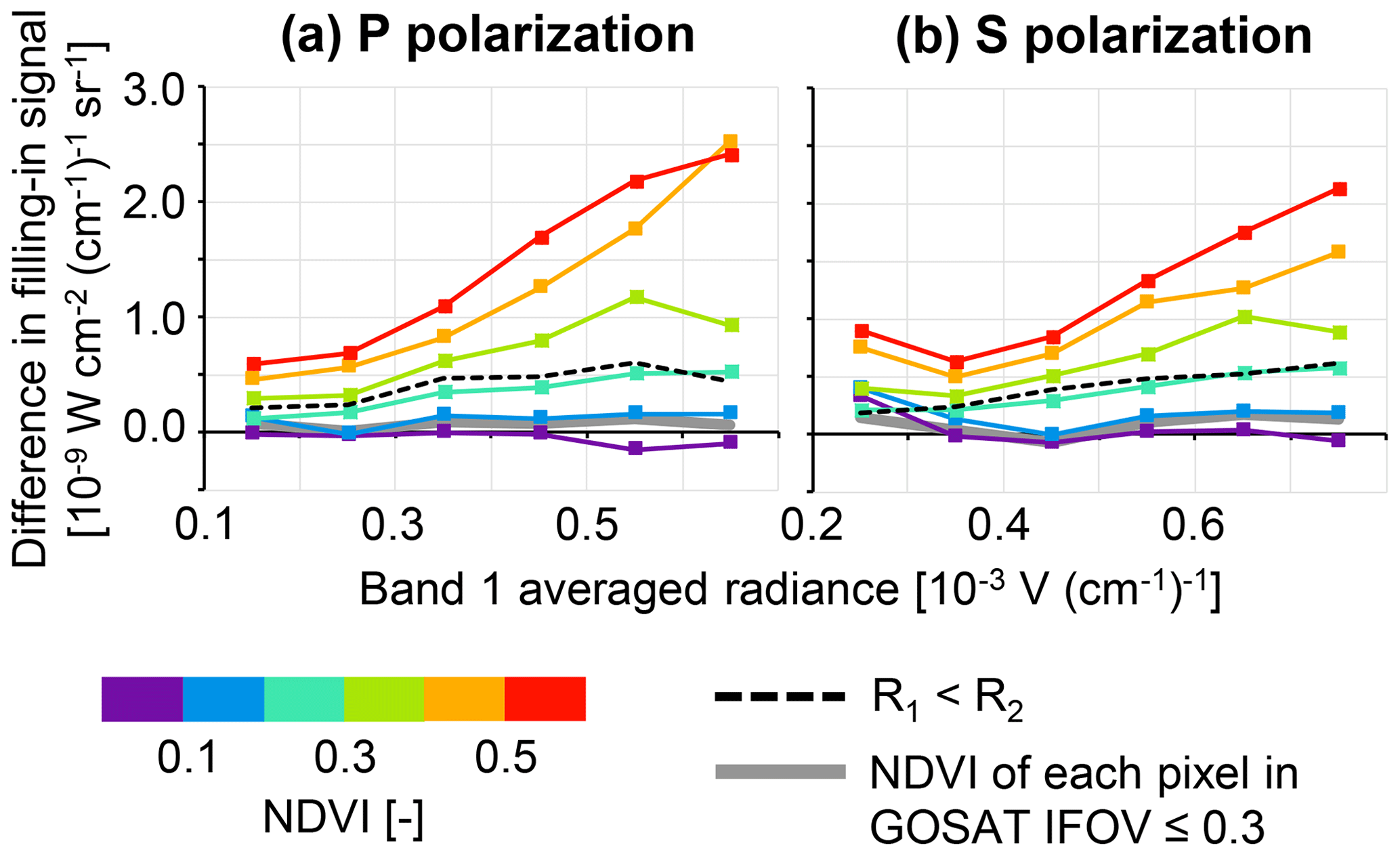
Figure 1 Temporal mean (May 2009 to January 2018) of the difference in the monthly mean filling-in signal between data with R₂<R₃ (R_i: albedo for the TANSO-FTS band i) and data having different NDVI values, plotted against the averaged radiance of the TANSO-FTS band 1 for 30 to 45^∘ N: (a) P polarization; (b) S polarization. Results derived from the data with R₁<R₂ (dotted black line) and data with NDVI_max≤0.3 (solid black line) are also plotted.

The difference in the filling-in signal was calculated for each month between data identified by the criteria of R₂<R₃ and those identified by other criteria (NDVI values and R₂<R₃), and the difference was averaged over a target time period (May 2009 to January 2018) (Fig. 1). The calculation was conducted for each level of averaged radiance of the TANSO-FTS band 1 (horizontal axis of Fig. 1). The global distribution of the averaged radiance is shown in Fig. S3, and the averaged radiance for vegetated areas is shown in Fig. S4. The difference shown in Fig. 1 for R₁<R₂ was higher than that for low NDVI values. It seems that SIF was included in the filling-in signal for R₁<R₂. These criteria identify a large number of data (Fig. 2a) but are considered to identify vegetated areas. Concerning Fig. 2, it should be noted that, unlike OCO-2, GOSAT data over the Sahara cannot be used to evaluate the zero-level offset because of the different gain setting, which increases noise in the evaluated zero-level offset. The difference in filling-in signal between data with R₂<R₃ and those with NDVI ≤0.2 was almost 0, irrespective of the observed TANSO-FTS radiance and polarization. According to Fig. 2b, the data identified by criteria R₂<R₃ were limited to specific areas that appeared to be barren. These results indicate that the criteria of R₂<R₃ offer a small number of data but are robust for the identification of vegetation-free areas. The criteria of NDVI ≤0.2 offered a larger number of data and wider spatial coverage compared to the criteria of R₂<R₃ (Fig. 2b, c). The difference shown in Fig. 1 became larger for NDVI > 0.2, especially in the case of a high radiance level. For NDVI 0.2 to 0.3, the difference was comparable to that for the criteria of R₁<R₂ (black dotted line in Fig. 1). For these cases, the difference was within 0.1 in SIF units (mW m⁻² nm⁻¹ sr⁻¹). It should be noted that the difference shown in Fig. 1 is the time mean value, and this difference became large in summer (Fig. S2). Moreover, another set of criteria using NDVI were tested: NDVI_max≤0.3 for 5 pixels × 5 pixels around the centre of the TANSO-FTS footprint. The filling-in signal for these criteria showed a similar tendency to that for mean NDVI ≤ 0.2 (grey solid line in Fig. 1), and these criteria offered a larger number of data (Fig. 2d). We suggest a new set of criteria: R₂<R₃ or mean NDVI ≤ 0.2 or NDVI_max≤0.3. We accepted data with a cloud fraction ≤ 0.2 because the results hardly varied within this cloud fraction (Figs. S5 and S6).

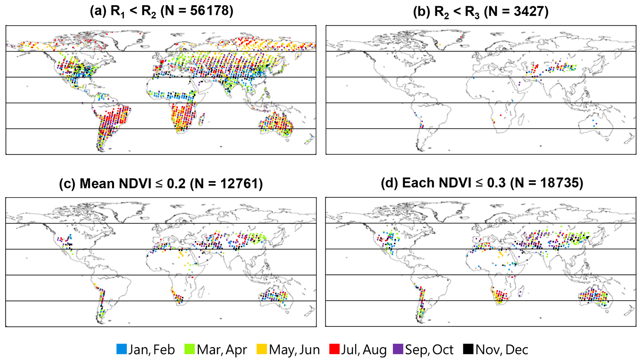
Figure 2 Locations of data identified as the candidates for vegetation-free areas by the albedo values (R_i for TANSO-FTS band i) or NDVI values for P polarization in 2016: (a) R₁<R₂; (b) R₂<R₃; (c) mean NDVI ≤ 0.2; (d) NDVI_max≤0.3. The numbers of data points (N) are also presented.

3.3 Temporal variation of zero-level offset

Figure 3 shows the temporal variation of the zero-level offset evaluated from bare soil (criteria shown in Sect. 3.2). The ranges of the observed radiance used in Fig. 3 correspond to the high and low side of the observed radiance for vegetated areas (Figs. S3 and S4). The zero-level offset for P polarization showed a sharp decrease after GOSAT started its observations. In contrast, the variation in S polarization was small. The decrease in P polarization became gentle at around early 2011. For both polarizations, the gradient of the temporal variation of the zero-level offset changed in February 2015 following the switch from the primary to the secondary TANSO-FTS optics path selector on 26 January 2015. The zero-level offset evaluated from a cloudy ocean area shows a similar temporal pattern (Figs. S7 and S8).

Figure 3 Temporal variation of the zero-level offset evaluated from bare soil within the latitude zone of 30 to 45^∘ N: (a) P polarization; (b) S polarization. Results for different ranges of the observed radiance are depicted in each panel. The bare soil data were identified by the criteria determined in Sect. 3.2.

A possible cause of such a temporal variation is a variation in the instrumental characteristics related to the zero-level offset itself (analogue circuit and ADC) and to the radiance (radiometric degradation of the TANSO-FTS). The degradation does not directly change the fractional depth of the Fraunhofer line; however, a discrepancy between the actual radiance input to the TANSO-FTS and the observed radiance affects the relationship between the zero-level offset value and the observed radiance. The initial decrease in P polarization appears to mainly relate to the variation in characteristics of the analogue circuit and the ADC. This is supported by the fact that the radiometric degradation model was generated using the on-orbit solar calibration data covering the time period when the zero-level offset was decreasing (Yoshida et al., 2012). In addition, the initial decrease was observed only for P polarization, although the degradation correction was conducted in the same way for both polarizations. Of course, there is a possibility that the discrepancy between the degradation model and the actual degradation is not minimal, since it is difficult to accurately model the rapid radiometric degradation using the monthly on-orbit calibration data (Yoshida et al., 2012). There is also a possibility that the accuracy of the degradation model differs between P and S polarization. On the other hand, the decrease in the zero-level offset from February 2015 for both polarizations seems to have been caused by radiometric degradation of the TANSO-FTS. The degradation correction factors are predicted values after about 3 years from the launch of GOSAT under the assumption that the degradation becomes slower with time in general. It is necessary to re-evaluate the degradation after the optics path selector is changed.

Frankenberg et al. (2011b) used only S-polarization data because the zero-level offset for P polarization showed significant time dependence. On the other hand, Guanter et al. (2012) reported a decrease in the zero-level offset for both P and S polarization. Our results agree with those of Frankenberg et al. (2011b). Guanter et al. (2012) indicated that the temporal variation of the zero-level offset corresponded to that of the spectral slope. Although our analysis showed no clear relationship between the zero-level offset and the spectral slope (Fig. S9), the difference in the slope of the spectral slope before and after February 2015 supports the idea that the characteristics of the instrument changed after the TANSO-FTS optics path selector was switched from the primary one to the secondary one.

In addition to the aforementioned general variations, periodic variations, in which small offset values were seen during winter (Fig. 3), and differences between the Northern Hemisphere and the Southern Hemisphere (Fig. S10) were also observed. The periodic variation (Guanter et al., 2012) and difference between the hemispheres (Joiner et al., 2012) were reported in previous studies. As discussed in those studies, the cause of such a variation in the zero-level offset seems to be the instrumental effects that vary with orbit phase and season (e.g. the detector temperature and condition of analogue circuits) and rotational Raman scattering (RRS). We investigated the variation of the zero-level offset against the detector temperature and found no clear relationship (Figs. S11 and S12). A large sampling step of the recorded temperature (∼0.08 K) might obscure the relationship. The aforementioned periodic and latitudinal variation correspond to the increase in the zero-level offset according to the decrease in SZA, which is the opposite of the tendency for the expected filling in by RRS. Moreover, assumptions regarding the retrieval, solar irradiance model, and unpolarized forward model could affect the retrieved filling in and albedo, respectively, but do not seem to account for the spatio-temporal variation of zero-level offset.

3.4 Calculating SIF by correcting the zero-level offset

For each TANSO-FTS spectra, SIF was calculated separately for P and S polarization by subtracting the zero-level offset from the filling-in signal. The zero-level offset was determined using a table representing the variation of the zero-level offset according to time and the averaged radiance of the TANSO-FTS band 1. The table was generated using the zero-level offset evaluated from bare soil over the globe by binning the zero-level offset against the averaged radiance with an interval of 0.00003 V (cm${}^{-\mathrm{1}}{)}^{-\mathrm{1}}$ for each month. Data from the Northern Hemisphere and the Southern Hemisphere were used with no separation to increase the number of data and the coverage of the TANSO-FTS radiance. The table was generated separately for P and S polarization, and the mean value and standard error were calculated for each bin. The bin size of the TANSO-FTS radiance was determined so that the variation of the zero-level offset is well represented and the number of data for each bin are ensured. The difference between the zero-level offset binned with 0.00003 V (cm${}^{-\mathrm{1}}{)}^{-\mathrm{1}}$ and that binned with a finer interval was small (Fig. S13). It is assumed that the difference becomes minimal when SIF values having different TANSO-FTS radiances are averaged during the practical use of the SIF data. The standard error of the zero-level offset table for the TANSO-FTS radiance of vegetated areas (Fig. S4) was about 0.03 to 0.1 mW m⁻² nm⁻¹ sr⁻¹ (Fig. S14). SIF calculation was conducted unless the offset value of the bin was derived from less than 10 data points. Subsequently, the SIF derived from P and S polarization was averaged under the assumption that the difference in SIF between the polarizations is minimal.

4 Comparison between GOSAT SIF and OCO-2 SIF

4.1 Comparison method

The SIF values derived from satellite observation vary according to the observation time, viewing direction, observed wavelength, and type and condition of vegetation. When comparing SIF data among satellite sensors, it is necessary to account for each of these factors. Joiner et al. (2012) compared the global distribution and seasonal cycle for specific regions between GOSAT SIF and SCIAMACHY SIF while considering the difference in wavelength. In a subsequent study, the same authors (Joiner et al., 2013) compared the global distribution of SIF derived from GOME-2 with that from GOSAT. Recently, more refined comparisons have been performed. Although their analysis was limited to the Amazon region, Köhler et al. (2018b) compared OCO-2 SIF and GOME-2 SIF using data with a footprint covering the target land cover type (evergreen broadleaf) and considering the difference in observation geometry (the angle of incident sunlight and observation). Köhler et al. (2018a) also compared TROPOMI SIF with OCO-2 SIF using matching criteria in which the OCO-2 footprint was included in the TROPOMI footprint and the difference in overpass time and observation geometry was small (10 min and 20^∘ in phase angle, the angle between the observation direction and the incident sunlight, respectively). Normalization of SIF is effective to account for the difference in observation time between satellites. A simple approach is to divide SIF by cos(SZA) (as in Joiner et al., 2011). Frankenberg et al. (2011b) proposed an approximation formula to obtain the daily average SIF from the observed instantaneous SIF and the variation in SZA throughout a day. Both normalizations were based on the same principle to account for the variation in incident photosynthetically active radiation (PAR) under the assumption of a clear sky. Dividing by cos(SZA) apparently amplified the noise for SIF acquired under large SZA. The daily average SIF seems to be suitable when comparing with gross primary productivity (GPP).

Based on the aforementioned studies, we conducted three different comparisons between GOSAT and OCO-2: in Case 1 used a footprint level with strict matching criteria, Case 2 used a specific region with similar observation time, and Case 3 had a global scale (Sect. 4.2, 4.3, and 4.4, respectively). In Case 1 a simple comparison was performed using overlapped data. The matching criteria were that the OCO-2 footprint was included in the GOSAT footprint (the distance was less than 5 km between the footprint centre of the satellites) and the difference in observation time was within 15 min. OCO-2 SIFs satisfying these matching criteria were identified and averaged. To minimize the error due to the heterogeneity of the land cover, the land cover types within the satellite footprints were checked. If the majority of the land cover types were the same and the composition ratio of the land cover types was similar between GOSAT and OCO-2, the SIFs were used for comparison. The majority and composition ratio were defined against 5 pixels × 5 pixels (MODIS pixels) for GOSAT and the identified footprints for OCO-2. The criterion for the composition ratio was that the difference in the fraction of land cover type between GOSAT and OCO-2 was less than 0.2 for each IGBP type. The OCO-2 SIF derived from the nadir mode was used to minimize the influence of the difference in observation geometry. It is difficult to investigate the influence of observation geometry on SIF by comparing GOSAT SIF, OCO-2 nadir SIF, and glint SIF, because the number of data are expected to be small for the strict criteria of Case 1.

The land cover type and the number of data are limited in Case 1 because the GOSAT path and OCO-2 path cross within a specific latitude zone (around 30^∘ N). Case 2 made comparisons for specific regions having different vegetation coverage where the difference in the observation time was small. The target regions and land cover types were evergreen broadleaf forest in Southeast Asia, cropland in the Corn Belt region of the USA, and grassland in the southern part of the USA. GOSAT SIF data included in the target region and having a fraction of the target land cover type of ≥0.8 within the footprint were identified and averaged for each month. OCO-2 SIF data included in the target region and having the target land cover type were identified and averaged for each month. OCO-2 SIFs derived from the nadir mode and the glint mode were averaged separately. The mean LAI and the mean local time of the observation were calculated in the same way as SIF.

Case 3 made comparisons over the globe to confirm that the spatial variation of the zero-level offset was effectively corrected. The monthly mean SIF was calculated for each land cover type within a grid box of 5^∘ latitude by 10^∘ longitude. Concerning GOSAT, only SIF data for which the fraction of the land cover type was ≥0.8 within the footprint were used. For each grid, the land cover type containing the maximum number of GOSAT data was defined as the representative land cover type. SIF of the representative land cover type was compared between GOSAT and OCO-2. The mean LAI and the mean local time of the observation were calculated in the same way as SIF. If the difference in LAI between GOSAT and OCO-2 exceeded 20 %, the grid was not used for comparison. For this comparison, OCO-2 SIF derived from the nadir mode was used.

For each comparison, the phase angle was calculated to confirm the effect of observation geometry, as in Köhler et al. (2018b). Normalization that divides SIF by cos(SZA) was applied. We conducted a simple normalization, because the present study sought only to evaluate the difference in instantaneous SIF between satellite data. Only GOSAT data with a cloud fraction ≤ 0.2 were used. Comparisons were conducted for February 2015 to January 2018 because the GOSAT optics path selector was changed from the primary one to the secondary one in January 2015, and OCO-2 data were available from September 2014.

4.2 Case 1: comparison at the footprint level

Figure 4 shows a scatter plot of GOSAT SIF and OCO-2 SIF. The precision error of the single GOSAT SIF was 0.5 to 0.7 mW m⁻² nm⁻¹ sr⁻¹, making the plot of individual data dispersive; however, deviation of the plot according to the land cover type was not found. The standard error of OCO-2 SIF differed among the data according to the number of footprints used. The mean difference between GOSAT SIF and OCO-2 SIF was small (−0.05 mW m⁻² nm⁻¹ sr⁻¹). For binned data, the correlation was high, although GOSAT SIF was lower than OCO-2 SIF for areas having certain levels of OCO-2 SIF value.

Figure 4 Scatter plot of GOSAT SIF and OCO-2 SIF, whose footprints were included in the GOSAT TANSO-FTS footprint. Individual GOSAT data are depicted by small circles with colours representing the land cover type. OCO-2 SIF values between −0.1 and 2.1 mW m⁻² nm⁻¹ sr⁻¹ were binned with an interval of 0.2 mW m⁻² nm⁻¹ sr⁻¹, and the mean and standard error of GOSAT SIF and OCO-2 SIF were calculated for each bin.

When GOSAT SIF data having the absolute value of the matched OCO-2 SIF ≤ 0.1 mW m⁻² nm⁻¹ sr⁻¹ were identified and averaged, the standard error was 0.077 mW m⁻² nm⁻¹ sr⁻¹ (the number of data points was 68). The standard error used in the present study is the estimated value from the instrumental random noise. The standard error calculated using the actual variation (standard deviation of the identified GOSAT SIF divided by the square root of the number of data) was 0.097 mW m⁻² nm⁻¹ sr⁻¹. The actual variation was slightly larger than the estimated value, since the estimation was based on only instrumental random noise. However, the estimated standard error appeared to explain the primary variation.

Köhler et al. (2018b) calculated variations in SIF according to the phase angle using a three-dimensional radiative transfer model in the Amazon. Their results showed that SIF decreased significantly when the phase angle changed from 0^∘ (hot spot) to around 20^∘, and then it gently decreased when the phase angle became larger. Therefore, the effect of observation geometry on the results of this section seems to be small, because the phase angle was larger than 20^∘ for most cases and the difference in the phase angle between GOSAT and OCO-2 was about 10^∘ (Fig. S15a). Moreover, most of the SIF data used in this section appeared to be derived from land cover types with a simple structure (Fig. 4), and hence the effect of observation geometry was negligible, as shown in a later section comparing the OCO-2 nadir and glint SIF.

The above results confirm that GOSAT SIF and OCO-2 SIF agree on the zero level when overlapped footprints with similar observation times are used. This conclusion was hardly changed by changing the matching criteria between the GOSAT data and OCO-2 data (the land cover, topography, observation angle, and so on). The latitude zone was limited to 30 to 40^∘ N and the land cover mainly consisted of barren areas in this section. It was difficult to investigate the temporal variation of the difference between GOSAT SIF and OCO-2 SIF because of the strict matching criteria. The next section considers comparisons made using vegetated areas where the difference in observation time was small to investigate whether the agreement between GOSAT SIF and OCO-2 SIF is observed under high SIF emission.

4.3 Case 2: comparison for specific regions with similar observation times

Figure 5 shows the monthly variation of GOSAT SIF and OCO-2 SIF for three different vegetated areas. Panel (a) shows the variation for the evergreen broadleaf forest in Southeast Asia. In this region, the observation time of GOSAT was slightly earlier than that of OCO-2, but the difference was small (about 15 to 25 min). Although the difference in LAI was small between OCO-2 nadir and glint, the nadir SIF was higher than the glint SIF, especially in summer, revealing the effect of observation geometry (more shaded leaves were seen from glint observation than from nadir observation). Although fluctuations were found in GOSAT SIF, both GOSAT SIF and OCO-2 SIF showed a clear seasonal cycle, and the GOSAT SIF value was on a similar level to the OCO-2 nadir. When comparing the GOSAT and OCO-2 nadir SIFs, the effect of observation geometry seems to have been small, considering the phase angle. LAI was slightly higher for GOSAT than for OCO-2; however, the influence of this difference in LAI on SIF appeared to be small for such a high LAI condition (Koffi et al., 2015; Verrelst et al., 2016; Liu et al., 2017). The difference between the GOSAT SIF and OCO-2 nadir SIF did not correspond to the difference in LAI. However, the GOSAT SIF was higher than the OCO-2 nadir SIF for June. This finding appeared to be attributable to errors in the zero-level offset correction or random error, since the effects of other factors seemed to be small, as discussed above.

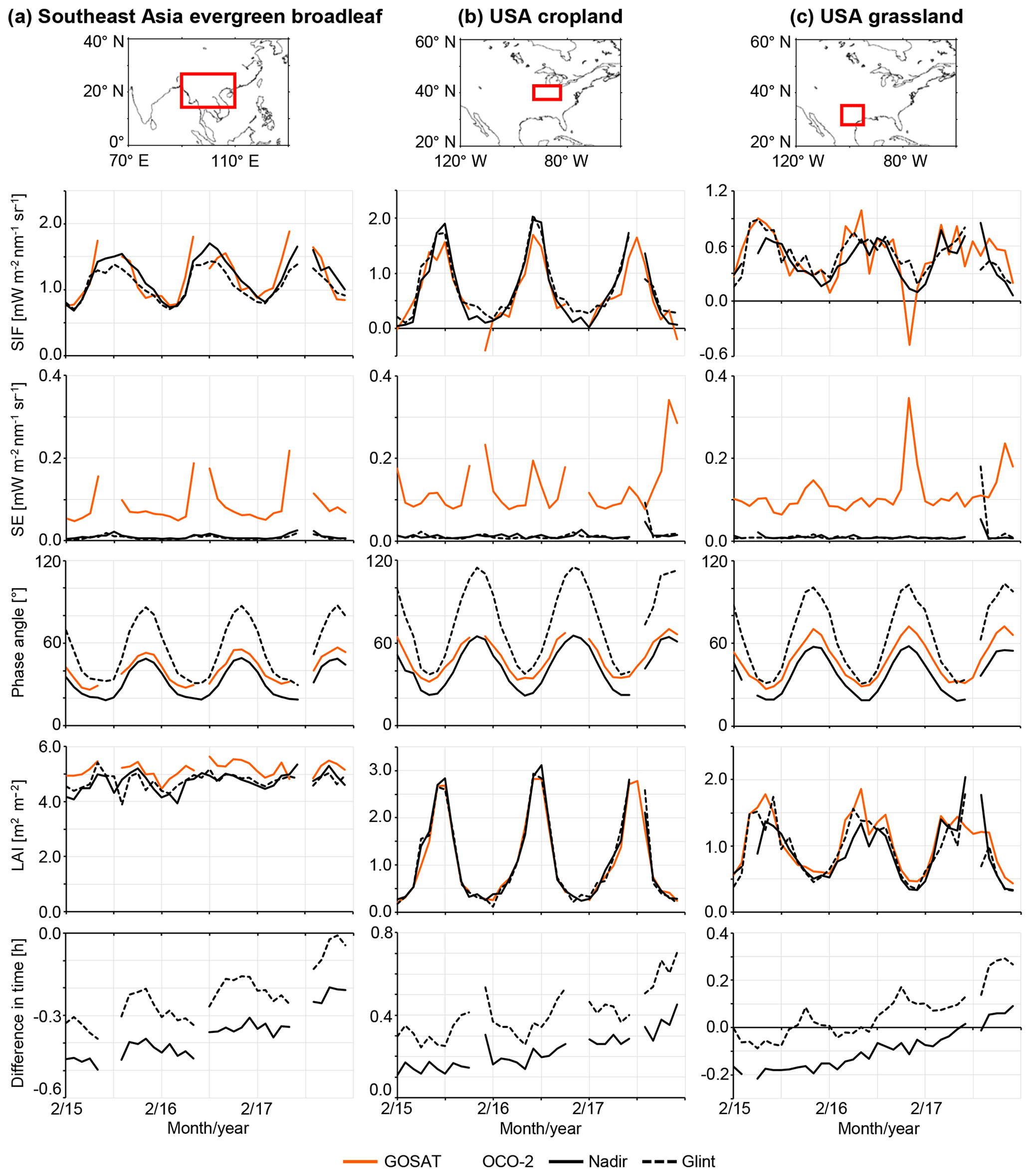
Figure 5 Comparison of the monthly mean SIF between GOSAT and OCO-2 for specific regions where the difference in the observation time is small: (a) evergreen broadleaf forest in Southeast Asia; (b) cropland in the USA; (c) grassland in the USA. In each panel, the target region, SIF value, standard error (SE), phase angle (angle between observation direction and incident sunlight), LAI, and difference in local time of the observation (GOSAT – OCO-2) are presented. Only months with more than four data points are plotted.

The results for cropland in the USA are shown in Fig. 5b. In this region, the observation time of GOSAT was slightly later than that of OCO-2, but the difference was slight. The difference in LAI and that in SIF between OCO-2 nadir and glint were also slight, indicating that the effect of observation geometry was small. In addition, the phase angle was larger than 20^∘, and thus the effect of observation geometry was minimal when comparing GOSAT and OCO-2 in this region. Although the GOSAT SIF showed a lower peak value in summer than OCO-2 SIF, the seasonal cycle of GOSAT SIF corresponded to that of OCO-2 SIF. The variation of GOSAT SIF of the cropland was smoother compared to that of the evergreen broadleaf forest in Southeast Asia, although the standard errors were comparable.

Figure 5c shows the comparison for grassland in the USA. The observation time was almost the same between GOSAT and OCO-2 in this region. OCO-2 glint SIF was higher than the nadir SIF for 2015 and 2016. This difference seems to correspond to the difference in LAI (e.g. there was a clear correspondence in May 2015 and the spring of 2016). The effect of observation geometry was expected to be minimal for the grassland, as discussed for the USA cropland. GOSAT SIF agreed with OCO-2 glint SIF both with respect to the seasonal cycle and the absolute value. The slightly higher SIF for GOSAT seemed to be explained by the difference in LAI. The correspondence between the variation in LAI and that in SIF supports the consistency among the GOSAT SIF, OCO-2 nadir SIF, and glint SIF. Concerning the finding that the GOSAT SIF value was lower than 0 in December 2016, this was probably attributable to the random error being dominant due to the small number of data for this region in this month (not offset table).

In this subsection, on the whole, GOSAT SIF agreed with OCO-2 SIF not only with respect to the seasonal cycle but also in terms of the absolute value for regions with high SIF emission. A large difference between GOSAT SIF and OCO-2 SIF was observed over several months, even when the number of GOSAT data were comparable with other months. In the next section we perform a comparison on a global scale to address these issues and to investigate whether the offset correction worked well in different locations around the world.

4.4 Case 3: comparison at a global scale

Figure 6 shows the difference in the monthly mean SIF and that in the monthly mean observation time between GOSAT and OCO-2 within a 5^∘ × 10^∘ grid box for July and December 2015. The difference in SIF was small for the latitude zone where the observation time was similar between the satellites. The observation time of GOSAT was later than that of OCO-2 in the northern high-latitude region and earlier than that of OCO-2 in the Southern Hemisphere. For the northern high-latitude region in July, GOSAT SIF was lower than OCO-2 SIF. This may indicate that the different observation times between GOSAT and OCO-2 captured the diurnal cycle of the SIF yield from terrestrial vegetation. Generally, SIF varies mainly according to the absorbed PAR (APAR); however, this pattern changes under any environmental stress. One typical example is plants under water stress: increase in fluorescence emission stops in the early morning at a specific level of APAR, and then the emission decreases toward the late afternoon independent of APAR owing to a decrease in SIF yield (Cerovic et al., 1996; Ounis et al., 2001; Flexas et al., 2002; Evain et al., 2004). In the present study, the difference in incoming PAR was accounted for by dividing SIF by cos(SZA). FAPAR (= APAR/PAR) was expected to be almost stable or to increase slightly with an increase in SZA during the time period including the observation time of GOSAT and OCO-2 (Kobayashi et al., 2012; Widlowski, 2010), which is the opposite of the pattern of decrease in SIF yield for plants under water stress. The effect of observation geometry seems to be small, as discussed above. Therefore, the lower GOSAT SIF for the northern high-latitude region is obtained if GOSAT and OCO-2 observe the terrestrial vegetation while the SIF yield is decreasing.

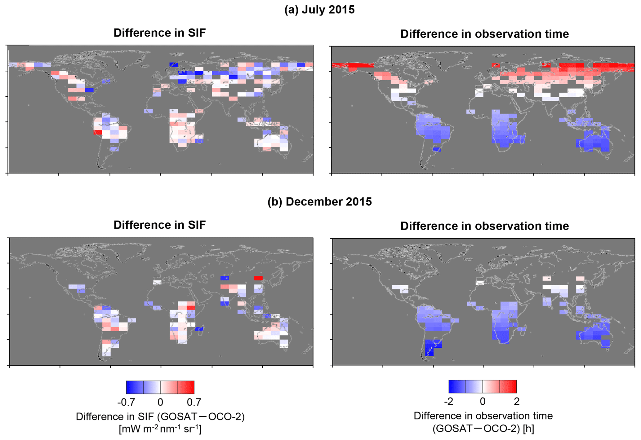
Figure 6 Difference in the monthly mean SIF (GOSAT – OCO-2) and difference in local time of the observation (GOSAT – OCO-2) within a 5^∘ × 10^∘ grid box: (a) July 2015; (b) December 2015. Only grids with more than nine data points are depicted.

Figure 7 shows that just such a lower GOSAT SIF was observed for the grids where there was a certain level of SIF emission (i.e. for areas that were not barren). Furthermore, the tendency varied over the study years: the difference between GOSAT SIF and OCO-2 SIF was significant in 2015. This seems to correspond to the photosynthetic activity of vegetation in this region: the satellite-based GPP (Luo et al., 2018) and the Soil Moisture Active Passive (SMAP) L4 carbon product (Madani et al., 2017) indicate the possibility of lower photosynthetic activity in 2015 compared to 2016. Although the influence of the zero-level offset correction might play some role in this effect (e.g. the different tendency between the cropland and the grassland in the USA found in Case 2), it is inferred that the diurnal cycle of SIF yield was reflected in the difference between GOSAT SIF and OCO-2 SIF for the northern high-latitude region. This was supported by the results that a lower GOSAT SIF compared to the OCO-2 SIF was observed for other zero-level offset correction methods as described below, and the difference in SIF varied over the study years.

For the Southern Hemisphere in July and December, the difference between GOSAT SIF and OCO-2 SIF was close to 0 (Fig. 6). These results indicate the agreement between GOSAT SIF and OCO-2 SIF, since the effect of the different observation times was considered to be small due to the fact that the southern regions with large differences in observation time mainly consisted of barren areas with low SIF emission (Fig. 7). The aforementioned hypothesis does not explain the difference in SIF for areas with almost no SIF emission.

The difference in the monthly mean SIF between GOSAT and OCO-2 within a 5^∘ × 10^∘ grid box was averaged over the 20^∘ latitude bin (Fig. S16), and time-averaged values were calculated (Fig. 8). The finding that the difference in SIF was close to 0 indicates agreement between GOSAT SIF and OCO-2 SIF for the latitude zone of 0 to 40^∘ N where the difference in the observation time was small. This is also applicable to the Southern Hemisphere, as the GOSAT SIF that had a zero level similar to that of OCO-2 SIF did not show positive deviation. Most areas in the Southern Hemisphere, where the difference in the observation time was large, mainly consisted of barren areas with low SIF emission. In the northern high-latitude region, the difference in the observation time and the characteristics of the vegetation seemed to result in a lower GOSAT SIF than OCO-2 SIF, although errors in the zero-level offset might be included. Interpreting the time-averaged results (Fig. 8) from the above point of view, we conclude that the GOSAT SIF is highly consistent with the OCO-2 SIF, with an averaged difference within 0.05 mW m⁻² nm⁻¹ sr⁻¹ and a month-to-month variation of about 0.05 mW m⁻² nm⁻¹ sr⁻¹. When confirming the difference in SIF for each month (Fig. S16), the difference varied around 0 with almost no clear seasonal cycle. The mean difference was within 0.1 mW m⁻² nm⁻¹ sr⁻¹ for most months and the variation between grids was about 0.2 mW m⁻² nm⁻¹ sr⁻¹. It should be noted that a somewhat large difference occurred in the latitude region where the difference in observation time was small, and a slight seasonal cycle remained for 40 to 60^∘ N.

SIF of 0.1 mW m⁻² nm⁻¹ sr⁻¹ corresponds to approximately 0.1 % of the TOA radiance. The difference in the observed TOA continuum radiance between GOSAT and OCO-2 is expected to be up to 5 % for the wavelength domain used (short-wavelength side of the O₂ A band) (Kataoka et al., 2017). These two facts do not contradict each other, since, in principle, SIF is determined with an error of noise level if the deviation of the spectra is caused by the radiance offset, and the radiance offset is perfectly corrected. Although the cause of the zero-level offset and its spatio-temporal variation were not fully elucidated, the retrievals and offset corrections for GOSAT and OCO-2 seemed to be nearly ideal, and then the sophisticated comparisons allowed us to confirm the good consistency between the SIFs.

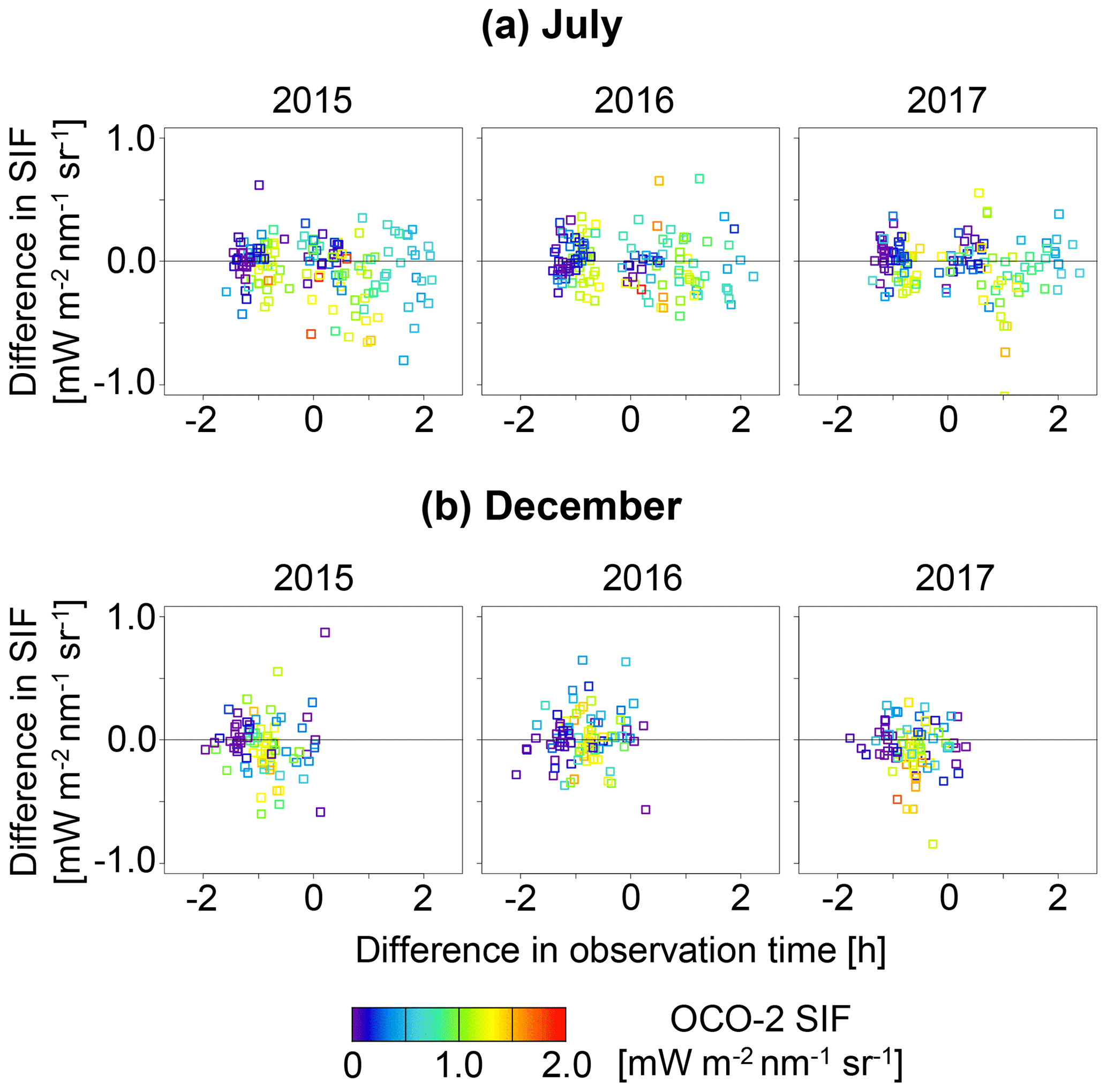
Figure 7 Relationship between the difference in SIF (GOSAT – OCO-2) and the difference in local time of the observation for 2015 to 2017: (a) July; (b) December. Each symbol represents a 5^∘ × 10^∘ grid box.

Zero-level offset was evaluated from bare soil data in the present study. On the whole, the results barely changed when different offset correction methods were used, but slight differences were found (Figs. S16 to S19). There is a possibility that the zero-level offset differs among land cover types or regions, and bare soil is suitable to the correction for land areas. More detailed investigation of the distribution of the filling-in signal according to land cover types and regions, including the difference between land and ocean, will be needed in the future. GOSAT SIF was lower than OCO-2 SIF for the northern high-latitude regions even for the zero-level offset correction using various vegetation-free targets that seem to give rise to positive bias (Figs. S17 and S18), supporting the hypothesis that characteristics of the vegetation result in a difference in SIF. Concerning the offset correction using bare soil separately for the Northern Hemisphere and the Southern Hemisphere, the narrow coverage of the TANSO-FTS radiance level and the small number of data for the offset table yielded a larger mean difference and standard deviation compared to the offset correction using bare soil over the globe (Figs. S16 and S19). Although offset correction using bare soil over the globe seems to be suitable for deriving SIF, its coverage of the TANSO-FTS radiance level is limited. Therefore, latitudinal investigation of the filling-in signal over cloudy ocean is a possible option to support the retrieval of gas concentration. More specifically, the apparent zero-level offset value that is retrieved simultaneously with the gas concentration (Frankenberg et al., 2012) can be compared with the zero-level offset evaluated from the case over cloudy ocean.

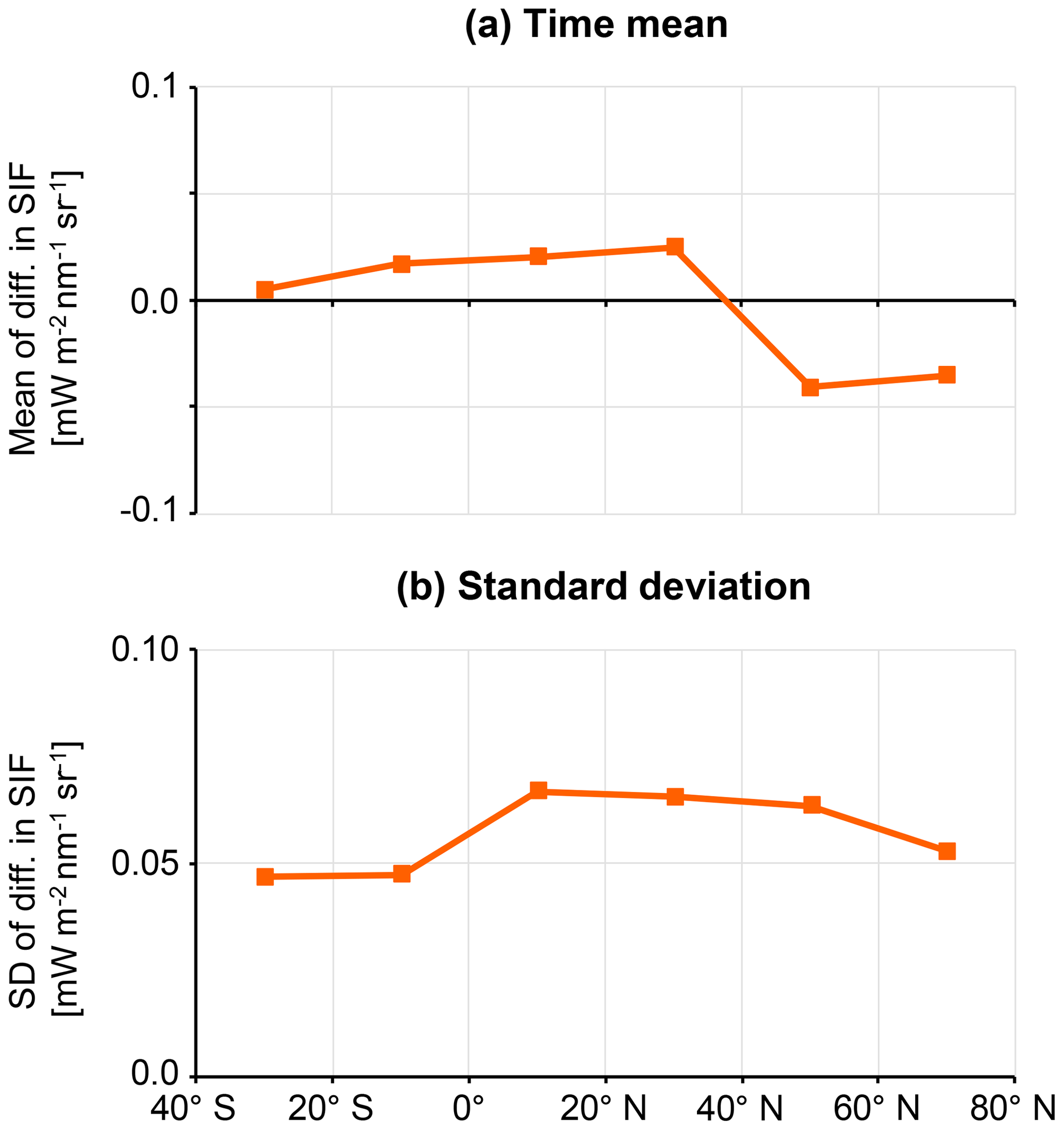
Figure 8 The monthly mean value shown in Fig. S16 is averaged over the target time period (February 2015 to January 2018): (a) averaged value; (b) standard deviation.

5 Conclusions

The difference in the filling-in signal among data identified by various criteria was analysed for the zero-level offset correction to derive SIF from the GOSAT TANSO-FTS spectra. Bare soil data should be identified by the criteria based on the albedo of the TANSO-FTS bands 2 and 3 and the NDVI value. The instrumental status is reflected in the temporal variation of the zero-level offset, indicating a need for re-evaluation of the radiometric degradation in the TANSO-FTS after switching the optics path selector. The zero-level offset correction was conducted, and the derived SIF was compared with OCO-2 SIF. GOSAT SIF generally agrees with OCO-2 SIF over areas with various SIF emissions, according to the comparison at the footprint level and in the specific vegetated regions with similar observation times. According to the investigation of the difference between GOSAT SIF and OCO-2 SIF within a 5^∘ × 10^∘ grid box over the globe, the GOSAT SIF was highly consistent with OCO-2 SIF, with a difference within 0.1 mW m⁻² nm⁻¹ sr⁻¹ for most months and a variation among grids of about 0.2 mW m⁻² nm⁻¹ sr⁻¹. The difference was 0.05 mW m⁻² nm⁻¹ sr⁻¹ for the temporal average.

Previous studies reported that the SIFs were consistent between GOME-2 and OCO-2, between TROPOMI and OCO-2, and between TanSat and OCO-2, while considering influential factors such as the observation time, location of the footprint, observation geometry, and wavelength. The comparison for GOME-2 was limited to the Amazon region, and the comparisons for TROPOMI and TanSat were initial-phase comparisons (Köhler et al., 2018a, b; Du et al., 2018). The present study compared GOSAT SIF and OCO-2 SIF under conditions in which the wavelength was similar between the sensors, cloudy data were excluded using the TANSO-CAI data for GOSAT, and the land cover type and LAI within the TANSO-FTS footprint were taken into account. The comparison was conducted at multiple spatial scales to take into account the difference in the observation pattern between the satellites. The GOSAT SIF agreed with the OCO-2 SIF, which was comparable to the findings of the aforementioned studies. Our results support the consistency among the present satellite-derived SIF data. It is also important that the consistency was confirmed between the FTS-derived and the grating spectrometer-derived SIF. Further studies will be needed to address the remaining bias, which seems to consist of instrumental effects, retrieval error, and characteristics of vegetation.