the Creative Commons Attribution 4.0 License.
the Creative Commons Attribution 4.0 License.
 | 11 Feb 2019
Development of a general calibration model and long-term performance evaluation of low-cost sensors for air pollutant gas monitoring
Rebecca Tanzer
Aliaksei Hauryliuk
Sriniwasa P. N. Kumar
Naomi Zimmerman
Levent B. Kara
Albert A. Presto
R. Subramanian
Assessing the intracity spatial distribution and temporal variability in air quality can be facilitated by a dense network of monitoring stations. However, the cost of implementing such a network can be prohibitive if traditional high-quality, expensive monitoring systems are used. To this end, the Real-time Affordable Multi-Pollutant (RAMP) monitor has been developed, which can measure up to five gases including the criteria pollutant gases carbon monoxide (CO), nitrogen dioxide (NO2), and ozone (O3), along with temperature and relative humidity. This study compares various algorithms to calibrate the RAMP measurements including linear and quadratic regression, clustering, neural networks, Gaussian processes, and hybrid random forest–linear regression models. Using data collected by almost 70 RAMP monitors over periods ranging up to 18 months, we recommend the use of limited quadratic regression calibration models for CO, neural network models for NO, and hybrid models for NO2 and O3 for any low-cost monitor using electrochemical sensors similar to those of the RAMP. Furthermore, generalized calibration models may be used instead of individual models with only a small reduction in overall performance. Generalized models also transfer better when the RAMP is deployed to other locations. For long-term deployments, it is recommended that model performance be re-evaluated and new models developed periodically, due to the noticeable change in performance over periods of a year or more. This makes generalized calibration models even more useful since only a subset of deployed monitors are needed to build these new models. These results will help guide future efforts in the calibration and use of low-cost sensor systems worldwide.
- Article
(1765 KB) - Full-text XML
-
Supplement
(4389 KB) - BibTeX
- EndNote


Current regulatory methods for assessing urban air quality rely on a small network of monitoring stations providing highly precise measurements (at a commensurately high setup and operating cost) of specific air pollutants (e.g., Snyder et al., 2013). The United States Environmental Protection Agency (EPA) determines compliance with national air quality standards at the county level using data collected by local monitoring stations. Many rural counties have at most a single monitoring site; urban counties may be more densely instrumented, though not at the neighborhood scale. For instance, the Allegheny County Health Department (ACHD) maintains a network of 10 monitoring stations which collect continuous and/or 24 h data for the 2000 km2 Allegheny County (with a population of 1.2 million) in Pennsylvania, USA, with only one of these stations providing continuous data for all EPA criteria pollutants listed in the National Ambient Air Quality Standards (NAAQS) (Hacker, 2017). However, air pollutant concentrations can vary greatly even within urban areas due to the large number and variety of sources (Marshall et al., 2008; Karner et al., 2010; Tan et al., 2014). This variability could lead to inaccurate estimates of air quality based on these sparse monitoring data (Jerrett et al., 2005).
One approach to increasing the spatial resolution of air quality data is the use of dense networks of low-cost sensor packages. Low-cost monitors are instruments which combine one or more comparatively inexpensive sensors (typically electrochemical or metal oxide sensors) with independent power sources and wireless communication systems. This allows larger numbers of monitors to be employed at a cost similar to that of a more traditional monitoring network as described above. The general goals of low-cost sensing include supplementing existing regulatory networks, monitoring air quality in areas that have lacked this in the past (for example in developing countries), and increasing community involvement in air quality monitoring through the provision of sensors and the resulting data to community volunteers to support more informed public decision-making and engagement in air quality issues (Snyder et al., 2013; Loh et al., 2017; Turner et al., 2017). Several pilot programs of low-cost sensor network deployment have been attempted, in Cambridge, UK (Mead et al., 2013); Imperial Valley, California (Sadighi et al., 2018; English et al., 2017); and Pittsburgh, Pennsylvania (Zimmerman et al., 2018).
There are several trade-offs resulting from the use of low-cost sensors. These sensors are less precise and sensitive than regulatory-grade instruments at typical ambient concentrations due to cross-sensitivities to other pollutants and dependence of the sensor response to ambient temperature and humidity (Popoola et al., 2016). These interactions are often nonlinear, meaning that linear regression models developed under controlled laboratory conditions are often insufficient to accurately translate the raw sensor responses into concentration measures (Castell et al., 2017). Due to the variety of interactions and atmospheric conditions which can affect sensor performance, covering the range of conditions to which the sensor will be exposed using laboratory calibrations is difficult. Field calibrations of the sensors are thus necessary, with the sensors being collocated with highly accurate regulatory-grade instruments. Various calibration methods that have been explored include the determination of sensor calibrations from physical and chemical principles (Masson et al., 2015), higher-dimensional models to capture nonlinear interactions (Cross et al., 2017), and nonparametric approaches including artificial neural networks (Spinelle et al., 2015) and k-nearest neighbors (Hagan et al., 2018). Recent work by our group compared lab-based linear calibration models with multiple linear regression and nonparametric random forest algorithms based on ambient collocations (Zimmerman et al., 2018). The machine learning algorithm using random forests on ambient collocation data enabled low-cost electrochemical sensor measurements to meet EPA data quality guidelines for hot spot detection and personal exposure for NO2 and supplemental monitoring for CO and ozone (Zimmerman et al., 2018).
There remain several unanswered questions with respect to the calibration of data collected by low-cost sensors which we seek to answer in this work by examining data collected by almost 70 Real-time Affordable Multi-Pollutant (RAMP) monitors over periods ranging up to 18 months in the city of Pittsburgh, PA, USA. First, although various models have been applied to perform calibrations in different contexts, a thorough comparison on a common set of data of several different forms of calibration models applied to multi-pollutant measurements has yet to be performed. We seek to provide such a comparison and thereby draw robust conclusions about which calibration approaches work best overall and in specific contexts. Second, in previous work with the RAMP monitors and in work with other sensors, unique models have been developed for each sensor. This requires that extensive collocation data be collected for each low-cost sensor, which may not be feasible if large sensor networks are to be deployed. Therefore, it is important to investigate how well a single generalized calibration model can perform when applied across different individual sensors. Third, it is important to quantify the generalizability of models calibrated using data collected at a specific location to other locations across the same city where the sensors might be deployed, which may not share the same ratios of pollutants. This question is examined with several RAMPs that are co-located with regulatory monitors in the city of Pittsburgh, PA, USA. Finally, we seek to address the stability of calibration models over time by tracking changes in performance over the course of a year, and from one year to the next. Overall, we find support for using a generalized model for a network of RAMPs, developed based on local collocation of a subset of RAMPs. This reduces the need to collocate each node of a network, which otherwise can significantly increase network operating costs. These results will help guide future deployment efforts for RAMP or similar lower-cost air quality monitors.
2.1 The RAMP monitor
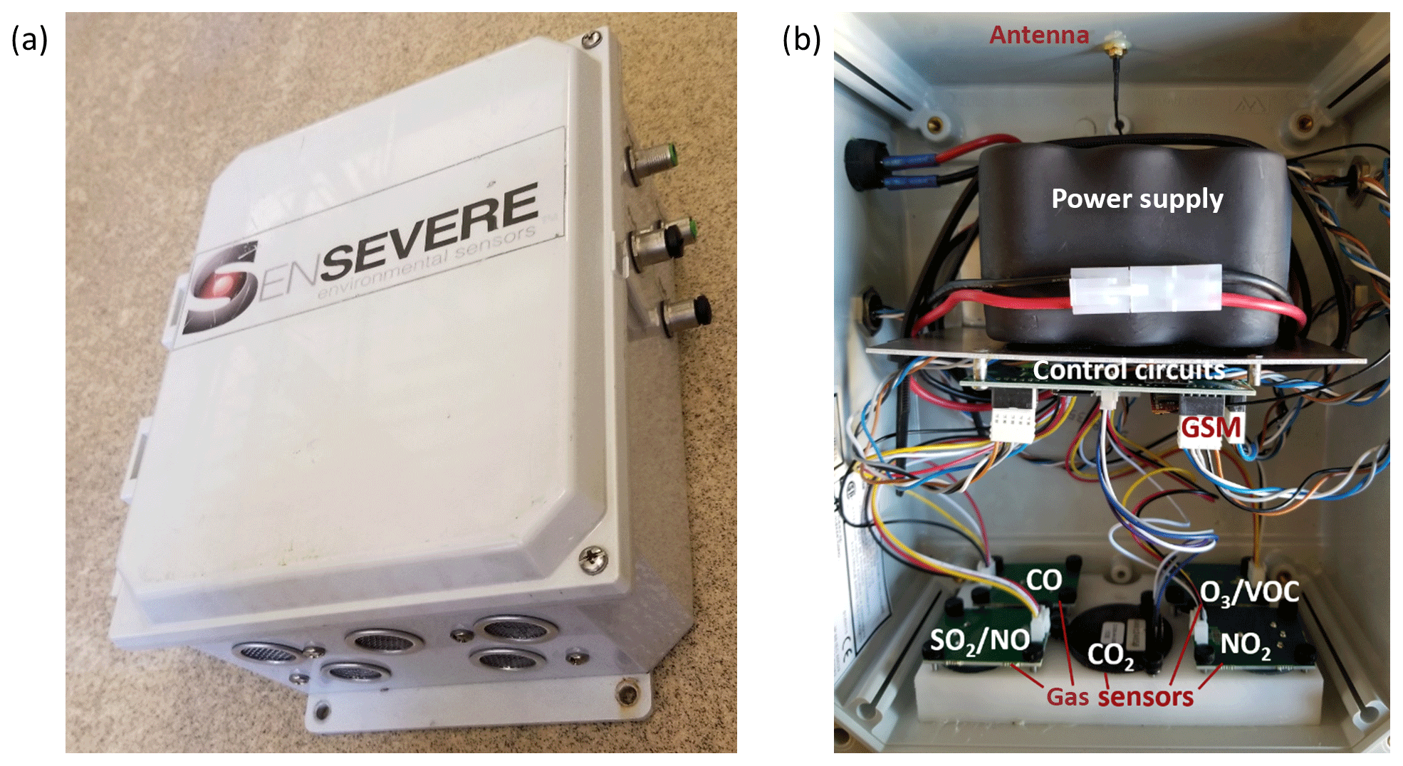
The RAMP monitor (Fig. 1) was jointly developed by the Center for Atmospheric Particle Studies at Carnegie Mellon University (CMU) and a private company, SenSevere (Pittsburgh, PA). The RAMP package combines a power supply, control circuitry, cellular network communications capability, a memory card for data storage, and up to five gas sensors in a weatherproof enclosure. All RAMPs incorporate a nondispersive infrared (NDIR) CO2 sensor produced by SST Sensing (UK), which also measures temperature and relative humidity (RH). All RAMPs have one sensor that measures CO and one sensor that measures NO2. Of the remaining sensors, one is either an SO2 or NO sensor, and the other measures a combination of either oxidants (referred to hereafter as an ozone or O3 sensor, since this is its primary function in the RAMP) or volatile organic compounds (VOCs). The VOC sensor is an Alphasense (UK) photoionization detector and all other unspecified sensors are Alphasense B4 electrochemical units. Specially designed signal processing circuitry ensures relatively low noise from the electrochemical sensors. Further details of the RAMP are provided elsewhere (Zimmerman et al., 2018). Data collected from a total of 68 RAMP monitors are considered in this work.
2.2 Calibration data collection
Following Zimmerman et al. (2018), RAMP monitors are deployed outdoors on a parking lot located on the CMU campus for a calibration based on collocated monitoring with regulatory-grade instruments. The parking lot (40∘26′31 N by 79∘56′33 W) is a narrow strip between a low-rise academic building to the south and several tennis courts to the north. RAMP monitors are deployed for 1 month or more to allow for exposure to a wide range of environmental conditions; in 2017, these deployments took place in the summer and fall. Less than 10 m from the RAMP monitors, a suite of high-quality regulatory-grade instruments, measuring ambient concentrations of CO (with a Teledyne T300U instrument), CO2 (LI-COR 820), O3 (Teledyne T400 photometric ozone analyzer), and NO and NO2 (2B Technologies model 405 nm) are stationed to provide true concentration values for these various gases to which the RAMP monitors are exposed. These regulatory-grade instruments are contained within a mobile laboratory van, into which samples are drawn through an inlet 2.5 m above ground level. Using sensor signal data collected by the RAMPs during this collocation period together with data collected by these regulatory-grade instruments, calibration models are created for each RAMP monitor prior to its deployment, as described in Sect. 2.3. Further details on the regulatory-grade instrumentation and the collocation process are provided in previous work (Zimmerman et al., 2018).
In addition to collocation at the CMU campus, additional special collocation deployments of RAMP monitors were performed, in order to allow independent comparisons between the RAMP monitor data and regulatory monitors at different locations. One RAMP monitor was collocated with ACHD regulatory monitors at their Lawrenceville site (40∘27′56 N by 79∘57′39 W), an urban background site where all NAAQS criteria pollutant concentrations are measured. The ACHD Parkway East site, located alongside the I-376 highway (40∘26′15 N by 79∘51′49 W), was chosen as an additional collocation site for observing higher levels of NO and NO2: up to ∼100 ppb for NO and ∼40 ppb for NO2. For reference, the NAAQS limit for 1 h maximum NO2 is 100 ppb (https://www.epa.gov/criteria-air-pollutants/naaqs-table, last access: 5 February 2019).
2.3 Gas sensor calibration models
Various computational models were applied to the sensor readings of the RAMPs (i.e., the net signal, or raw response minus reference signal, from each electrochemical gas sensor, together with the outputs of the CO2, temperature, and humidity sensor) to estimate gas concentrations, based entirely on ambient collocations of the RAMPs with regulatory-grade monitors. These models, outlined in the following subsections, include parametric models such as linear and quadratic regression models, a semi-parametric Gaussian process regression model, and nonparametric nearest-neighbor clustering, artificial neural network, and hybrid random forest–linear regression models. A common difficulty of nonparametric methods is generalizing beyond the training data set. For example, if no high concentrations are observed during the collocation period, then the resulting trained nonparametric model will be unable to estimate such high concentrations if it is exposed to these during deployment. This is of potential concern for air quality applications, as the detection of high concentrations is an important consideration. Parametric models avoid this difficulty, but at the cost of lower flexibility in the types of input–output relationships they can capture.
Models using each of these algorithms were calibrated in three separate categories. First, individualized RAMP calibration models (iRAMPs) were created for each RAMP, using only the data collected by gas sensors in that RAMP and the regulatory monitors. Individualized models are applied only to data from the RAMP on which they were trained. Second, from these individualized models, a best individual calibration model (bRAMP) was chosen, which performed best out of all the individualized models on a testing data set with respect to correlation (Pearson r; see Sect. 2.4). This model was then used to correct data from all other RAMPs which shared the same mix of gas sensors (to ensure that the inputs to the model would be consistent). Third, general calibration models (gRAMPs) were developed by taking the median of the data from a subset of the RAMP monitors deployed at the same place and time and treating this as a virtual “typical RAMP”, for which models were calibrated for each gas sensor (the median is used rather than the mean to reduce the effects of any erroneous measurements by a few gas sensors in some RAMP monitors on the typical signal). The motivation for the use of gRAMP models is similar to that of Smith et at. (2017); however, while in that work it is recommended that the median from a set of duplicate low-cost sensors be used to improve performance, in this work we use that method to develop the gRAMP calibration model but then apply this calibration to the outputs of individual sensors rather than to the median of a group of sensors. RAMPs were divided into training and testing sets for the gRAMP models randomly, with the caveat that the two RAMPs deployed to the Lawrenceville and Parkway East sites were required to be part of the testing set. Data from about three-quarters of the RAMP monitors (53 out of 68) were used for developing the general calibration models (although not all of these monitors were active at the same time). Data from the remaining 15 RAMP monitors were used for testing, ensuring that the testing data are completely distinct from the training data. For the gRAMP models, the set of possible model inputs was restricted to ensure that, for each gas, all necessary model inputs would be provided by every RAMP (e.g., for NO models, only CO, NO, NO2, T, and RH could be used as inputs since all RAMP monitors measuring NO would also measure these, but not necessarily any of the other gases). Thus, each of the calibration model algorithms was applied in three categories, yielding iRAMP, bRAMP, and gRAMP variants of each model. Finally, note that, for brevity, we will refer to iRAMP, bRAMP, or gRAMP model variants when discussing specific results; however, when drawing general conclusions about low-cost electrochemical gas sensor calibration methods, we will use less-RAMP-specific terms (such as “generalized models”).
In all cases, models were calibrated using training data, which consist of the RAMP monitor data collected during the collocation period (which are measurements of the input variables, i.e., the signals from the various gas sensors) together with the readings of the regulatory-grade instruments with which the RAMP monitor was collocated (which are the targets for the output variables). These collocation data are down-averaged from their original sampling rates to 15 min averages, to ensure stability of the trained models and minimize the effects of noise on the training process. From the collocation data, eight equally sized, equally spaced time intervals are selected to serve as training data for the calibration models. The number of training data is selected to be either 80 % of the collocation data or 4 weeks of data (corresponding to 2688 15 min averaged data points), whichever is smaller. The minimum number of training data is 21 days; if fewer are available, no iRAMP model is trained for this RAMP, and thus no iRAMP model performance can be assessed for it (although bRAMP and gRAMP models trained on other RAMPs are still applied to this RAMP for testing). Training data for gRAMP models are obtained in the same way, although in that case it is the data for the virtual typical RAMP which are divided, rather than data for individual RAMPs. Any remaining data from the collocation period are left aside as a separate testing set, on which the performance of the trained models is evaluated. Note that due to differences in which RAMPs and/or regulatory-grade instruments were operating at a given time, training and testing periods are not necessarily the same for all RAMPs and gases; for example, a certain time may be part of the training period for the CO model for one RAMP and be part of the testing period for the O3 model of another RAMP. However, the training and testing periods for a given RAMP and gas are always distinct. The division of data collected at the CMU site in 2017 into training and testing periods is illustrated in the Supplement (Figs. S6–S10). The division of data collected at the CMU site in 2016 is carried out in a similar manner. The choice of averaging period, of minimum and maximum training times, and of the method for dividing between training and testing periods is motivated by previous work with the RAMP monitors (Zimmerman et al., 2018). All data collected at sites other than the CMU site (i.e., the Lawrenceville or Parkway East sites) are reserved for testing; no training of calibration models is performed using data collected at these other sites, and so they represent a true test of the performance of the models at an “unseen” location.
2.3.1 Linear and quadratic regression models
Linear regression models represent perhaps the simplest and most common method for gas sensor calibration and have been used extensively in prior work (Spinelle et al., 2013, 2015; Zimmerman et al., 2018). A linear regression model (sometimes called a multi-linear regression model in the case that there are multiple inputs) describes the output as an affine function of the inputs. Here, linear functions are used where the sets of inputs are restricted to the signal of the sensor for the gas in question along with temperature and RH. For example, the calibrated measurement of CO from the RAMP, cCO, is an affine function of the signal of the CO sensor, sCO, and the temperature, T, and RH measured by the RAMP:
Coefficients αCO, αT, and αRH and offset term βCO are calibrated from training data to minimize the root-mean-square difference of cCO and the measured CO concentration from the regulatory-grade instrument. The one exception to this general formulation is for evaluation of , for which both and are used as inputs (along with T and RH); this is carried out to account for the fact that the sensor for O3 also responds to NO2 concentrations (Afshar-Mohajer et al., 2018).
In addition to linear regressions, quadratic regressions were also applied. These are the same as linear regressions but can involve second-order interactions of the input variables. For example, for CO, a quadratic regression function would be of the following form:
Note that, as above, a reduced set of inputs is used here. Quadratic regression models using such reduced sets (the same sets used for linear regression) are hereafter referred to as “limited” quadratic regression models; in contrast, models making full use of all available gas, temperature, and humidity sensor inputs from a given RAMP are referred to as “complete” quadratic regression models.
The main advantages of linear and quadratic regression models are their ease of implementation and calibration, as well as their ability to be readily interpreted, e.g., the relative magnitudes of the regression coefficients correspond to the relative importance of the different inputs in producing the output. The main disadvantage of these models is their inability to compute complicated relationships between input and output which are beyond that of a second-order polynomial. The training and application of linear and quadratic regression models are implemented using custom-written routines for the MATLAB programming language (version R2016b).
2.3.2 Gaussian process models
Gaussian processes are a form of regression which generalizes the multivariate Gaussian distribution to infinite dimensionality (Rasmussen and Williams, 2006). For the purposes of calibration, we make use of a simplified variant of a Gaussian process model. From the training data, both the signals of the RAMP monitors and the readings of the regulatory-grade instruments are transformed such that their distributions during the training period can be approximately modeled as standard normal distributions. This transformation is accomplished by means of a piecewise linear transformation, in which the domain is segmented and for each segment different linear mappings are applied. After this transformation, an empirical mean vector μ and covariance matrix Σ are computed for the regulatory-grade and RAMP measurements. The transformed measurements can then be described using a multivariate Gaussian distribution. For example, for a RAMP measuring CO, SO2, NO2, O3, and CO2, this distribution would be
where, for example, represents the concentration measurement for CO following the transformation. The mean vector and covariance matrix are divided as follows:
where μconc represents the mean of the (transformed) concentration measurements of the regulatory-grade instrument, μRAMP represents the mean of the (transformed) signal measurements from the RAMP, Σconc,conc represents the covariance of the (transformed) concentrations, ΣRAMP, RAMP represents covariance of the (transformed) RAMP signals, and Σconc, RAMP represents the covariance between the (transformed) concentrations and RAMP signals ( is the transpose of Σconc, RAMP). Once these vectors and matrices have been defined, the model is calibrated.
Given a new set of signal measurements from a RAMP, denoted as , these are transformed using the piecewise linear transformation defined above to give the set of transformed signal measures . These are then used to estimate the concentrations measured by the RAMP with the standard conditional updating formula of the multivariate Gaussian as follows:
The inverse of the original piecewise linear transformation is then applied to these transformed concentration estimates to yield the appropriate concentration estimates in their original units.
The main advantage of a Gaussian process calibration model of this form is its robustness to incomplete or inaccurate information; for example, if a signal from one gas sensor were missing or corrupted by a large voltage spike, in the former case the missing input could be “filled in” by the correlated measurements of other sensors, while in the latter case estimates would be “reigned in” by the more reasonable measures of the other sensors. A major disadvantage of this calibration model is its continued use of what is basically a linear regression formula, the only difference being in the nonlinear transformation from the original measurement space to the standard normal variable space used by the model. Furthermore, during the calibration process, the ratios of concentration for the pollutants of the collocation site may be learned by the model, making it less likely to predict differing ratios during field deployment. The training and application of Gaussian process calibration models are accomplished using custom-written routines in the MATLAB programming language.
2.3.3 Clustering model
The clustering model presented here seeks to estimate the outputs corresponding to new inputs by searching for input–output pairs in the training data for which the distance (by a predefined distance metric in a potentially high-dimensional space) between the new input and the training inputs is minimized and using the average of several outputs corresponding to these nearby inputs (the nearest neighbors). In a traditional k-nearest-neighbor approach, such as that used in previous work (Hagan et al., 2018), every input–output pair from the training data is stored for comparison to new inputs. Although this provides the best possible estimation performance via this approach, storing these data and performing these comparisons are computation- and memory-intensive. Therefore, in this work, the input data are first clustered, i.e., grouped by proximity of the input data. These clusters are then represented by their centroid, with the corresponding output being the mean of the outputs from the clustered inputs. In this work, training data are grouped into 1000 clusters using the “kmeans” function in MATLAB. Euclidian distance in the multidimensional space of the sensor signals from each RAMP is used. For estimation, the outputs of the five nearest neighbors to a new input are averaged.
A major advantage of this approach is its simplicity and flexibility, allowing it to capture complicated nonlinear input–output relationships by referring to past records of these relationships, rather than attempting to determine the actual pattern which these relationships follow. Such a method can perform very well when the relationships are stable, and when any new input with which the model is presented is similar to at least one of the inputs from the training period. However, as with all nonparametric models, generalizing beyond the training period is difficult, and the model will tend to perform poorly if the nearest neighbors of a new input are in fact quite far away, in terms of the distance metric used, from this input.
2.3.4 Artificial neural network model
The artificial neural network model, or simply neural network, is a machine learning paradigm which seeks to replicate, in a simplified manner, the functioning of an animal brain in order to perform tasks in pattern recognition and classification (Aleksander and Morton, 1995). A basic neural network consists of several successive layers of “neurons”. These neurons each receive a weighted combination of inputs from a higher layer (or the signal inputs, if they are in the top layer) and apply a simple but nonlinear function to them, producing a single output which is then fed on into the next layer. By including a variety of possible functions performed by the neurons and appropriately tuning the weights applied to inputs fed from one layer to the next, highly complicated nonlinear transformations can be performed in successive small steps.
Neural networks have been applied to a large number of problems, including the calibration of low-cost gas sensors (Spinelle et al., 2015). Neural networks represent an extremely versatile framework and are able to capture nearly any nonlinear input–output relationship (Hornik, 1991). Unfortunately, to do so may require vast numbers of training data, which it is not always practical to obtain. Calibration of these models is also a time-consuming process, requiring many iterations to tune the weightings applied to values passed from one layer to the next. In this work, neural networks were trained and applied using the “Netlab” toolbox for MATLAB (Nabney, 2002). The network has a single hidden layer with 20 nodes. To limit the computation time needed for model training, the number of allowable iterations of the training algorithm was capped at 10 000; this cap was typically reached during the training.
2.3.5 Hybrid random forest and linear regression models
A random forest model is a machine learning method which makes use of a large number of decision “trees”. These trees are hierarchical sets of rules which group input variables based on thresholding (e.g., the third input variable is above or below a given value). The thresholds used for these rules as well as the inputs they are applied to and the order in which they are applied are calibrated during training. The final groupings of input variables from the training data, located at the end or “leaves” of the branching decision tree, are then associated with the mean values of the output variables for this group (similar to a clustering model). For estimating an output given a new set of inputs, each decision tree within the random forest applies its sequence of rules to assign the new data to a specific leaf, and outputs the value associated with that leaf. The output of the random forest is the average of the outputs of each of its trees.
A primary shortcoming of the random forest model (which it shares with other nonparametric methods) is its inability to generalize beyond the range of the training data set, i.e., outputs of a random forest model for new data can only be within the range of the values included as part of the training data. For this reason, the standard random forest model was expanded into a hybrid random forest–linear regression model. The use of this approach for RAMP data was suggested by Zimmerman et al. (2018). Furthermore, it is similar to the approach of Hagan et al. (2018), who hybridize nearest-neighbor and linear regression models. In this modified model, a random forest is applied to new data to estimate the concentrations of various measured pollutants. For example, the concentration of CO measured by a RAMP including sensors for CO, SO2, NO2, O3, and CO2 is estimated using a random forest as
If this estimated concentration exceeds a given value (in this case, 90 % of the maximum concentration value observed during the training, corresponding to about 1 ppm in the case of CO), a linear model of the form of Eq. (1) is instead used to estimate the concentration. This linear model is calibrated using a 15 % subset of the training data with the highest concentrations of the target gas and is therefore better able to extrapolate beyond the upper concentration value observed during the training period. This hybrid model is therefore designed to combine the strengths of the random forest model, i.e., its ability to capture complicated nonlinear relationships between various inputs and the target output, with the ability of a simple linear model to extrapolate beyond the set of data on which the model is trained. Random forests are implemented using the “TreeBagger” function in MATLAB, and custom routines are used to implement hybrid models.
2.4 Assessment metrics
In the following section, the performance of the calibration models in translating sensor signals to concentration estimates is assessed in several ways. It should be noted that the metrics presented here are applied only for testing data, i.e., data which were not used to build the calibration models. Model performance on the training data is expected to be higher, and thus less representative of the true capability of the model. The estimation bias is assessed as the mean normalized bias (MNB), the average difference between the estimated and actual values, divided by the mean of the actual values. That is, for n measurements,
where cestimated,i is the measured concentration as estimated by the RAMP monitor and ctrue,i is the corresponding true value measured by a regulatory-grade instrument. The variance of the estimation is assessed via the coefficient of variation in the mean absolute error (CvMAE), the average of the absolute differences between the estimated and actual values divided by the mean of the actual values. The estimates used in evaluating the CvMAE are corrected for any bias as determined above:
where
Correlation between estimated and actual concentrations is assessed using the Pearson linear correlation coefficient (r):
where
and
Intuitively, these basic metrics are used to quantify the difference in averages between estimated and true concentrations (MNB), the average of differences between these (CvMAE), and the similarity in their behavior (r).
In addition to the above metrics, EPA methods for evaluating precision and bias errors are used as outlined in Camalier et al. (2007). To summarize, the precision error is evaluated as
where denotes the 10th percentile of the chi-squared distribution with n−1 degrees of freedom and the percent difference in the ith measurement is evaluated as
The bias error is computed as
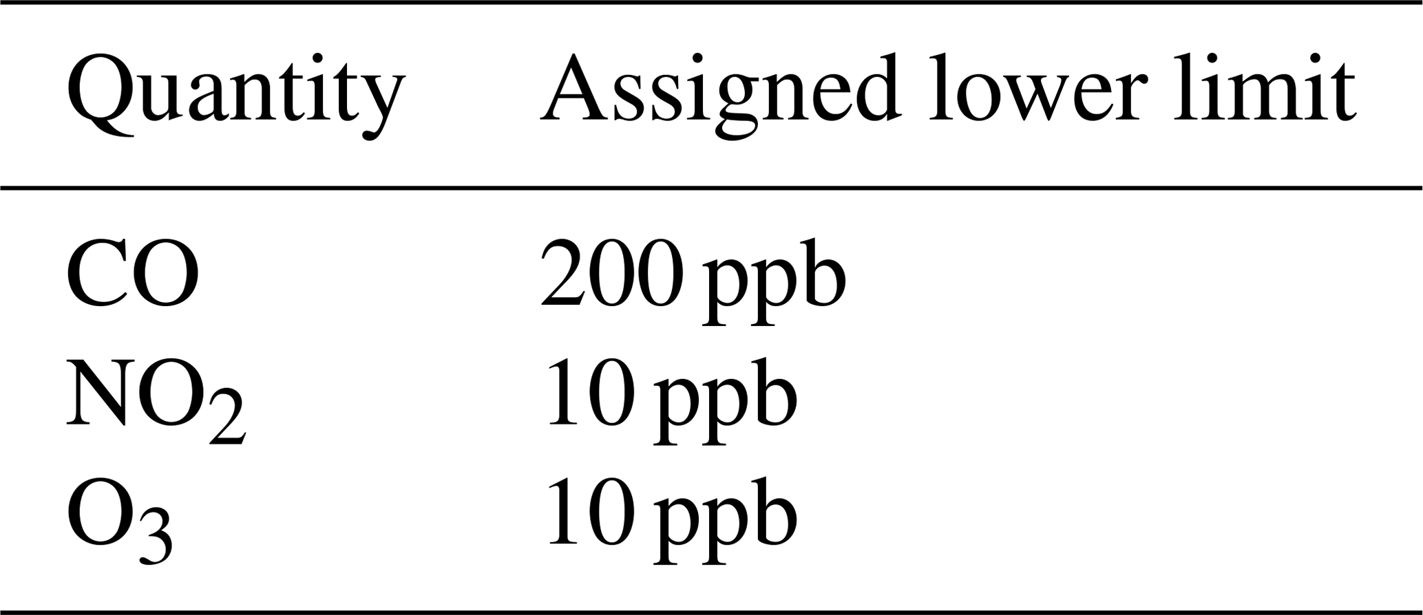
where is the 95th percentile of the t distribution with n−1 degrees of freedom. Prior to the computation of these precision and bias metrics, measurements for which the corresponding true value is below an assigned lower limit are removed from the measurement set to be evaluated, so as not to allow near-zero denominator values in Eq. (14). Lower limits used in this work are based on the guidelines presented by Williams et al. (2014) and are listed in Table 1. Note that this removal of low values is applied only when computing the precision and bias error metrics, and not when evaluating the other metrics described above.
Table 1Assigned lower limits for censoring small measurement values.
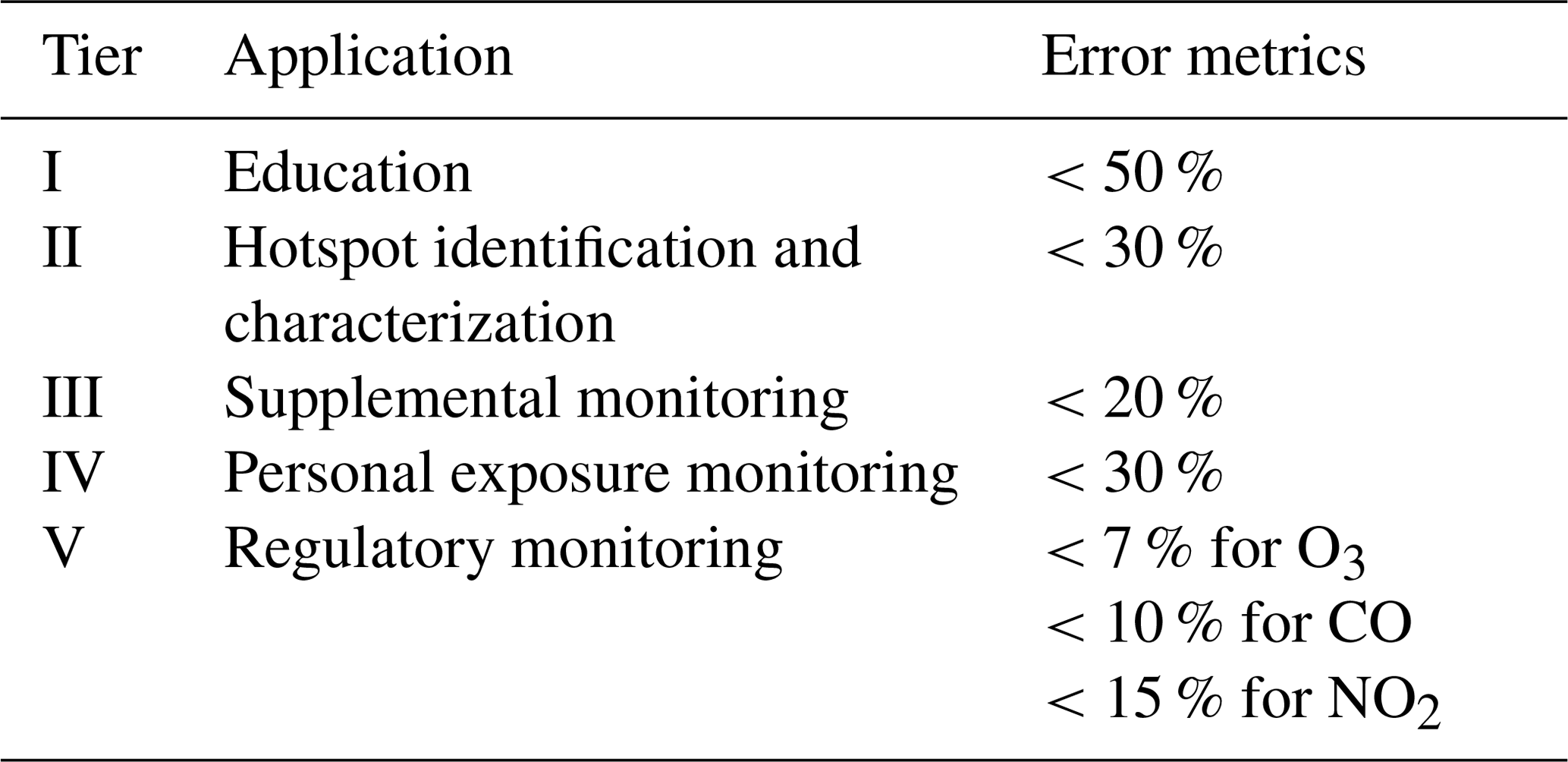
Using the EPA precision and bias calculations allows for these values to be compared against performance guidelines for various sensing applications, as presented in Williams et al. (2014) and listed in Table 2. For the RAMP monitors, a primary goal is to achieve data quality sufficient for hotspot identification and characterization (Tier II) or personal exposure monitoring (Tier IV), which requires that both precision and error bias metrics be below 30 %. A supplemental goal is to achieve performance sufficient for supplemental monitoring (Tier III), requiring precision and bias metrics below 20 %.
Table 2EPA air quality sensor performance guidelines for various applications. Reproduced from Williams et al. (2014).
In this section, we examine the performance of the RAMP gas sensors and the various calibration models applied to their data. We will focus our attention on the CO, NO, NO2, and O3 sensors. Results for calibration of measurements by the CO2 sensors are presented in the figures in the Supplement.
3.1 Performance across individualized models on CMU site collocation data
Figure 2 presents a comparison of the performance of various calibration models applied to testing data collected at the CMU site during 2017. As described in Sect. 2.3, collocation data are divided into training and testing sets, with the former (always being between 3 and 4 weeks in total duration) used for model development and the latter used to test the developed model using the assessment metrics described in Sect. 2.4, as presented in Fig. 2. All models in the figure are of the iRAMP category, being developed using only data collected by a single RAMP and the collocated regulatory-grade instruments. In the figure, squares indicate the median performance across all RAMPs for each performance metric, and the error bars span from the 25th to 75th percentiles of each metric across the RAMPs. For CO, 48 iRAMP models are compared; for NO, 19 models; for NO2, 62 models; and for O3, 44 models. Note that only 20 RAMP monitors included an NO sensor. An iRAMP model was not developed for RAMP monitors that had fewer than 21 days of collocation data with the relevant regulatory-grade instrument. The figures are arranged such that the lower-left corner denotes “better” performance (CvMAE close to 0 and r close to 1).

Figure 2Comparative performance of various individualized RAMP calibration models across gases measured by the RAMPs. Models are trained and tested on distinct subsets of collocation data collected at the CMU site during 2017; performance shown is based on the testing data set only. Proximity to the lower-left corner of each figure indicates better performance. Note the differing vertical axis scales.
Table 3Performance of iRAMP calibration models with respect to EPA air quality sensor performance guidelines as assessed at the CMU site. Entries in the table denote which models meet the corresponding guidelines for each gas (LR: linear regression; LQR: limited quadratic regression; CQR: complete quadratic regression; GP: Gaussian process; CL: clustering; NN: neural network; HY: hybrid random forest–linear regression).
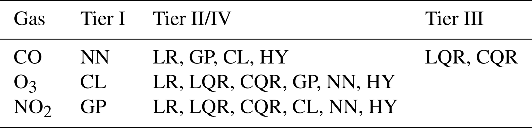
Typically, several of the model types provide similar performance for a given gas. For CO and O3, the simple parametric quadratic regression models perform as well as or better than the nonparametric modeling approaches, and even linear regression models give reasonable results. For NO2 and NO, while the nonparametric hybrid or neural network models perform best, complete quadratic regression models give comparable performance. Quadratic regression and hybrid models give the most consistently good performance, being among the top four methods across all gases. Bias tends to be low to moderate (depending on the gas) regardless of correction method (MNB less than 1 % for CO, less than 2 % for O3, less than 10 % for NO, and less than 20 % for NO2 across all methods). For the hybrid models, across gases, their random forest components were typically active from 88 % to 93 % of the time (or one crossing from random forest to linear models every 12 to 17 h of active sensor time), although for specific RAMPs this ranged from 75 % to 99 % (one “crossing” every 5 to 83 h) depending on the ranges of training and testing data. For perspective, the random forest component would be active 90 % of the time if the distributions of training and testing concentrations were identical. Table 2 lists the EPA performance guidelines for various applications, and Table 3 lists the modeling methods which meet these based on performance at the CMU site in 2017. All methods meet at least Tier I (educational monitoring, <50 % error) criteria for all gases considered. Most methods fall within the Tier II (hotspot detection) or Tier IV (personal exposure) performance levels (<30 % error) for all gases. For CO, quadratic regression methods meet Tier III (supplemental monitoring) criteria (<20 % error). In Table 4, the durations of the training and testing periods and the measured concentration ranges during these periods are provided. Finally, in Table 5, additional metrics about these performance results are presented, including un-normalized MAE and bias in the measured concentration units, to allow for direct comparison with the concentration ranges. More detailed information is also provided in the Supplement.
Table 4Durations and ranges of testing and training data at CMU in 2017. Durations of the training and testing periods are in days. Ranges indicated are in parts per billion for all gases, degrees Celsius for temperature (T), and percent for relative humidity (RH). Note that because training and testing periods vary for different RAMPs, as described in Sect. 2.3, the duration and concentration ranges of the training and testing periods will likewise vary. This table gives an indication of the variability in training and testing period durations across RAMPs, as well as the variability in concentrations, temperature, and relative humidity. The “lower range” indicates the variability in the lowest 15 min average concentration experienced by RAMPs during training or testing. Likewise, the “upper range” indicates the variability in the highest 15 min average concentrations. The “average range” indicates the variability in the average 15 min average concentration across RAMPs for either the training or testing period. Further information about these ranges is provided in the Supplement (see Figs. S11–S15).
Table 5Performance data for iRAMP models at CMU in 2017 (Avg. is the average; SD is the standard deviation). The “No.” sub-column under “Model” indicates the total number of iRAMP models developed for each gas. Slope and r2 are presented for the best-fit line between the calibrated RAMP measures and those of the regulatory monitor.

3.2 Comparison of individualized, best, and general models on CMU site collocation data
Next, we examine how the performance of the best individual models (bRAMP) and of the general models (gRAMP) applied to all RAMPs compare to the performance of the individualized RAMP (iRAMP) models presented in Sect. 3.1. Evaluation is carried out on the testing data collected at the CMU site in 2017. For simplicity, we restrict ourselves to three models for each gas, chosen from among the better-performing iRAMP models and including at least one parametric and one nonparametric approach. Figure 3 presents these comparisons.
Figure 3Comparative performance of individualized (iRAMP – square), best individual (bRAMP – diamond), and general (gRAMP – circle) model categories across gases measured by the RAMPs. The modeling algorithms used for each gas correspond to three of the better-performing algorithms identified among the individualized models. Models are trained and tested on distinct subsets of collocation data collected at the CMU site during 2017; performance shown is based on the testing data set only. Proximity to the lower-left corner of each figure indicates better performance.
Across all gases and models, iRAMP models tend to perform best, as might be expected since these models are both trained and applied to data collected by a single RAMP monitor, and therefore will account for any peculiarities of individual sensors. Between the bRAMP models, in which a model is trained using data from a single RAMP and applied across multiple RAMPs, and gRAMP models, which are trained on data from a virtual typical RAMP (composed of the median signal from several RAMPs) and then applied across other RAMPs, it is difficult to say which approach would be better based on these results, as they vary by gas as well as by modeling approach. For parametric models (i.e., linear and quadratic regression) the bRAMP and gRAMP versions typically have a similar performance, although there is less variability in performance for the gRAMP versions. For nonparametric models (i.e., neural network and hybrid models), performance of bRAMP versions is typically better than the gRAMP versions, although in the case of NO2 and O3 the performance is comparable. Overall, we find that a bRAMP or gRAMP version of several of the models can give similar performance to its iRAMP version, even though these models are not calibrated to each individual RAMP.
3.3 Performance of selected models at regulatory monitoring sites
Figure 4 depicts the performance of calibration models for two RAMP monitors deployed at two EPA monitoring stations operated by the ACHD (one monitor is deployed to each station). Filled markers indicate the performance of the models at these sites, while hollow markers indicate the 2017 testing period performance of the corresponding RAMP when it was at the CMU site for comparison. For each gas type, different calibration models are used, chosen from among the models depicted in Fig. 3. Models trained at the CMU site (as presented in previous sections) are used to correct data collected by the RAMP monitor at the station. Note that all data collected at either deployment site are treated as testing data, and that no data from these other sites are used to calibrate the models. Also note that not all gases monitored by RAMPs are monitored by the stations, hence why only one station may appear in each plot.

Figure 4Comparative performance of individual and general models for RAMPs deployed to ACHD monitoring stations (filled makers), compared to the performance of the same RAMPs at the CMU site (hollow markers). For example, a filled green marker indicates the performance of a RAMP at the Lawrenceville site, while a hollow green marker indicates the performance of that same RAMP when it was at the CMU site. The modeling algorithm used for each gas corresponds to the most consistent algorithm identified among the models depicted in Fig. 3: limited quadratic regression (LQR) for CO, neural network (NN) for NO, and hybrid random forest–linear regression models (HY) for NO2 and O3. Models are trained on data collected at the CMU site during 2017; performance shown for the CMU site (hollow marker) is based on the testing data for the corresponding RAMPs collected at that site. Proximity to the lower-left corner of each figure indicates better performance.
Overall, there tends to be a change in model performance at either of the deployment sites compared to the CMU site. This is to be expected to some degree, as the concentration range and mixture of gases (especially at the Parkway East site, which is located next to a major highway) can be different at a new site (where the model was not trained), and thus cross-sensitivities of the sensors may be affected. These differences appear to be greatest for CO, with performance being better at the Parkway East site, where overall CO concentrations are higher (both the average and standard deviation of the CO concentration at the Parkway East site are more than double those of the CMU or Lawrenceville sites). Additionally, gRAMP models tend to perform as well as or better than iRAMP models when monitors are deployed to new sites (only the CO results at Parkway East are much better for the iRAMP than the gRAMP models). Furthermore, the performance of the gRAMP models at the training site is typically more representative of the expected performance at other sites than that of the iRAMP models. This is likely because, while the iRAMP models are trained for individual RAMPs at the training site, the gRAMP models are trained across multiple RAMPs at that site, and therefore are more robust to a range of different responses for the same atmospheric conditions. Thus, when a RAMP is moved from one site to another, and its responses change slightly due to a change in the surrounding conditions, the gRAMP model will be more robust against these changes. Based on these results, since the change in performance as a monitor is deployed to a field site is often greater than the gap between iRAMP and gRAMP performance at the calibration site (as assessed in Sect. 3.2), there is no reason to prefer an iRAMP model to a gRAMP model for correction of field data.
To evaluate the performance of these sensors in a different way, EPA-style precision and bias metrics are provided in Fig. 5. Only CO, O3, and NO2 are considered, as these are the gases for which performance guidelines have been suggested by the EPA (Table 2). These guidelines are indicated by the dotted boxes in the figure; points falling within the box meet the criteria for the corresponding tier. Also, the range in observed performance at the CMU site, as depicted in Fig. 3, is reproduced here for comparison using black markers with error bars. For CO, by these criteria, the gRAMP model outperforms the iRAMP model, with the gRAMP model meeting Tier II or IV criteria (<30 % error) for all locations. Thus, under these metrics, for CO the gRAMP model is more representative of performance at other sites, while for the iRAMP model performance is more varied between sites. For O3, performance of both models at Lawrenceville is better than assessed at the CMU site, and both models fall near the boundary between Tiers II/IV and Tier III performance criteria (about 20 % error). For NO2, performance at the deployment sites in terms of the bias is always worse than predicted by the CMU performance, although in terms of precision, the gRAMP model at the CMU site better represents the site performance than the iRAMP model (the same trend as was seen using the other metrics).
Figure 5Comparative performance of individual and general models for RAMPs deployed to ACHD monitoring stations using EPA performance criteria. Dotted lines indicate the outer limits of each performance tier. Performance shown for the CMU site is based on performance across all RAMPs at that site based on testing data only. Proximity to the lower-left corner of each figure indicates better performance.
3.4 Performance of calibration models over time
We now examine the change in performance of calibration models over time. Figure 6 shows the performance of models developed based on data collected at the CMU site in both 2016 and 2017 and tested on data collected in either of these years.

Figure 6Comparative performance of models in 2016 and 2017. The “models” year indicates the year from which training data collected at the CMU site are used to calibrate the model; the “data” year indicates the year from which testing data collected at the CMU site are used to evaluate the model.
Training and testing data for 2017 represent the same training and testing periods as used for previous results. For 2016, training and testing data are divided using the same procedure as was applied for 2017 data, as discussed in Sect. 2.3. For example, the results for “2016 data, 2017 models” represent the performance of models calibrated using the training data subset of the 2017 CMU site data when applied to the testing data subset of the 2016 CMU site data. A change in performance between these two models on data from the same year will indicate the degree to which the models have changed from one year to the next; likewise, a change in performance for the same model applied to data from different years will indicate the degree to which sensor responses have changed over time. Note that NO is omitted here because data to build calibration models for this gas were not collected in 2016. Also note that results presented in the rest of this paper only use data collected in 2017 for model training and evaluation.
A drop in performance when models from one year are applied to data collected in the next year is consistently observed for all models and gases, with O3 having the smallest variability from one year to the next. This suggests that degradation is occurring in the sensors, reducing the intensity of their responses to the same ambient conditions and/or changing the relationships between their responses. Thus, a model calibrated on the response characteristics of the sensors in one year will not necessarily perform as well using data collected by the same sensors in a different year. This degradation has also been directly observed, as the raw responses of “old” sensors deployed with the RAMPs since 2016 were compared to those of “new” sensors recently purchased in 2018; in some cases, responses of old sensors were about half the amplitude of those of new sensors exposed to the same conditions. This is consistent with the operation of the electrochemical sensors, for which the electrolyte concentration changes over time as part of the normal functioning of the sensor. To compensate for this, new models should be calibrated for sensors on at least an annual basis, to keep track of changes in signal response. Furthermore, calibration models should preferably be applied to data from sensors with a similar age to avoid effects due to different signal responses of sensors which have degraded to varying degrees. Finally, in comparing model performance from one year to the next, there is no significant increase in error associated with using gRAMP models (trained for sensors of a similar age) rather than iRAMP or bRAMP models.
Additionally, calibration model performance was assessed as a function of averaging time. Note that the calibration models discussed in this paper are developed using RAMP data averaged over 15 min intervals, as discussed in Sect. 2.3. However, these models may be applied to raw RAMP signals averaged over longer or shorter time periods. Furthermore, the calibrated data can also be averaged over different periods. To investigate the effects of averaging time on calibration model performance, we assess the performance of RAMPs calibrated with gRAMP models for CO, O3, and CO2 at the CMU site in 2017, with averaging performed either before or after the calibration. Results are provided in the Supplement (Figs. S4 and S5). Overall, we find little variation in calibration model performance with respect to averaging periods between 1 min and 1 h.
3.5 Changes in field performance over time
Finally, we track the performance of RAMPs over time at specific deployment locations, as depicted in Fig. 7, to evaluate changes in calibration model field performance over time. This is carried out using three RAMP monitors; one was deployed at the ACHD Lawrenceville station from January through September of 2017, as well as during November and December 2017. A second RAMP was kept at the CMU site year-round, where it was collocated with regulatory-grade instruments intermittently between May and October. The third RAMP was deployed at the ACHD Parkway East site beginning in November of 2017. The same gRAMP calibration models as depicted in Fig. 4 (using the training data collected at the CMU site in 2017) are used; note that the RAMP present at the CMU site was a part of the training set of RAMPs for the gRAMP model, while the other two RAMPs were not. Performance of CO, NO2, and O3 sensors are depicted, as both CO and NO2 were continuously monitored at both ACHD sites and intermittently monitored at the CMU site, and O3 was consistently monitored at ACHD Lawrenceville as well as being intermittently monitored at the CMU site. Performance is assessed on a weekly basis. For CO, the limited quadratic regression gRAMP model is used, and for O3, the hybrid gRAMP model is used, as these showed the least variability in performance of the gRAMP models in Fig. 3. For NO2, a hybrid gRAMP model is used, which provided the same performance as the neural network gRAMP model in Fig. 3.
Figure 7Tracking the performance of RAMP monitors deployed to ACHD Lawrenceville, ACHD Parkway East, and CMU over time. Statistics are computed for each week. Results shown correspond to those of models trained using data collected at the CMU site during 2017. For CO, the generalized limited quadratic regression model is used; for NO2 and O3, generalized hybrid random forest–linear regression models are used.
Performance of the calibrated O3 measurements shows almost uniformly high correlation and low CvMAE throughout the year. For CO and (to a lesser degree) NO2, while CvMAE is relatively consistent, periods of lower and more variable correlation occurred from July to September (for CO) or October (for NO2). These periods of lower correlation do not appear to coincide with periods of atypical concentrations, periods of excessive pollutant variability at the site, or any unusual pattern in the other factors measured by the RAMP. Periods of lower performance appear to roughly coincide for the CMU and Lawrenceville sites for the time during which both sites were active, and observed pollutant concentration ranges were comparable for both the CMU and Lawrenceville sites during these periods. There does not appear to be a clear seasonal or temporal trend in this performance, as low correlations occur in the late summer but not early summer, when conditions were similar. Thus, while sensor performance is observed to fluctuate from week to week, there does not appear to be a seasonal degradation in performance.
Based on the results presented in Sect. 3.1, complete quadratic regression and hybrid models give the best and most consistent performance across all gases. Of these, the hybrid models, combining the complicated non-polynomial behaviors of random forest models (capable of capturing unknown sensor cross-sensitivities) with the generalization performance of parametric linear models, tend to generalize best for NO, NO2, and O3 when applied to data collected at new sites. For CO, quadratic regression models generalize better. Neural networks perform well for NO and NO2 but not for CO; limited quadratic regression models perform well for CO and O3 but not for NO and NO2. Linear regression, Gaussian processes, and clustering are the worst overall models for these gases, never being in the top two best-performing models, and only rarely being one of the top three. These results could perhaps be improved further; for instance, our linear and quadratic regression models did not use regularization, nor did we experiment with neural networks involving multiple hidden layers and varying numbers of nodes or with the use of different k means and nearest-neighbor algorithms for clustering.
Overall, in most cases the generic bRAMP and generalized gRAMP calibration models perform worse than the individualized iRAMP models at the calibration site, but the decline in performance may be manageable and acceptable depending on the use case. For example, for NO2 (Fig. 3), median performance of bRAMP and gRAMP neural network and hybrid models are only 15 % worse in terms of CvMAE and 5 % worse is terms of r. For O3, median performance of all models is above 0.8 for r and below 0.25 for CvMAE, indicating a high level of correlation and relatively low estimation error. For CO, limited quadratic models meet the same criteria. Furthermore, in examining the generalization performance of the models when applied to new sites, as depicted in Figs. 4 and 5, for NO2 (in terms of the r and CvMAE metrics) and for CO (in terms of the EPA precision and bias metrics), the gRAMP models show more consistent performance between the calibration and deployment locations than the iRAMP models. For O3, performance of iRAMP and gRAMP models at the Lawrenceville site is comparable, while for NO, performance of the gRAMP model at the Parkway East site is actually better than that of the iRAMP model. This may indicate that the NO sensors are more affected by changes in ambient conditions than the other electrochemical sensors, and the gRAMP model is better able to average out these sensitivities than the other model categories considered.
Based on comparisons between the performance of models from one year to the next, as well as the analysis of changes in performance of the RAMP monitors collocated with regulatory-grade instruments for long periods, some sensors, such as the O3 sensor, are quite stable over time. For the CO sensor, performance seemed variable over time, and performance noticeably degraded from one year to the next, although no seasonal trends were apparent, and overall performance may be acceptable (CvMAE < 0.5). The NO2 sensor also exhibited some degradation from one year to the next, although performance was stable over time in 2017, with minimal changes in overall performance during this long deployment period.
It can generally be expected that RAMP monitors will at least meet Tier II or Tier IV EPA performance criteria (<30 % error) for O3 (with hybrid random forest–linear regression bRAMP and possibly gRAMP models) and CO (with limited quadratic regression gRAMP models). Individualized calibration models are more likely to meet Tier II/IV criteria for NO2 (with iRAMP or bRAMP hybrid models), and localized calibration may also be required. For NO, while no specific target criteria are established, neural network iRAMP or gRAMP models appear to perform best.
Recommendations for future low-cost sensor deployments
In comparing different methods for the calibration of electrochemical sensor data, it was found that in some cases, e.g., for CO, simple parametric models, such as quadratic functions of a limited subset of the available inputs, were sufficient to transform the signals to concentration estimates with a reasonable degree of accuracy. For other gases, e.g., NO2, more sophisticated nonparametric models performed better, although parametric quadratic regression models making use of all sensor inputs were still among the best-performing models for all gases. Depending on the application, therefore, different methods might be appropriate, e.g., using simpler parametric models such as quadratic regression to calibrate measurements and provide real-time estimates, while using more sophisticated nonparametric methods such as random forest models when performing long-term analysis for exposure studies. Of the nonparametric methods considered, hybrid random forest–linear regression models gave the best general performance across all the gas types. These models, along with the quadratic models, should therefore be considered for situations in which it is desirable to use the same type of calibration across all gases, e.g., to reduce the “overhead” of programming multiple calibration approaches. The hybrid model, which combines the flexibility of the random forest with the generalizability of the linear model, is most theoretically promising for general application. Future work will also investigate other forms of hybrid models. For example, combinations of neural network and linear regression models may work well for NO, for which neural networks provided better performance than hybrid models using random forests. Also, for CO and ozone, hybrid models combining random forests with quadratic regression might perform better than those with linear models since quadratic models perform better than linear models for these gases overall.
Although there is a reduction in performance as a result of not using individualized monitor calibration models when these are calibrated and tested at the same location, the use of a single calibration model across multiple monitors, representing either the best of available individualized models or a general model developed for a typical monitor, tends to give more consistent generalization performance when tested at a new site. This suggests that variability in the responses of individual sensors for the same gas when exposed to the same conditions (such as would be accounted for when developing separate calibration models for each monitor) tends to be lower than the variability in the response of a single sensor when exposed to different ambient environmental conditions and a different mixture of gases (such as is experienced when the monitor is moved to a new site). Models that are developed and/or applied across multiple monitors will avoid “overfitting” to the specific response characteristics of a single sensor in a single environment. Thus, considering that it is impractical to perform a collocation for each monitor at the location where it is to be deployed, there is little benefit to developing individualized calibration models for each monitor when their performance will be similar to (if not worse than) that of a generalized model when the monitor is moved to another location.
There are several additional qualitative advantages to using generalized models. First, the effort required to calibrate models is reduced since not every monitor needs to be present for collocation and separate models do not have to be created for every monitor. For example, while for CO only 48 RAMPs had sufficient data to calibrate individualized models based on data collected at the CMU site in 2017, general models can be calibrated and applied for all 68 RAMPs which were at the CMU site during this period, as well as for additional RAMPs which were never collocated at the CMU site but have the same gas sensors installed. Second, collocation data collected from multiple monitors at different sites can be combined in the creation of a generalized model, whereas individualized models would require each monitor to be present at each collocation site. This means that a wider range of ambient gas concentrations can be reflected in the training data, allowing for better generalization. Finally, the use of generalized models allows for robustness against noise of individual sensors, which can lead to mis-calibration of individualized models but is less likely to do so if data from multiple sensors are averaged. Therefore, for future deployments, generalized models applicable across all monitors should be used.
For long-term deployments, it is recommended that model performance be periodically re-evaluated (using limited co-location campaigns with a subset of the deployed sensors) every 6 months to 1 year and that development of new calibration models be contingent on the outcomes of these re-evaluations. This recommendation is due to the noticeable change in performance when models for one year were used for processing data collected in the subsequent year. If generalized models are used, model development can be performed using only a representative subset of monitors collecting data across a range of temperature and humidity conditions, allowing most monitors to remain deployed in the field (although periodic “sanity checks” should be made for field-deployment monitors to ensure all on-board sensors are operating properly). Another option is to maintain a few “gold standard” monitors collocated with regulatory-grade instruments year-round and to use these monitors for the development of generalized models to be used with all field-deployed monitors over the same period. Determination of how many monitors are necessary to develop a sufficiently robust generalized model is a topic of ongoing work.
All data (reference monitor data, RAMP raw signal data, calibrated RAMP data for both training and testing), and codes (in MATLAB language) to recreate the results discussed here are provided online at https://doi.org/10.5281/zenodo.1302030 (Malings, 2018a). Additionally, an abridged version of the data set (without the calibrated data or models, but still including the codes to generate these) is available at https://doi.org/10.5281/zenodo.1482011 (Malings, 2018b).
The supplement related to this article is available online at: https://doi.org/10.5194/amt-12-903-2019-supplement.
CM analyzed data collected by the RAMP sensors, implemented the calibration models, and primarily wrote the paper. CM, RT, AH, and SPNK deployed, maintained, and collected data from RAMP sensors and maintained regulatory-grade instruments at the CMU site. NZ provided data from RAMP sensors and regulatory-grade instruments from the CMU site collected in 2016. NZ and LBK aided with the design of random forest and neural network calibration models, respectively, and provided general advice on the paper. AAP and RS conceptualized the research, acquired funding, provided general guidance to the research, and assisted in writing and revising the paper.
The authors declare that they have no conflict of interest.
Funding for this study is provided by the Environmental Protection Agency
(assistance agreement no. 83628601) and the Heinz Endowment Fund (grant nos.
E2375 and E3145). The authors thank Aja Ellis, Provat K. Saha, and
S. Rose Eilenberg for their assistance with deploying and maintaining the
RAMP network and Ellis S. Robinson for assistance with the CMU collocation
site. The authors also thank the ACHD, including Darrel Stern and
Daniel Nadzam, for their cooperation and assistance with sensor
deployments.
Edited by: Jun
Wang
Reviewed by: two anonymous referees
Afshar-Mohajer, N., Zuidema, C., Sousan, S., Hallett, L., Tatum, M., Rule, A. M., Thomas, G., Peters, T. M., and Koehler, K.: Evaluation of low-cost electro-chemical sensors for environmental monitoring of ozone, nitrogen dioxide, and carbon monoxide, J. Occup. Environ. Hyg., 15, 87–98, https://doi.org/10.1080/15459624.2017.1388918, 2018.
Aleksander, I. and Morton, H.: An introduction to neural computing, 2nd Edn., International Thomson Computer Press, London, 1995.
Camalier, L., Eberly, S., Miller, J., and Papp, M.: Guideline on the Meaning and the Use of Precision and Bias Data Required by 40 CFR Part 58 Appendix A, U.S. Environmental Protection Agency, available at: https://www3.epa.gov/ttn/amtic/files/ambient/monitorstrat/precursor/07workshopmeaning.pdf (last access: 5 February 2019), 2007.
Castell, N., Dauge, F. R., Schneider, P., Vogt, M., Lerner, U., Fishbain, B., Broday, D., and Bartonova, A.: Can commercial low-cost sensor platforms contribute to air quality monitoring and exposure estimates?, Environ. Int., 99, 293–302, https://doi.org/10.1016/j.envint.2016.12.007, 2017.
Cross, E. S., Williams, L. R., Lewis, D. K., Magoon, G. R., Onasch, T. B., Kaminsky, M. L., Worsnop, D. R., and Jayne, J. T.: Use of electrochemical sensors for measurement of air pollution: correcting interference response and validating measurements, Atmos. Meas. Tech., 10, 3575–3588, https://doi.org/10.5194/amt-10-3575-2017, 2017.
English, P. B., Olmedo, L., Bejarano, E., Lugo, H., Murillo, E., Seto, E., Wong, M., King, G., Wilkie, A., Meltzer, D., Carvlin, G., Jerrett, M., and Northcross, A.: The Imperial County Community Air Monitoring Network: A Model for Community-based Environmental Monitoring for Public Health Action, Environ. Health Persp., 125, 074501, https://doi.org/10.1289/EHP1772, 2017.
Hacker, K.: Air Monitoring Network Plan for 2018, Allegheny County Health Department Air Quality Program, Pittsburgh, PA, available at: http://www.achd.net/air/publiccomment2017/ANP2018_final.pdf (last access: 17 August 2017), 2017.
Hagan, D. H., Isaacman-VanWertz, G., Franklin, J. P., Wallace, L. M. M., Kocar, B. D., Heald, C. L., and Kroll, J. H.: Calibration and assessment of electrochemical air quality sensors by co-location with regulatory-grade instruments, Atmos. Meas. Tech., 11, 315–328, https://doi.org/10.5194/amt-11-315-2018, 2018.
Hornik, K.: Approximation capabilities of multilayer feedforward networks, Neural Networks, 4, 251–257, https://doi.org/10.1016/0893-6080(91)90009-T, 1991.
Jerrett, M., Burnett, R. T., Ma, R., Pope, C. A., Krewski, D., Newbold, K. B., Thurston, G., Shi, Y., Finkelstein, N., Calle, E. E., and Thun, M. J.: Spatial Analysis of Air Pollution and Mortality in Los Angeles, Epidemiology, 16, 727–736, https://doi.org/10.1097/01.ede.0000181630.15826.7d, 2005.
Karner, A. A., Eisinger, D. S., and Niemeier, D. A.: Near-Roadway Air Quality: Synthesizing the Findings from Real-World Data, Environ. Sci. Technol., 44, 5334–5344, https://doi.org/10.1021/es100008x, 2010.
Loh, M., Sarigiannis, D., Gotti, A., Karakitsios, S., Pronk, A., Kuijpers, E., Annesi-Maesano, I., Baiz, N., Madureira, J., Oliveira Fernandes, E., Jerrett, M., and Cherrie, J.: How Sensors Might Help Define the External Exposome, Int. J. Env. Res. Pub. He., 14, 434, https://doi.org/10.3390/ijerph14040434, 2017.
Malings, C.: Supplementary Data for “Development of a General Calibration Model and Long-Term Performance Evaluation of Low-Cost Sensors for Air Pollutant Gas Monitoring”, Zenodo, https://doi.org/10.5281/zenodo.1302030, 2018a.
Malings, C.: Supplementary Data for “Development of a General Calibration Model and Long-Term Performance Evaluation of Low-Cost Sensors for Air Pollutant Gas Monitoring” (abridged version), Zenodo, https://doi.org/10.5281/zenodo.1482011, 2018b.
Marshall, J. D., Nethery, E., and Brauer, M.: Within-urban variability in ambient air pollution: Comparison of estimation methods, Atmos. Environ., 42, 1359–1369, https://doi.org/10.1016/j.atmosenv.2007.08.012, 2008.
Masson, N., Piedrahita, R., and Hannigan, M.: Quantification Method for Electrolytic Sensors in Long-Term Monitoring of Ambient Air Quality, Sensors, 15, 27283–27302, https://doi.org/10.3390/s151027283, 2015.
Mead, M. I., Popoola, O. A. M., Stewart, G. B., Landshoff, P., Calleja, M., Hayes, M., Baldovi, J. J., McLeod, M. W., Hodgson, T. F., Dicks, J., Lewis, A., Cohen, J., Baron, R., Saffell, J. R., and Jones, R. L.: The use of electrochemical sensors for monitoring urban air quality in low-cost, high-density networks, Atmos. Environ., 70, 186–203, https://doi.org/10.1016/j.atmosenv.2012.11.060, 2013.
Nabney, I.: NETLAB: algorithms for pattern recognitions, Springer, London, New York, 2002.
Popoola, O. A. M., Stewart, G. B., Mead, M. I., and Jones, R. L.: Development of a baseline-temperature correction methodology for electrochemical sensors and its implications for long-term stability, Atmos. Environ., 147, 330–343, https://doi.org/10.1016/j.atmosenv.2016.10.024, 2016.
Rasmussen, C. E. and Williams, C. K. I.: Gaussian processes for machine learning, MIT Press, Cambridge, Mass., 2006.
Sadighi, K., Coffey, E., Polidori, A., Feenstra, B., Lv, Q., Henze, D. K., and Hannigan, M.: Intra-urban spatial variability of surface ozone in Riverside, CA: viability and validation of low-cost sensors, Atmos. Meas. Tech., 11, 1777–1792, https://doi.org/10.5194/amt-11-1777-2018, 2018.
Smith, K. R., Edwards, P. M., Evans, M. J., Lee, J. D., Shaw, M. D., Squires, F., Wilde, S., and Lewis, A. C.: Clustering approaches to improve the performance of low cost air pollution sensors, Faraday Discuss., 200, 621–637, https://doi.org/10.1039/C7FD00020K, 2017.
Snyder, E. G., Watkins, T. H., Solomon, P. A., Thoma, E. D., Williams, R. W., Hagler, G. S. W., Shelow, D., Hindin, D. A., Kilaru, V. J., and Preuss, P. W.: The Changing Paradigm of Air Pollution Monitoring, Environ. Sci. Technol., 47, 11369–11377, https://doi.org/10.1021/es4022602, 2013.
Spinelle, L., Aleixandre, M., Gerboles, M., European Commission, Joint Research Centre and Institute for Environment and Sustainability: Protocol of evaluation and calibration of low-cost gas sensors for the monitoring of air pollution., Publications Office, Luxembourg, available at: http://dx.publications.europa.eu/10.2788/9916 (last access: 13 February 2018), 2013.
Spinelle, L., Gerboles, M., Villani, M. G., Aleixandre, M., and Bonavitacola, F.: Field calibration of a cluster of low-cost available sensors for air quality monitoring. Part A: Ozone and nitrogen dioxide, Sensor. Actuat. B-Chem., 215, 249–257, https://doi.org/10.1016/j.snb.2015.03.031, 2015.
Tan, Y., Lipsky, E. M., Saleh, R., Robinson, A. L., and Presto, A. A.: Characterizing the Spatial Variation of Air Pollutants and the Contributions of High Emitting Vehicles in Pittsburgh, PA, Environ. Sci. Technol., 48, 14186–14194, https://doi.org/10.1021/es5034074, 2014.
Turner, M. C., Nieuwenhuijsen, M., Anderson, K., Balshaw, D., Cui, Y., Dunton, G., Hoppin, J. A., Koutrakis, P., and Jerrett, M.: Assessing the Exposome with External Measures: Commentary on the State of the Science and Research Recommendations, Annu. Rev. Publ. Health, 38, 215–239, https://doi.org/10.1146/annurev-publhealth-082516-012802, 2017.
Williams, R., Vasu Kilaru, Snyder, E., Kaufman, A., Dye, T., Rutter, A., Russel, A., and Hafner, H.: Air Sensor Guidebook, U.S. Environmental Protection Agency, Washington, DC, available at: https://cfpub.epa.gov/si/si_public_file_download.cfm?p_download_id=519616 (last access: 10 October 2018), 2014.
Zimmerman, N., Presto, A. A., Kumar, S. P. N., Gu, J., Hauryliuk, A., Robinson, E. S., Robinson, A. L., and R. Subramanian: A machine learning calibration model using random forests to improve sensor performance for lower-cost air quality monitoring, Atmos. Meas. Tech., 11, 291–313, https://doi.org/10.5194/amt-11-291-2018, 2018.