Filling the gaps of in situ hourly PM_2.5 concentration data with the aid of empirical orthogonal function analysis constrained by diurnal cycles

Data gaps in surface air quality measurements significantly impair the data quality and the exploration of these valuable data sources. In this study, a novel yet practical method called diurnal-cycle-constrained empirical orthogonal function (DCCEOF) was developed to fill in data gaps present in data records with evident temporal variability. The hourly PM_2.5 concentration data retrieved from the national ambient air quality monitoring network in China were used as a demonstration. The DCCEOF method aims to reconstruct the diurnal cycle of PM_2.5 concentration from its discrete neighborhood field in space and time firstly and then predict the missing values by calibrating the reconstructed diurnal cycle to the level of valid PM_2.5 concentrations observed at adjacent times. The statistical results indicate a high frequency of data gaps in our retrieved hourly PM_2.5 concentration record, with PM_2.5 concentration measured on about 40 % of the days suffering from data gaps. Further sensitivity analysis results reveal that data gaps in the hourly PM_2.5 concentration record may introduce significant bias to its daily averages, especially during clean episodes at which PM_2.5 daily averages are observed to be subject to larger uncertainties compared to the polluted days (even in the presence of the same amount of missingness). The cross-validation results indicate that our suggested DCCEOF method has a good prediction accuracy, particularly in predicting daily peaks and/or minima that cannot be restored by conventional interpolation approaches, thus confirming the effectiveness of the consideration of the local diurnal variation pattern in gap filling. By applying the DCCEOF method to the hourly PM_2.5 concentration record measured in China from 2014 to 2019, the data completeness ratio was substantially improved while the frequency of days with gapped PM_2.5 records reduced from 42.6 % to 5.7 %. In general, our DCCEOF method provides a practical yet effective approach to handle data gaps in time series of geophysical parameters with significant diurnal variability, and this method is also transferable to other data sets with similar barriers because of its self-consistent capability.

1 Introduction

A large variety of ground-based monitoring networks have been established worldwide to provide accurate measurements of various aspects of the atmospheric environment (Lolli and Di Girolamo, 2015). Many of these in situ measurements, however, suffer from data losses due to various unexpected reasons (e.g., instrumental malfunction, interruption of power supply, and internet outage), thus resulting in salient data gaps in the archived data records. Undoubtedly, these gaps significantly impair the data quality and the exploration of these valuable data sources. Therefore, filling data gaps present in such data sets is critical for the further exploitation of these in situ measurements.

Due to the high frequency and severity of haze pollution events, China started to establish the national ambient air quality monitoring network in 2012 by extending the range of the previous sparsely distributed monitoring network to cover most major Chinese cities. To date, more than 1600 state-controlled monitoring stations are routinely operated to measure concentrations of six primary air pollutants (i.e., PM₁₀, PM_2.5, O₃, NO₂, SO₂, CO) on an hourly basis (Guo et al., 2017; L. Li et al., 2017). These in situ measurements have been publicly released online via the China National Environmental Monitoring Center (CNEMC) in near real time as of 2013 but without the provision of any direct data download interface. Consequently, users oftentimes apply an automated software program (also known as a web crawler) to retrieve these valuable data sources from the CNEMC website. Such an endeavor empowers us to acquire hourly air quality data more efficiently.

As a critical air quality indicator, PM_2.5 mass concentration data have been widely used in many previous haze-related studies (Gao et al., 2018; Miao et al., 2018; Bai et al., 2019a, b; Zhang et al., 2019). Nevertheless, how data gaps were treated in the data exploration process (e.g., data integration and data transformation), especially for those using daily or monthly averaged PM_2.5 data sets (e.g., Guo et al., 2009; Miao et al., 2018; Ye et al., 2018; Zhang et al., 2018; Q. Yang et al., 2019), is oftentimes unclear. Since ignoring missing values would undoubtedly introduce biases into the final results (Bondon, 2005; Larose et al., 2019), some studies have attempted to perform data analysis on a relatively long timescale by integrating hourly records into a monthly resolution so as to mitigate the impacts of data gaps (e.g., Bai et al., 2019b; Zhang et al., 2019). On the other hand, many previous studies preferred to exclude records on days subject to a certain degree of missing values (e.g., no more than six missing values within 24 h) in their analysis (e.g., van Donkelaar et al., 2016; L. Li et al., 2017; Huang et al., 2018; Manning et al., 2018; Shen et al., 2018; Bai et al., 2019a; Zhang et al., 2019). Such a treatment of data gaps (e.g., ignoring missing values or excluding records on days with missingness) would either introduce new bias to the aggregated data record or make the original PM_2.5 time series temporally discontinuous, however.

Since a long-term PM_2.5 concentration record without gaps is essential to aerosol-related haze control and environmental health risk assessment (Yin et al., 2020), filling data gaps in the hourly PM_2.5 concentration record is of great value. Although there exist versatile gap-filling methods in the literature (e.g., Beckers and Rixen, 2003; Taylor et al., 2013; Chang et al., 2015; Dray and Josse, 2015; Gerber et al., 2018), most of them fail to properly restore missingness present in the data record with high temporal resolutions (e.g., hourly) and evident diurnal variability (e.g., PM_2.5 concentration), in particular the daily extrema. For instance, PM_2.5 concentrations vary significantly in space and time due to heterogeneous local emissions and atmospheric conditions (Guo et al., 2017; Lennartson et al., 2018; Shi et al., 2018). A similar barrier also applies to many other data sets which are sampled at a high temporal resolution. Therefore, a priori knowledge of the diurnal variation pattern of the analyzed data is vital to the restoration of missing values.

In this study, a novel yet practical gap-filling method called DCCEOF (that is, the diurnal-cycle-constrained empirical orthogonal function) was developed to better handle data gaps present in time series with marked variability in space and time, by taking the diurnal variation pattern as a critical constraint in missing-value prediction. To our knowledge, none of the existing gap-filling methods have accounted for the diurnal variation pattern of the given data in their missing-value restoration schemes, and hence the predicted values from such methods would be subject to large bias. As an illustration, the hourly PM_2.5 concentration record retrieved from CNEMC during the time period of 2014 to 2019 was applied to demonstrate the efficacy and accuracy of the suggested DCCEOF method. Scientific questions to be answered by this study include the following: (1) what is the frequency of data gaps shown in our retrieved in situ PM_2.5 record, (2) how many uncertainties can be introduced into PM_2.5 daily averages by missing values, (3) is it feasible to reconstruct the local diurnal variation pattern of PM_2.5 from discrete observations in the neighborhood, and (4) are missing values predicted by DCCEOF reliable?

2 Overview of existing gap-filling methods

Plenty of methods have been developed or adopted for gap filling with respect to various theoretical bases, ranging from simple replacement with surrogates (e.g., mean value) to spatiotemporal interpolation as well as complex machine learning techniques. Generally, these methods can be classified into different groups according to different criteria. For instance, two major groups can be classified based on the number of variables (univariate versus multivariate; Ottosen and Kumar, 2019) and the theoretical basis (likelihood-based versus imputation-based; Junger and Ponce de Leon, 2015). Table 1 summarizes a selection of popular gap-filling methods to deal with missingness in geophysical data sets according to the domain-specific data dependence (Gerber et al., 2018). Comparisons of the performance of these methods can also be found in other fields of literature, e.g., Kandasamy et al. (2013), Demirhan and Renwick (2018), Yadav and Roychoudhury (2018), and Julien and Sobrino (2019), to name a few.

Since each method is initially proposed to deal with missingness in one specific data set, adopting one method to use with another data set is often a challenge due to distinct features of missingness (e.g., missing at random versus missing not at random), in particular for data sets with significant spatiotemporal heterogeneity such as air pollutants time series (Junger and Ponce de Leon, 2015). PM_2.5 concentration often exhibits evident diurnal variation patterns, which are primarily governed by local air pollutant emissions and regional meteorological conditions such as boundary layer height (Guo et al., 2017, 2019; Z. Li et al., 2017; Huang et al., 2018; Liu et al., 2018; Miao et al., 2018; Yang et al., 2018; Y. Yang et al., 2019; Zhang et al., 2020). Consequently, conventional approaches like those listed in Table 1 may partially fail to accurately predict missing values in hourly PM_2.5 time series.

In general, most available gap-filling methods in Table 1 suffer from at least one of the following drawbacks: (1) partial failure for data sets with prominent gaps; (2) not self-consistent due to the requirement of supplementary data sets; (3) computationally intensive (e.g., neural networks); and, most critically, (4) unable to fairly predict daily peaks and/or minima due to the lack of essential prior knowledge of the diurnal variation cycle of monitoring targets. Given the significant heterogeneity of PM_2.5 concentration in space and time (Guo et al., 2017; Manning et al., 2018), ignoring the diurnal phases of PM_2.5 would result in large biases in the gap-filled PM_2.5 data set.

Table 1 Overview of several popular gap-filling methods to impute missingness in geophysical data sets.

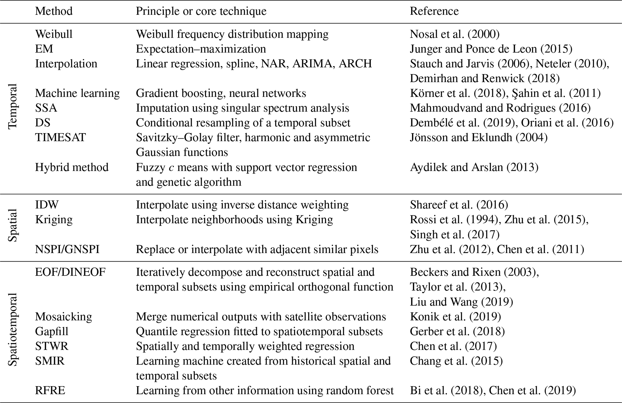
SSA: singular spectrum analysis; DS: direct sampling; IDW: inverse distance weighting; NSPI: neighborhood similar pixel interpolator; GNSPI: geostatistical neighborhood similar pixel interpolator; EOF: empirical orthogonal function; DINEOF: data interpolating empirical orthogonal function; STWR: spatially and temporally weighted regression; SMIR: smart information reconstruction; RFRE: random forest regression.

3 The DCCEOF gap-filling method

Given the significant heterogeneity of the PM_2.5 diurnal variation pattern associated with local emissions of air pollutants and atmospheric conditions, we propose incorporating the local diurnal variation pattern of PM_2.5 to constrain the prediction of missing values in each hourly PM_2.5 concentration record. The goal is to better predict missing PM_2.5 values, especially for the daily peaks and/or minima, which are poorly predicted by conventional methods due to the absence of prior knowledge of local diurnal phases of PM_2.5. Figure 1 presents a schematic illustration of the suggested DCCEOF method, which consists of the following four primary procedures toward the filling of data gaps present in each 24 h PM_2.5 time series.

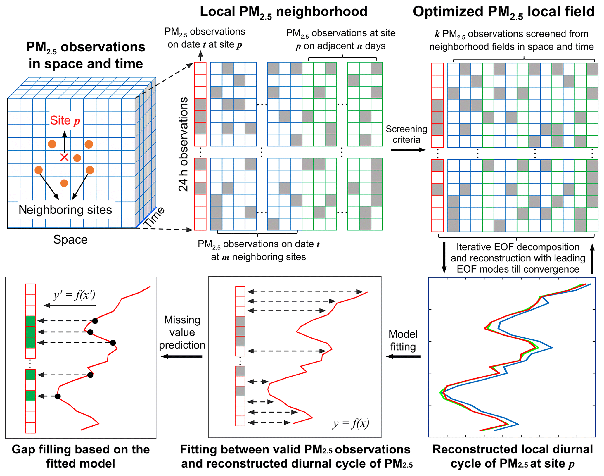
Figure 1 A schematic illustration of the suggested DCCEOF method to fill data gaps in hourly PM_2.5 concentration records. The grey squares denote missing values, while the ones outlined in green indicate restored data values.

(1) A local PM_2.5 neighborhood field is initialized: for a PM_2.5 missingness at site p on date t, an initial PM_2.5 neighborhood field in space and time (denoted as ${\mathbf{X}}_{p,t}^{m,n}$) was first constructed using 24 h PM_2.5 observations from nearby m stations on date t and adjacent 2n d (n days before and after t, respectively) at site p. Mathematically, the neighborhood field ${\mathbf{X}}_{p,t}^{m,n}$ can be expressed as

$$\begin{array}{}\text{(1)}& \begin{array}{rl}{\mathbf{X}}_{p,t}^{m,n}& =\left\{{\mathit{x}}_t^{\mathrm{1}},{\mathit{x}}_t^{\mathrm{2}},\mathrm{\dots },{\mathit{x}}_t^m,{\mathit{x}}_p^{t-n},\mathrm{\dots },{\mathit{x}}_p^{t-\mathrm{2}},{\mathit{x}}_p^{t-\mathrm{1}},{\mathit{x}}_p^{t+\mathrm{1}},\right.\\ & \left.{\mathit{x}}_p^{t+\mathrm{2}},\mathrm{\dots },{\mathit{x}}_p^{t+n}\right\}\end{array}.\end{array}$$

It is clear that m and n are two critical factors modulating the dimensions of ${\mathbf{X}}_{p,t}^{m,n}$. Considering a too-compact neighborhood field may be inadequate to reconstruct the local diurnal cycle of PM_2.5 fairly due to limited valid samples (because missingness may also emerge in each candidate 24 h PM_2.5 concentration record); here m was defined as the number of stations within 100 km (spatial window size) of the target station, while n was set to 7 (temporal window size) in our case. The spatial and temporal window sizes used here are based on our recent results in which an optimal window size of 50 km and 3 d was found to attain a good autocorrelation of PM_2.5 concentration in space and time, respectively (Bai et al., 2019c). To have adequate samples for the construction of ${\mathbf{X}}_{p,t}^{m,n}$, here we enlarged both the window sizes by simply doubling the values found in our previous study. These two window sizes would have little effect on the performance of the subsequent gap filling once they are large enough (at least greater than the identified optimal window sizes) to cover most similar observations nearby. This is because a sorting scheme is further applied to the neighborhood field to pinpoint observations having similar diurnal variation pattern with the target station. In other words, the two window sizes used here are simply to include adequate samples while avoiding incorporating all available data for the subsequent data reconstruction, in particular those far away.

(2) A compact PM_2.5 neighborhood field is constructed: since the initial PM_2.5 neighborhood field ${\mathbf{X}}_{p,t}^{m,n}$ might include many irrelevant observations with distinct diurnal variation patterns due to large spatial and temporal window sizes, a compact neighborhood field needs to be constructed by only retaining observations that are highly related to the target PM_2.5 time series ${\mathit{x}}_p^t$ with respect to the diurnal variation pattern. Therefore, the covariance rather than correlation between the target time series ${\mathit{x}}_p^t$ and every candidate PM_2.5 time series in ${\mathbf{X}}_{p,t}^{m,n}$ was first calculated (weighted by the number of valid data pairs within 24 h). Subsequently, the candidate PM_2.5 time series were sorted in terms of the magnitude of covariances in descending order. Finally, the first k time series were retained to construct the optimized PM_2.5 neighborhood field $\widehat{{\mathbf{X}}^k}$ by complying with the criterion that there were at least five valid observations at each specific time from 00:00 to 23:00 CST. The aim was to avoid large bias in the subsequent diurnal cycle reconstruction using empirical orthogonal function (EOF) analysis, since large outliers might emerge at times without any valid observation. Mathematically, the process to construct $\widehat{{\mathbf{X}}^k}$ can be formulated as follows:

$$\begin{array}{}\text{(2)}& {\displaystyle }{C}_{x{}^{\prime }}=\mathrm{COV}\left({\mathit{x}}_p^t,\mathit{x}{}^{\prime }\mathrm{|}{\mathbf{X}}_{p,t}^{m,n}\right)\text{and}\text{(3)}& {\displaystyle }\widehat{{\mathbf{X}}^k}=\left\{{\mathit{x}}_{\mathrm{1}}{}^{\prime },{\mathit{x}}_{\mathrm{2}}{}^{\prime },\mathrm{\dots },{\mathit{x}}_k{}^{\prime }\mathrm{|}{C}_{{\mathit{x}}_k{}^{\prime }}<C_{{\mathit{x}}_{k-\mathrm{1}}{}^{\prime }}<\mathrm{\dots }<C_{{\mathit{x}}_{\mathrm{1}}{}^{\prime }}\right\},\end{array}$$

where x^′ denotes the 24 h time series of candidate PM_2.5 in ${\mathbf{X}}_{p,t}^{m,n}$ and COV is the covariance function.

(3) The local diurnal cycle of PM_2.5 is reconstructed: the diurnal cycle of PM_2.5 at site p on date t (denoted as ${\mathit{\beta }}_p^t)$ was then reconstructed from the optimized PM_2.5 neighborhood field $\widehat{{\mathbf{X}}^k}$ using EOF in an iterative process similar to that of the DINEOF method (Beckers and Rixen, 2003). In our suggested DCCEOF method, the target PM_2.5 time series at site p on date t (denoted as ${\mathit{x}}_p^t$) were also included to constrain the reconstruction of ${\mathit{\beta }}_p^t$, and the whole field can be denoted as $\stackrel{\mathrm{̃}}{\mathbf{X}}$:

$$\begin{array}{}\text{(4)}& \stackrel{\mathrm{̃}}{\mathbf{X}}=\left\{{\mathit{x}}_p^t,\widehat{{\mathbf{X}}^k}\right\}.\end{array}$$

In general, the EOF-based gap-filling process can be outlined as follows: (a) 20 % of valid PM_2.5 observations in $\stackrel{\mathrm{̃}}{\mathbf{X}}$ were first retained for cross validation, and then these data values were treated as gaps by replacing them with nulls (i.e., missing values); (b) given that a small number of missing values would not significantly influence the leading EOF mode for the original data set, we assigned a first guess (here we used the mean value of valid data on each specific date) to the data points where missing values were identified to initialize the EOF analysis; (c) EOF analysis was performed on the previously generated background field (that is, $\stackrel{\mathrm{̃}}{\mathbf{X}}$ with gaps are filled with the daily mean and denoted as $<\stackrel{\mathrm{̃}}{\mathbf{X}}>$) in a form of singular value decomposition (SVD), and then data values at missing-value points were replaced by the reconstructed values using the first EOF mode at the corresponding locations. These processes can be expressed as

$$\begin{array}{}\text{(5)}& {\displaystyle }\left[\mathbf{U},\mathbf{S},\mathbf{V}\right]=SVD\left(<\stackrel{\mathrm{̃}}{\mathbf{X}}>\right)\text{and}\text{(6)}& {\displaystyle }\mathbf{X}{}^{\prime }={\mathit{u}}_{\mathrm{1}}\times {\mathit{s}}_{\mathrm{1}}\times {\mathit{v}}_{\mathrm{1}},\end{array}$$

where $<\stackrel{\mathrm{̃}}{\mathbf{X}}>$ denotes the initial matrix in which the missing values were filled with daily means. U, S, and V are three matrices derived from SVD, while u₁, s₁, and v₁ denote the SVD components in the first EOF mode. X^′ is the reconstructed matrix using the first EOF mode; (d) the matrix was iteratively decomposed and reconstructed while data values at the missing-value points were updated using the first EOF mode till the convergence was confirmed by the mean square error at each iteration; (f) the above iterative processes were repeated by including the following EOF modes till the final convergence was reached (i.e., mean square error started to increase when a new EOF mode was included). The diurnal cycle ${\mathit{\beta }}_p^t$ was finally derived by standardizing the identified leading EOF modes in the last round iteration.

(4) Missing values are predicted: a linear relationship was then established between valid PM_2.5 observations in the original time series ${\mathit{x}}_p^t$ and the corresponding values in ${\mathit{\beta }}_p^t$. Missing values in ${\mathit{x}}_p^t$ were then predicted by mapping data values in the reconstructed diurnal cycle ${\mathit{\beta }}_p^t$ at missing times to the level of valid PM_2.5 observations based on the established linear relationship.

In short, our suggested DCCEOF method is a univariate and self-consistent gap-filling method since no additional data record is required for the restoration of missing values. Rather, the method works relying primarily on the local diurnal cycle of PM_2.5 that can be reconstructed from discrete PM_2.5 neighborhood fields in space and time. In contrast to conventional gap-filling methods that work on a purely statistical basis (e.g., spline interpolation), the unique feature and novelty of the suggested DCCEOF method lie in the accounting for the local diurnal variation pattern of the input data in their missing-value predictions, thus making the predicted values physically meaningful and highly accurate.

4 Case study

4.1 China in situ PM_2.5 concentration records

The near-surface mass concentration of PM_2.5 across China is measured primarily using the tapered element oscillating microbalance analyzer and/or the beta attenuation monitor at each monitoring station. The instruments' calibration, operation, maintenance, and quality control are all properly conducted by complying with the Chinese environmental protection standards GB 3095-2012 and HJ 618-2011. PM_2.5 concentration data are measured by these instruments with an accuracy of ±5 µg m⁻³ for 10 min averages and ±1.5 µg m⁻³ for hourly averages (Guo et al., 2017; Miao et al., 2018). Although the hourly PM_2.5 observations in China have been publicly available since 2013, the PM_2.5 records used in the present study have been retrieved since May 2014 via a web crawler program.

Figure 2 depicts the spatial distribution of monitors in the national ambient air quality monitoring network in China as well as the starting year of the release of PM_2.5 measurements to the public at each individual station. Given the fact that our data were retrieved after May 2014, stations deployed before that should hardly be separated from those operated from 2014, and hence, they were all designated in the same way in Fig. 2. At present, this network consists of more than 1600 stations, in which about 940 stations were established before 2015. The total number was increased to 1494 in June 2015, and then only four stations were newly deployed in the following 1.5 years till December 2016. In other words, the vast majority (92.4 %) of stations in the current network was deployed before the middle of 2015.

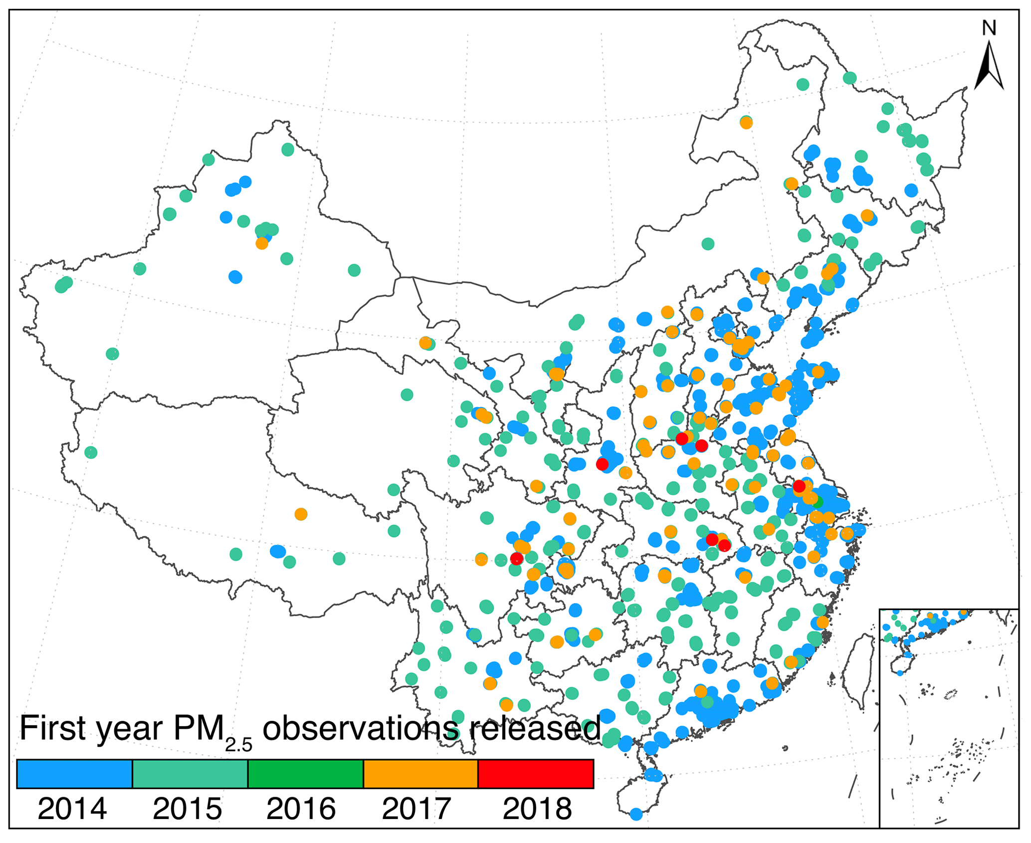
Figure 2 Spatial distribution of national ambient air quality monitoring network stations in China from May 2014 to April 2019. Circles with distinct color indicate the year in which the first PM_2.5 observation was publicly released in our retrieved data record.

4.2 Results

4.2.1 Data incompleteness of in situ PM_2.5 records in China

Figure 3a–c present the daily averaged missing-value ratio, the occurrence frequency of missingness (defined as the ratio of days with missing values in each 24 h of PM_2.5 observations divided by the total number of days), and the diurnal phases of the most frequently occurring missing values at each monitoring station since the first release of PM_2.5 observations to the public, while Fig. 3d–f show the corresponding histograms, respectively. Although most of the stations have a daily averaged missing-value ratio of less than 10 % (Fig. 3a and d), significant data gaps are still observed at several monitoring stations (red dots in Fig. 3a) with more than 70 % of hourly PM_2.5 observations lost in the daily 24 h measurements. After checking the retrieved PM_2.5 data records over these stations, we found that most of these stations stopped releasing PM_2.5 observations after the middle of 2015.

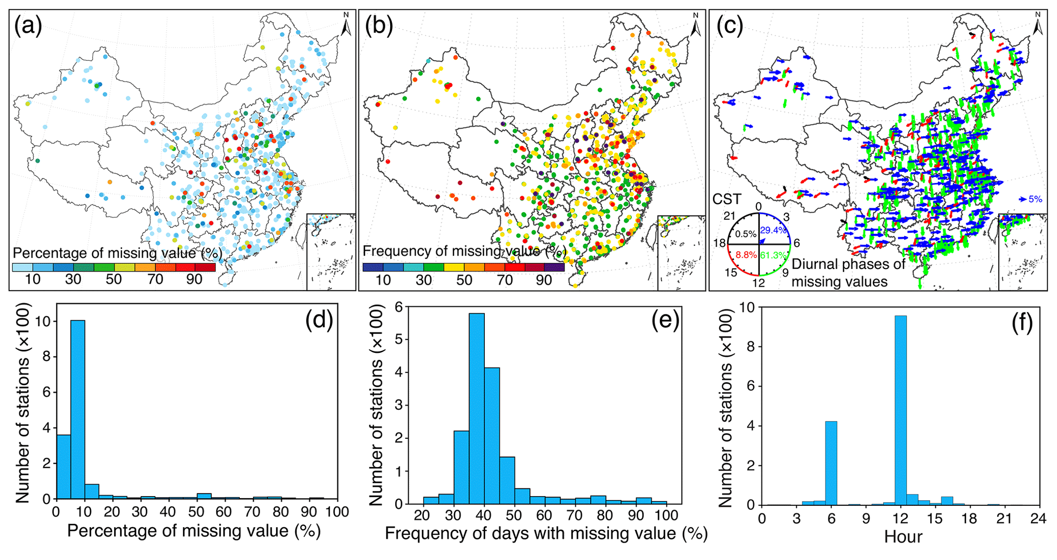
Figure 3 Statistics associated with missing values present in the site-specific hourly PM_2.5 concentration record since the time of the release of the first PM_2.5 observation onward. (a) Percentage of missingness in each PM_2.5 record, (b) frequency of days with missing values, (c) diurnal phases of the maximum frequency of missing values occurring within 24 h, (d–f) histograms for (a–c), respectively. The arrow direction in (c) indicates the local time (China standard time, CST) at which missing values occurred most frequently and the arrow length shows the magnitude of frequency. The varying diurnal phases of missing values are represented by different colors: blue (00:00–06:00 CST), green (06:00–12:00 CST), red (12:00–18:00 CST), and black (18:00–24:00 CST).

Despite the small magnitudes (∼10 %) of daily averaged missing-value ratios (Fig. 3d), data gaps in our retrieved hourly PM_2.5 record are still significant, which is evidenced by the occurrence frequency of missing values in daily PM_2.5 observations (Fig. 3b). In contrast to the daily averaged missing-value ratios (Fig. 3a), the frequency of days with missing values has a relatively larger magnitude of about 40 % (PM_2.5 data measured on 4 out of 10 d suffered from missingness), indicating an extraordinary high chance of suffering from data gaps in the retrieved PM_2.5 record (Fig. 3e). These results suggest an urgent need to fill data gaps in our retrieved PM_2.5 concentration record so as to facilitate the further exploration of this valuable data set.

Figure 3c presents the diurnal variation pattern of the occurrence of missingness in the retrieved PM_2.5 record in terms of the detailed time (represented by the arrow direction) and frequency (represented by the relative length of each arrow) of the most commonly occurring missing values, while Fig. 3f shows the histogram of the local time at which missing values occurred most frequently at each monitoring station. It is noteworthy that missing values occurred more frequently in the morning over most stations (90.7 % of total population of stations), particularly at 06:00 and 12:00 CST. Nevertheless, detailed reasons for this diurnal variation pattern remain unclear.

4.2.2 Impacts of data gaps on PM_2.5 daily averages

Given the common application of daily averaged PM_2.5 concentration data in many studies, the possible impacts of data gaps on PM_2.5 daily averages were assessed here to examine how well the estimated PM_2.5 daily averages can be trusted in the presence of data gaps, especially during different pollution regimes. Toward such a goal, gap-free observations of hourly PM_2.5 concentration within 24 h were first extracted. To make the computational workload manageable, we randomly sampled 1000 d of observations rather than using observations from all gap-free days. Moreover, days with a PM_2.5 daily average lower than that of the 10th percentile of all gap-free days were considered as the clean scenario, while those with an average greater than the 90th percentile were treated as the polluted scenario. Subsequently, a varying number (ranging from 1 to 23) of data values were selected and then treated as gaps in every 24 h of PM_2.5 observations randomly. Mean relative differences (MRDs) between PM_2.5 daily averages derived from hourly records with and without data gaps were finally calculated to examine the potential impacts of missingness on PM_2.5 daily averages.

Figure 4a shows the estimated MRDs at the 10th, 50th, and 90th percentiles associated with different numbers of missing values in each 24 h of PM_2.5 observations. There is no doubt that larger biases could be introduced into PM_2.5 daily averages with an increase in the total number of missingness. Given the symmetrical behavior of MRDs around zero (50th percentile) for each given number of missingness, we may infer that random biases could be introduced into PM_2.5 daily averages if missing values are ignored for the calculation of daily averages of PM_2.5. These random biases, in turn, could result in large uncertainties in the subsequent results such as trend estimations. To further evaluate the impacts of missingness on PM_2.5 daily averages, in particular at different pollution scenarios, MRDs were also calculated on 1000 clean and polluted days, respectively (Fig. 4b–d). On average, MRDs vary with larger deviations on clean days than polluted days (Fig. 4b). Regarding MRDs at the 10th and 90th percentiles, we may deduce that missing values would result in larger bias in PM_2.5 daily averages on clean days than in polluted conditions given the larger MRDs during clean scenarios (Fig. 4c–d). This effect is in line with expectations since PM_2.5 concentration often exhibits relatively larger diurnal variations on cleaner days than during polluted episodes due to the possible boundary layer height effect (Z. Li et al., 2017; Miao et al., 2018). Moreover, six missing values in 24 h of observations would result in as large as approximately 5 % of deviations (10 % for 12 missing values) from PM_2.5 daily averages during clean days (Fig. 4c–d).

In addition to the total number of missing values, possible impacts of diurnal phases of missing values on PM_2.5 daily averages were also examined. This analysis shows that different diurnal phases were observed for MRDs associated with missingness at different pollution levels (Fig. 5). Specifically, missing values in the afternoon and evening would be more likely to overestimate PM_2.5 daily averages, whereas an opposite effect (underestimations) was observed for missingness in the morning and at night. Moreover, the missingness in the afternoon during clean days has a larger potential to overestimate PM_2.5 daily averages than during other times. This effect could be largely associated with the diurnal phases of PM_2.5 as daily peaks are oftentimes observed in the early morning (Wang and Christopher, 2003), though such a diurnal variation pattern may differ by region (Lennartson et al., 2018). Also, the diurnal phases of PM_2.5 are largely dominated by the diurnal variation in regional emissions and boundary layer processes (Guo et al., 2016; Lennartson et al., 2018; Miao et al., 2018; Y. Yang et al., 2019). In contrast, the diurnal phases of MRDs are not evident during polluted days. The above findings collectively suggest the need to fill data gaps in hourly PM_2.5 observations, especially for those measured during clean days, since missing values would result in larger biases in PM_2.5 daily averages than during polluted episodes.

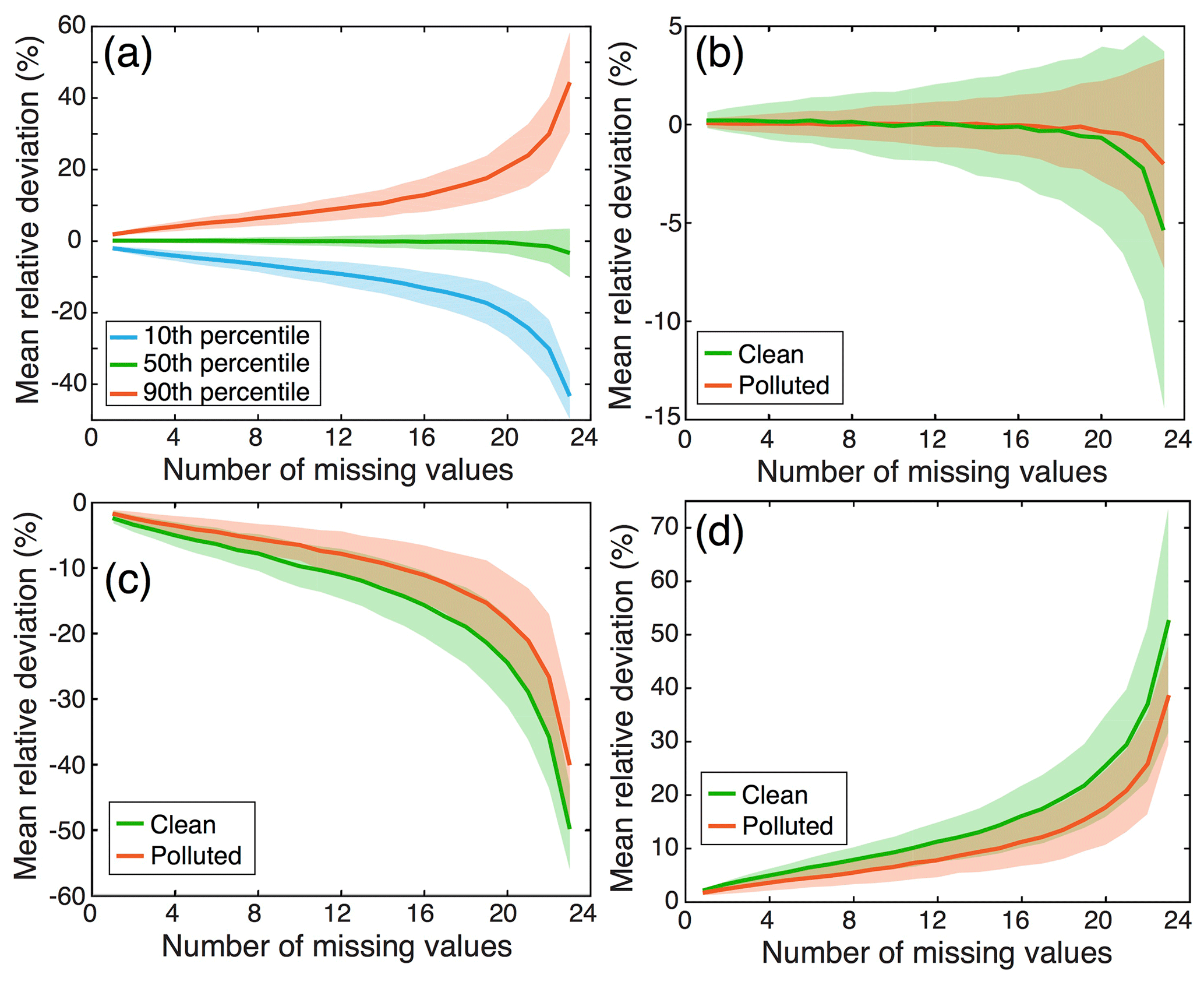
Figure 4 Impacts of the number of missing values on daily averages of PM_2.5. Mean relative deviations were calculated between PM_2.5 daily averages estimated from 1000 hourly PM_2.5 records with a given number of missing values and the original ones without missing values. (a) Deviations at different percentiles in all-sky conditions; (b) deviations at the 50th percentile under different pollution scenarios; (c) same as (b) but for the 10th percentile; (d) same as (b) but for the 90th percentile. Thick lines represent mean deviations, while shaded regions are uncertainties of 1 standard deviation from the mean.

4.2.3 Performance of the DCCEOF method

Cross-validation experiments were first conducted at two monitoring stations to evaluate the efficacy of the suggested DCCEOF method in reconstructing the diurnal cycle of PM_2.5 from the discrete neighborhood field. Specifically, gap-free PM_2.5 records on 3 distinct days with different pollution levels were first extracted randomly at each station, and then six valid observations in each 24 h record were treated as missing values. Subsequently, the DCCEOF method was applied to reconstruct the diurnal cycle of PM_2.5 for each specific case. Figure 6 compares the reconstructed diurnal cycles of PM_2.5 with their actual PM_2.5 concentrations. The results indicate that the reconstructed diurnal cycles of PM_2.5 have a good fit with their actual observations, thus confirming the effectiveness of the DCCEOF method in reconstructing the diurnal variation pattern of PM_2.5 from the discrete neighborhood field. In particular, the DCCEOF method also succeeded in restoring the missing PM_2.5 information even at the inflection times, e.g., the peak value in Fig. 6c and the minimum value in Fig. 6e, which are hard to recover by statistical interpolation approaches. Nonetheless, compared with actual PM_2.5 observations, the reconstructed diurnal cycle of PM_2.5 is still unable to totally restore all types of local variations (e.g., PM_2.5 observations between 07:00 and 11:00 shown in Fig. 6f). This is consistent with our initial understanding that PM_2.5 concentrations vary substantially in space and time, whereas the reconstructed diurnal cycle of PM_2.5 is derived from a limited number of leading EOF modes, and hence it only captures the dominant variation pattern of PM_2.5 in the neighborhood field while some local variations could thus be ignored. In spite of this potential defect, the suggested DCCEOF method still exhibits promising accuracy in restoring the local diurnal cycle of PM_2.5 even from a discrete neighborhood field.

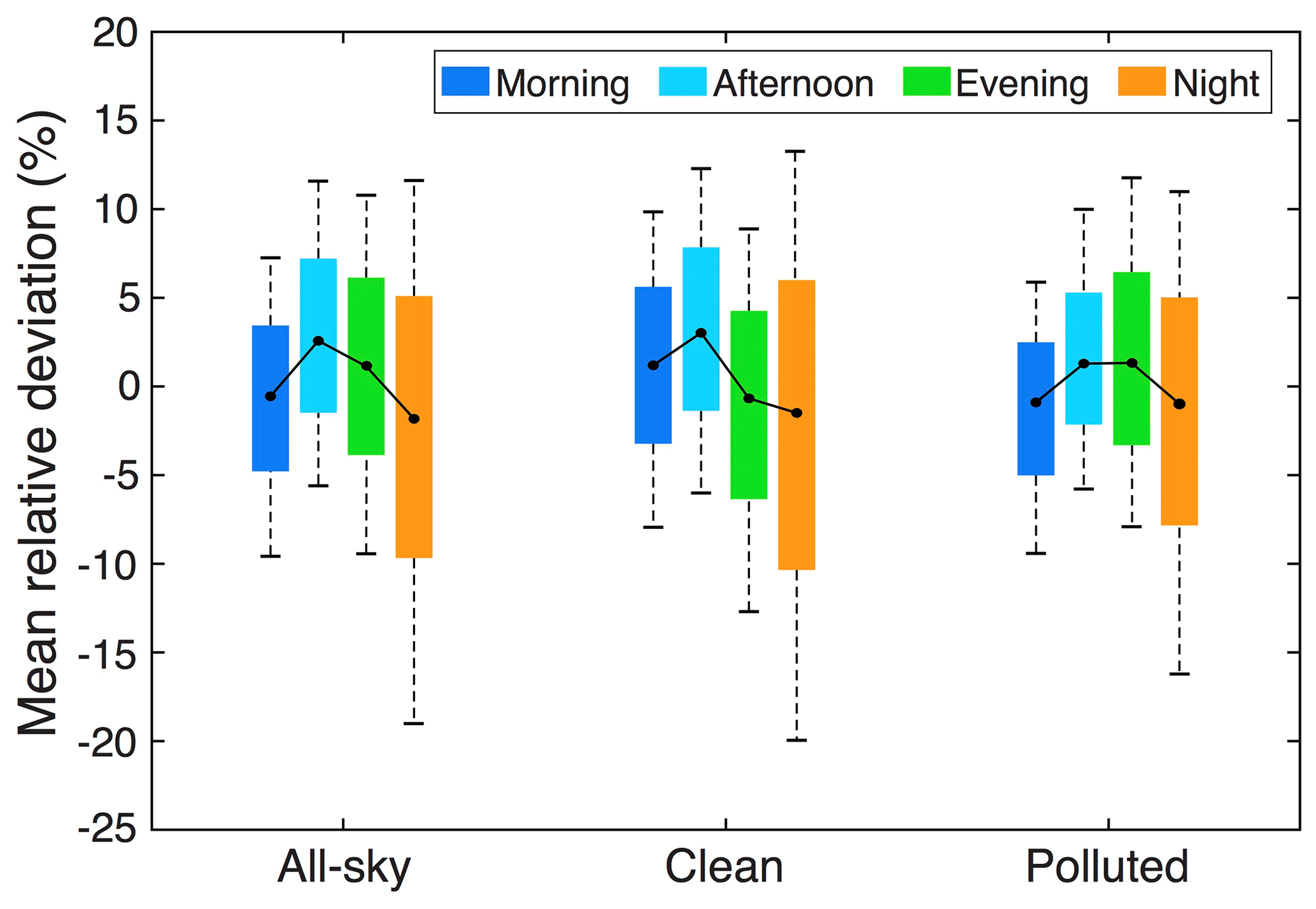
Figure 5 Impacts of diurnal phases of missing values on PM_2.5 daily averages. Hourly PM_2.5 values in the morning (07:00–11:00 CST), afternoon (12:00–16:00 CST), evening (17:00–21:00 CST), and night (22:00–06:00 CST) were removed from the original hourly PM_2.5 time series throughout the day to resemble missing values. On each box, the black dots represent medians of mean relative deviations, while the bottom and top edges of the box indicate the 25th and 75th percentiles, respectively, and the bottom and top whiskers extend to the 10th and 90th percentiles, respectively.

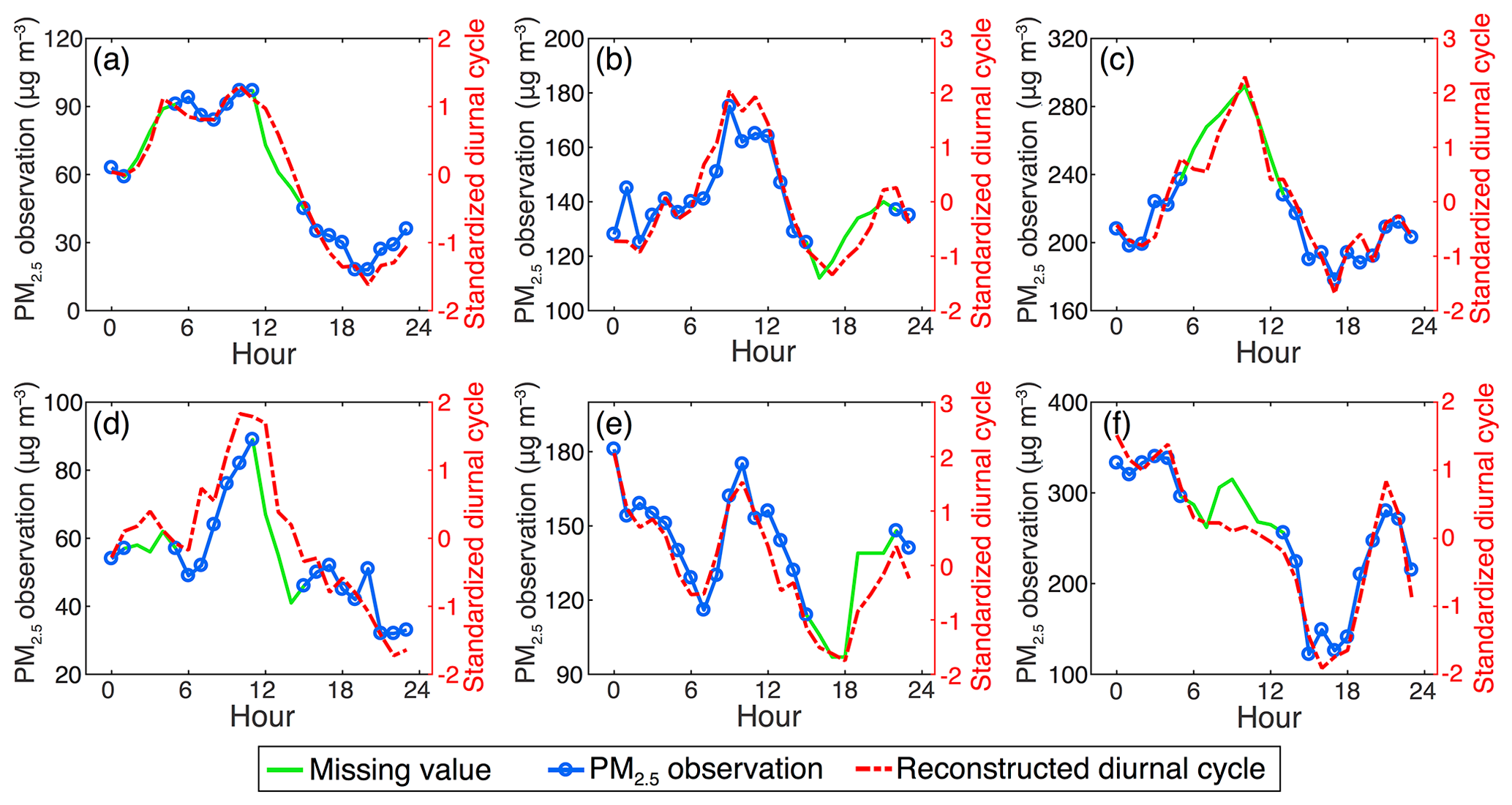
Figure 6 Comparisons of reconstructed diurnal cycles of PM_2.5 with their actual concentrations at distinct pollution levels. For each trial, six valid PM_2.5 observations were selected to simulate gapped PM_2.5 time series prior to the diurnal cycle reconstruction for a given day. Note that the number of neighboring stations differs between these two cases (58 for a–c and 16 for d–f).

To better assess the performance of the DCCEOF method, we retrieved the hourly PM_2.5 observations at one monitoring station in Beijing during the time period of 1 to 7 August 2014, and then some valid observations were retained and then treated as missing values for the subsequent gap-filling practices. Both the DCCEOF method and a spline interpolation approach were used to practically restore the retained PM_2.5 observations. The comparison results shown in Fig. 7 indicate higher accuracy of the DCCEOF method than the spline interpolation approach in restoring those retained PM_2.5 observations, especially for those at the inflection times at which spline interpolation failed to predict with good accuracy (e.g., peak values on 3 August). However, both methods failed in predicting the minimum values on 2 August. After checking the original data record, we found that the local variation in PM_2.5 at this station differed largely from all neighboring stations at that time. For such situations, the suggested DCCEOF method also fails to properly predict the missing values given large differences in diurnal variation patterns in space and time.

Figure 8 presents a more general evaluation of the prediction accuracy of the suggested DCCEOF method, which compares the predicted values with the retained observations at distinct pollution levels. As indicated, there is a good fit between the predicted values and the actual observations, with a correlation coefficient of 0.82 on clean days (Fig. 8a) and 0.95 during polluted episodes (Fig. 8b), respectively. This is in line with our expectation as higher prediction accuracy would be reached by the DCCEOF method in filling data gaps on polluted days given the smaller variability in PM_2.5 concentrations. This effect can also be evidenced by spread scatters shown in Fig. 8a, which in turn reveal the large spatiotemporal heterogeneity of PM_2.5 concentrations during clean scenarios.

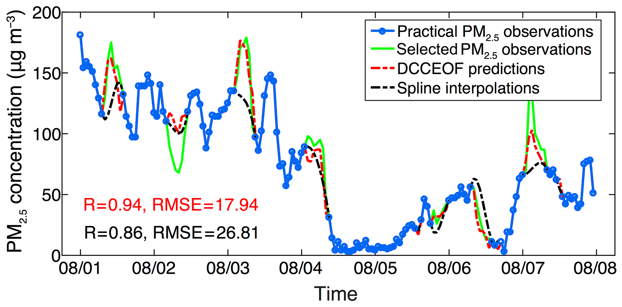
Figure 7 Comparison of predicted hourly PM_2.5 concentration values between the suggested DCCEOF method and spline interpolation at the Wanshou Temple station in Beijing during the period of 1 to 7 August 2014 (time is given as MM/DD on the x axis). The green line shows the practical PM_2.5 observations that were selected to simulate data gaps, while their original values were retained for cross validation.

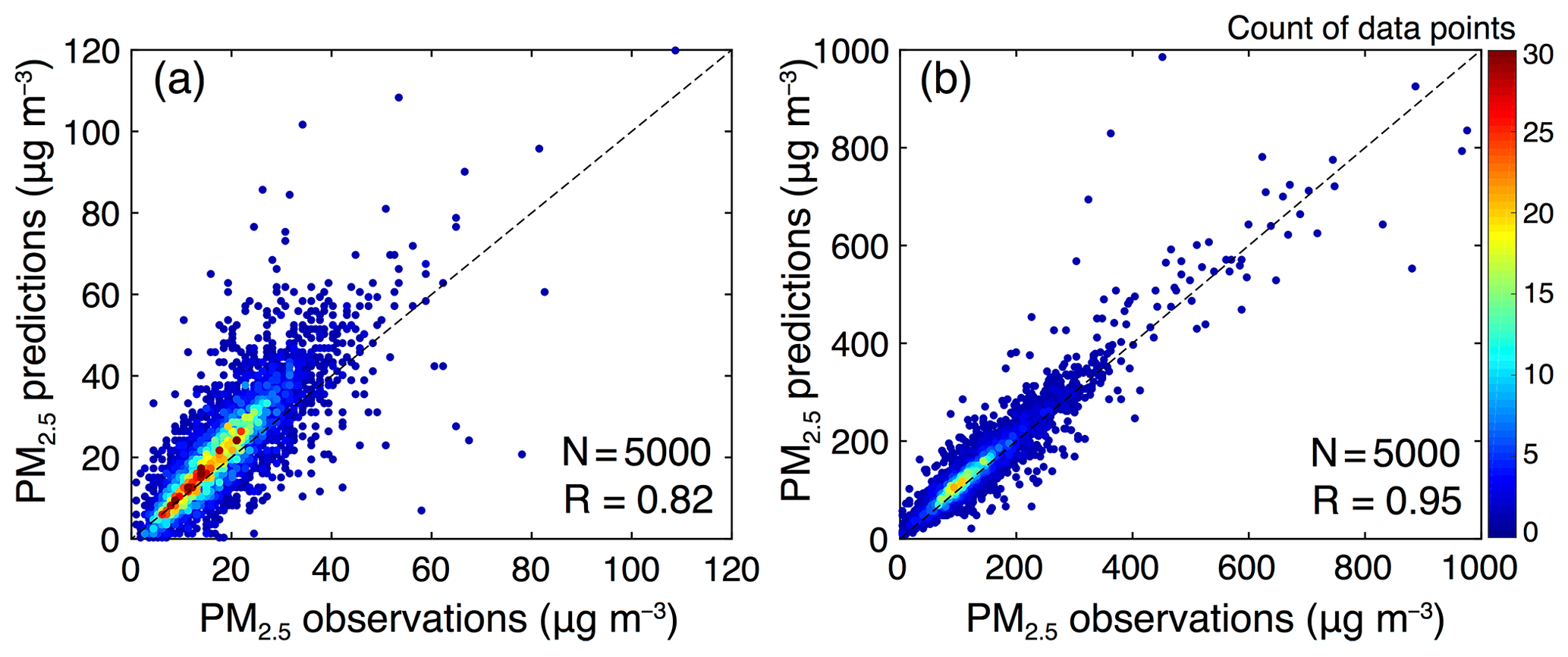
Figure 8 Comparisons of PM_2.5 observations with the reconstructed data values during clean (a) and polluted (b) phases. For each scenario, the results were derived from 1000 d of gap-free PM_2.5 observations with five valid values being randomly retained from 24 h of observations on each sampled date for cross validation.

Given the inherent principle of utilizing discrete neighborhood fields in space and time to reconstruct the local diurnal cycle of PM_2.5 for the subsequent missing-value prediction, the performance of the DCCEOF method could be impacted by the number of missing values and the total number of neighboring stations. To examine the possible dependence of prediction accuracy on these two factors, sensitivity experiments were also conducted. Figure 9a shows the response of prediction accuracy (in terms of the correlation coefficient) of the DCCEOF method to the varying number of missing values in each sampled 24 h PM_2.5 time series. It clearly shows that the prediction accuracy generally decreases with the increase in the number of missing values. This effect can be ascribed to the fact that the target PM_2.5 time series is also applied as a critical constraint for the screening of similar PM_2.5 observations in space and time to construct the neighborhood field for the reconstruction of the local diurnal cycle of PM_2.5. As a consequence, more missingness would make the constructed neighborhood field prone to larger uncertainties due to less information for the selection of relevant time series of PM_2.5, which in turn undermines the overall accuracy of the final predictions.

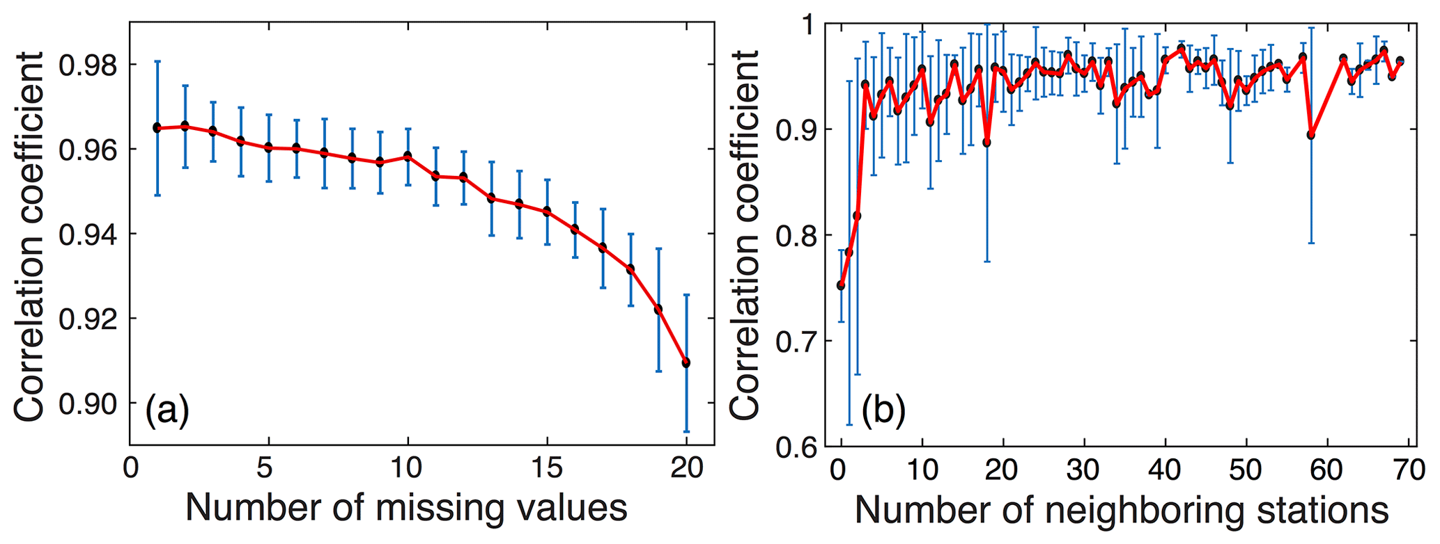
Figure 9 Impacts of the number of missing values present in hourly PM_2.5 records for every 24 h (a) and the total number of neighboring stations within 100 km (b) on the performance of the proposed gap-filling method. The error bars denote 1 standard deviation of each value from the mean on each side.

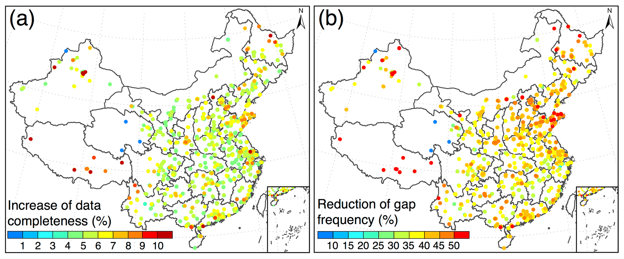
Figure 10 Benefits of the DCCEOF method to our retrieved in situ hourly PM_2.5 records at each individual monitoring station. (a) Improvement of data completeness ratio and (b) reduction of the percentage of days with missingness.

Figure 9b shows the influence of the total number of neighboring stations on the prediction accuracy at the target station. The total number of neighboring stations within a radius of 100 km of the target station was first calculated, and then sensitivity experiments were performed for each specific number. Specifically, 10 stations were randomly selected for each given number, and then 20 d of gap-free PM_2.5 observations were sampled at each individual station. For each gap-free PM_2.5 observation within 24 h, six values were retained and then treated as gaps for cross validation while the DCCEOF method was finally applied to restore these values. It is indicative that the DCCEOF method would have high prediction accuracy with an adequate number of neighboring stations, as three neighboring stations suffice to yield promising prediction accuracy (Fig. 9b). On the other hand, large biases could be introduced into the final predictions with a limited number of neighboring stations (< 3) due to the lack of sufficient prior information from neighbors to reconstruct the diurnal cycle of PM_2.5. Nevertheless, good accuracy can still be guaranteed even in the absence of prior spatial information (that is, no neighboring station within 100 km), which in turn corroborates the beneficial effect of the inclusion of temporal neighborhood in gap filling. Although the prediction accuracy improves with the increase in the number of neighboring stations, the gains in accuracy are not significant at stations with more than three neighboring stations. This is because we only use the similar observations rather than all available observations within 100 km to reconstruct the diurnal cycle of PM_2.5; otherwise, irrelevant observations would distort the reconstructed diurnal variation pattern and in turn the final predictions. Nevertheless, the increase in the number of neighboring stations would reduce the uncertainties in the final predictions, which is evidenced by smaller standard deviations of correlation coefficients for those with more neighboring stations (Fig. 9b). Moreover, the diurnal cycle reconstructed from the neighborhood field in space is more accurate than that using PM_2.5 observations from near-term days, which is evidenced by smaller correlation values with limited neighboring stations. Such an effect is also in line with our recent results when comparing the beneficial effects of spatial and temporal neighboring terms in advancing gridded PM_2.5 concentration mapping (Bai et al., 2019c).

Figure 10 shows the benefits of the DCCEOF method to our retrieved in situ hourly PM_2.5 concentration record at each individual monitoring station in terms of the improvement of the data completeness ratio as well as the reduction of gap frequency. After applying the DCCEOF method, the data completeness ratio of hourly PM_2.5 concentration records in China has been improved by approximately 5 % on average nationwide, with the overall data completeness ratio increasing from 89.2 % to 94.3 % (Fig. 10a). Despite the small magnitude of improvement to the data completeness ratio, the occurrence frequency of missingness has been significantly reduced, with the averaged frequency of days with missingness declining from 42.6 % to 5.7 % nationwide (Fig. 10b). In general, the gap-filled PM_2.5 record is temporally more complete given fewer data gaps, and this data set can thus be used as a promising data source for PM_2.5-related studies in the future.

4.3 Discussion

Compared with conventional interpolation approaches, the suggested DCCEOF method has better accuracy in predicting missing values for the data gaps that emerged in hourly PM_2.5 time series given the principle of accounting for the local diurnal variation pattern of PM_2.5 concentration. Specifically, the site-specific diurnal cycle of PM_2.5 was reconstructed from the discrete spatial and temporal neighborhood using EOF and was then used as a reference to predict missing values. Such a scheme enabled DCCEOF to capture the local variation pattern of PM_2.5 with good accuracy in regions with dense neighboring stations (e.g., eastern China) and fewer temporal dynamics of PM_2.5. In contrast, relatively poor accuracy could be attained in the western part of the country given the lack of adequate neighboring information due to the sparse monitoring stations therein. In such contexts, the performance of DCCEOF could be further improved using a general diurnal variation pattern of PM_2.5 that is firstly determined though a typical classification. However, such an endeavor needs us to have clear prior information on diurnal variability in PM_2.5 in space and time. On the other hand, the diurnal variation pattern of other relevant factors that are highly related to PM_2.5 variations, e.g., meteorological factors such as mixing layer height, might be also applied to advance the reconstruction of the local diurnal cycle of PM_2.5.

Although the DCCEOF method has a promising accuracy in filling data gaps present in hourly PM_2.5 concentration time series, the current method only works for days with at least several valid observations. In other words, the DCCEOF method is incapable of restoring values for days with all 24 h of data missing. This is because the remnant valid observations within 24 h are used as a critical constraint not only to convolve with other neighboring observations in space and time to identify similar observations but also to determine the data magnitude of predicted values for missingness. Moreover, the severity of data gaps in the initial neighborhood field is also associated with the final prediction accuracy because significant data gaps in the neighborhood field could introduce large bias to the reconstructed local diurnal variation pattern. In such contexts, the aforementioned proxy information such as the diurnal variation pattern of meteorological conditions could be applied as a good complement.

5 Conclusions

A novel yet practical gap-filling method termed DCCEOF was introduced in this study to cope with annoying data gaps in geophysical time series, particularly those time series with significant diurnal variability. Compared with the conventional interpolation methods, the suggested DCCEOF method is self-consistent, physically meaningful, and more accurate, given that the local diurnal variation pattern of the monitoring target is accounted for in missing-value restorations. Such an endeavor enables the DCCEOF method to predict missing values even at inflection times, like daily peaks or minima that conventional methods always fail to predict properly, with promising accuracy.

A practical application of the DCCEOF method to our retrieved in situ hourly PM_2.5 concentration record reveals a good prediction accuracy of the DCCEOF method in restoring PM_2.5 missingness. The method performs even better at predicting missing values during polluted phases than it does on clean days given the smaller variations in PM_2.5 concentration in space and time. Further sensitivity experiments suggest that the overall accuracy of the DCCEOF method would slightly decrease (from 0.96 to 0.9) with an increase in the amount of missingness in daily 24 h PM_2.5 observations. This effect is associated with larger uncertainties in the reconstruction of local PM_2.5 neighborhood fields since valid observations are required to convolve with other observations to pinpoint observations with similar variation patterns. Also, an adequate number of neighboring stations in space is essential to the final prediction accuracy of missing-value restoration. The experimental results suggest that three neighboring stations within 100 km of the target station would yield a promising prediction accuracy, and the more neighboring stations there are, the fewer the uncertainties in the final predicted values.

In addition, we also assessed the severity of data gaps in our retrieved China in situ hourly PM_2.5 concentration records. In general, the missingness ratio was less than 10 % over most stations across China, while data gaps occurred more frequently at 06:00 and 12:00 CST than during other times. After gap filling, the data completeness ratio of the China in situ hourly PM_2.5 concentration record was improved to 94.3 %, while the frequency of days with missingness was markedly reduced from 42.6 % to 5.7 %. The gap-filled hourly PM_2.5 concentration record can thus be used as a promising data source for better PM_2.5 concentration mapping and exposure assessment.

Overall, the DCCEOF method developed here provides a realistic and promising way to deal with missingness that emerges in hourly PM_2.5 concentration records which oftentimes exhibit significant diurnal variation patterns. Given its self-consistent nature, the suggested DCCEOF method can be easily applied to PM_2.5 data sets measured in other regions and other geophysical records with similar barriers. A more general comparison of this method with many other conventional gap-filling methods will be conducted in the future to further examine the performance and accuracy of the DCCEOF method in handling various types of data gaps.