the Creative Commons Attribution 4.0 License.
the Creative Commons Attribution 4.0 License.
 | 13 Mar 2020
Aerosol and cloud top height information of Envisat MIPAS measurements
Sabine Griessbach
Lars Hoffmann
Reinhold Spang
Peggy Achtert
Marc von Hobe
Nina Mateshvili
Rolf Müller
Martin Riese
Christian Rolf
Patric Seifert
Jean-Paul Vernier
Infrared limb emission instruments have a long history in measuring clouds and aerosol. In particular, the Michelson Interferometer for Passive Atmospheric Sounding (MIPAS) instrument aboard ESA's Envisat provides 10 years of altitude-resolved global measurements. Previous studies found systematic overestimations and underestimations of cloud top heights for cirrus and polar stratospheric clouds. To assess the cloud top height information and to characterise its uncertainty for the MIPAS instrument we performed simulations for ice clouds, volcanic ash, and sulfate aerosol. From the simulation results we found that in addition to the known effects of the field-of-view that can lead to a cloud top height overestimation, and broken cloud conditions that can lead to underestimation, the cloud extinction also plays an important role. While for optically thick clouds the possible cloud top height overestimation for MIPAS reaches up to 1.6 km due to the field-of-view, for optically thin clouds and aerosol the systematic underestimation reaches 5.1 km. For the detection sensitivity and the degree of underestimation of the MIPAS measurements, the cloud layer thickness also plays a role; 1 km thick clouds are detectable down to extinctions of km−1 and 6 km thick clouds are detectable down to extinctions of km−1, where the largest underestimations of the cloud top height occur for the optically thinnest clouds with a vertical extent of 6 km. The relation between extinction coefficient, cloud top height estimate, and layer thickness is confirmed by a comparison of MIPAS cloud top heights of the volcanic sulfate aerosol from the Nabro eruption in 2011 with space- and ground-based lidar measurements and twilight measurements between June 2011 and February 2012. For plumes up to 2 months old, where the extinction was between and km−1 and the layer thickness mostly below 4 km, we found for MIPAS an average underestimation of 1.1 km. In the aged plume with extinctions down to km−1 and layer thicknesses of up to 9.5 km, the underestimation was higher, reaching up to 7.2 km. The dependency of the cloud top height overestimations or underestimations on the extinction coefficient can explain seemingly contradictory results of previous studies. In spite of the relatively large uncertainty range of the cloud top height, the comparison of the detection sensitivity towards sulfate aerosol between MIPAS and a suite of widely used UV/VIS limb and IR nadir satellite aerosol measurements shows that MIPAS provides complementary information in terms of detection sensitivity.
- Article
(11388 KB) - Full-text XML
- BibTeX
- EndNote


Stratospheric aerosol is known for its impact on radiation and climate (e.g. Crutzen, 2006; Tilmes et al., 2009; Solomon et al., 2011; Santer et al., 2014), atmospheric dynamics (e.g. Wegmann et al., 2014; Diallo et al., 2017), and chemistry (e.g. Tilmes et al., 2008; Wegner et al., 2012; Solomon et al., 2016). Aerosol in the upper troposphere is also of relevance to the Earth's radiation budget (Ridley et al., 2014). The study by Ridley et al. (2014) shows that aerosol in the upper troposphere and lower stratosphere (UTLS) can contribute significantly to the Earth's radiation budget and that the altitude information is important for estimating the radiative impact. Moreover, the available global long-term observations of stratospheric aerosol have a measurement gap in the UTLS at mid and high latitudes (Ridley et al., 2014). This measurement gap has two reasons. First, global long-term measurements are provided by UV/VIS limb instruments (e.g. solar occultation and solar-scattering measurements) that do not measure during night and, hence, miss the entire polar night. Second, as the discrimination between aerosol and thin ice is rather complicated in the UTLS region (Kent et al., 2003), many stratospheric aerosol products terminate at around 15 km and therefore miss part of the lower stratosphere (Ridley et al., 2014). Further, at mid and high latitudes many air traffic corridors are located in the UTLS, and in the case of volcanic eruptions volcanic material can pose a severe danger to air traffic (Casadevall, 1994; Guffanti et al., 2010). Hence, continuous global altitude-resolved aerosol measurements are desirable.
In particular, volcanic eruptions have a significant impact on the stratospheric aerosol load (Kremser et al., 2016). In the tropics even moderate eruptions with a Volcanic Explosivity Index (VEI) of 4 and smaller that only reach the tropopause region contribute to the stratospheric aerosol layer (Vernier et al., 2011). Aside from direct injections alternative transport pathways of aerosol into the tropical stratosphere are still discussed (Bourassa et al., 2012b; Vernier et al., 2013; Fromm et al., 2013; Fairlie et al., 2014; Fromm et al., 2014). Recently it was shown that extra-tropical volcanic eruptions can also contribute to the tropical stratospheric aerosol layer (Schmidt et al., 2010; Diallo et al., 2017; Wu et al., 2017; Günther et al., 2018) and the corresponding transport pathways were uncovered (Wu et al., 2017). However, in order to distinguish between eruptions with plumes restricted to the troposphere and eruptions with stratosphere-reaching plumes and to study the transport pathways in the UTLS, region global measurements with reliable information on the injection heights and aerosol altitudes are required.
Global altitude-resolved measurements of stratospheric and upper tropospheric aerosol are provided by space-based limb measurements and active lidar measurements, e.g. Cloud-Aerosol Lidar with Orthogonal Polarization (CALIOP, Vernier et al., 2011). The limb measurements comprise the solar occultation, e.g. Stratospheric Aerosol and Gas Experiments II, Halogen Occultation Experiment, Polar Ozone and Aerosol Measurement (SAGE, HALOE, POAM, respectively, Randall et al., 2001), Atmospheric Chemistry Experiment Fourier Transform Spectrometer (ACE-FTS), ACE imager (Doeringer et al., 2012; Vanhellemont et al., 2008, respectively), the stellar occultation, e.g. Global Ozone Monitoring by Occultation of Stars (GOMOS, Robert et al., 2016), the solar scattering, e.g. Optical Spectrograph and InfraRed Imager System (OSIRIS, Bourassa et al., 2012a), and the infrared limb emission, e.g. Cryogenic Limb Array Etalon Spectrometer (CLAES, Bauman et al., 2003) and Envisat Michelson Interferometer for Passive Atmospheric Sounding (MIPAS, Griessbach et al., 2016; Günther et al., 2018) measurement techniques.
(Winker et al., 2009)(Prata et al., 2017)(Winker et al., 2009)(Vernier et al., 2009)(Vanhellemont et al., 2010; Sofieva et al., 2013; Robert et al., 2016; Vanhellemont et al., 2016)Vanhellemont et al., 2016(Bertaux et al., 2010; Kyrölä et al., 2010)(Tamminen et al., 2010)(Ackerman, 1997)(Fischer et al., 2008; Höpfner et al., 2009)Sembhi et al. (2012)(Griessbach et al., 2016)(Rieger et al., 2015)(Rieger et al., 2014)Sofieva et al. (2013)Fromm et al. (2014)(Wang et al., 1995; Thomason et al., 1997; Antuña et al., 2002; Thomason et al., 2008)(Thomason and Vernier, 2013)Table 1Overview of relevant instrument characteristics for global aerosol measurements. The minimum detection sensitivity is given for the listed wavelength. The maximum sensitivity indicates the point when the measurements run into saturation, i.e. the top of thicker clouds is always detectable. In the comments column the references are also given.
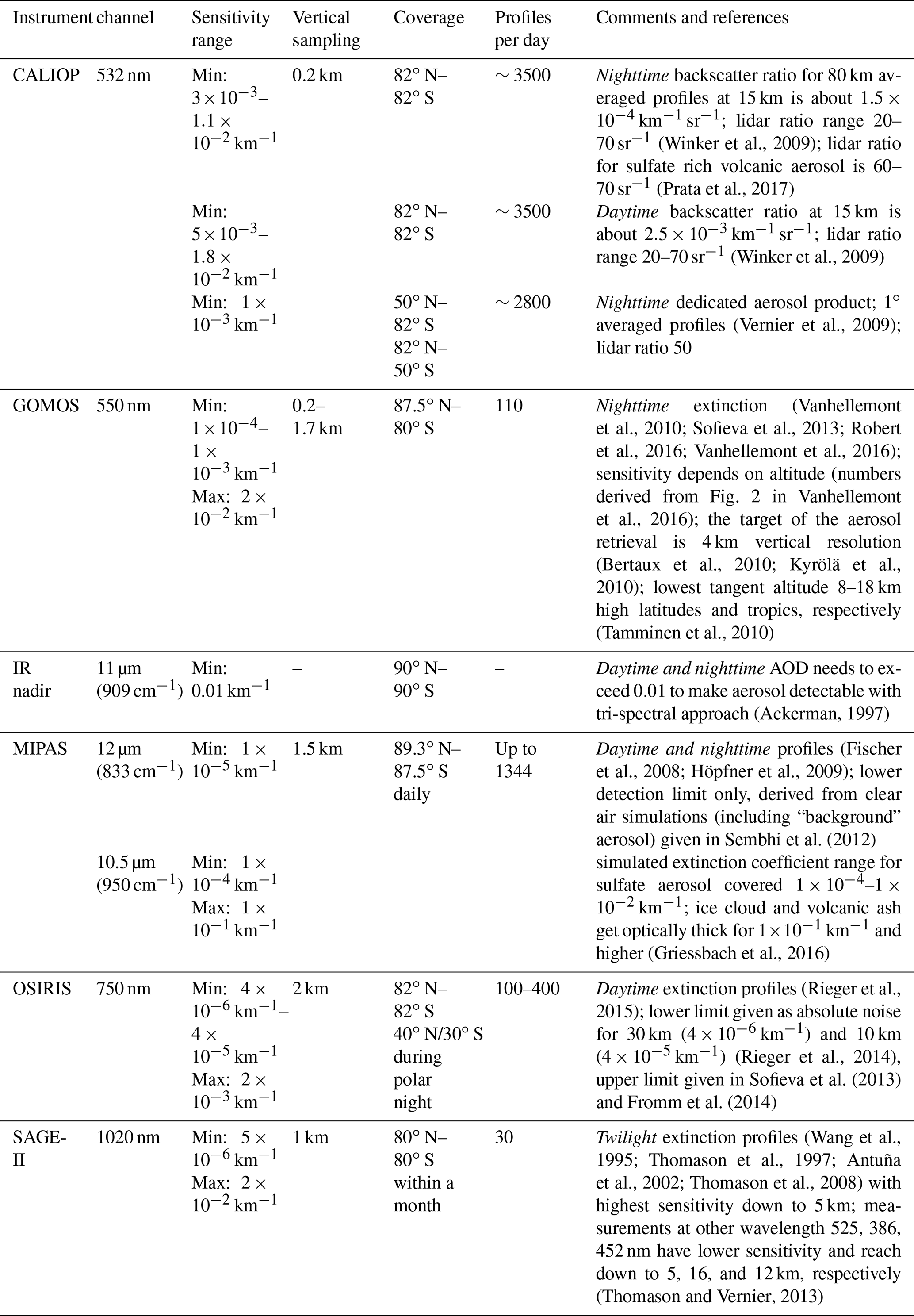
Table 1 summarises the relevant measurement characteristics of selected instruments representing common measurement techniques. In spite of the near-global coverage most instruments have significant temporal and spatial measurement gaps that make their data more suited to studying long-term changes and to developing climatologies than following individual aerosol plumes and identifying distinct sources. For example, GOMOS provides dedicated aerosol measurements during nighttime but misses the daytime hemisphere including the polar summer region. CALIOP provides daytime and nighttime aerosol measurements, yet the nighttime measurements have a significantly higher sensitivity towards aerosol than the daytime measurements. In contrast, OSIRIS measures only at daytime and SAGE-II measured during sunrise and sunset. Figures showing the differences in the latitudinal coverage and the sampling frequencies of typical solar and stellar occultation, solar scattering, and infrared limb emission measurements can be found in Sofieva et al. (2013, Fig. 2) and Robert et al. (2016, Fig. 2).
Infrared nadir measurements provide an excellent global coverage at daytime and nighttime but have a significantly lower sensitivity towards aerosol than limb measurements due to their measurement geometry. It has been shown that enhanced volcanic sulfate aerosol can also be detected with infrared nadir measurements (Ackerman, 1997; Clarisse et al., 2013). However, in general, the altitude retrieval competes with the concentration and radius retrieval (Clarisse et al., 2010), and e.g. dust aerosol altitudes retrieved from Atmospheric Infrared Sounder (AIRS) measurements indicate the altitude where half the aerosol optical depth (AOD) of the entire layer is reached (Peyridieu et al., 2010).
Lidar measurements (ground based, air-borne, or space based) are considered to provide the best altitude information. Studies comparing e.g. SAGE II with lidar measurements smoothed the vertically higher resolved lidar data to SAGE II vertical resolution (e.g. Antuña et al., 2002) and extinction profiles of e.g. GOMOS and OSIRIS have been validated against SAGE II and SAGE III (e.g. Robert et al., 2016; Bourassa et al., 2012a, respectively). Studies assessing or validating the aerosol and cloud altitude information from limb remote sensing measurements are rare. Only Kent et al. (1997) investigated the accuracy and potential error sources of SAGE II cloud heights. Using two flights of airborne lidar cloud measurements they simulated the signal SAGE II would receive for these clouds. For the 41 simulated scenarios Kent et al. (1997) found an overestimation of the cloud top height in a single case and an underestimation by 1 to 5 km in 17 cases (39 %). The underestimation was attributed to patchy clouds, where the cloud was located along the ray path but not at the tangent point. For CALIOP a very good agreement of cloud and aerosol altitudes was found compared with in situ balloon and lidar measurements and ground-based lidar measurements (Vernier et al., 2009; Mioche et al., 2010; Kim et al., 2011). Compared with ground-based lidar measurements, Kim et al. (2008) found that the CALIOP cloud top and base heights generally agree within 0.1 km.
Due to MIPAS' large field-of-view smoothing the signal over an altitude range of about 3 km, several studies investigated the viability of MIPAS cloud top heights. For polar stratospheric clouds (PSCs) Höpfner et al. (2009) found that MIPAS systematically underestimates the cloud top height by about 0.3 (at 15 km) and up to 2.6 km (at 27 km) compared to CALIOP. The underestimation of cloud top height shows a clear altitude dependence where the large underestimation at high altitudes was attributed to broken cloud conditions. Castelli et al. (2011) investigated the effect of broken cloud conditions on MIPAS cloud top heights and confirmed the underestimation effect for 1-D cloud detection methods, but showed that a 2-D retrieval can lead to significant improvements if the cloud was sampled by consecutive MIPAS profile scans. For cirrus clouds Spang et al. (2012) quantified MIPAS' underestimation up to 2.5 km compared to SAGE II. In contrast, MIPAS was found to overestimate cirrus cloud top heights by usually less than 2 km compared to Geoscience Laser Altimeter System (GLAS) measurements during the Space Shuttle Mission (Spang et al., 2012). Sembhi et al. (2012) also reported an overestimation of about 1 km compared to CALIOP and of about 0.75 km compared to HIRDLS in a comparison of 3-monthly means of aerosol and cloud top heights. This overestimation was attributed to MIPAS' field-of-view, where optically dense clouds below the tangent point, but within the field-of-view, affect the measured radiances. Based on simulations of idealised clouds Hurley et al. (2009) proposed an operational retrieval framework that is supposed to retrieve cloud top heights with an error below 0.5 km.
As the MIPAS measurements have the potential to fill gaps in the measurements of UTLS aerosol and clouds, the goal of this study is to assess the cloud top altitudes derived from the MIPAS aerosol and cloud index detection methods (Spang et al., 2004; Sembhi et al., 2012; Griessbach et al., 2016), to reconcile the contradictory results of previous MIPAS cloud top height studies, and to add a comparison for sulfate aerosol, which has not been investigated explicitly before. This study is based on MIPAS radiance simulations for aerosol and ice clouds and a comparison between MIPAS and CALIPSO, ground-based lidar, and twilight measurements of the Nabro volcanic sulfate aerosol between June 2011 and January 2012. The instruments and aerosol data products for MIPAS, CALIOP, the ground-based lidars, and the twilight measurements are introduced in Sect. 2. In Sect. 3 the simulated aerosol and cloud scenarios are described and the derived top heights are analysed and assessed. The dedicated comparison of the top heights for the Nabro sulfate aerosol is presented in Sect. 4. A discussion of the simulation results and the comparison of the cloud top heights for the volcanic sulfate aerosol follow in Sect. 5. The conclusions are given in Sect. 6.
2.1 MIPAS
MIPAS was an infrared limb sounder that was mounted on ESA's Envisat and operated from June 2002 to April 2012. It measured up to 1344 vertical profiles per day (14.4 orbits with 96 profiles) at daytime and nighttime covering the latitudes between 89.4∘ N and 87.3∘ S. The high-resolution emission spectra in the thermal infrared (685–2410 cm−1) comprise altitudes between 6 and 68 km from July 2002 to March 2004 and 7 to 72 km from January 2005 to April 2012 in MIPAS' nominal mode (Fischer et al., 2008). The nominal mode was changed due to a malfunction of the instrument in 2004. From 2002 to 2004 the vertical sampling was 3 km and in 2005 the vertical sampling was decreased to 1.5 km below 21 km altitude. In addition, the formerly homogeneous measurement geometry was changed so that the lower measurement heights approximately follow the tropopause; i.e. in the tropics MIPAS sampled down to 10 km and in the polar regions down to 7 km. The MIPAS engineering tangent altitudes, which are corrected for refraction, have a negative offset of about 300 to 500 m compared to retrieved altitudes in the UTLS height range (Kleinert et al., 2018). The vertical width of the field-of-view of MIPAS is about 3 km. For retrieval of MIPAS measurements, the field-of-view is often assumed to be trapezoidal with edge lengths of 2.8 and 4 km (Ridolfi et al., 2000; Hurley et al., 2009). The horizontal field-of-view, which is perpendicular to the line-of-sight, is 30 km (Fischer et al., 2008). As Envisat flew in a Sun-synchronous orbit, MIPAS measured at daytime and nighttime with a mean local solar time of around 22:00 for the ascending node and 10:00 for the descending node.
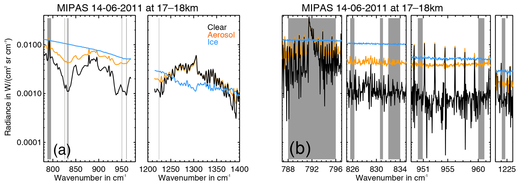
Figure 1Representative MIPAS spectra for clear air, ice cloud, and aerosol measured on 14 June 2011 between 17 and 18 km altitude. (a) MIPAS band A and B spectra smoothed to 1 cm−1 spectral resolution. (b) High-resolution MIPAS spectra only in the window regions used for aerosol or cloud detection and discrimination. The grey background indicates the window regions.
To derive aerosol we used the MIPAS band A (685–970 cm−1) and band B (1215–1500 cm−1) level 1b data set processed with the instrument processing facility (IPF) processor version 7.11 that provides calibrated and geolocated radiances. A method to detect aerosol in the UTLS and filter out ice clouds has been introduced by Griessbach et al. (2016). This aerosol detection methods relies on two steps. First, for improved aerosol and cloud detection the aerosol cloud index (ACI) with values smaller than 7 is used. The ACI is the maximum of the cloud index and the aerosol index that are the colour ratios between the CO2 band at 788.25–796.25 cm−1 and two atmospheric window regions at 832.31–834.37 and 960.00–961.00 cm−1, respectively. In the second step the discrimination between aerosol and ice clouds is performed using threshold functions for brightness temperature difference correlations between the following windows: 860.6–831.1, 960.0–961.0, and 1224.1–1224.7 cm−1. Each spectrum of a profile is evaluated with this two-step method and is identified as either clear air, aerosol, or ice cloud with the corresponding tangent height as altitude information. In order to ensure that the MIPAS aerosol measurements used in our study only comprise sulfate aerosol, first the aerosol and cloud detection was performed, the ice clouds were filtered out as described above, and finally the volcanic ash detection method using two additional windows at 825.6–826.3 and 950.1–950.9 cm−1 (Griessbach et al., 2014), which was also found to be sensitive to mineral dust and wildfire aerosol, was applied to filter out other non-sulfate UTLS aerosol types. The characteristic spectral signatures of clear air, an ice cloud, and a sulfate aerosol layer are illustrated in Fig. 1 with selected measured MIPAS spectra, showing the broadband signatures in bands A and B with a 1 cm−1 smoothed spectrum (Fig. 1a) and the relevant window regions with the original high spectral resolution (Fig. 1b).
2.2 Space-based lidar CALIOP
CALIOP is an active lidar instrument onboard the Cloud-Aerosol Lidar and Infrared Pathfinder Satellite Observation (CALIPSO) that has flown in the A-Train constellation since 2006 (Winker et al., 2009). The satellite is in a Sun-synchronous polar orbit with the local Equator-crossing time of the ascending node at about 13:30 and of the descending node at about 01:30 that allows for measurements at daytime and nighttime between 82∘ N and 82∘ S (Winker et al., 2009). CALIOP is a near-nadir-viewing two-wavelength polarisation-sensitive lidar (Winker et al., 2009). The best signal-to-noise ratio is provided by the nighttime measurements at 532 nm (Vernier et al., 2009).
Focusing on aerosol measurements in this study, a dedicated aerosol product providing the highest sensitivity is used: after applying a cloud mask that is based on the ratio between the perpendicular and total backscatter signal at 532 nm, CALIOP nighttime profiles were averaged horizontally over 1∘ latitude and vertically over 200 m (Vernier et al., 2009). Each day reflections of 1.7 million laser shots are acquired (Winker et al., 2009). Assuming 111 km averaging, a 40 009 km circumference of the Earth from pole to pole, and 14.55 orbits per day, this results in about 2800 independent nighttime profiles. The optimised aerosol measurements cover the winter hemisphere up to 82∘ and the summer hemisphere up to 50∘ and have a further gap due to the South Atlantic Anomaly (Vernier et al., 2009). For the comparison of the measurements of the Nabro aerosol in boreal summer we used data between 0 and 50∘ N and between 12 and 20 km. The Nabro aerosol was visible in individual CALIOP profiles between 15 June and 11 August 2011. To convert the backscatter signal to the extinction coefficient we used a constant lidar ratio (aerosol extinction to backscatter ratio) of 50 sr as Sawamura et al. (2012) mostly used this ratio and reported one measured lidar ratio of 48 sr at 532 nm for the Nabro sulfate aerosol.
2.3 Ground-based lidars
2.3.1 Leipzig, Germany
In Leipzig (51.34∘ N 12.37∘ E), regular lidar measurements are performed with the Multiwavelength Atmospheric Raman lidar for Temperature, Humidity, and Aerosol profiling (MARTHA) (Mattis et al., 2002) in the framework of the European Aerosol Research Lidar Network (EARLINET, Pappalardo et al., 2014) three times each week, i.e. Monday afternoon and Monday and Thursday after sunset, when weather conditions allowed (i.e. absence of precipitation and low clouds). The light source is a Nd:YAG laser that generates laser pulses at 355, 532, and 1064 nm wavelengths with a repetition rate of 30 Hz. The backscattered radiation is collected by a 0.8 m Cassegrain telescope. The aerosol backscatter coefficient can be determined at 355, 532, and 1064 nm and the aerosol extinction coefficient at 355 and 532 nm is derived by means of the Raman-lidar method (Ansmann et al., 1992) (not available for all layers). The system detects the component of light cross-polarised to the plane of polarisation of the outgoing beam at 532 nm. MARTHA observations have been used previously for the statistical characterisation of free-tropospheric aerosol layers (Mattis et al., 2008), volcanic aerosol layers (Mattis et al., 2010), and the characterisation of polar stratospheric clouds (Jumelet et al., 2008).
The aerosol signal was derived from backscatter signals under cloud-free conditions only by averaging the data between 27 min and 6 h (on average 2:09 h). From the averaged signal the layer top and bottom altitude were derived from the gradient of the averaged signal profile following Mattis et al. (2008). After the cloud boundary determination the optical depth was calculated at 532 nm wavelength from the Raman-derived aerosol backscatter coefficient for layers observed during nighttime (Ansmann et al., 1992). For each nighttime layer we also computed the average extinction at 532 nm. The conversion from backscatter coefficient to extinction coefficient requires the assumption of a backscatter-to-extinction (lidar) ratio. Although for Leipzig measurements of stratospheric aerosol usually a lidar ratio of 30 sr is used, which was derived from measurements within the first 2 years after the eruption of the Pinatubo volcano (Mattis et al., 2008), here we used a lidar ratio of 50 sr to make the average layer extinctions comparable to CALIOP. The choice of a higher lidar ratio is further supported by Sawamura et al. (2012), who derived a lidar ratio of 48 sr from measurements of Nabro aerosol, and Prata et al. (2017), who derived lidar ratios around 60±15 sr in the first 2 weeks after the sulfur-rich eruptions of Kasatochi and Sarychev. The errors in the layer boundary heights and particle backscatter coefficients are approximately 300 m and 20 %, respectively, due to the low signal-to-noise ratio and small signal gradient produced by the sulfate layers of the Nabro volcano. The Nabro aerosol was measured over Leipzig between 5 July 2011 and 10 February 2012 on 47 d (59 lidar profiles). These profiles were checked for other aerosol sources, such as Grimsvötn sulfate aerosol (Tesche et al., 2011) and wildfires, that were removed from the data for the altitude comparison.
2.3.2 Jülich, Germany
A ground-based cloud lidar was operated by the Jülich research centre located in the western part of Germany (50.92∘ N, 6.36∘E; 91 m a.s.l.). The lidar system is a commercial lidar instrument (Leosphere, ALS 450) that operates at a wavelength of 355 nm with a pulse energy of 16 mJ, a pulse duration of 4 ns, and a frequency of 20 Hz (Rolf et al., 2012). The parallel and perpendicular polarised backscattered light is measured by two detectors to determine the depolarisation. The receiver telescope has a diameter of 15 cm with a full-angle field-of-view of around 1.5 mrad. The covered altitude range is from 0.5 to 19 km with a vertical resolution of around 30 m depending on atmospheric conditions.
The lidar is usually operated at times where, potentially, cirrus clouds are present. Thus, the operation is irregular in time and only complete cloud-free sequences were selected for this study. The Nabro aerosol was measured over Jülich between 15 July and 12 December 2011 on 7 d (11 lidar profiles). The backscatter profiles used in this study were vertically smoothed with a window length of 360 m to increase the signal-to-noise ratio above 12 km. Sawamura et al. (2012) reported lidar ratios of 45 and 55±1 sr at 355 nm for the Nabro aerosol. As in both cases the lidar ratio at 355 nm was 7 sr larger than at 532 nm for the same sample, we used a lidar ratio of 55 sr. The aerosol layer top and bottom altitudes were derived based on a comparison of the signal to the signal-to-noise ratio. Additionally, we checked that the thermal tropopause derived from ERA-Interim reanalyses is below the Nabro aerosol layer.
2.3.3 Esrange, Sweden
The Department of Meteorology of Stockholm University operates a lidar at Esrange (67.89∘ N, 21.10∘ E) near the Swedish city of Kiruna (Blum and Fricke, 2005; Achtert et al., 2013). The Esrange lidar uses a pulsed Nd:YAG solid-state laser as a light source. A detection range gate of 1 µs results in a vertical resolution of 150 m. The backscattered light at 532 nm is detected in two orthogonal planes of polarisation. The molecular fraction of the received signal was determined from the vibrational Raman signal.
Measurements with the Esrange lidar were only conducted during campaigns. The lidar was in operation between 4 and 25 January 2012, measuring on 6, 9, 13, 14, 19, 20, and 25 January. Within this study the parallel and perpendicular backscatter ratios, the particle backscatter coefficient, and the linear particle depolarisation ratio were used. The extinction coefficients presented here have been obtained using the Esrange lidar's rotational Raman channels (Achtert et al., 2013) that do not require any lidar ratio. Measurements with these channels have also been used to derive the temperature profile from which the tropopause height has been inferred.
2.4 Twilight measurements
Spectral photometric measurements of the twilight sky brightness are performed in Tbilisi, Georgia (41.72∘ N, 44.78∘ E), on a regular basis every clear day at solar zenith angle range 90–96∘ (Mateshvili et al., 2005). From 2009 a CCD camera with a grating spectrograph is used to record a time series of spectral images between 685 and 800 nm. The images are averaged over the wavelength interval 777.5 to 782.5 nm and the corresponding acquisition time moments are converted to solar zenith angles. The thus obtained dependencies of the monochromatic brightness of the twilight sky on the solar zenith angles are used to retrieve aerosol extinction vertical profiles. The aerosol extinction profiles at 780 nm and the corresponding errors were retrieved in the UTLS (Mateshvili et al., 2013).
The post-Nabro aerosol profiles were acquired 11 times between 14 July and 3 August 2011 from the Tbilisi observational site. In this study we used the derived extinction profiles at 780 nm (12820.5 cm−1) and the corresponding errors that are given on a 1 km grid. The actual vertical resolution of the retrieved aerosol extinction profiles were estimated from the half-widths of the maximums of the averaging kernels at the respective altitudes up to 1.5–2 km for the Nabro aerosol layer (Mateshvili et al., 2013).
These twilight data are the only ground-based data set that has an overlap with the CALIOP measurements. As it relies on an entirely different technique than the lidar measurements, it further allows for checking of the consistency between the various aerosol layer top height definitions.
3.1 Simulation setup
The radiative transfer model used for the MIPAS simulations is the Jülich Rapid Spectral Simulation Code (JURASSIC) (Hoffmann et al., 2008). The fast radiative transfer and retrieval model was used to calculate spectrally averaged radiances on MIPAS' spectral grid based on pre-calculated emissivity look-up tables and the emissivity growth approximation (EGA) (Weinreb and Neuendorffer, 1973; Gordley and Russell, 1981). JURASSIC was extended to account for single scattering on aerosol and cloud particles where the optical properties were calculated using Mie theory (Griessbach et al., 2013).
For the simulation of IR limb emission spectra in the presence of clouds and aerosol we followed the setup described in Griessbach et al. (2014) with some modifications. We placed three 1 km thick homogeneous sulfate aerosol, ice cloud, and volcanic ash layers at 9–10, 13–14, and 17–18 km and one 6 km thick sulfate aerosol layer at 10–16 km altitude for the four representative atmospheric states of a polar winter, polar summer, midlatitude, and equatorial atmosphere (Remedios et al., 2007). Although MIPAS samples the UTLS at 1.5 km in the vertical, the pencil beam simulations were performed on a 0.5 km grid and interpolated to a 0.1 km grid after applying MIPAS' trapezoidal field-of-view, in order to account for the fact that real clouds are located at any vertical distance to the sampling altitudes. The simulations cover the tangent height range between 8.5 and 20 km.
For the particle shape we assumed spherical particles, which is realistic for the liquid sulfate aerosol and an approximation for ice and volcanic ash. The IR refractive indices were taken from Hummel et al. (1988) for sulfate aerosol (75 % sulfuric acid solution), Warren and Brandt (2008) for ice, and Pollack et al. (1973) for basalt as a representative for volcanic ash. Each particle type has its individual realistic particle size and extinction coefficient ranges as reported by in situ measurements (see Griessbach et al., 2014, for a discussion of the ranges). For sulfate aerosol we considered median radii between 0.01 and 1.5 µm of a lognormal size distribution with a width of 1.6 (which corresponds to effective radii between 0.02 and 2.6 µm) and selected the particle number concentration such that it resulted in extinction coefficients between and km−1 in half an order of magnitude steps at 950 cm−1. For ice clouds the median radius range was 0.3 to 96 µm and the extinction coefficient range to 1 km−1, and for volcanic ash the median radii ranged from 0.1 to 5 µm and the extinction coefficients included to km−1.
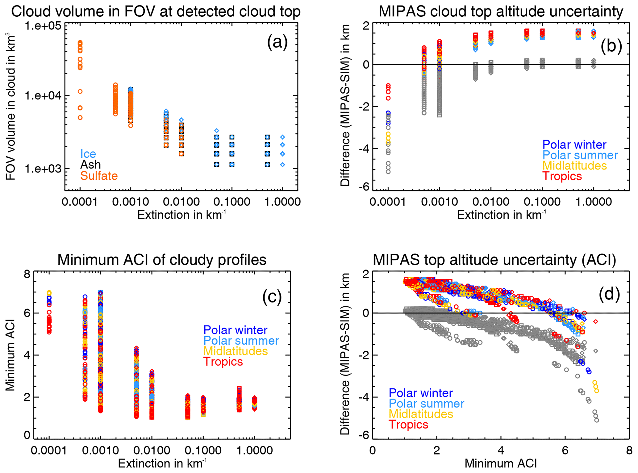
Figure 2Characterisation of the cloud top height derived from simulations. (a) Volume of the field-of-view filled with cloud at the detected cloud top height as a function of extinction. The colours indicate the particle type: orange – sulfate aerosol, blue – ice, and black – volcanic ash. (b) Top height difference (detected–real top height) as a function of extinction. (c) Minimum ACI value within a cloudy profile as a function of extinction coefficient. (d) Top height difference as a function of minimum ACI value within a cloudy profile. In all panels the symbols indicate the particle type: circles – sulfate aerosol, diamonds – ice, and squares – volcanic ash. In panels (b), (c), and (d) the colours indicate the background atmosphere type: red – tropics, orange – midlatitudes, light blue – polar summer, and dark blue – polar winter. In panels (b) and (d) the coloured symbols show the top height uncertainties of all scenarios for the simulated 100 m vertical sampling grid. For the MIPAS vertical sampling of 1.5 km the coloured symbols indicate the upper limit and the grey symbols indicate the lower limit of the top height uncertainty range. Depending on the position of the cloud relative to the tangent altitude, the detected top height may fall anywhere in between. See the text and Table 2 for details.
3.2 Results: MIPAS detection sensitivity and top height uncertainties
To detect aerosol and clouds with MIPAS we used the ACI and considered the cloud top to be the first tangent altitude where the ACI falls below 7 (Griessbach et al., 2016). In the following the term “cloud top height” refers to the top altitude of ice cloud, ash, and sulfate aerosol layers. A comparable sensitivity to the cloud index (CI) method (Spang et al., 2005) using altitude- and latitude-dependent thresholds by Sembhi et al. (2012) was reported in Griessbach et al. (2016) for this method. We found that the 1 km thick aerosol layers are detectable down to an extinction coefficient of km−1, which is in agreement with previous results by Griessbach et al. (2016). In addition, we found that the 6 km thick aerosol layer is in some (but not all) cases detectable down to the extinction coefficient of km−1. This is because the vertically larger layer fills a larger volume of the field-of-view. For each detected cloud top height Fig. 2a shows the cloud-filled field-of-view volume integrated along the line-of-sight as a function of the extinction coefficient. Further, Fig. 2a indicates that the integrated cloudy field-of-view volume at the detected cloud top does not depend on the particle type. This justifies our approach of combining ice cloud, ash, and sulfate aerosol simulations for the characterisation of the cloud top uncertainty. The variability is rather a function of the tangent altitude.
The dependency of the detection sensitivity on the extinction coefficient and the integrated cloudy field-of-view volume also has implications for the detected cloud top height. The fine grid simulation results show that the cloud top height mainly depends on the extinction coefficient: some effect can be seen for the background atmosphere and nearly no effect can be seen for the different particle types (Fig. 2b, coloured symbols). Transferring the fine grid simulation results to the coarser MIPAS vertical sampling, the resulting maximum altitude ranges around the “real” cloud top height are given in Table 2. The potential uppermost detected top height on the MIPAS sampling grid is the same as on the fine grid. The lowermost top height (Fig. 2b, grey symbols) results from the following consideration: if the cloud top is detected at 18 km on the 100 m simulation grid and the MIPAS tangent heights are at 18.1 and 16.6 km (1.5 km vertical sampling), the measured MIPAS cloud top height would be 16.6 km. While the top height of thick clouds can be overestimated by up to 1.6 km due to the field-of-view, the cloud top of clouds with an extinction of km−1 and smaller can be underestimated by up to 5.1 km (for the 6 km thick layer) due to the field-of-view and extinction effect (Table 2). Depending on the position of the cloud relative to the tangent height, the detected top height may fall anywhere in between the ranges given in Table 2.
In practice, when analysing MIPAS measurements the extinction coefficient of any cloud or aerosol layer is unknown unless an extinction retrieval is available. Hence, one cannot judge whether the cloud top height is overestimated or underestimated. The simulated ACI at the cloud top is always close to 7; however, analysing the entire profile provides more information. The cloud layers with an extinction of km−1 or smaller result in profiles with a pronounced local ACI minimum (e.g. see the measured MIPAS profile in Fig. 5), whereas for thicker clouds the ACI profiles run into saturation with ACI values around 2 (Fig. 2c). From Fig. 2d, showing the relation between the minimum ACI of a profile and the height difference, we deduce that for saturated ACI profiles the derived cloud top height overestimates the real cloud top height in most cases. For profiles with a local ACI minimum the cloud top height can be overestimated or underestimated and the minimum ACI can be used as a rough indicator of the likelihood of overestimation or underestimation (Fig. 2d). For minimum ACIs smaller than 3 there is a strong tendency towards overestimation and the possible underestimation is less than 1.5 km. For minimum ACI values larger than 5.5 there is a strong tendency towards underestimation and the overestimation is less than 0.6 km. In general, the smaller the minimum ACI, the more likely an overestimation, and the larger the minimum ACI, the more likely an underestimation of the cloud top height.
Table 2Range of cloud top height uncertainty as a function of the extinction coefficient derived from the simulations. The cloud top is the altitude where ACI <7. The results are given on the 0.1 km fine grid of the simulations and transferred to the 1.5 km vertical sampling of MIPAS. Please see the text for details.
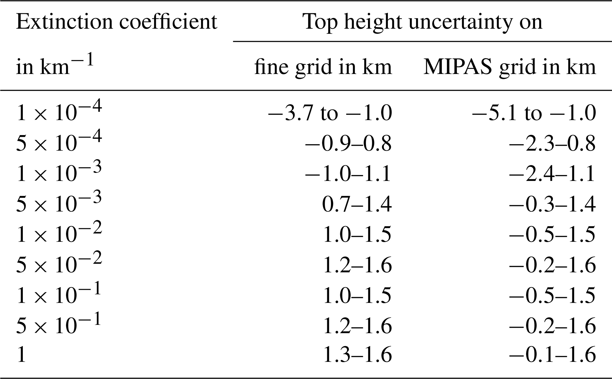
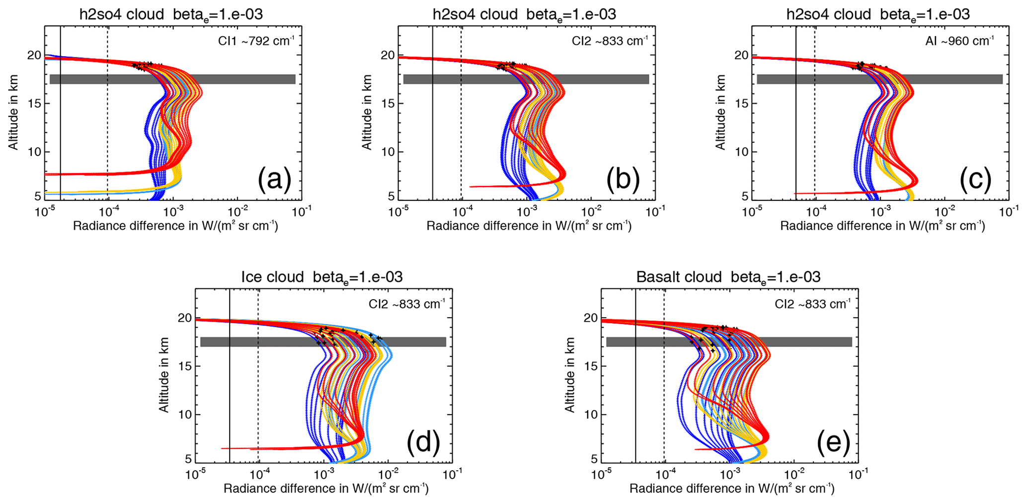
Figure 3Increase in radiance (cloud – clear air simulation) due to different clouds (solid coloured lines) compared to NESR (black solid line), offset accuracy (black dashed line), and scaling accuracy (dotted coloured lines; very close envelopes around solid coloured lines) for sulfate aerosol in (a) the CI window around 792 cm−1 (CI1), (b) the CI window around 833 cm−1 (CI2), and (c) the AI window around 960 cm−1, and (d) for ice (e) and ash. The colours indicate the background atmosphere type: red – tropics, yellow – midlatitudes, light blue – polar summer, and dark blue – polar winter. Each line represents one particle size distribution. The black symbols indicate the detected cloud top altitude using ACI =7.
3.3 Error estimation
The idealised simulations above do not contain any instrument errors. To assess the potential impact of MIPAS instrument errors on the cloud detection using the ACI, we compared the increase in radiance due to aerosol/clouds with the average noise equivalent spectral radiance (NESR) of W m−2 sr−1 cm for the optimised resolution mode, the total scaling accuracy of 2.4 %, and the total offset accuracy of W m−2 sr−1 cm for band A (Kleinert et al., 2018). Although by absolute value the NESR appears to be the largest error, it is reduced by , because we averaged over n=17, 34, and 129 spectral points in the three ACI windows, respectively. The exemplary selected profiles for the three windows in Fig. 3 show that the increase in radiance at cloud top altitude is well above both the NESR and the offset error, while the scaling accuracy results in a very tight envelope around the increase in radiance. From this consideration we deduced that using an ACI value above 7 ensures that no instrument effects are accidentally interpreted as a cloud. Moreover, Fig. 3 shows that the particle size distribution causes a significant spread of the increase in radiance (for ice clouds, sulfate aerosol, and ash with km−1 the spread at cloud top is , , and W m−2 sr−1 cm, respectively), and hence can be considered an important source of variability.
4.1 Nabro eruption
For the comparison with other measurements we focus on the eruption of the Eritrean Nabro volcano that started on 12 June 2011 around 20:32 UTC (Goitom et al., 2015). With an SO2 emission of about 4.5 MT within 15 d (Theys et al., 2013) this eruption released the largest amount of SO2 during the MIPAS measurement period between 2002 and 2012. This eruption is known to have injected few to no ash particles (Theys et al., 2013). The injection reached the UTLS region (Sawamura et al., 2012), where accurate knowledge of the altitude is crucial for scientific conclusions (Bourassa et al., 2012b; Vernier et al., 2013; Fromm et al., 2014).
4.2 Method
The Nabro sulfate aerosol in the UTLS was measured by inherently different measurement techniques that have individual sensitivities with respect to the aerosol layer extinction coefficient, top height, and thickness. Hence, we compared the various definitions of aerosol layer top height and the corresponding aerosol detection sensitivities of the instruments used in this study individually. For the MIPAS measurements we used ACI ≤7, the ice, and ash cloud filter methods (Sect. 2.1) to identify the cloud top height of the Nabro aerosol layers. From the simulation study we already derived that aerosol layers with extinctions down to km−1 are detectable and that the detection height and the corresponding uncertainty range strongly depend on the layer extinction (Sect. 3.2).
Table 3Scaling factors for the extinction coefficient of sulfate aerosol from 948.5 cm−1 (10.5 µm, MIPAS) to the wavelengths used by selected satellite instruments, the ground-based lidar and twilight measurements, and for the MIPAS CI.

To make the MIPAS measurements with their detection limits comparable to the lidar and twilight measurements, we estimated the scaling factors between the wavelengths of the lidar, and twilight measurements and 10.5 µm, the wavelength of the MIPAS simulations (Fig. 4). As the extinction coefficient of sulfate aerosol has a strong dependency on the wavelength (wavenumber) and particle size, we used five measured sulfate aerosol size distributions (PSDs) after the Mt. Pinatubo (Deshler et al., 1992b, a, 1993, four PSDs) and Nabro (Bourassa et al., 2012b, one PSD) eruptions and calculated the corresponding extinction coefficient spectra from 0.2 to 16 µm using Mie calculations and the refractive indices of Hummel et al. (1988) for 75 % sulfuric acid solution. Further, we fitted three representative mono-modal log-normal PSDs to the minimum ( µm), maximum ( µm), and middle extinction ( µm) spectra assuming a distribution width of 1.6 (Fig. 4). The spectra are normalised to 948.5 cm−1 (dashed line) as this is the wavenumber used to set the extinction coefficients for our MIPAS simulations. The scaling factors from 948.5 cm−1 (10.5 µm) to the wavelengths used for the lidar, twilight measurements, and selected satellite instruments introduced in Sect. 1 are given in Table 3 as a range (minimum to maximum) for the measured PSDs and fitted PSDs individually.
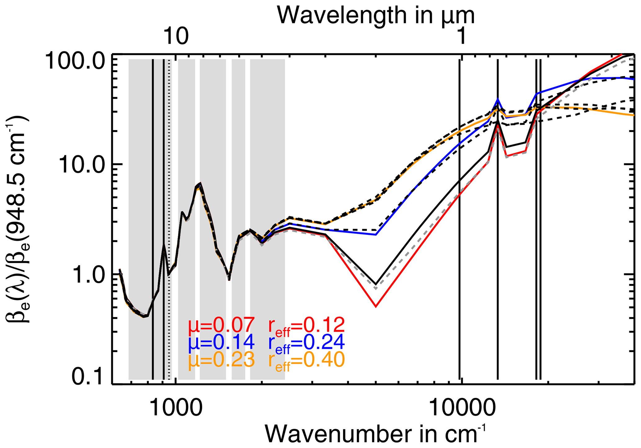
Figure 4Extinction coefficient spectra normalised to 1 at 948.5 cm−1 for modelled sulfate aerosol particle size distributions (coloured lines) and measured size distributions after Pinatubo (black dashed lines; Deshler et al., 1992a, b, 1993, Arctic), Nabro (grey dashed line; Bourassa et al., 2012b, July, Wyoming), and background aerosol at 20 km (black solid line; Deshler et al., 2003, April 1999). The corresponding scaling factors are given in Table 3.
The individual cloud top height definitions of the CALIOP and ground-based measurements used for the comparison are presented in the following Sects. 4.3–4.7 individually as well as the chosen match criteria and the results.
4.3 CALIOP measurements
Most global comparisons between MIPAS and CALIOP were performed on a statistical basis using temporal and regional mean cloud top height values, because ice clouds are highly variable in space and time. Especially in the tropics the match times (about 3:30 h difference in local Equator-crossing time) and match distances between MIPAS and CALIPSO are rather large in terms of cloud-extent scales and formation timescales (e.g. Hurley et al., 2011; Sembhi et al., 2012; Spang et al., 2012, 2015). For PSCs, which persist on longer timescales and have a larger horizontal extent than convective clouds, Höpfner et al. (2009) compared individual profiles of MIPAS and CALIOP measurements. Volcanic sulfate aerosol we consider also sufficiently temporally persistent to allow for a comparison of individual profiles (Kent et al., 1997), but still keep in mind that very fresh plumes can be very localised. We set the temporal match time for the comparison of MIPAS and CALIOP aerosol detections to 6 h, as in Höpfner et al. (2009). As a match radius we selected 500 km, which is the along-track distance between two MIPAS measurements. Given the fact that the longitudinal distance between two subsequent MIPAS (and CALIOP) orbits increases from about 500 km at 80∘ N to 1800 km at 50∘ N, and to 2800 km at the Equator, the choice of 500 km allows for a sufficient number of matches for statistics between 50∘ N and the Equator. The choice of a 500 km match radius for an aerosol measurement comparison is further supported by the match criteria discussed by Antuña et al. (2002) for SAGE II ranging from ±1 to 5∘ in latitude (about 111–555 km) and from ±1 to 25∘ in longitude (about 111–2775 km at the Equator and 72–1800 km at 50∘ N) and their finding that for aged plumes the results did not depend on the match criteria. As CALIOP has a much higher along-track sampling rate than MIPAS (Fig. 7), we calculated the mean extinction profile of all CALIOP profiles within the match radius. In total we found 1190 MIPAS aerosol profiles with a matching CALIOP profile within the first 8 weeks after the Nabro eruption (12 June to 11 August 2011).
For comparison of the cloud top heights, the definition of the cloud top is crucial. While for MIPAS the aerosol detections are defined by the ACI threshold and the cloud top height is the highest tangent altitude where the ACI falls below 7, which is sensitive to extinctions down to km−1 (at 10.5 µm), for the CALIOP extinction profiles we first used a detection sensitivity threshold and second used the extinction gradient to derive the cloud top height.
4.3.1 Results for extinction threshold method
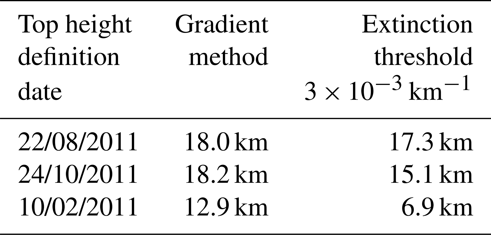
CALIOP's nominal extinction threshold (at 532 nm) is km−1 at 18 km and km−1 at 12 km altitude for nighttime measurements averaged over 80 km horizontally and 60 m vertically and assuming a lidar ratio of 50 sr−1 (Winker et al., 2009). For the aerosol product used in this study the CALIOP data were averaged over 111 km horizontally and 200 m vertically. Hence, the detection limit should be even lower. Figure 5 shows single CALIOP profiles and the corresponding averaged profile for a match with MIPAS. A match may contain between one and nine single CALIOP profiles depending on where the CALIPSO track crosses the match radius. For averaging, only profiles were used where the maximum extinction exceeds the detection sensitivity; i.e. clear air profiles were excluded from averaging. Around 15 km a clear aerosol signal is visible, whereas at altitudes above about 17 km and below about 14 km the signals get rather noisy. For the averaged profile the noisy signal is below km−1 and for the single profiles it is below km−1. This is a further indication that the detection limit of the dedicated CALIOP aerosol product is lower.
Figure 5Nabro sulfate aerosol layer measured by CALIOP and MIPAS. (a) The red line is the averaged lidar profile of the individual lidar profiles within the match range (black lines). The grey dashed line indicates the altitude-variable extinction coefficient threshold of km−1 at 18 km used to estimate the top height of the aerosol layer (Winker et al., 2009). (b) The gradient of the averaged lidar profile, where the cross at the maximum gradient indicates the top height according to the gradient method described by Mattis et al. (2008). (c) MIPAS ACI profile. The dots mark the tangent altitudes, where grey dots indicate clear air, red dots aerosol, and blue dots ice clouds. The black solid line marks the ACI detection threshold of 7.
In order to find the CALIOP detection threshold that provides a comparable sensitivity towards sulfate aerosol to MIPAS, we first scaled the MIPAS detection limit of km−1 to the CALIOP wavelength (532 nm) yielding about 2.5– km−1 (at 18 km) depending on the particle size distribution (see Table 3). This is lower than the detection limit for the standard CALIOP aerosol product of km−1 at 18 km (Winker et al., 2009). However, the detection limit of the aerosol product used in this study was expected to be somewhat lower than the limit for the standard product due to more averaging. To verify that the aerosol product used here has a lower detection limit, we counted the number of matches with CALIOP when moving the altitude-variable detection limit (Fig. 5, dashed line) to lower and larger values. The results are given in Fig. 6 with the extinction coefficient of the altitude-variable detection limit at 18 km on the x axis. In total there are 1190 MIPAS aerosol profiles with a CALIOP match. For extinction thresholds between 1 and km−1 the number of matches is constant at 1153. It decreases by 1 at km−1, by 10 at km−1, and by 70 at km (Fig. 6). From this decrease we deduce that the detection sensitivities of MIPAS and the dedicated CALIOP aerosol product are comparable for extinction thresholds ranging from about 2 to km−1 (at 532 nm). In the following the results for the altitude-variable extinction threshold that is km−1 at 18 km are shown. That this choice is appropriate can be seen in Fig. 7 showing the top heights of MIPAS and CALIOP Nabro aerosol measurements and giving an impression of the data coverage of both measurements within 24 h.
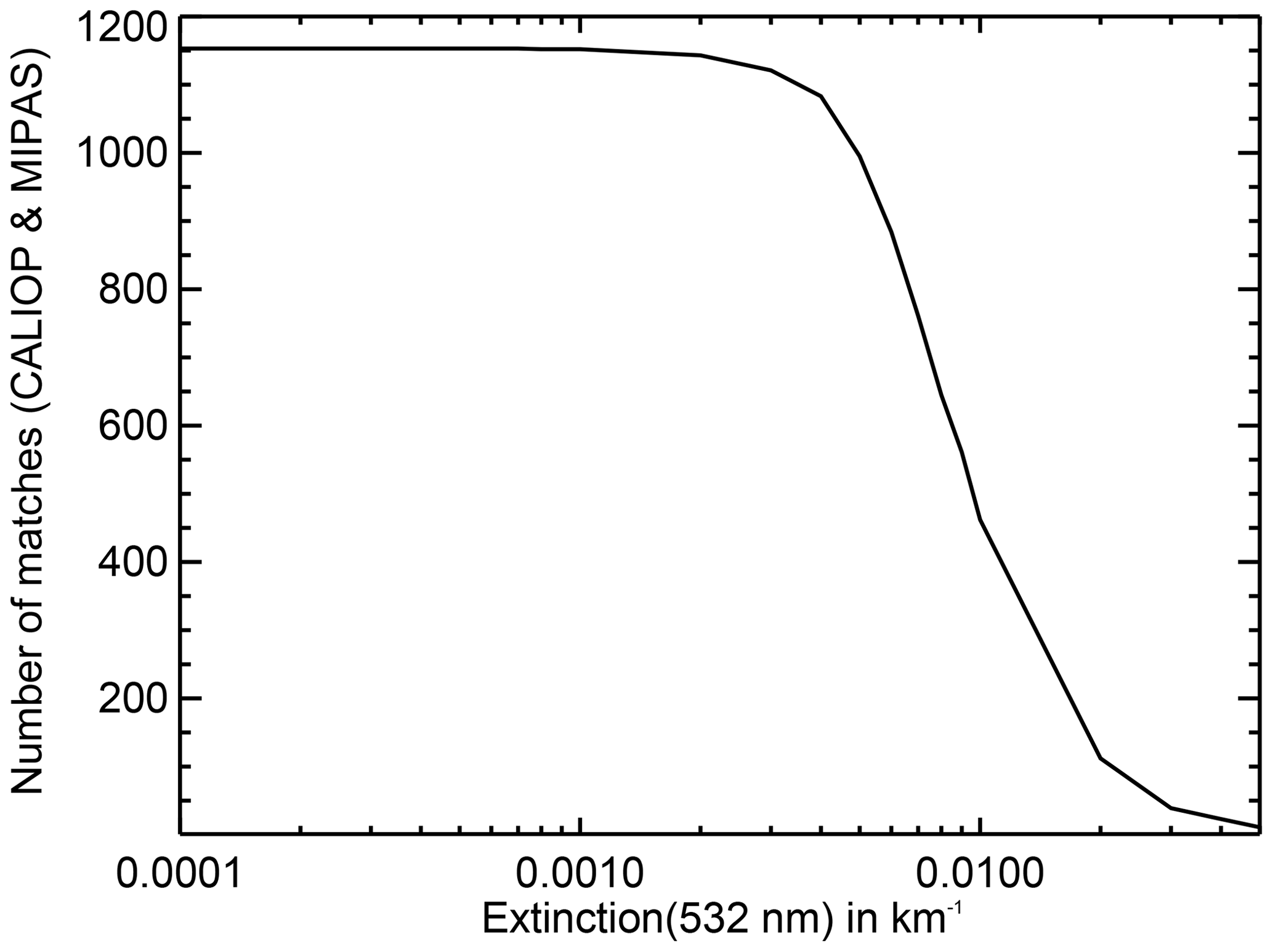
Figure 6Number of matches for MIPAS and CALIOP aerosol detections as a function of the altitude-variable extinction threshold for CALIOP given at 18 km.

Figure 7Sulfate aerosol detected by MIPAS (circles) and CALIOP (squares) (a) 10 d and (b) 48 d after the Nabro eruption. The MIPAS orbit tracks, indicated by grey dashes, reach up to 90∘ N and the CALIOP orbit tracks of available aerosol data are indicated by black dots. The colours indicate the layer top height. For CALIOP aerosol detections an altitude-variable extinction threshold that is km−1 at 18 km was used.
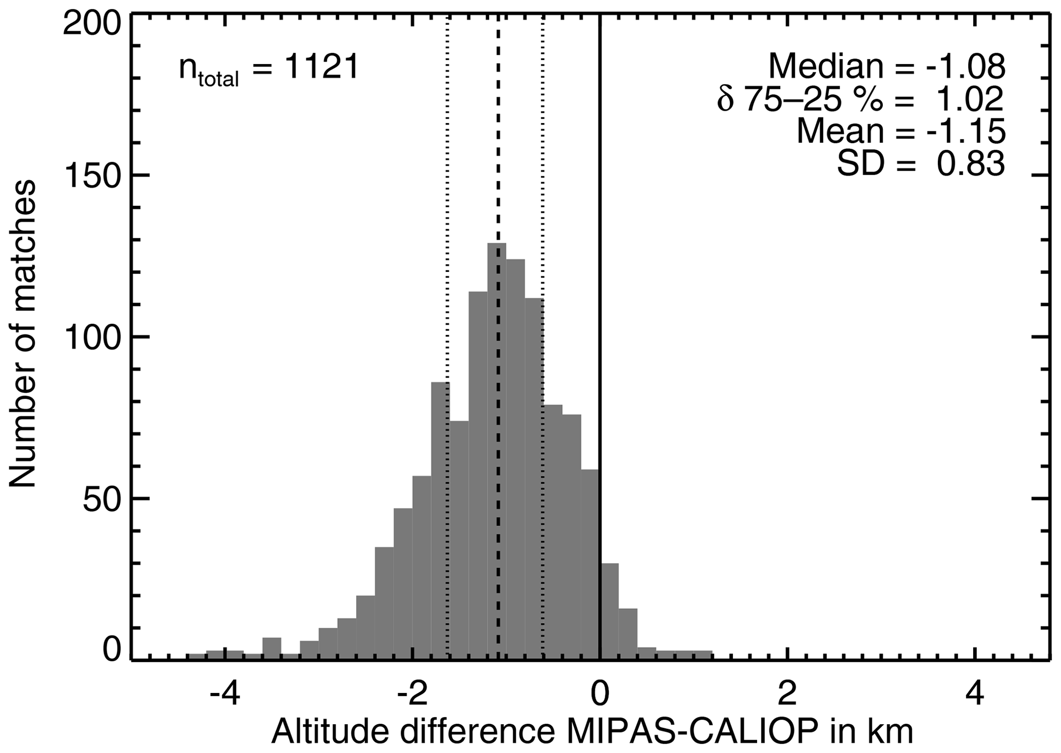
Figure 8Distribution of cloud top height differences (MIPAS–CALIOP) for aerosol measurements of the Nabro sulfate aerosol in June, July, and August 2011. The cloud top height from CALIOP was derived using an altitude-variable extinction threshold that is km−1 at 18 km. The black dashed line indicates the median, the dotted lines are the 25th and 75th percentiles, and the solid line marks the zero difference.
The result of the comparison of the individual MIPAS and CALIOP aerosol profiles is shown in Fig. 8. MIPAS underestimated the cloud top height of the Nabro sulfate aerosol by 1.08 km in median and 1.15 km in mean. In 95 % of all matches the cloud top height was underestimated and in 5 % it was overestimated. Individual differences reached up to 1 km and −5.9 km. In only three cases the overestimation was more than 1 km and in only two cases the underestimation was more than 5 km. This result is in line with the altitude uncertainty range given by the simulation results in Sect. 3, where the overestimation reached up to 1.6 km and the underestimation was up to 5.1 km. In 2.4 % of the matches the underestimation was more than 3 km. The analyses of the correlations between extinction coefficient and altitude difference (Fig. 9a), extinction coefficient and minimum ACI (Fig. 9b), and minimum ACI and altitude difference (Fig. 9c) show that the comparison results mainly fall within the ranges predicted by the simulations (compare with Fig. 2b, d, and c, respectively). Outliers we attributed to potentially bad matches and in the case of the smallest simulated extinction to the rather small set of simulated scenarios. The correlations also show that the Nabro aerosol was thin and not optically thick to MIPAS with ACI values larger than 2.5 (Fig. 9c) and extinctions between and km−1 in the VIS range being equivalent to – km−1 in the IR (10.5 µm).
Table 4Difference between MIPAS and CALIOP cloud top height of the Nabro sulfate aerosol for the extinction coefficient threshold method and the gradient method for a possible set of scaling factors determining the altitude-variable extinction detection threshold, where the threshold value is given at 18 km.
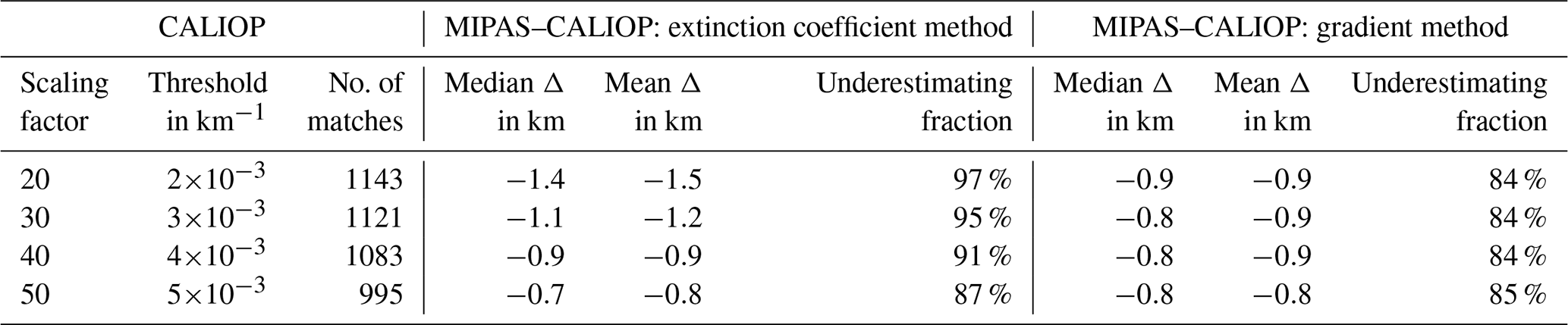
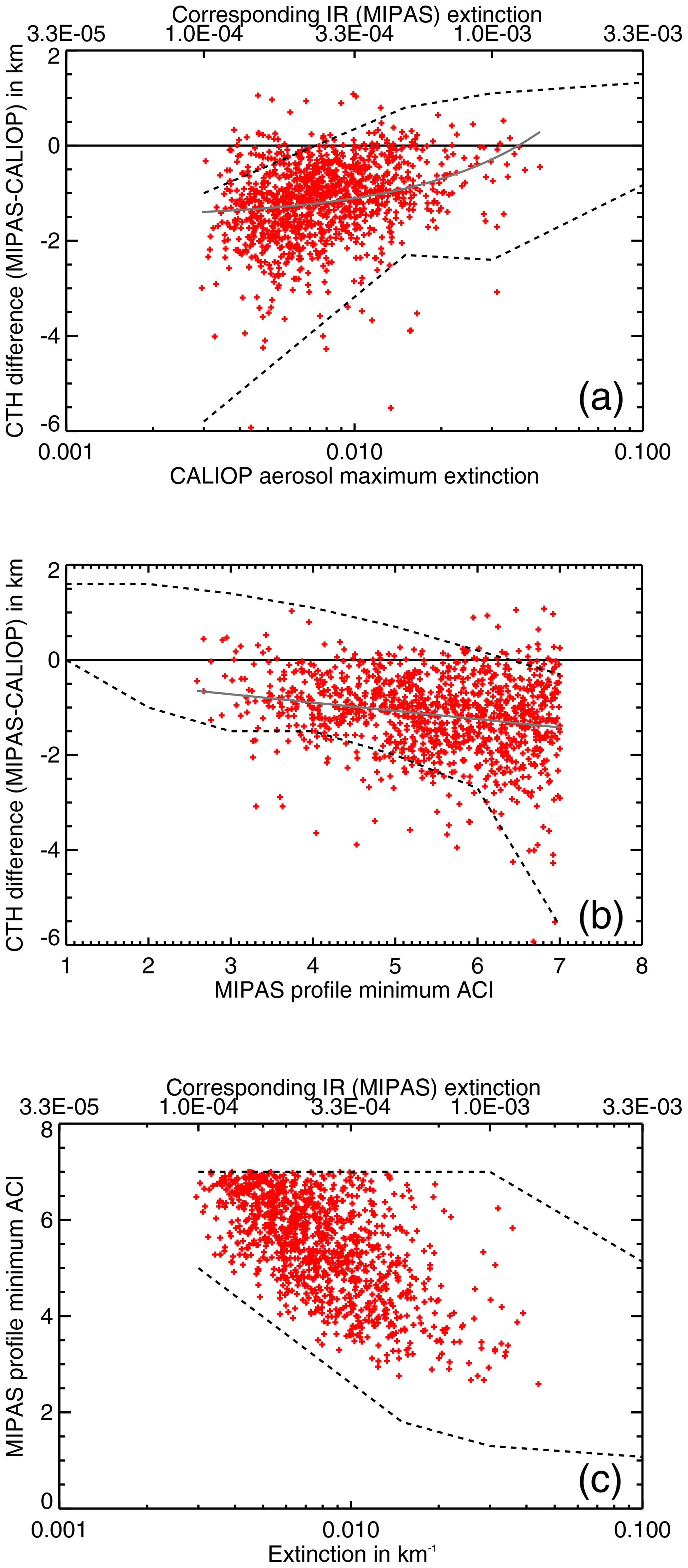
Figure 9Cloud top height differences between MIPAS and CALIOP Nabro aerosol measurements (using a CALIOP extinction threshold of 3 km−1), as a function of (a) CALIOP aerosol layer maximum extinction, and (b) MIPAS minimum ACI. (c) shows the diagnostic relation between CALIOP maximum extinction and MIPAS minimum ACI. The black dashed lines indicate the ranges expected from the simulations (see Fig. 2).
The sensitivity of the analysis to our selected extinction threshold was tested by performing the same analysis with extinction coefficient scaling factors of 20, 40, and 50. With a larger extinction threshold for CALIOP the number of matches decreased and the average underestimation for MIPAS also decreased by about 200 m with each step, as the cloud top height is at a lower point in the aerosol layer. However, for all threshold values the top height was underestimated in 87 %–97 % of all cases (Table 4).
4.3.2 Results for the gradient method
A common method to derive aerosol and cloud layer top and bottom altitudes from ground-based lidar data is the gradient method (Mattis et al., 2008). Different from Mattis et al. (2008), we calculated the extinction gradient between two successive data points in each CALIOP profile and assigned the gradient to the altitude in between (Fig. 5, middle). The maximum of the gradient was used as the indicator for the cloud top height. The advantage of this method is that it is independent of any extinction threshold. The disadvantages, however, are that this method also provides results for noisy clear air profiles and that it misses thinner layers above a thick aerosol layer, because it provides only the overall maximum. To filter out clear air profiles we ran the analyses using extinction thresholds between and km−1 as a pre-filter.
Compared to the CALIOP cloud top heights derived by using extinction coefficient thresholds, the gradient method provides lower top heights in 60.4 % of all matches for a threshold of km−1 and 13.6 % for km−1 and higher top heights in 1.5 % of all matches for a threshold of km−1 and 23.0 % for km−1. The maximum agreement between both methods we found for km−1, where 63.4 % of all cloud top heights agreed within 100 m. From visual inspection of the profiles we found that the gradient method provides lower cloud top heights than the extinction threshold method, because it misses thin aerosol layers above thicker layers, and for smaller extinction thresholds the cloud top height moves up. For larger extinction thresholds thinner layers are also filtered out and, hence, both methods show a better agreement.
As the cloud top height derived by the gradient method does not depend strongly on the extinction threshold chosen as a pre-filter, the median and mean differences between MIPAS and CALIOP cloud top height are relatively constant, ranging from −0.8 to −0.9 km for extinction coefficient thresholds below km−1 (Table 4). This result is comparable with the result using an extinction coefficient threshold of km−1, yet the underestimating fraction is 7 percentage points smaller for the gradient method, although still high at 84 % (Table 4). Since we found that the gradient method, as we implemented it, misses thinner aerosol layers above thick layers, we used the results from the extinction threshold method with a threshold of km−1 in the further course of this study.
Table 5Nabro sulfate aerosol measured by the Leipzig lidar and MIPAS. For the lidar data aerosol layer top, bottom, and mean extinctions (for nighttime profiles) are given. For MIPAS, the number of matching profiles, the mean cloud top height, and the corresponding minimum and maximum top heights are given.

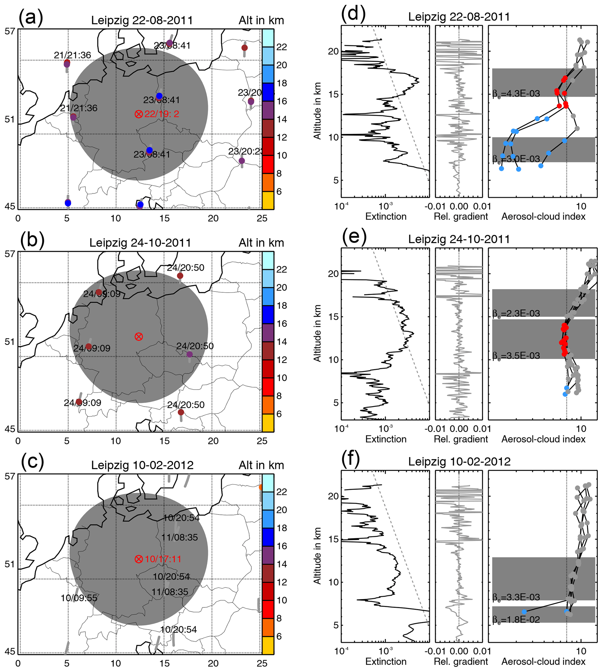
Figure 10Nabro aerosol measured by the Leipzig lidar and MIPAS on (a, d) 22 August 2011, (b, e) 24 October 2011, and (c, f) 10 February 2012. (a, b, c) The maps show the lidar station, lidar measurement time, match radius, MIPAS orbits, MIPAS profile measurement time, and MIPAS cloud top height (colour coded). (d, e, f) Left: Leipzig lidar extinction profile (black line) and the extinction coefficient threshold of km−1 at 18 km (grey dashed line). Middle: the relative extinction gradient (grey line). Right: MIPAS ACI profiles within the match range. The grey dots denote clear air, red dots denote sulfate aerosol, and blue dots denote ice and optically thick clouds. The black dotted line is the ACI threshold of 7. The grey boxes indicate the cloud layers detected by the lidar and βe gives the average layer extinction.
4.4 Leipzig lidar measurements
For the comparison of the ground-based lidar measurements with the MIPAS profiles we used a match radius of 500 km, as for CALIOP, but a larger match time of the lidar measurement period ±24 h as in several studies comparing SAGE II and ground-based lidar aerosol measurements (e.g. Antuña et al., 2002; Kulkarni and Ramachandran, 2015). In total we found MIPAS aerosol measurements matching to 32 lidar profiles that were measured on 26 different days between 18 July 2011 and 2 February 2012 (e.g. Fig. 10a, b). For 16 nighttime lidar profiles extinction coefficients were available. We excluded one match on 13 January 2012 from the comparison, because MIPAS observed PSCs at altitudes above 20 km within the match radius. Although PSCs over central Europe are rare, they have been reported over Leipzig before (Jumelet et al., 2009), and other measurements confirmed this finding, e.g. CALIOP browse images on 14 January 2012, ∼ 12:45 UTC. In several cases there was more than one MIPAS profile within the match criteria. In these cases the top heights were analysed for each MIPAS profile and the minimum, maximum, and mean top heights are given in Table 5, including the lidar aerosol layer top and bottom altitudes and the nighttime extinction coefficient. All matches where an aerosol layer was visible in the MIPAS ACI profiles, but the ACI did not reach the detection threshold, were excluded from the top height comparison (e.g. Fig. 10c, where the profiles in clear air are noisy and then fall together in the aerosol layer region).
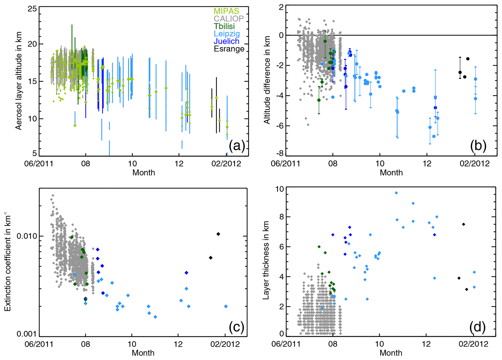
Figure 11Properties of the Nabro sulfate aerosol as a function of time derived from MIPAS (light green), CALIOP (grey), Leipzig lidar (light blue), Jülich lidar (dark blue), Esrange lidar (black), and twilight measurements (dark green). The CALIOP measurements cover the latitude range between 0 and 50∘ N and all ground-based lidar stations are north of 50∘ N. Only for the twilight measurements is there a spatial and temporal overlap with CALIOP. (a) Nabro aerosol layer height measured by all instruments. For MIPAS only the top height is shown. In case of multiple matches for MIPAS the minimum, maximum, and mean top heights derived are shown. (b) Difference between the cloud top heights measured by MIPAS and CALIOP, the ground-based lidars, and the twilight measurements (MIPAS-lidar/twilight) during the 8 months after the Nabro eruption. If more than one MIPAS profile was within the match range, the circles indicate the average and the bars the range of the individual profiles. (c) Nabro aerosol layer extinction coefficient at 532 nm derived from the lidar and twilight measurements between June 2011 and February 2012. For the Jülich lidar and the twilight measurements the data were scaled to 532 nm. (d) Nabro aerosol layer thickness derived from the lidar and twilight measurements from June 2011 to February 2012.
In the comparison of the top heights (Fig. 11a) we see a decrease with time and when moving from low (CALIOP and twilight) to high latitudes (ground-based lidars). Compared to the Leipzig lidar measurements we found that MIPAS underestimates the aerosol layer top height in all matches (Fig. 11b). The underestimation ranges from 0.9 to 7.2 km and is 3.4 km in mean and 3.1 km in median. From the simulations we derived that these underestimations can be expected for extinction coefficients smaller than km−1 at 10.5 µm, which is smaller than about km−1 at 532 nm. The average layer extinction coefficients for the nighttime measurements range from to km−1 assuming a lidar ratio of 50, as for the CALIOP measurements (Fig. 11c). These extinction coefficients are below or close to the lowest aerosol detection limit that we derived from the simulations for MIPAS. Our simulations indicate that aerosol layers with low extinctions are only detectable if they are thicker than 1 km and that a significant top height underestimation can be expected. The accumulated vertical extent of the aerosol layers above 7 km, which is approximately the lowest MIPAS tangent altitude within the match radius around Leipzig, ranges from 1.9 to 9.6 km (Fig. 11d). The comparison of the aerosol layer top heights between MIPAS and the Leipzig lidar is consistent with the findings from the simulations. Between July and November 2011 we observe a decrease in extinction coefficient, an increase in layer thickness, and consequently an increase in top height difference.
The gradient method following Mattis et al. (2008) was used to derive the layer top height, because the Leipzig lidar has a higher sensitivity towards aerosol than CALIOP and consequently the extinction threshold method would miss layers with low extinctions. The sensitivity to the method used to derive the top height we investigated with the three selected nighttime profiles in Fig. 10, since extinction coefficients were only available for the nighttime measurements. Using the extinction coefficient threshold of km−1, the top heights became 0.7 km lower in the first case, 3.1 km lower in the second case, and 6.0 km lower in the third case (Table 6). Consequently, this leads to smaller top height differences compared to MIPAS, −0.4 to −0.7 km in the first case and −1.2 to −3.8 km in the second case. The third case would have been excluded from the comparison, because the top layer is below the extinction threshold and the bottom layer top height is below the lowest MIPAS tangent altitude of about 7 km around Leipzig. Using the extinction threshold method would bring the altitude difference, mean extinction, and layer thickness closer to the bulk of the CALIOP measurements in Fig. 11.
Table 6Cloud top heights of the Nabro sulfate aerosol measured by the Leipzig lidar using the gradient method and the extinction threshold method.
The finding that the gradient method derives higher top heights for ground-based lidar than the extinction threshold method is in contrast to the finding for CALIOP, where the gradient method derived lower top heights. One contribution to this discrepancy is that for CALIOP we only considered the maximum gradient of the entire profile, which is only correct under the assumption of a single layer, and hence in some cases missed a thinner layer with a smaller gradient above, whereas for each Leipzig lidar profile a more sophisticated and visual analysis was performed that provided multiple layer structures. Another contribution to this discrepancy is the difference in the sensitivity of the ground-based and space-based lidar profiles. While for the CALIOP profiles the average layer extinction was always larger than km−1 to be clearly detectable, the average layer extinction of the Leipzig lidar profiles was mostly below km−1.
In several cases there was more than one MIPAS profile within the match range (Fig. 10). Although the MIPAS cloud top height often is not the first tangent altitude within the aerosol layer (Fig. 10), we observe that the profiles are noisy above the aerosol layer but get aligned with the first tangent altitude within the aerosol layer. Even if there is no MIPAS aerosol detection, we observe a clear aerosol signal in the MIPAS ACI profiles that are aligned within the aerosol layer (Fig. 10c).
Table 7Nabro sulfate aerosol measured by the Jülich lidar and MIPAS. For the lidar data aerosol layer top, bottom, and mean extinctions at 355 nm are given. For MIPAS, the number of matching profiles, the mean cloud top height, and the corresponding minimum and maximum top heights are given.
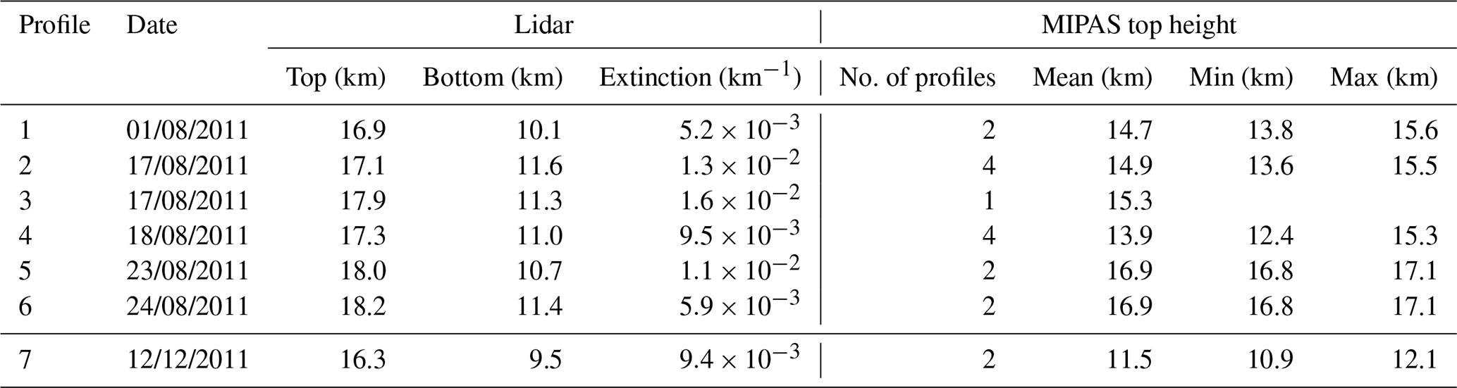
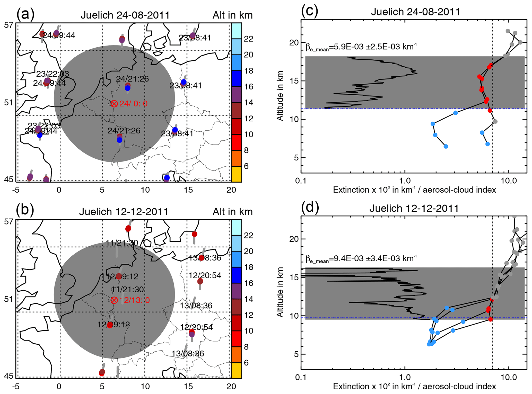
Figure 12Nabro aerosol measured by the Jülich lidar and MIPAS on (a, c) 24 August 2011 and (b, d) 12 December 2011. (a, b) The maps show the lidar station, lidar measurement time, match radius, MIPAS orbits, MIPAS profile measurement time, and MIPAS cloud top heights (colour coded). (c, d) Jülich lidar extinction profile at 355 nm (black line) between aerosol top and bottom altitude (grey box) and MIPAS ACI profiles. In the MIPAS ACI profiles the grey dots denote clear air, red dots sulfate aerosol, and blue dots denote ice and optically thick clouds. The black dotted line is the ACI threshold of 7.
4.5 Jülich lidar measurements
The Jülich cloud lidar in Germany was operated on several days in July, August, and December 2011. The match criteria were the same as for the Leipzig lidar: a match radius of 500 km and a match time of start of the measurement −24 h to end of the measurement +24 h. To achieve a good signal-to-noise ratio the lidar profiles were averaged over measurement periods of 3 to 4 h. In total 10 lidar profiles were available and we found matches with MIPAS aerosol measurements for 7 lidar profiles that were measured on 6 different days (e.g. two examples in Fig. 12). The lidar cloud top and bottom altitudes, average extinction, and the MIPAS minimum, maximum, and mean cloud top heights are given in Table 7 for each match. As already shown for the aged aerosol measured over Leipzig (Fig. 10c), we observe that the MIPAS ACI profiles are directed below the aerosol top, but the ACI threshold (7) is only crossed at altitudes close to the aerosol layer bottom altitude (Fig. 12b).
The comparison of the cloud top heights shows that the MIPAS top heights are always below the lidar top heights, by −0.9 to −5.4 km, but always within the aerosol layer (Fig. 11a). Between August and December 2011 there is an increase in the top height difference, which is in agreement with the results for the Leipzig station (Fig. 11b). The average extinction coefficients at 355 nm are given in Table 7. To make the extinctions comparable to the CALIOP and Leipzig lidar measurements, we derived a scaling factor of 0.46 from the data in Fig. 4 for the particle size distribution measured after the Nabro eruption to scale the 355 nm extinction coefficient to 532 nm. Figure 11c shows that the scaled extinction coefficients between and km−1 are within the range of the CALIOP and Leipzig measurements. The aerosol layer thickness measured in Jülich in August is significantly larger than in the CALIOP measurements (Fig. 11d). This can be attributed to the fact that the CALIOP aerosol data are only available south of 50 ∘ and down to 12 km. The profiles often terminate already around 15 km due to ice clouds, whereas the Jülich profiles cover the extra-tropical stratosphere and the troposphere down to the ground.
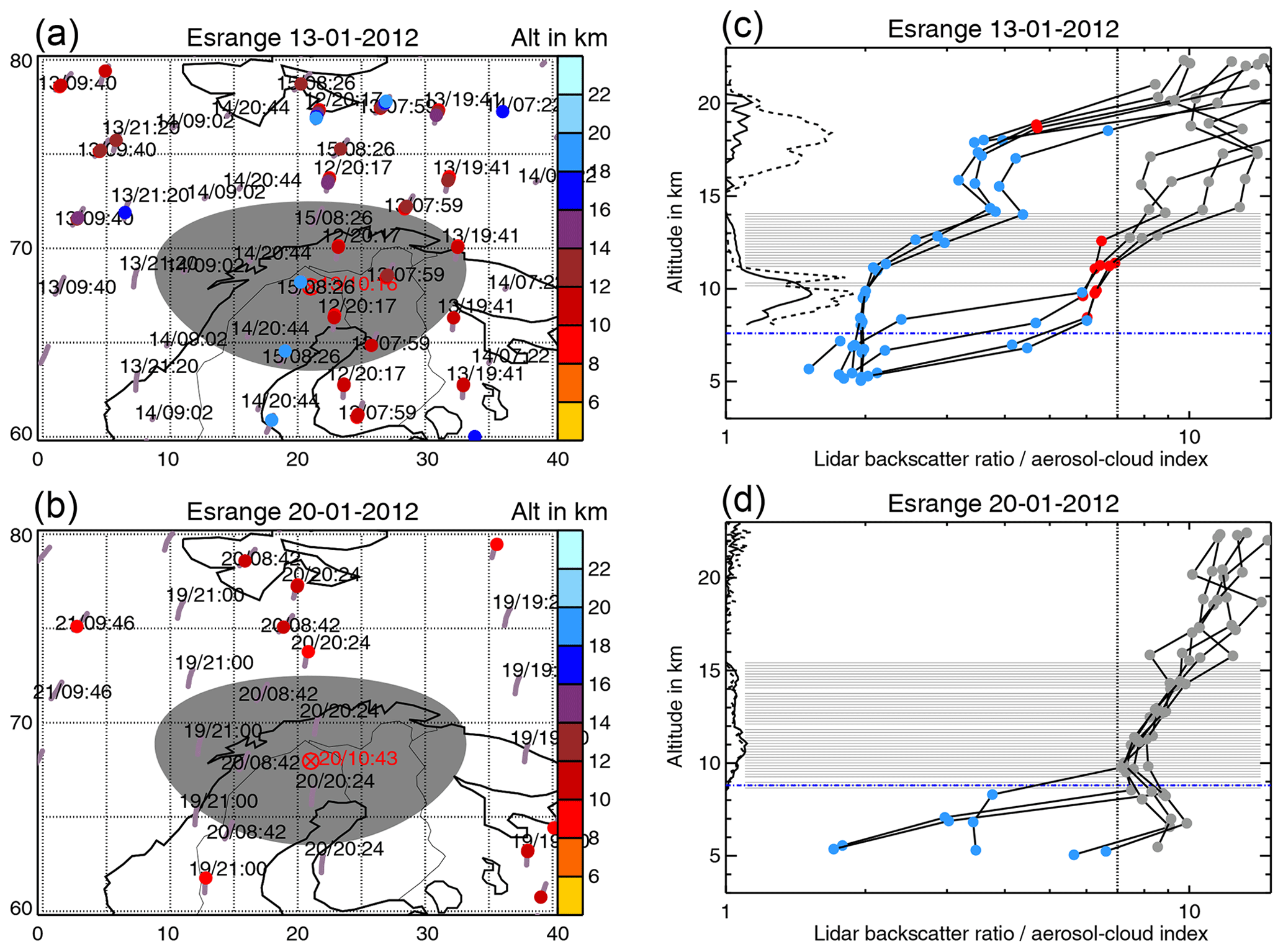
Figure 13Nabro aerosol measurements over Esrange on (a, c) 13 January 2012 and (b, d) 20 January 2012. (a, b) Maps with lidar station, lidar measurement time, match radius, MIPAS orbits, MIPAS profile measurement time, and MIPAS cloud top heights (colour coded). (c, d) MIPAS ACI profiles and lidar backscatter ratio profiles. The grey areas denote the aerosol layer measured by the lidar, the black solid line is the parallel backscatter ratio, and the black dashed line is the perpendicular backscatter ratio. In the MIPAS ACI profiles the grey dots denote clear air, red dots sulfate aerosol, and blue dots denote ice and optically thick clouds. The black dotted line is the ACI threshold of 7.
A sensitivity test using an extinction coefficient threshold to identify the aerosol layer top height did not work, because the extinction profiles were very noisy in the stratosphere and often reach the threshold at the uppermost tangent altitude.
4.6 Esrange lidar measurements
The Esrange lidar in northern Sweden was operated on 8 d between 6 and 25 January 2012 in order to measure PSCs. We applied the same match criteria as for the Leipzig and Jülich lidars: a match radius of 500 km and a match time of the start of the measurement −24 h to the end of the measurement +24 h. PSCs have a strong impact on MIPAS measurements and the signal of the aerosol layer is disturbed by the PSC signal (as seen in Fig. 13a). Hence, we excluded all matching MIPAS profiles that were affected by PSCs. Finally we found three lidar profiles (13, 19, 23) with matching unperturbed MIPAS profiles (e.g. Fig. 13).
Table 8Nabro sulfate aerosol measured by the Esrange lidar and MIPAS. For the lidar data aerosol layer top and bottom are given. For MIPAS, the number of matching profiles, the mean cloud top height, and the corresponding minimum and maximum top heights are given.

For the Esrange lidar only the parallel and perpendicular backscatter ratios were available. To determine the sulfate aerosol layer we considered all measurements where the parallel backscatter signal was larger than 1.003. In a second step we filtered out PSCs above 17 km and ice clouds where the perpendicular backscatter signal is larger than the parallel backscatter signal due to solid particles (e.g. Fig. 13a). We also applied the gradient method (Sect. 4.4) to the parallel backscatter profiles. In those cases where a clear variation in the gradient was present the cloud top heights of both methods agree. However, due to the low particle concentrations in aerosol layers, the gradient method did not provide results in all cases (Mattis et al., 2008). For the three matches the lidar top and bottom altitudes, average extinction, and the MIPAS minimum, maximum, and mean top heights are given in Table 8.
In the first match on 13 January 2012 (Fig. 13a) the lidar profile also shows solid PSC particles in the stratosphere and three out of seven MIPAS profiles within the match radius also detected these PSCs. However, four profiles were not affected by the PSCs. For all matches, the aerosol layer top height detected by MIPAS is 1.5–2.8 km below the top height derived from the lidar measurement (lidar measurement altitude error ±150 m). The aerosol layer thickness reaches from about 3 to 7.5 km, which is within the wide range found by the Leipzig lidar (Fig. 11d). Figure 13b shows a match between PSC-free lidar and MIPAS profiles on 20 January 2012. Although the MIPAS ACI profiles do not cross the detection threshold the aerosol layer signal is clearly visible (noisy profiles above the aerosol layer and aligned profiles with a local ACI minimum within the layer). For 2 d it was possible to derive an average extinction coefficient from the 532 nm lidar data that is shown in Fig. 11c as a representative for the Esrange data.
Table 9Nabro sulfate aerosol measured by the twilight technique, MIPAS, and CALIOP over Tbilisi. For the twilight data the aerosol layer top and bottom altitudes, the corresponding errors, and the averaged extinction coefficient are given. For CALIOP the aerosol layer top, bottom, and average extinctions are given. For MIPAS, the number of matching profiles, the mean cloud top height, and the corresponding minimum and maximum top heights are given.
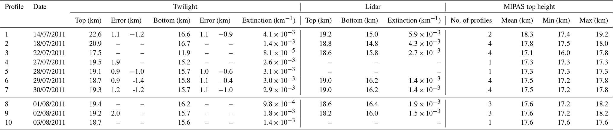
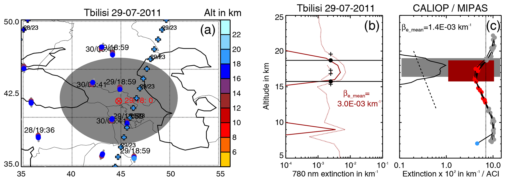
Figure 14Measurements of Nabro aerosol over Tbilisi on 29 July 2011. (a) Map with the twilight station, match radius, MIPAS and CALIPSO orbits, their measurement times, and the MIPAS (circles) and CALIOP (crosses) cloud top heights (colour coded). (b) Twilight extinction profile at 780 nm (red solid line) and uncertainty (red dotted lines). The black circles indicate the aerosol layer top and bottom altitude and the black crosses indicate the altitude uncertainty range. (c) CALIOP extinction (black solid line) and MIPAS ACI profiles (black lines with coloured circles). For the CALIOP profile the black dashed line indicates the extinction threshold and the grey box is the aerosol layer derived from CALIOP. For the MIPAS profiles grey dots denote clear air, red dots sulfate aerosol, and blue dots denote ice and optically thick clouds. The black dotted line is the ACI threshold of 7. The red box denotes the aerosol layer detected by the twilight measurement.
4.7 Tbilisi twilight measurements
The match criteria for the comparison of the twilight profiles with MIPAS profiles were the same as for the lidar measurements: 500 km match radius and a match time of 18:00 UTC ±24 h (an approximate time of evening twilights in summer). All MIPAS profiles within the match range were compared individually to the twilight profiles. In addition, we applied the same match criteria to CALIOP measurements and added the averaged lidar profile to the comparison (Fig. 14a, c). For the 11 twilight profiles measured between 14 July and 3 August 2011 we found matches with MIPAS aerosol measurements for 10 profiles and for CALIOP aerosol measurements we found matches for 8 profiles (Table 9).
For each twilight profile the top and bottom altitudes of the Nabro aerosol layer were estimated at extinction maximum half width. The top and bottom altitude uncertainty ranges are given by the intersection of the extinction at maximum half width with the ± extinction error profiles (Fig. 14b). While for all twilight profiles aerosol layer top and bottom heights could be derived, the full set of uncertainty ranges could be derived only for four profiles. The twilight top and bottom heights, the corresponding uncertainty ranges, the average layer extinction coefficient, the CALIOP top and bottom heights, the average CALIOP layer extinction coefficient, and the MIPAS cloud top heights are given in Table 9.
The differences between the twilight and MIPAS cloud top heights range from −5.2 to +0.3 km (Fig. 11b and Table 9). In all cases but one the MIPAS cloud top height is below the twilight cloud top height. Although for this particular measurement no error estimate is available for the twilight measurement, assuming an error of 2 km from the other profiles the MIPAS and twilight top heights agree within the error range. Compared to CALIOP, the MIPAS top heights are always lower or equal. Comparing the twilight to the CALIOP top heights, the twilight top heights are in the range of +3.4 and −1.1 km around the CALIOP top heights. In two cases this is above the twilight uncertainty. Although the twilight measurements have a significantly coarser vertical resolution than the lidar measurements, the cloud top height differences to MIPAS are in the same range as for the lidar measurements (Fig. 11b). Also, the layer thickness derived from the twilight measurements is comparable to the layer thickness derived from the lidars (Fig. 11d). To compare the average layer extinction coefficient we scaled the twilight 780 nm extinction to the 532 nm lidar extinction using a scaling factor of 2.38 derived from Fig. 4 for the particle size distribution measured after the Nabro eruption. Except for 22 July 2011, where the signal was very weak and the extinction coefficient was very low (out of the plot range), the average twilight extinction agrees well with the lidar extinctions (Fig. 11c).
5.1 Detection sensitivity
While Griessbach et al. (2016) showed that MIPAS measurements are sensitive to 1 km thick sulfate aerosol layers with extinction coefficients down to km−1, the simulations in Sect. 3 showed that for 6 km thick layers the detection sensitivity reaches down to km−1. In the comparison with lidar and twilight measurements of the Nabro sulfate aerosol, MIPAS measurements were sensitive towards extinction coefficients of about km−1 at 532 nm (Sect. 4, Fig. 11c), which corresponds to about km−1 at 10.5 µm (see Fig. 4). These extinctions are slightly higher than the lower aerosol and cloud detection limit of about km−1 ( km−1 at 12 µm scaled to 10.5 µm) found by Sembhi et al. (2012) for MIPAS.
Since the extinction coefficients for sulfate aerosol significantly differ between wavelengths in the VIS and IR range and the detection sensitivities of the instruments introduced in Sect. 1 are given at their native wavelengths (Table 1), we used the scaling factors for background aerosol and volcanically enhanced sulfate aerosol with particle sizes larger than 0.1 µm from Fig. 4 and Table 3 to compare the sensitivity range of MIPAS measurements towards sulfate aerosol with established instruments for aerosol detection. The sensitivity ranges given in Table 1, reaching from the lowest detectable extinction to the largest detectable extinction coefficient before becoming optically thick, were scaled to 10.5 µm (950 cm−1) and are shown in Fig. 15. In brief, the solar occultation and scattering techniques provide the highest sensitivity towards sulfate aerosol, but become optically thick at extinctions that are already reached by moderate volcanic eruptions (Fromm et al., 2014). The sensitivities of infrared limb emission measurements and active lidar are comparable and fill the gap in detection sensitivity between solar occultation/scattering and infrared nadir measurements.
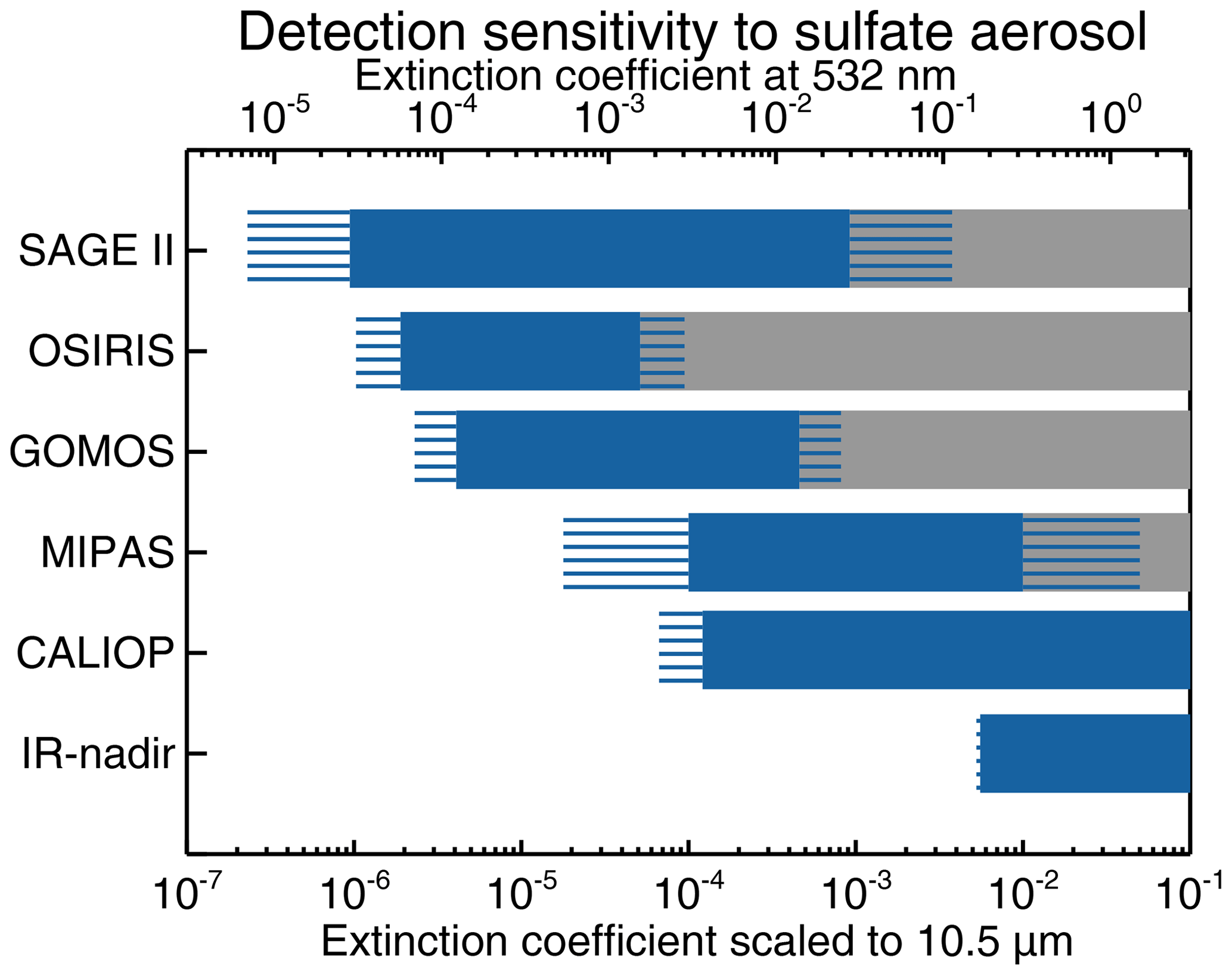
Figure 15Detection sensitivity to sulfate aerosol extinctions for different satellite-based instruments. The blue bars indicate a conservative estimate of detectable extinctions given in Table 1 and scaled to 950 cm−1. The grey bars indicate detectable but optically thick extinctions. The blue stripes indicate the uncertainties due to the scaling factor for SAGE II and IR nadir. For MIPAS, CALIOP, GOMOS, and OSIRIS the blue stripes are a combination of uncertainties due to the scaling factor and less conservative detection thresholds (lower minimum extinctions) given in the literature. For CALIOP only the nighttime extinctions are considered. Further details on the instruments' measurement capabilities and the corresponding references are given in Table 1.
5.2 Top height
The simulation results showed that for MIPAS the measured cloud top heights strongly depend on the layer extinction coefficient. For extinction coefficients of km−1 (at 10.5 µm) and smaller there is a strong tendency towards underestimation of the cloud top height, whereas for larger extinctions there is a strong tendency towards overestimation (Fig. 2). The extinction coefficients of the Nabro aerosol used for the comparison in this study range from to km−1 at 532 nm (Fig. 11c), which corresponds to about and km−1 at 10.5 µm. For this range of extinction coefficients the simulations (Sect. 3) predict a possible overestimation of up to about 1 km and possible underestimations of up to 5.1 km (Fig. 2). The cloud top height differences deduced from the comparison of MIPAS to the lidar and twilight measurements between June and October 2011 (Fig. 11b) are in agreement with the results from the simulations, with an average underestimation of about 1 km by MIPAS, an overestimation in about 5 % of the cases of mostly below 1 km, and an underestimation of less than 5 km in most cases. From October 2011 on the altitude differences start to exceed −5 km. In most of these cases the extinction coefficient is smaller than the lowest simulated extinction coefficient in Fig. 2, but the measured layer thickness is larger than 6 km, which was the thickest layer assumed in the simulations. Hence, the comparisons of MIPAS measurements with lidar measurements indicate that the simulation results may be extrapolated towards thicker aerosol layers and smaller extinctions and consequently will lead to even larger top height underestimations. However, although the aerosol layers detected in the observations and discussed here can be considered sufficiently extended and homogeneous, we cannot rule out that some of the larger underestimations can also be attributed to broken cloud conditions. Considering the negative offset of about 0.3 to 0.5 km on average of the MIPAS engineering tangent heights (Kleinert et al., 2018), there would still be an average underestimation of 0.7 to 0.5 km. Further, the majority of the compared profiles would still fall within the ranges predicted by the simulations.
Previous comparisons of MIPAS cloud top heights led to contradictory results. For cirrus clouds and aerosol Sembhi et al. (2012) found an overestimation of the cloud top height of up to 1 km in comparison to HIRDLS and CALIOP and Spang et al. (2012) found an overestimation of occasionally more than 2 km for MIPAS in comparison to the GLAS lidar. Spang et al. (2012) also found an underestimation of up to 2.5 km for sub-visible cirrus (SVC) cloud top heights in comparison to SAGE II top heights. Further, Höpfner et al. (2009) reported an underestimation of up to 2.5 km in comparison to CALIOP for PSC top heights. These seemingly contradictory results can be reconciled when considering the characteristic extinction coefficients of the compared cloud data sets.
To make our results for the ACI detection method comparable to previous studies that used the CI for cloud detection, we also performed the entire analysis for the CI using slightly modified altitude- and latitude-variable thresholds (Griessbach et al., 2018) following Sembhi et al. (2012). The CI shows a slightly higher sensitivity towards ice and a slightly lower sensitivity towards aerosol, but most importantly here, it systematically estimates the cloud top height 0.1 km higher than the ACI.
PSCs are optically relatively thin, with 532 nm extinctions between about 1 and 2 km−1 (Pitts et al., 2018), so that only CALIPSO nighttime measurements are used to analyse PSCs (Pitts et al., 2009). Höpfner et al. (2009) discussed several effects, e.g. horizontal shifts of the PSC relative to the tangent point, the horizontal cloud extent, and diffuse boundaries as possible causes of the underestimation. Yet none of these reasons could explain the variations with altitude (Höpfner et al., 2009). They speculated that rather patchier PSC structures at higher altitudes are causing the higher underestimations than an altitude-dependent sensitivity towards PSCs. However, based on our results a low PSC extinction coefficient alone can be sufficient to explain underestimations of the cloud top height of up to 2.5 km in the UTLS and even more at altitudes above about 21 km, where the MIPAS vertical sampling is increased to 3 km.
For the comparison of tropospheric clouds between 50∘ N and 50∘ S and 12 to 20 km altitude, Sembhi et al. (2012) calculated 3-monthly averages for 5∘ latitude and 10∘ longitude grid boxes using the altitude- and latitude-dependent CI thresholds that are also sensitive to PSCs and aerosol. However, to exclude volcanic aerosol, Sembhi et al. (2012) selected two 3-monthly intervals relatively free of volcanic aerosol, JJA 2007 and DJF 2007/2008. This means that this data set mainly contains optically thick clouds in the mid-IR and a smaller fraction of optically thin clouds around the tropopause. From our simulations cloud top height differences between −0.2 and 1.6 km can be expected for optically thick clouds with extinction coefficients larger than km−1. This is in agreement with the differences to CALIOP and HIRDLS found by Sembhi et al. (2012). The differences in the 3-monthly averaged grid boxes reached up to 1 km compared to CALIOP and on average the cloud top heights were 0.75 km higher for MIPAS than for CALIOP and HIRDLS.
In another comparison of tropospheric clouds between 50∘ N and 50∘ S Spang et al. (2012) investigated matches between MIPAS and GLAS lidar profiles between September and November 2003, when the MIPAS vertical sampling was 3 km. The results, given as mean differences in 3 km altitude bins, show that MIPAS systematically overestimated the cloud top height by mostly less than 2 km (Spang et al., 2012, Fig. 18). Based on our results, we expected an overestimation for tropospheric clouds of up to 1.6 km. In the same study PSCs were also included at latitudes poleward of 50∘. For PSCs overestimations of the cloud top height of more than 5 km were found compared to GLAS. Such a high overestimation is in clear contradiction to the tendency towards underestimation found by Höpfner et al. (2009) for PSCs with respect to CALIOP and also cannot be explained by field-of-view effects. Spang et al. (2012) suggested a smaller sensitivity of GLAS measurements towards optically thin PSCs and inhomogeneities in the PSC fields as causes of the larger differences. Using less sensitive cloud detection methods for MIPAS, the overestimation compared to GLAS was reduced (Spang et al., 2012). Hence, we consider GLAS measurements not sufficiently sensitive toward optically thin clouds to be useful for a comparison with MIPAS cloud measurements.
For the particular case of sub-visible cirrus Spang et al. (2012) compared different cloud detection algorithms for MIPAS to SAGE II sub-visible cirrus detections. The comparison of zonal 3-monthly means measured in 2003 showed that outside the polar vortex most methods systematically underestimated the cloud top height by up to 2.5 km compared to SAGE II (Spang et al., 2012, Fig. 12). Inside the polar vortex the MIPAS data include PSCs, whereas the SAGE II sub-visible cirrus data set does not. Only the MIPAS cloud top height based on altitude- and latitude-variable thresholds by Sembhi et al. (2012) overestimated the SAGE II cloud top heights in many cases. This overestimation, however, was attributed to an underestimation of the cloud occurrence at lower altitudes that led to a higher average cloud top height for this method (Spang et al., 2012). Both the overestimations and the underestimations were considered to be within the range of the vertical sampling that was 3 km in 2003. Yet, considering the extinction coefficients that are between and km−1 for SAGE II sub-visible cirrus, we argue that a systematic underestimation of cloud top height by MIPAS can also be caused by the rather small extinction coefficients of sub-visible cirrus. In contrast to sulfate aerosol the SAGE II 1020 nm extinction coefficients for ice can be scaled to the mid-IR using a scaling factor of approximately 1. As Fig. 2 shows, top height underestimations of up to 2.4 km are possible for a vertical sampling of 1.5 km, which increases to about 3.9 km at 3 km vertical sampling, while only overestimations of up to 1.6 km are possible. Spang et al. (2012) compared the cloud top heights of individual profiles and presented the results in 3 km altitude bins. They found an overestimation of up to 1 km in the topmost altitude bin and underestimations of up to 1, 3, and 5 km in the following altitude bins below. Based on our simulations all these values are well within the range that can be expected for the extinction coefficients of sub-visible cirrus.
In this study we characterised the cloud top height information from Envisat MIPAS measurements. In the first step radiative transfer simulations that account for scattering on ice, volcanic ash, and sulfate aerosol particles were performed and evaluated. In the simulated scenarios MIPAS measurements were shown to be sensitive to sulfate aerosol down to an extinction coefficient of km−1 at 10.5 µm. The sensitivity was positively correlated with the vertical thickness of the cloud layer. A larger vertical extent of the cloud leads to a smaller lower detection threshold due to a larger fraction covered with cloud within MIPAS' vertical field-of-view. The dependency of the detection sensitivity on the extinction coefficient and cloud-covered field-of-view fraction affected the derived cloud top height. For optically thick clouds ( km−1), such as cirrus clouds that lead to a constant ACI profile at all altitudes below the cloud, the cloud top height can be overestimated by up to 1.6 km due to MIPAS' broad field-of-view. In contrast, for optically thin clouds ( km−1), such as sulfate aerosol, PSCs, and sub-visible cirrus that cause a pronounced minimum in the ACI profile with minimum values of about 5.5 or larger, the cloud top height can be underestimated by up to 5.1 km, which is a combination of the field-of-view effect and the low extinction. For minimum ACI values between 3 and 5.5 both overestimation and underestimation of the cloud top height are possible. Further, MIPAS' coarse vertical sampling of 1.5 km contributes to the large derived top height uncertainty ranges.
In the second step MIPAS measurements of volcanic sulfate aerosol from the Nabro eruption were compared with lidar and twilight measurements. MIPAS detected the Nabro aerosol between the eruption in June 2011 until the end of its lifetime in April 2012. Nabro aerosol measurements were available from June to August from CALIOP single profiles, in July and August 2011 from twilight measurements, and between July 2011 and February 2012 from ground-based lidar measurements. The lidar and twilight data show that while the average Nabro aerosol extinction coefficient (at 532 nm) in June and July was larger than km−1 and the layer thickness was mostly below 4 km, the average extinction coefficient decreased with time and the layer thickness increased to 9.5 km (Fig. 11).
Making the inherently different measurements of the aerosol layer top height comparable required an assessment of the sensitivities of the various top height estimation methods. Therefore Mie scattering simulations for measured volcanic sulfate aerosol particle size distributions were used to scale the MIPAS IR detection threshold ( km−1) to the lidar and twilight wavelengths. For sulfate aerosol the extinction coefficient in the visible is more than 1 order of magnitude (a factor of about 30) larger than in the mid-IR at 10.5 µm. Hence, an altitude-variable extinction threshold (Winker et al., 2009) that has an extinction coefficient of km−1 at 18 km was used as a threshold for the cloud top height derived from CALIOP. This threshold was confirmed by a sensitivity test analysing the number of matches between CALIOP and MIPAS aerosol detections for varying thresholds. For up to 2 months of Nabro aerosol measured by CALIOP, the commonly used gradient method (Mattis et al., 2008) for aerosol layer top estimation from lidar measurements resulted in 55.1 % at the same (2 km) top height as the extinction coefficient threshold of km−1, while in 7.7 % the top height was higher and in 37.2 % it was lower. In contrast, for the aged volcanic aerosol plume measured by the ground-based lidars the average plume extinction was below km−1, and here the gradient method led to significantly higher top heights or even allowed for the detection of thinner layers that would have been missed using the extinction threshold.
As the extinction coefficient of the Nabro plume was low in general, MIPAS underestimated the aerosol layer top height. Compared to the CALIOP measurements that due to its lower sensitivity limit detected the plume mostly in the first 2 months after the eruption, the MIPAS measurements underestimated the aerosol layer top height in 84 %–95 % of all matches by 0.9 km on average. For the ground-based lidar measurements of the aged and dispersed plume with extinction coefficients below km−1 (at 532 nm, which corresponds to km−1 at 10.5 µm), the MIPAS measurements always underestimated the aerosol layer top height by at least 0.9 and up to 7.2 km. Compared to the twilight measurements that have an overlap with the CALIOP measurements, the MIPAS measurements underestimated the cloud top height by up to 5.2 km in all but one case, where an overestimation of 0.3 km was found. The results of this comparison are consistent with each other and in good agreement with the simulations predicting the underestimation of the cloud top height for low extinctions. Moreover, the comparison indicates that MIPAS can be sensitive to even lower extinctions ( km−1 at 10.5 µm) if the vertical thickness of the cloud layer is larger than the 6 km considered in the simulations, here.
Our results show that in addition to the known causes of cloud top height uncertainties in IR limb emission measurements, namely the overestimation due to a large field-of-view and the underestimation due to broken cloud conditions, the extinction coefficient of the aerosol or cloud layer also has an impact on the derived cloud top height. Previous studies showing MIPAS overestimating and/or underestimating cloud top heights were found to be not contradictory, but rather complementary to each other as they investigated different cloud types covering a large range of characteristic extinction coefficients. The overestimations and underestimations of cloud top height in previous studies can be explained by the effect of the cloud extinction coefficient and the vertical field-of-view. Since for MIPAS measurements reliable algorithms are available to discriminate between ice clouds and aerosol and to filter out optically thick profiles, the altitude uncertainty ranges can be narrowed down for each group. Although MIPAS' vertical sampling is relatively coarse and the altitude uncertainty is large compared to e.g. CALIPSO and SAGE II, MIPAS' vertically resolved aerosol and cloud measurements provide additional information by covering the entire Earth from pole to pole at daytime and nighttime and even fill gaps in the sensitivity towards aerosol and cloud particles covering a wide range of extinctions.
JURASSIC is freely available at https://jugit.fz-juelich.de/slcs/jurassic-scatter (Jülich Supercomputing Centre, Forschungszentrum Jülich GmbH, 2020). Refractive indices used for the simulations are available from the HITRAN compilation at http://hitran.org (Atomic and Molecular Physics Division, Harvard-Smithsonian Center for Astrophysics, 2020). The MIPAS level 1b IPF version 7.11 data can be accessed after registration via ESA's Earth Online portal https://earth.esa.int/web/guest (ESA, 2020). The MIPAS CI, ACI, aerosol, ash, and cloud detections are available at https://datapub.fz-juelich.de/slcs (Forschungszentrum Jülich GmbH, 2020).
SG designed and performed the study. LH and RS contributed to the setup and analysis of the radiative transfer simulations for MIPAS. PS prepared and provided the Leipzig lidar data. CR prepared and provided the Jülich lidar data. PA prepared and provided the Esrange lidar data. NM prepared and provided the Tbilisi twilight data. JPV prepared and provided the CALIOP lidar data. SG wrote the paper with contributions from all the coauthors.
The authors declare that they have no conflict of interest.
The authors gratefully acknowledge the computing time granted through JARA-HPC on the JURECA supercomputer at Forschungszentrum Jülich. The authors thank Anu Dudhia for providing the Reference Forward Model (RFM) that was used to generate the look-up tables for JURASSIC. The MIPAS level 1b IPF version 7.11 data were provided by the European Space Agency (ESA) and the analysis of the simulation results was supported by ESA within the framework of the “Particulate matter in the upper troposphere and stratosphere” project. Finally, we thank two anonymous reviewers for their helpful comments.
This research has been supported by the European Space Agency (grant no. 400011677/16/NL/LvH).
The article processing charges for this open-access
publication were covered by a Research
Centre of the Helmholtz Association.
This paper was edited by Andrew Sayer and reviewed by two anonymous referees.
Achtert, P., Khaplanov, M., Khosrawi, F., and Gumbel, J.: Pure rotational-Raman channels of the Esrange lidar for temperature and particle extinction measurements in the troposphere and lower stratosphere, Atmos. Meas. Tech., 6, 91–98, https://doi.org/10.5194/amt-6-91-2013, 2013. a, b
Ackerman, S. A.: Remote sensing aerosols using satellite infrared observations, J. Geophys. Res., 102, 17069–17079, https://doi.org/10.1029/96JD03066, 1997. a, b
Ansmann, A., Wandinger, U., Riebesell, M., Weitkamp, C., and Michaelis, W.: Independent measurement of extinction and backscatter profiles in cirrus clouds by using a combined Raman elastic-backscatter lidar, Appl. Optics, 31, 7113–7131, 1992. a, b
Antuña, J. C., Robock, A., Stenchikov, G. L., Thomason, L. W., and Barnes, J. E.: Lidar validation of SAGE II aerosol measurements after the 1991 Mount Pinatubo eruption, J. Geophys. Res., 107, ACL 3-1–ACL 3-11, https://doi.org/10.1029/2001JD001441, 2002. a, b, c, d
Atomic and Molecular Physics Division, Harvard-Smithsonian Center for Astrophysics: HITRANonline, available at: http://hitran.org, last access: 19 February 2020. a
Bauman, J. J., Russell, P. B., Geller, M. A., and Hamill, P.: A stratospheric aerosol climatology from SAGE II and CLAES measurements: 2. Results and comparisons, 1984–1999, J. Geophys. Res., 108, 4383, https://doi.org/10.1029/2002JD002993, 2003. a
Bertaux, J. L., Kyrölä, E., Fussen, D., Hauchecorne, A., Dalaudier, F., Sofieva, V., Tamminen, J., Vanhellemont, F., Fanton d'Andon, O., Barrot, G., Mangin, A., Blanot, L., Lebrun, J. C., Pérot, K., Fehr, T., Saavedra, L., Leppelmeier, G. W., and Fraisse, R.: Global ozone monitoring by occultation of stars: an overview of GOMOS measurements on ENVISAT, Atmos. Chem. Phys., 10, 12091–12148, https://doi.org/10.5194/acp-10-12091-2010, 2010. a
Blum, U. and Fricke, K. H.: The Bonn University lidar at the Esrange: technical description and capabilities for atmospheric research, Ann. Geophys., 23, 1645–1658, https://doi.org/10.5194/angeo-23-1645-2005, 2005. a
Bourassa, A. E., Rieger, L. A., Lloyd, N. D., and Degenstein, D. A.: Odin-OSIRIS stratospheric aerosol data product and SAGE III intercomparison, Atmos. Chem. Phys., 12, 605–614, https://doi.org/10.5194/acp-12-605-2012, 2012a. a, b
Bourassa, A. E., Robock, A., Randel, W. J., Deshler, T., Rieger, L. A., Lloyd, N. D., Llewellyn, E. J. T., and Degenstein, D. A.: Large Volcanic Aerosol Load in the Stratosphere Linked to Asian Monsoon Transport, Science, 337, 78–81, https://doi.org/10.1126/science.1219371, 2012b. a, b, c, d
Casadevall, T.: The 1989–1990 eruption of Redoubt volcano, Alaska – impacts on aircraft operations, J. Volcanol. Geoth. Res., 62, 301–316, https://doi.org/10.1016/0377-0273(94)90038-8, 1994. a
Castelli, E., Dinelli, B. M., Carlotti, M., Arnone, E., Papandrea, E., and Ridolfi, M.: Retrieving cloud geometrical extents from MIPAS/ENVISAT measurements with a 2-D tomographic approach, Opt. Express, 19, 20704–20721, https://doi.org/10.1364/OE.19.020704, 2011. a
Clarisse, L., Hurtmans, D., Prata, A. J., Karagulian, F., Clerbaux, C., De Maziere, M., and Coheur, P.-F.: Retrieving radius, concentration, optical depth, and mass of different types of aerosols from high-resolution infrared nadir spectra, Appl. Optics, 49, 3713–3722, 2010. a
Clarisse, L., Coheur, P.-F., Prata, F., Hadji-Lazaro, J., Hurtmans, D., and Clerbaux, C.: A unified approach to infrared aerosol remote sensing and type specification, Atmos. Chem. Phys., 13, 2195–2221, https://doi.org/10.5194/acp-13-2195-2013, 2013. a
Crutzen, P. J.: Albedo enhancements by stratospheric sulfur injections: a contribution to resolve a policy dilemma? An Editorial Essay, Clim. Change, 77, 211–219, 2006. a
Deshler, T., Adriani, A., Gobbi, G. P., Hofmann, D. J., Di Donfrancesco, G., and Johnson, B. J.: Volcanic aerosol and ozone depletion within the Antarctic polar vortex during the Austral spring of 1991, Geophys. Res. Lett., 19, 1819–1822, 1992a. a, b
Deshler, T., Hofmann, D. J., Johnson, B. J., and Rozier, W. R.: Balloon-borne measurements of the Pinatubo aerosol size distribution and volatility at Laramie, Wyoming during the summer of 1991, Geophys. Res. Lett., 19, 199–202, 1992b. a, b
Deshler, T., Johnson, B. J., and Rozier, W. R.: Balloonborne measurements of Pinatubo aerosol during 1991 and 1992 at 41 degrees N – Vertical profiles, size distribution, and volatility, Geophys. Res. Lett., 20, 1435–1438, 1993. a, b
Deshler, T., Larsen, N., Weissner, C., Schreiner, J., Mauersberger, K., Cairo, F., Adriani, A., Di Donfrancesco, G., Ovarlez, J., Ovarlez, H., Blum, U., Fricke, K. H., and Dornbrack, A.: Large nitric acid particles at the top of an Arctic stratospheric cloud, J. Geophys. Res., 108, 4167, https://doi.org/10.1029/2003JD003479, 2003. a
Diallo, M., Ploeger, F., Konopka, P., Birner, T., Müller, R., Riese, M., Garny, H., Legras, B., Ray, E., Berthet, G., and Jegou, F.: Significant Contributions of Volcanic Aerosols to Decadal Changes in the Stratospheric Circulation, Geophys. Res. Lett., 44, 10780–10791, https://doi.org/10.1002/2017GL074662, 2017. a, b
Doeringer, D., Eldering, A., Boone, C. D., González Abad, G., and Bernath, P. F.: Observation of sulfate aerosols and SO2 from the Sarychev volcanic eruption using data from the Atmospheric Chemistry Experiment (ACE), J. Geophys. Res., 117, D03203, https://doi.org/10.1029/2011JD016556, 2012. a
ESA: Earth Online, available at: https://earth.esa.int/web/guest, last access: 19 February 2020. a
Fairlie, T. D., Vernier, J.-P., Natarajan, M., and Bedka, K. M.: Dispersion of the Nabro volcanic plume and its relation to the Asian summer monsoon, Atmos. Chem. Phys., 14, 7045–7057, https://doi.org/10.5194/acp-14-7045-2014, 2014. a
Fischer, H., Birk, M., Blom, C., Carli, B., Carlotti, M., von Clarmann, T., Delbouille, L., Dudhia, A., Ehhalt, D., Endemann, M., Flaud, J. M., Gessner, R., Kleinert, A., Koopman, R., Langen, J., López-Puertas, M., Mosner, P., Nett, H., Oelhaf, H., Perron, G., Remedios, J., Ridolfi, M., Stiller, G., and Zander, R.: MIPAS: an instrument for atmospheric and climate research, Atmos. Chem. Phys., 8, 2151–2188, https://doi.org/10.5194/acp-8-2151-2008, 2008. a, b, c
Forschungszentrum Jülich GmbH: Simulation Laboratory “Climate Science”, Data Repositories, available at: https://datapub.fz-juelich.de/slcs, last access: 19 February 2020. a
Fromm, M., Nedoluha, G., and Charvat, Z.: Comment on “Large Volcanic Aerosol Load in the Stratosphere Linked to Asian Monsoon Transport”, Science, 339, pp. 647, https://doi.org/10.1126/science.1228605, 2013. a
Fromm, M., Kablick III, G., Nedoluha, G., Carboni, E., Grainger, R., Campbell, J., and Lewis, J.: Correcting the record of volcanic stratospheric aerosol impact: Nabro and Sarychev Peak, J. Geophys. Res., 119, 10343–10364, https://doi.org/10.1002/2014JD021507, 2014. a, b, c, d
Goitom, B., Oppenheimer, C., Hammond, J., Grandin, R., Barnie, T., Donovan, A., Ogubazghi, O., Yohannes, E., Kibrom, G., Kendall, M., Carn, S., Fee, D., Sealing, C., Blundy, J., Hamlyn, J., Keir, D., Ayele, A., Wright, T., and Berhe, S.: First recorded eruption of Nabro volcano, Eritrea, 2011, B. Volcanol., 77, 85, https://doi.org/10.1007/s00445-015-0966-3, 2015. a
Gordley, L. L. and Russell, J. M.: Rapid inversion of limb radiance data using an emissivity growth approximation, Appl. Optics, 20, 807–813, 1981. a
Griessbach, S., Hoffmann, L., Hoepfner, M., Riese, M., and Spang, R.: Scattering in infrared radiative transfer: A comparison between the spectrally averaging model JURASSIC and the line-by-line model KOPRA, J. Quant. Spectrosc. Ra., 27, 102–118, https://doi.org/10.1016/j.jqsrt.2013.05.004, 2013. a
Griessbach, S., Hoffmann, L., Spang, R., and Riese, M.: Volcanic ash detection with infrared limb sounding: MIPAS observations and radiative transfer simulations, Atmos. Meas. Tech., 7, 1487–1507, https://doi.org/10.5194/amt-7-1487-2014, 2014. a, b, c
Griessbach, S., Hoffmann, L., Spang, R., von Hobe, M., Müller, R., and Riese, M.: Infrared limb emission measurements of aerosol in the troposphere and stratosphere, Atmos. Meas. Tech., 9, 4399–4423, https://doi.org/10.5194/amt-9-4399-2016, 2016. a, b, c, d, e, f, g, h
Griessbach, S., Dinelli, B. M., Höpfner, M., Hoffmann, L., Kahnert, M., Krämer, M., Maestri, T., Siddans, R., Spang, R., Ungermann, J., Castelli, E., Cortesi, U., Gerber, D., Meyer, C., Raspollini, P., Woiwode, W., and Wu, X.: Final Report: Characterisation of particulates in the upper troposphere/lower stratosphere, Esa contract no. 400011677/16/nl/lvh, Forschungszentrum Jülich GmbH, Germany, 2018. a
Guffanti, M., Casadevall, T. J., and Budding, K.: Encounters of aircraft with volcanic ash clouds: A compilation of known incidents, 1953–2009, U.S. Geological Survey Data Series, 545, p. 12, plus 4 appendixes including the compilation database, available at: https://pubs.usgs.gov/ds/545/ (last access: 19 Feburary 2020), 2010. a
Günther, A., Höpfner, M., Sinnhuber, B.-M., Griessbach, S., Deshler, T., von Clarmann, T., and Stiller, G.: MIPAS observations of volcanic sulfate aerosol and sulfur dioxide in the stratosphere, Atmos. Chem. Phys., 18, 1217–1239, https://doi.org/10.5194/acp-18-1217-2018, 2018. a, b
Hoffmann, L., Kaufmann, M., Spang, R., Müller, R., Remedios, J. J., Moore, D. P., Volk, C. M., von Clarmann, T., and Riese, M.: Envisat MIPAS measurements of CFC-11: retrieval, validation, and climatology, Atmos. Chem. Phys., 8, 3671–3688, https://doi.org/10.5194/acp-8-3671-2008, 2008. a
Höpfner, M., Pitts, M. C., and Poole, L. R.: Comparison between CALIPSO and MIPAS observations of polar stratospheric clouds, J. Geophys. Res., 114, D00H05, https://doi.org/10.1029/2009JD012114, 2009. a, b, c, d, e, f, g, h
Hummel, J. R., Shettle, E. P., and Longtin, D. R.: A New Background Stratospheric Aerosol Model for Use in Atmospheric Radiation Models, AFGL-TR-88-0166, Air Force Geophysics Laboratory, Hanscom AFB, MA, 1988. a, b
Hurley, J., Dudhia, A., and Grainger, R. G.: Cloud detection for MIPAS using singular vector decomposition, Atmos. Meas. Tech., 2, 533–547, https://doi.org/10.5194/amt-2-533-2009, 2009. a, b
Hurley, J., Dudhia, A., and Grainger, R. G.: Retrieval of macrophysical cloud parameters from MIPAS: algorithm description, Atmos. Meas. Tech., 4, 683–704, https://doi.org/10.5194/amt-4-683-2011, 2011. a
Jülich Supercomputing Centre, Forschungszentrum Jülich GmbH: JURASSIC scatter, available at: https://github.com/slcs-jsc/jurassic-scatter, last access: 19 February 2020. a
Jumelet, J., Bekki, S., David, C., and Keckhut, P.: Statistical estimation of stratospheric particle size distribution by combining optical modelling and lidar scattering measurements, Atmos. Chem. Phys., 8, 5435–5448, https://doi.org/10.5194/acp-8-5435-2008, 2008. a
Jumelet, J., Bekki, S., Seifert, P., Montoux, N., Vernier, J.-P., and Pelon, J.: Microphysical modeling of a midlatitude “polar stratospheric cloud” event: Comparisons against multiwavelength ground-based and spaceborne lidar data, J. Geophys. Res., 114, D02202, https://doi.org/10.1029/2009JD011776, 2009. a
Kent, G., Trepte, C., Wang, P., and Lucker, P.: Problems in separating aerosol and cloud in the Stratospheric Aerosol and Gas Experiment (SAGE) II data set under conditions of lofted dust: Application to the Asian deserts, J. Geophys. Res., 108, 4410, https://doi.org/10.1029/2002JD002412, 2003. a
Kent, G. S., Winker, D. M., Vaughan, M. A., Wang, P. H., and Skeens, K. M.: Simulation of Stratospheric Aerosol and Gas Experiment (SAGE) II cloud measurements using airborne lidar data, J. Geophys. Res., 102, 21795–21807, https://doi.org/10.1029/97JD01390, 1997. a, b, c
Kim, S.-W., Berthier, S., Raut, J.-C., Chazette, P., Dulac, F., and Yoon, S.-C.: Validation of aerosol and cloud layer structures from the space-borne lidar CALIOP using a ground-based lidar in Seoul, Korea, Atmos. Chem. Phys., 8, 3705–3720, https://doi.org/10.5194/acp-8-3705-2008, 2008. a
Kim, S.-W., Chung, E.-S., Yoon, S.-C., Sohn, B.-J., and Sugimoto, N.: Intercomparisons of cloud-top and cloud-base heights from ground-based Lidar, CloudSat and CALIPSO measurements, Int. J. Remote Sens., 32, 1179–1197, https://doi.org/10.1080/01431160903527439, 2011. a
Kleinert, A., Birk, M., Perron, G., and Wagner, G.: Level 1b error budget for MIPAS on ENVISAT, Atmos. Meas. Tech., 11, 5657–5672, https://doi.org/10.5194/amt-11-5657-2018, 2018. a, b, c
Kremser, S., Thomason, L. W., von Hobe, M., Hermann, M., Deshler, T., Timmreck, C., Toohey, M., Stenke, A., Schwarz, J. P., Weigel, R., Fueglistaler, S., Prata, F. J., Vernier, J.-P., Schlager, H., Barnes, J. E., Antuña-Marrero, J.-C., Fairlie, D., Palm, M., Mahieu, E., Notholt, J., Rex, M., Bingen, C., Vanhellemont, F., Bourassa, A., Plane, J. M. C., Klocke, D., Carn, S. A., Clarisse, L., Trickl, T., Neely, R., James, A. D., Rieger, L., Wilson, J. C., and Meland, B.: Stratospheric aerosol–Observations, processes, and impact on climate, Rev. Geophys., 54, 278–335, https://doi.org/10.1002/2015RG000511, 2016. a
Kulkarni, P. and Ramachandran, S.: Comparison of aerosol extinction between lidar and SAGE II over Gadanki, a tropical station in India, Ann. Geophys., 33, 351–362, https://doi.org/10.5194/angeo-33-351-2015, 2015. a
Kyrölä, E., Tamminen, J., Sofieva, V., Bertaux, J. L., Hauchecorne, A., Dalaudier, F., Fussen, D., Vanhellemont, F., Fanton d'Andon, O., Barrot, G., Guirlet, M., Mangin, A., Blanot, L., Fehr, T., Saavedra de Miguel, L., and Fraisse, R.: Retrieval of atmospheric parameters from GOMOS data, Atmos. Chem. Phys., 10, 11881–11903, https://doi.org/10.5194/acp-10-11881-2010, 2010. a
Mateshvili, N., Fussen, D., Vanhellemont, F., Bingen, C., Kyrola, E., Mateshvili, I., and Mateshvili, G.: Twilight sky brightness measurements as a useful tool for stratospheric aerosol investigations, J. Geophys. Res., 110, D09209, https://doi.org/10.1029/2004JD005512, 2005. a
Mateshvili, N., Fussen, D., Mateshvili, G., Mateshvili, I., Vanhellemont, F., Kyrölä, E., Tukiainen, S., Kujanpää, J., Bingen, C., Robert, C., Tétard, C., and Dekemper, E.: Nabro volcano aerosol in the stratosphere over Georgia, South Caucasus from ground-based spectrometry of twilight sky brightness, Atmos. Meas. Tech., 6, 2563–2576, https://doi.org/10.5194/amt-6-2563-2013, 2013. a, b
Mattis, I., Ansmann, A., Althausen, D., Jaenisch, V., Wandinger, U., Müller, D., Arshinov, Y. F., Bobrovnikov, S. M., and B., S. I.: Relative-humidity profiling in the troposphere with a Raman lidar, Appl. Optics, 41, 6451–6462, 2002. a
Mattis, I., Müller, D., Ansmann, A., Wandinger, U., Preißler, J., Seifert, P., and Tesche, M.: Ten years of multiwavelength Raman lidar observations of free-tropospheric aerosol layers over central Europe: Geometrical properties and annual cycle, J. Geophys. Res., 113, D20202, https://doi.org/10.1029/2007JD009636, 2008. a, b, c, d, e, f, g, h, i
Mattis, I., Seifert, P., Müller, D., Tesche, M., Hiebsch, A., Kanitz, T., Schmidt, J., Finger, F., Wandinger, U., and Ansmann, A.: Volcanic aerosol layers observed with multiwavelength Raman lidar over central Europe in 2008–2009, J. Geophys. Res., 115, D00L04, https://doi.org/10.1029/2009JD013472, 2010. a
Mioche, G., Josset, D., Gayet, J.-F., Pelon, J., Garnier, A., Minikin, A., and Schwarzenboeck, A.: Validation of the CALIPSO-CALIOP extinction coefficients from in situ observations in midlatitude cirrus clouds during the CIRCLE-2 experiment, J. Geophys. Res., 115, D00H25, https://doi.org/10.1029/2009JD012376, 2010. a
Pappalardo, G., Amodeo, A., Apituley, A., Comeron, A., Freudenthaler, V., Linné, H., Ansmann, A., Bösenberg, J., D'Amico, G., Mattis, I., Mona, L., Wandinger, U., Amiridis, V., Alados-Arboledas, L., Nicolae, D., and Wiegner, M.: EARLINET: towards an advanced sustainable European aerosol lidar network, Atmos. Meas. Tech., 7, 2389–2409, https://doi.org/10.5194/amt-7-2389-2014, 2014. a
Peyridieu, S., Chédin, A., Tanré, D., Capelle, V., Pierangelo, C., Lamquin, N., and Armante, R.: Saharan dust infrared optical depth and altitude retrieved from AIRS: a focus over North Atlantic – comparison to MODIS and CALIPSO, Atmos. Chem. Phys., 10, 1953–1967, https://doi.org/10.5194/acp-10-1953-2010, 2010. a
Pitts, M. C., Poole, L. R., and Thomason, L. W.: CALIPSO polar stratospheric cloud observations: second-generation detection algorithm and composition discrimination, Atmos. Chem. Phys., 9, 7577–7589, https://doi.org/10.5194/acp-9-7577-2009, 2009. a
Pitts, M. C., Poole, L. R., and Gonzalez, R.: Polar stratospheric cloud climatology based on CALIPSO spaceborne lidar measurements from 2006 to 2017, Atmos. Chem. Phys., 18, 10881–10913, https://doi.org/10.5194/acp-18-10881-2018, 2018. a
Pollack, J., Toon, O., and Khare, B.: Optical properties of some terrestrial rocks and glasses, Icarus, 19, 372–389, https://doi.org/10.1016/0019-1035(73)90115-2, 1973. a
Prata, A. T., Young, S. A., Siems, S. T., and Manton, M. J.: Lidar ratios of stratospheric volcanic ash and sulfate aerosols retrieved from CALIOP measurements, Atmos. Chem. Phys., 17, 8599–8618, https://doi.org/10.5194/acp-17-8599-2017, 2017. a, b
Randall, C. E., Bevilacqua, R. M., Lumpe, J. D., and Hoppel, K. W.: Validation of POAM III aerosols: Comparison to SAGE II and HALOE, J. Geophys. Res., 106, 27525–27536, https://doi.org/10.1029/2001JD000528, 2001. a
Remedios, J. J., Leigh, R. J., Waterfall, A. M., Moore, D. P., Sembhi, H., Parkes, I., Greenhough, J., Chipperfield, M. P., and Hauglustaine, D.: MIPAS reference atmospheres and comparisons to V4.61/V4.62 MIPAS level 2 geophysical data sets, Atmos. Chem. Phys. Discuss., 7, 9973–10017, https://doi.org/10.5194/acpd-7-9973-2007, 2007. a
Ridley, D. A., Solomon, S., Barnes, J. E., Burlakov, V. D., Deshler, T., Dolgii, S. I., Herber, A. B., Nagai, T., Neely III, R. R., Nevzorov, A. V., Ritter, C., Sakai, T., Santer, B. D., Sato, M., Schmidt, A., Uchino, O., and Vernier, J. P.: Total volcanic stratospheric aerosol optical depths and implications for global climate change, Geophys. Res. Lett., 41, 7763–7769, https://doi.org/10.1002/2014GL061541, 2014. a, b, c, d
Ridolfi, M., Carli, B., Carlotti, M., von Clarmann, T., Dinelli, B., Dudhia, A., Flaud, J., Höpfner, M., Morris, P., Raspollini, P., Stiller, G., and Wells, R.: Optimized forward model and retrieval scheme for MIPAS near-real-time data processing, Appl. Optics, 39, 1323–1340, https://doi.org/10.1364/AO.39.001323, 2000. a
Rieger, L. A., Bourassa, A. E., and Degenstein, D. A.: Stratospheric aerosol particle size information in Odin-OSIRIS limb scatter spectra, Atmos. Meas. Tech., 7, 507–522, https://doi.org/10.5194/amt-7-507-2014, 2014. a
Rieger, L. A., Bourassa, A. E., and Degenstein, D. A.: Merging the OSIRIS and SAGE II stratospheric aerosol records, J. Geophys. Res., 120, 8890–8904, https://doi.org/10.1002/2015JD023133, 2015. a
Robert, C. É., Bingen, C., Vanhellemont, F., Mateshvili, N., Dekemper, E., Tétard, C., Fussen, D., Bourassa, A., and Zehner, C.: AerGOM, an improved algorithm for stratospheric aerosol extinction retrieval from GOMOS observations – Part 2: Intercomparisons, Atmos. Meas. Tech., 9, 4701–4718, https://doi.org/10.5194/amt-9-4701-2016, 2016. a, b, c, d
Rolf, C., Krämer, M., Schiller, C., Hildebrandt, M., and Riese, M.: Lidar observation and model simulation of a volcanic-ash-induced cirrus cloud during the Eyjafjallajökull eruption, Atmos. Chem. Phys., 12, 10281–10294, https://doi.org/10.5194/acp-12-10281-2012, 2012. a
Santer, B. D., Bonfils, C., Painter, J. F., Zelinka, M. D., Mears, C., Solomon, S., Schmidt, G. A., Fyfe, J. C., Cole, J. N. S., Nazarenko, L., Taylor, K. E., and Wentz, F. J.: Volcanic contribution to decadal changes in tropospheric temperature, Nat. Geosci., 7, 185–189, https://doi.org/10.1038/NGEO2098, 2014. a
Sawamura, P., Vernier, J. P., Barnes, J. E., Berkoff, T. A., Welton, E. J., Alados-Arboledas, L., Navas-Guzman, F., Pappalardo, G., Mona, L., Madonna, F., Lange, D., Sicard, M., Godin-Beekmann, S., Payen, G., Wang, Z., Hu, S., Tripathi, S. N., Cordoba-Jabonero, C., and Hoff, R. M.: Stratospheric AOD after the 2011 eruption of Nabro volcano measured by lidars over the Northern Hemisphere, Environ. Res. Lett., 7, 034013, https://doi.org/10.1088/1748-9326/7/3/034013, 2012. a, b, c, d
Schmidt, A., Carslaw, K. S., Mann, G. W., Wilson, M., Breider, T. J., Pickering, S. J., and Thordarson, T.: The impact of the 1783–1784 AD Laki eruption on global aerosol formation processes and cloud condensation nuclei, Atmos. Chem. Phys., 10, 6025–6041, https://doi.org/10.5194/acp-10-6025-2010, 2010. a
Sembhi, H., Remedios, J., Trent, T., Moore, D. P., Spang, R., Massie, S., and Vernier, J.-P.: MIPAS detection of cloud and aerosol particle occurrence in the UTLS with comparison to HIRDLS and CALIOP, Atmos. Meas. Tech., 5, 2537–2553, https://doi.org/10.5194/amt-5-2537-2012, 2012. a, b, c, d, e, f, g, h, i, j, k, l
Sofieva, V. F., Rahpoe, N., Tamminen, J., Kyrölä, E., Kalakoski, N., Weber, M., Rozanov, A., von Savigny, C., Laeng, A., von Clarmann, T., Stiller, G., Lossow, S., Degenstein, D., Bourassa, A., Adams, C., Roth, C., Lloyd, N., Bernath, P., Hargreaves, R. J., Urban, J., Murtagh, D., Hauchecorne, A., Dalaudier, F., van Roozendael, M., Kalb, N., and Zehner, C.: Harmonized dataset of ozone profiles from satellite limb and occultation measurements, Earth Syst. Sci. Data, 5, 349–363, https://doi.org/10.5194/essd-5-349-2013, 2013. a, b, c
Solomon, S., Daniel, J. S., Neely III, R. R., Vernier, J. P., Dutton, E. G., and Thomason, L. W.: The Persistently Variable “Background” Stratospheric Aerosol Layer and Global Climate Change, Science, 333, 866–870, https://doi.org/10.1126/science.1206027, 2011. a
Solomon, S., Ivy, D. J., Kinnison, D., Mills, M. J., Neely, R. R., and Schmidt, A.: Emergence of healing in the Antarctic ozone layer, Science, 353, 269–274, https://doi.org/10.1126/science.aae0061, 2016. a
Spang, R., Remedios, J. J., and Barkley, M. P.: Colour indices for the detection and differentiation of cloud type in infra-red limb emission spectra, Adv. Space Res., 33, 1041–1047, 2004. a
Spang, R., Remedios, J. J., Tilmes, S., and Riese, M.: MIPAS observation of polar stratospheric clouds in the Arctic 2002/2003 and Antarctic 2003 winters, in: Atmospheric remote sensing: Earth's surface, troposphere, stratosphere and mesosphere – I, edited by: Burrows, J. P. and Eichmann, K. U., Adv. Space Res., 36, 868–878, https://doi.org/10.1016/j.asr.2005.03.092, 2005. a
Spang, R., Arndt, K., Dudhia, A., Höpfner, M., Hoffmann, L., Hurley, J., Grainger, R. G., Griessbach, S., Poulsen, C., Remedios, J. J., Riese, M., Sembhi, H., Siddans, R., Waterfall, A., and Zehner, C.: Fast cloud parameter retrievals of MIPAS/Envisat, Atmos. Chem. Phys., 12, 7135–7164, https://doi.org/10.5194/acp-12-7135-2012, 2012. a, b, c, d, e, f, g, h, i, j, k, l, m
Spang, R., Günther, G., Riese, M., Hoffmann, L., Müller, R., and Griessbach, S.: Satellite observations of cirrus clouds in the Northern Hemisphere lowermost stratosphere, Atmos. Chem. Phys., 15, 927–950, https://doi.org/10.5194/acp-15-927-2015, 2015. a
Tamminen, J., Kyrölä, E., Sofieva, V. F., Laine, M., Bertaux, J.-L., Hauchecorne, A., Dalaudier, F., Fussen, D., Vanhellemont, F., Fanton-d'Andon, O., Barrot, G., Mangin, A., Guirlet, M., Blanot, L., Fehr, T., Saavedra de Miguel, L., and Fraisse, R.: GOMOS data characterisation and error estimation, Atmos. Chem. Phys., 10, 9505–9519, https://doi.org/10.5194/acp-10-9505-2010, 2010. a
Tesche, M., Glantz, P., Johansson, C., Norman, M., Hiebsch, A., Ansmann, A., Althausen, D., Engelmann, R., and Seifert, P.: Volcanic ash over Scandinavia originating from the Grímsvötn eruptions in May 2011, J. Geophys. Res.-Atmos., 117, D09201, https://doi.org/10.1029/2011JD017090, 2011. a
Theys, N., Campion, R., Clarisse, L., Brenot, H., van Gent, J., Dils, B., Corradini, S., Merucci, L., Coheur, P.-F., Van Roozendael, M., Hurtmans, D., Clerbaux, C., Tait, S., and Ferrucci, F.: Volcanic SO2 fluxes derived from satellite data: a survey using OMI, GOME-2, IASI and MODIS, Atmos. Chem. Phys., 13, 5945–5968, https://doi.org/10.5194/acp-13-5945-2013, 2013. a, b
Thomason, L., Poole, L., and Deshler, T.: A global climatology of stratospheric aerosol surface area density deduced from stratospheric aerosol and gas experiment II measurements: 1984–1994, J. Geophys. Res., 102, 8967–8976, https://doi.org/10.1029/96JD02962, 1997. a
Thomason, L. W. and Vernier, J.-P.: Improved SAGE II cloud/aerosol categorization and observations of the Asian tropopause aerosol layer: 1989–2005, Atmos. Chem. Phys., 13, 4605–4616, https://doi.org/10.5194/acp-13-4605-2013, 2013. a
Thomason, L. W., Burton, S. P., Luo, B.-P., and Peter, T.: SAGE II measurements of stratospheric aerosol properties at non-volcanic levels, Atmos. Chem. Phys., 8, 983–995, https://doi.org/10.5194/acp-8-983-2008, 2008. a
Tilmes, S., Müller, R., and Salawitch, R. J.: The sensitivity of polar ozone depletion to proposed geoengineering schemes, Science, 320, 1201–1204, https://doi.org/10.1126/science.1153966, 2008. a
Tilmes, S., Garcia, R. R., Kinnison, D. E., Gettelman, A., and Rasch, P. J.: Impact of geoengineered aerosols on the troposphere and stratosphere, J. Geophys. Res., 114, D12305, https://doi.org/10.1029/2008JD011420, 2009. a
Vanhellemont, F., Tetard, C., Bourassa, A., Fromm, M., Dodion, J., Fussen, D., Brogniez, C., Degenstein, D., Gilbert, K. L., Turnbull, D. N., Bernath, P., Boone, C., and Walker, K. A.: Aerosol extinction profiles at 525 nm and 1020 nm derived from ACE imager data: comparisons with GOMOS, SAGE II, SAGE III, POAM III, and OSIRIS, Atmos. Chem. Phys., 8, 2027–2037, https://doi.org/10.5194/acp-8-2027-2008, 2008. a
Vanhellemont, F., Fussen, D., Mateshvili, N., Tétard, C., Bingen, C., Dekemper, E., Loodts, N., Kyrölä, E., Sofieva, V., Tamminen, J., Hauchecorne, A., Bertaux, J.-L., Dalaudier, F., Blanot, L., Fanton d'Andon, O., Barrot, G., Guirlet, M., Fehr, T., and Saavedra, L.: Optical extinction by upper tropospheric/stratospheric aerosols and clouds: GOMOS observations for the period 2002–2008, Atmos. Chem. Phys., 10, 7997–8009, https://doi.org/10.5194/acp-10-7997-2010, 2010. a
Vanhellemont, F., Mateshvili, N., Blanot, L., Robert, C. É., Bingen, C., Sofieva, V., Dalaudier, F., Tétard, C., Fussen, D., Dekemper, E., Kyrölä, E., Laine, M., Tamminen, J., and Zehner, C.: AerGOM, an improved algorithm for stratospheric aerosol extinction retrieval from GOMOS observations – Part 1: Algorithm description, Atmos. Meas. Tech., 9, 4687–4700, https://doi.org/10.5194/amt-9-4687-2016, 2016. a, b
Vernier, J. P., Pommereau, J. P., Garnier, A., Pelon, J., Larsen, N., Nielsen, J., Christensen, T., Cairo, F., Thomason, L. W., Leblanc, T., and McDermid, I. S.: Tropical stratospheric aerosol layer from CALIPSO lidar observations, J. Geophys. Res., 114, D00H10, https://doi.org/10.1029/2009JD011946, 2009. a, b, c, d, e
Vernier, J. P., Thomason, L. W., Pommereau, J. P., Bourassa, A., Pelon, J., Garnier, A., Hauchecorne, A., Blanot, L., Trepte, C., Degenstein, D., and Vargas, F.: Major influence of tropical volcanic eruptions on the stratospheric aerosol layer during the last decade, Geophys. Res. Lett., 38, L12807, https://doi.org/10.1029/2011GL047563, 2011. a, b
Vernier, J. P., Thomason, L. W., Fairlie, T. D., Minnis, P., Palikonda, R., and Bedka, K. M.: Comment on “Large Volcanic Aerosol Load in the Stratosphere Linked to Asian Monsoon Transport”, Science, 339, pp. 647, https://doi.org/10.1126/science.1227817, 2013. a, b
Wang, P.-H., McCormick, M. P., Minnis, P., Kent, G. S., Yue, G. K., and Skeens, K. M.: A method for estimating vertical distribution of the SAGE II opaque cloud frequency, Geophys. Res. Lett., 22, 243–246, https://doi.org/10.1029/94GL02992, 1995. a
Warren, S. G. and Brandt, R. E.: Optical constants of ice from the ultraviolet to the microwave: A revised compilation, J. Geophys. Res., 113, D14220, https://doi.org/10.1029/2007JD009744, 2008. a
Wegmann, M., Broennimann, S., Bhend, J., Franke, J., Folini, D., Wild, M., and Luterbacher, J.: Volcanic Influence on European Summer Precipitation through Monsoons: Possible Cause for “Years without Summer”, J. Climate, 27, 3683–3691, https://doi.org/10.1175/JCLI-D-13-00524.1, 2014. a
Wegner, T., Grooß, J.-U., von Hobe, M., Stroh, F., Sumińska-Ebersoldt, O., Volk, C. M., Hösen, E., Mitev, V., Shur, G., and Müller, R.: Heterogeneous chlorine activation on stratospheric aerosols and clouds in the Arctic polar vortex, Atmos. Chem. Phys., 12, 11095–11106, https://doi.org/10.5194/acp-12-11095-2012, 2012. a
Weinreb, M. P. and Neuendorffer, A. C.: Method to apply homogeneous-path transmittance models to inhomogenous atmospheres, J. Atmos. Sci., 30, 662–666, 1973. a
Winker, D. M., Vaughan, M. A., Omar, A., Hu, Y., Powell, K. A., Liu, Z., Hunt, W. H., and Young, S. A.: Overview of the CALIPSO Mission and CALIOP Data Processing Algorithms, J. Atmos. Ocean. Tech., 26, 2310–2323, https://doi.org/10.1175/2009JTECHA1281.1, 2009. a, b, c, d, e, f, g, h, i, j
Wu, X., Griessbach, S., and Hoffmann, L.: Equatorward dispersion of a high-latitude volcanic plume and its relation to the Asian summer monsoon: a case study of the Sarychev eruption in 2009, Atmos. Chem. Phys., 17, 13439–13455, https://doi.org/10.5194/acp-17-13439-2017, 2017. a, b
- Abstract
- Introduction
- Instruments and data sets
- Radiative transfer simulations of aerosol and cloud layers
- Comparison of measured Nabro sulfate aerosol cloud top heights
- Discussion
- Conclusions
- Code and data availability
- Author contributions
- Competing interests
- Acknowledgements
- Financial support
- Review statement
- References