Retrieval of eddy dissipation rate from derived equivalent vertical gust included in Aircraft Meteorological Data Relay (AMDAR)

Some of the Aircraft Meteorological Data Relay (AMDAR) data include a turbulence metric of the derived equivalent vertical gust (DEVG), in addition to wind and temperature. As the cube root of the eddy dissipation rate (EDR) is the International Civil Aviation Organization standard turbulence reporting metric, we attempt to retrieve the EDR from the DEVG for more reliable and consistent observations of aviation turbulence globally. Using the DEVG in the AMDAR data archived from October 2015 to September 2018 covering a large portion of the Southern Hemisphere and North Pacific and North Atlantic oceans, we convert the DEVG to the EDR using two methods, after conducting quality control procedures to remove suspicious turbulence reports in the DEVG. The first method remaps the DEVG to the EDR using a lognormal mapping scheme, while the second one uses the best-fit curve between the EDR and DEVG developed in a previous study. The DEVG-derived EDRs obtained from the two methods are evaluated against in situ EDR data reported by US-operated carriers. For two specified regions of the Pacific Ocean and Europe, where both the DEVG-derived EDRs and in situ EDRs were available, the DEVG-derived EDRs obtained by the two methods were generally consistent with in situ EDRs, with slightly better statistics obtained by the first method than the second one. This result is encouraging for extending the aviation turbulence data globally with the single preferred EDR metric, which will contribute to the improvement of global aviation turbulence forecasting as well as to the construction of the climatology of upper-level turbulence.

1 Introduction

Turbulence observations are routinely provided verbally by pilots in the form of pilot reports (PIREPs). There may be an uncertainty in the intensity, timing, and location of turbulence encounters in PIREPs (Schwartz, 1996; Sharman et al., 2006, 2014), as the turbulence intensity in PIREPs is determined by a pilot's subjective experience of the aircraft response to turbulence. Although PIREPs provide subjective categorized turbulence intensity scales (null, light, moderate, and severe), the interpretation is aircraft dependent and null reports of turbulence events are not routine; therefore, PIREPs are not adequate for constructing reliable maps of turbulence levels. To address this deficiency, automated objective aircraft-based reports of turbulence are essential.

The Aircraft Meteorological Data Relay (AMDAR) system has been developed and operated by the World Meteorological Organization (WMO) as an operational observing system of automated aircraft weather observations. Given that the AMDAR data can provide routinely global atmospheric observations ranging from the surface to the upper air, these AMDAR data have been widely applied for monitoring and predicting weather systems and improving numerical weather prediction (NWP) models (e.g., Moninger et al., 2003). In addition to temperature and wind, which are mandatory variables to report, two turbulence metrics were recommended to be included in the AMDAR data as measures of turbulence (WMO, 2003): the cube root of the eddy dissipation rate (EDR) (Sharman et al., 2014) and the derived equivalent vertical gust velocity (DEVG) (e.g., Hoblit, 1988).

The DEVG was introduced by Pratt and Walker (1954) and approximated to simplify the implementation (Sherman, 1985; Truscott, 2000) as

$$\begin{array}{}\text{(1)}& \mathrm{DEVG}\left({\text{m\hspace{0.17em}s}}^{-\mathrm{1}}\right)={\displaystyle \frac{Am\left|\mathrm{\Delta }n\right|}{V_{\mathrm{c}}}},\end{array}$$

where parameter A is the aircraft-specified parameter, m is aircraft mass, Δn is the maximum value of the deviation of vertical acceleration from 1 g over a specified time interval, and V_c is the calibrated air speed. For aircraft types, parameter A can be approximated as

$$\begin{array}{}\text{(2)}& {\displaystyle }A=\stackrel{\mathrm{‾}}{A}+{\mathrm{c}}_{\mathrm{4}}\left(\stackrel{\mathrm{‾}}{A}-{\mathrm{c}}_{\mathrm{5}}\right)\left({\displaystyle \frac{m}{\stackrel{\mathrm{‾}}{m}}}-\mathrm{1}\right)\text{(3)}& {\displaystyle }\stackrel{\mathrm{‾}}{A}={\mathrm{c}}_{\mathrm{1}}+\left({\displaystyle \frac{{\mathrm{c}}_{\mathrm{2}}}{{\mathrm{c}}_{\mathrm{3}}+H}}\right),\end{array}$$

where H is the altitude in kft (1 kft = ∼0.3 km), $\stackrel{\mathrm{‾}}{m}$ is the reference mass of the aircraft, and c₁, c₂, c₃, c₄, and c₅ are empirical constants dependent on the aircraft type that were given in Truscott (2000).

Due to the empirical parameters such as c₁, c₂, c₃, c₄, and c₅ in Eqs. (2) and (3), the DEVG could still include some uncertainties, which are 3 % to 4 % typically and 10 % to 12 % in the extreme (WMO, 2003). It is also noted that the DEVG does not consider the impact of pitch damping due to the autopilot (WMO, 2003; Kim et al., 2017). Since the DEVG can contain misleading values during the ascent and descent phases, previous studies have only considered the cruise-level DEVG values (e.g., Gill, 2014; Kim and Chun, 2016; Meneguz et al., 2016; Kim et al., 2017). The turbulence information defined by the DEVG has been utilized in statistical analyses on aviation turbulence (e.g., Kim and Chun, 2016; Kim et al., 2017) and in evaluations of the performance of NWP-based turbulence forecasts (e.g., Gill, 2014; Gill and Buchanan, 2014; Kim and Chun, 2016). Currently, the DEVG algorithm has been implemented on several international air carriers such as the Qantas, South African, British Airways, and other European-based airline aircraft.

The EDR is estimated using aircraft vertical acceleration or estimated vertical wind velocity (MacCready, 1964; Cornman et al., 1995; Haverdings and Chan, 2010; Sharman et al., 2014; Cornman, 2016). The vertical-wind-based EDR algorithm developed by the National Center for Atmospheric Research (NCAR) (Sharman et al., 2014; Cornman, 2016) is currently implemented on some fleets of United Airlines, Delta Air Lines, and Southwest Airlines, while that developed by Haverdings and Chan (2010) is tested on some aircraft of a Hong Kong-based airline. Although Haverdings and Chan (2010) estimated the EDR in a similar way to Cornman (2016), they adopted a different angle-of-attack calibration and a different time window, and this may cause a difference between the two EDRs. The EDR is more useful than the DEVG for turbulence detection metric and forecasting applications (Sharman et al., 2014), given that the DEVG is not a direct turbulence intensity metric but a gust-load transfer factor. Indeed, the International Civil Aviation Organization (ICAO) assigned EDR as the preferred and standard metric for turbulence reporting (ICAO, 2001, 2010; Sharman et al., 2014). The EDR has been widely used in evaluations of the performance of global turbulence forecasting systems (e.g., Pearson and Sharman, 2017; Sharman and Pearson, 2017; Kim et al., 2018; Lee and Chun, 2018), as well as in many case studies on turbulence (e.g., Trier et al., 2012; Bramberger et al., 2018; Trier and Sharman, 2018).

As these two turbulence metrics have been reported from different airlines, the EDR covers most areas in the Northern Hemisphere (NH), while the DEVG has been reported over a large portion of the Southern Hemisphere (SH). To complement the limited availability of global turbulence observations, in the current study, we attempt to convert the DEVG of the AMDAR data to the EDR to obtain more reliable and consistent observations for aviation turbulence. This will lead to improvements in the verification of global aviation turbulence forecasts as well as the construction of a global climatology of aviation turbulence.

The relationship between the EDR and DEVG has been studied using flight data (e.g., Stickland, 1998; Kim et al., 2017). Stickland (1998) conducted a direct comparison between a vertical acceleration-based EDR and DEVG time series of Qantas Airways Boeing 747 data over a 3-month period (from October to December 1997) and showed that the two turbulence metrics are roughly correlated; however, this study considered a limited data period and only one aircraft type. Kim et al. (2017) compared the EDR from some aircraft of the Hong Kong-based airline (Haverdings and Chan, 2010) and the DEVG from the same aircraft using a relatively long period (39 months, from February 2011 to April 2014) of data. Kim et al. (2017) developed the best-fit curves between the EDR and DEVG for Airbus and Boeing aircraft data, separately. Although it was not directly used for the conversion of the DEVG to the EDR, Sharman and Pearson (2017) suggested a methodology to convert various turbulence diagnostics to the EDR by assuming that the turbulence diagnostics follow a lognormal distribution at upper levels. Here, we propose to use this technique to convert the DEVG to the EDR.

For homogenized global aviation turbulence observations, in the current study, we convert the DEVG to the EDR using two conversion methods, one based on Sharman and Pearson (2017) and the other based on Kim et al. (2017), using historical DEVG records in the AMDAR National Oceanic and Atmospheric Administration (NOAA) archives (hereafter, DEVG) dataset for 36 months (October 2015–September 2018). This paper is organized as follows. In Sect. 2, the descriptions of the DEVG data, quality control (QC) procedures applied on the DEVG data, and the QC'd DEVG statistics are provided. In Sect. 3, the conversion methods from the DEVG to the EDR and the DEVG-derived EDR statistics are examined. In Sect. 4, a summary and discussion are provided.

Figure 1 Horizontal distribution of the number of the raw DEVG data at altitudes above 15 kft (∼4.57 km), accumulated within a $\mathrm{1}{}^{\circ }\times \mathrm{1}{}^{\circ }$ horizontal grid box from October 2015 to September 2018.

2 Data and methodology

We used the AMDAR data archived at NOAA that include both the EDR and DEVG from October 2015 to September 2018. Ideally, DEVG-based data and EDR-based data would be implemented and reported by the same aircraft so that direct comparisons could be made; however, this is not the case currently. Furthermore, due to route structure differences, the spatiotemporal coincidence between the AMDAR EDR and DEVG data from different but nearby aircraft could not be constructed. Therefore, only a statistical comparison is examined rather than a one-to-one comparison between EDR and DEVG.

2.1 DEVG data

The data before the QC procedures have been applied are referred to as the raw DEVG in the current study. Figure 1 shows the horizontal distribution of the number of the raw DEVG data samples collected over 36 months (from October 2015 to September 2018) above 15 kft (∼4.57 km) accumulated within a $\mathrm{1}{}^{\circ }\times \mathrm{1}{}^{\circ }$ horizontal grid box. The raw DEVG covers a large portion of the SH, Africa, Europe, and the Pacific and Atlantic oceans. Given that in situ EDR represents a large portion of the NH (Sharman and Pearson, 2017; Kim et al., 2018), this raw DEVG can complement the turbulence information over the globe (especially over the SH). The reporting time window at cruising levels is generally between 7 and 21 min, with DEVG reported as the maximum value over each time window (Gill, 2016). The raw DEVG data in some areas of the NH (e.g., the Pacific Ocean and equatorial region) indicate relatively long reporting time windows compared with those in the SH. This is apparent in the abrupt change in the data counts on either side of the Equator, which can also be found in the WMO AMDAR observing newsletters (https://sites.google.com/a/wmo.int/amdar-news-and-events/newsletters/volume-18-october-2019, last access: 23 March 2020). The change in reporting frequency between the NH and the SH may be related to systematic settings in aircraft-to-ground reporting during navigation. In the current study, we consider the raw DEVG data only above 15 kft (∼4.57 km). This lower limit of altitude (15 kft) is chosen based on Kim and Chun (2016), who examined the time series of the DEVG and other recorded variables in the in situ flight data recorders.

Figure 2 shows the horizontal locations of turbulence encounters expressed in raw DEVG values. When the DEVG is classified using the thresholds of 2, 4.5, and 9 m s⁻¹ for light (LGT), moderate (MOD), and severe (SEV) turbulence severity, respectively (Truscott, 2000; Gill, 2014; Kim and Chun, 2016), the numbers (percentage) of null (NIL), LGT, MOD, and SEV turbulence are 6 821 802 (95.5 %), 187 985 (2.63 %), 10 273 (0.14 %), and 123 320 (1.73 %), respectively. However, there seems to be some unrealistic SEV turbulence reports along the entire flight routes over the regions of Australia, New Zealand, and Europe, indicating the need for more careful QC procedures on those reports.

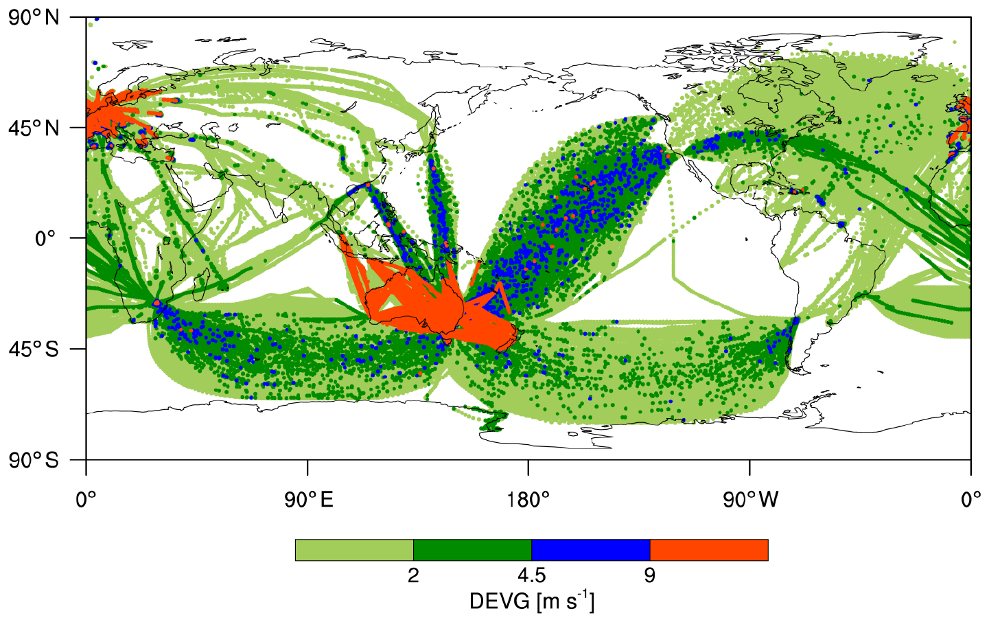
Figure 2 Horizontal locations of turbulence encounters expressed in raw DEVG values at altitudes above 15 kft (∼4.57 km) from October 2015 to September 2018.

Figure 3 shows the probability density functions (PDFs) of the raw DEVG values at altitudes above 15 kft (∼4.57 km) over the globe, the NH, and the SH for the same period (36 months). The primary peak falls within relatively small DEVG values (less than 8 m s⁻¹), and the secondary peak falls within relatively large DEVG values (greater than 8 m s⁻¹). This bimodal distribution, which is more prominent in the NH (blue curve) than in the SH (red curve), is highly suspicious considering that Kim et al. (2017) showed that the PDFs of the DEVG have a unimodal distribution following a lognormal distribution.

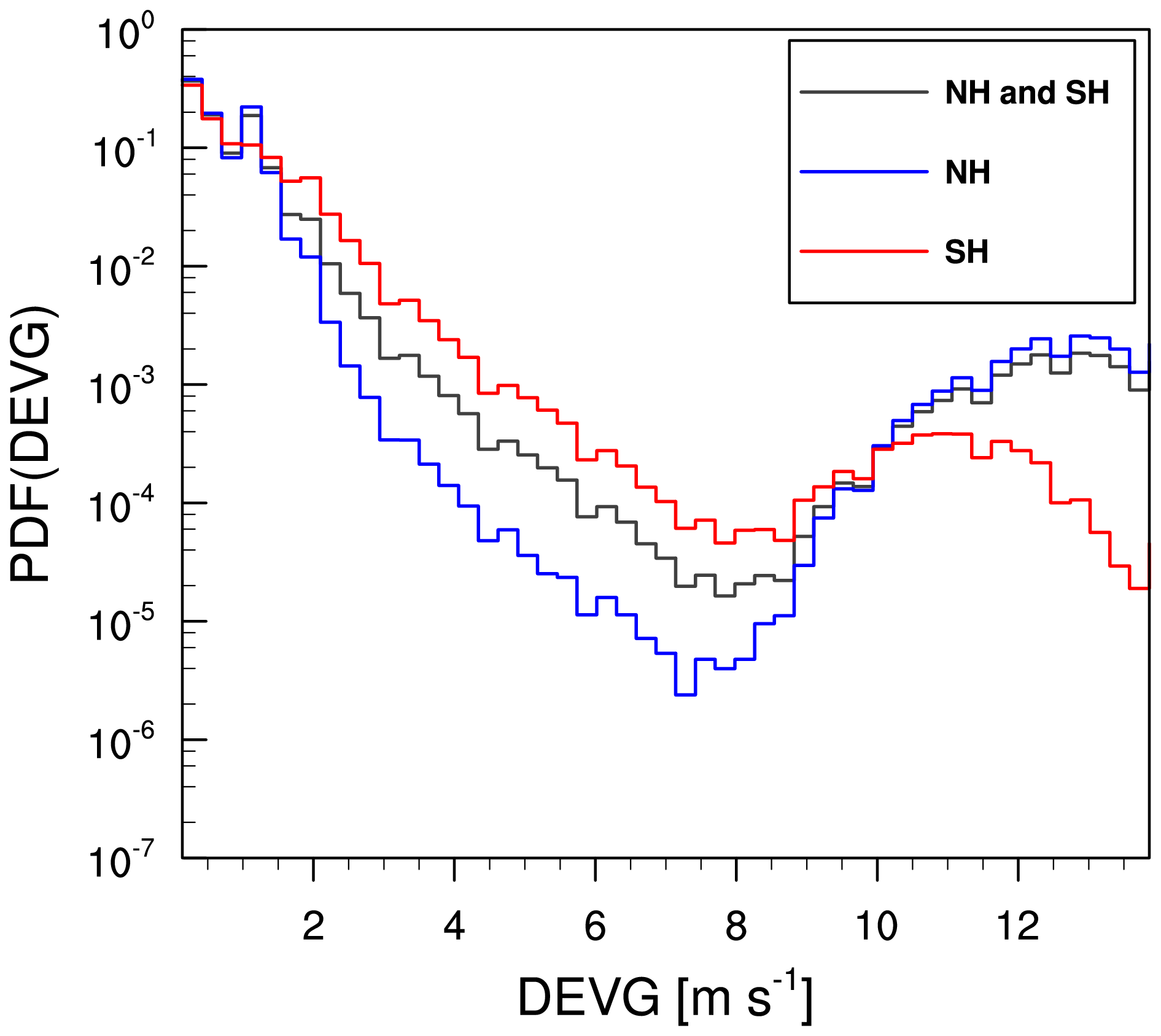
Figure 3 The probability density functions (PDFs) of the raw DEVG over the Northern Hemisphere (NH: blue line), the Southern Hemisphere (SH: red line), and the globe (NH and SH: black line) at altitudes above 15 kft (∼4.57 km) from October 2015 to September 2018.

To examine the regional PDFs of the raw DEVG, we choose the following eight regions: region 1 covers some of Europe, Africa, and Asia (8^∘ S–57^∘ N, 5–65^∘ E), region 2 covers East Asia (2–45^∘ N, 60–160^∘ E), region 3 covers the Pacific Ocean and North America (28^∘ S–50^∘ N, 70–178^∘ W), region 4 covers the North Atlantic Ocean (5–65^∘ N, 10–68^∘ W), region 5 covers the Indian Ocean (15–70^∘ S, 30–108^∘ E), region 6 covers Australia and New Zealand (0–45^∘ S, 110–180^∘ E), region 7 covers the South Pacific Ocean (30–75^∘ S, 70–178^∘ E), and region 8 covers the South Atlantic Ocean (42^∘ S–4^∘ N, 60^∘ W–28^∘ E).

Figure 4 shows the PDFs of the raw DEVG over these eight regions. As shown in Fig. 3, the PDFs of the DEVG in regions 1 and 6, covering Europe and Australia–New Zealand, respectively, show clear bimodal distributions. In contrast, the PDFs of the DEVG in regions 2–5 and 7–8 show the expected unimodal distributions. The DEVG in regions 4, 7, and 8 does not include strong turbulence events (e.g., DEVG >9 m s⁻¹). Figures 2–4 show that the raw DEVG reports may contain erroneous turbulence values, which requires QC procedures to remove.

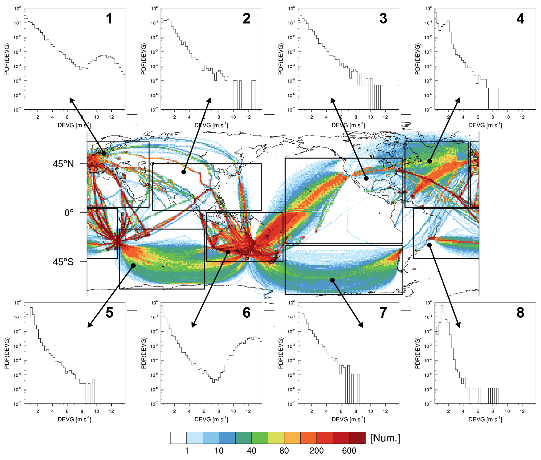
Figure 4 The PDFs of the raw DEVG over eight selected regions, which are indicated as rectangles in the global map, at altitudes above 15 kft (∼4.57 km) from October 2015 to September 2018. The eight regions are located in 8^∘ S–57^∘ N, 5–65^∘ E (region 1); 2–45^∘ N, 60–160^∘ E (region 2); 28^∘ S–50^∘ N, 70–178^∘ W (region 3); 5–65^∘ N, 10–68^∘ W (region 4); 15–70^∘ S, 30–108^∘ E (region 5); 0–45^∘ S, 110–180^∘ E (region 6); 30–75^∘ S, 70–178^∘ E (region 7); and 42^∘ S–4^∘ N, 60^∘ W–28^∘ E (region 8).

2.2 QC procedures

In the QC procedures, the DEVG, longitude, latitude, altitude, and flight tail number are used. Notably, aircraft-related information, such as aircraft type and tail number, is limited in the AMDAR dataset, and time series of basic variables required for a DEVG calculation are not available. Since the raw DEVG data with the same tail number sometimes include multiple flights, the flight tail number is only used to separate individual flights.

Figure 5 shows a flowchart of the QC procedures used, after some trial and error. First, the raw DEVG data are redistributed into an individual file which has the same flight tail number. Second, data are considered to be erroneous according to the following criteria:

1. if the number of observations in the individual file is less than eight;

2. if, for the individual file, more than two SEV and more than six MOD turbulence events are counted within the spatiotemporal window, which is defined as a circle with 100 km radius, a time window of ±1 h, and an altitude window of ±3 kft (∼0.91 km);

3. if there is only one reported SEV turbulence event, but no MOD turbulence event within a 200 km radius circle and time window of ±1 h;

4. if there is only one reported MOD turbulence event, but no LGT turbulence event within a 200 km radius circle and time window of ±1 h.

Applying these QC procedures, only the QC'd DEVG data (hereafter, QCDEVG) are examined in the present study.

Figure 5 The flowchart of quality control procedures.

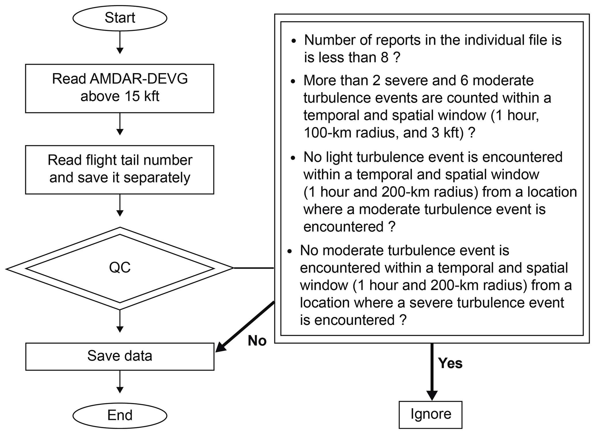
We adopt an approach that uses a cluster of the raw DEVG data within a certain spatiotemporal window to increase a confidence of a turbulence event, as the time series of recorded variables are not available. An early version of the QC procedures in the current study is designed, based on those by Gill (2014) and Meneguz et al. (2016), who used the global aircraft dataset. These QC procedures for the AMDAR data are revised based on active discussion with scientists and forecasters associated in the Aviation Weather Center (personal communications, from June to August 2018). The ratio of SEV to MOD turbulence events is larger in the current study (more than two out of six) than in other observational studies. For example, over South Korea, Kim and Chun (2011) showed 2.94 % MOD and 0.08 % SEV turbulence events from the PIREPs, while Kim and Chun (2016) showed 0.25 % (0.33 %) MOD and 0.04 % (0.04 %) SEV turbulence events from 1 min aircraft data over the globe (East Asia) and 5.1 % MOD and 0.34 % SEV turbulence events from the PIREPs over East Asia. Nevertheless, in the current study, the spatial and temporal windows are empirically determined to satisfactorily remove suspicious turbulence reports from the raw DEVG data. Considering that the raw DEVG data merged point samples from many kinds of flight over the globe, and time series of the DEVG and other recorded variables are not available, it is difficult to clearly identify the reason for suspicious DEVG values. Possible reasons for suspicious DEVG values could be power loss at the electrical contacts and a bug in the DEVG initialization logic, which is related to an intermittently added 1 g bias (Douglas Body, personal communication, 2019). A further investigation of the QC procedures of the DEVG remains for future work.

Figure 6 shows the horizontal locations of turbulence encounters according to the QCDEVG above 15 kft (∼4.57 km) for 36 months (from October 2015 to September 2018). The QC procedures indicate that 6 269 077 (97.28%) NIL, 170 199 (2.64 %) LGT, 5380 (0.083 %) MOD, and 32 (0.0005 %) SEV turbulence events defined by the DEVG values are valid. Most of the SEV turbulence events over Europe, Australia, and New Zealand are discarded by the QC procedures. Many discarded turbulence observations over Australia and New Zealand are due to continuous SEV turbulence reports or single SEV turbulence reports without consecutive NIL, LGT, and MOD turbulence events (not shown), while those over Europe are due to a single SEV or MOD turbulence report of the eight reports within an individual file. A relatively large number of SEV turbulence events over the Pacific Ocean and Indian Ocean pass the QC procedures and these are considered as valid turbulence reports. During the QC procedures, we checked horizontal distributions of the raw and QC'd DEVG data when all MOD and SEV turbulence events are reported. At least in the current study, the irrelevant turbulence events are discarded.

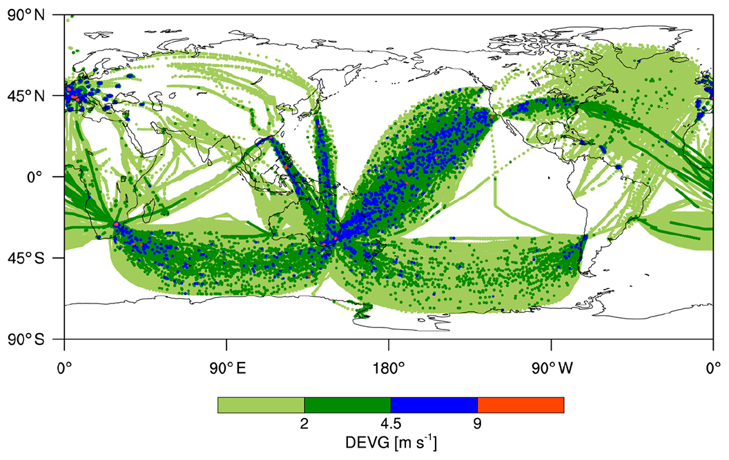
Figure 6 As in Fig. 2, except for the QCDEVG.

2.3 Spatial statistics of the QCDEVG

Figure 7 shows the PDFs of the QCDEVG at altitudes above 15 kft (∼4.57 km) over the globe, the NH, and the SH. As shown in Fig. 6, the secondary peaks in Fig. 3 are no longer apparent in Fig. 7. The SEV turbulence events defined by the DEVG values account for highly reduced percentages of 10⁻⁴ %. The PDFs of the QCDEVG indicate a unimodal distribution, which is consistent with Fig. 4 of Kim et al. (2017). The PDF for the NH indicates a relatively steep slope for low DEVG values compared with the PDF for the SH. Accordingly, the lognormal fitting, which will be shown in Sect. 3, is conducted for the NH and SH, separately, as characteristics of the QCDEVG are hemisphere dependent.

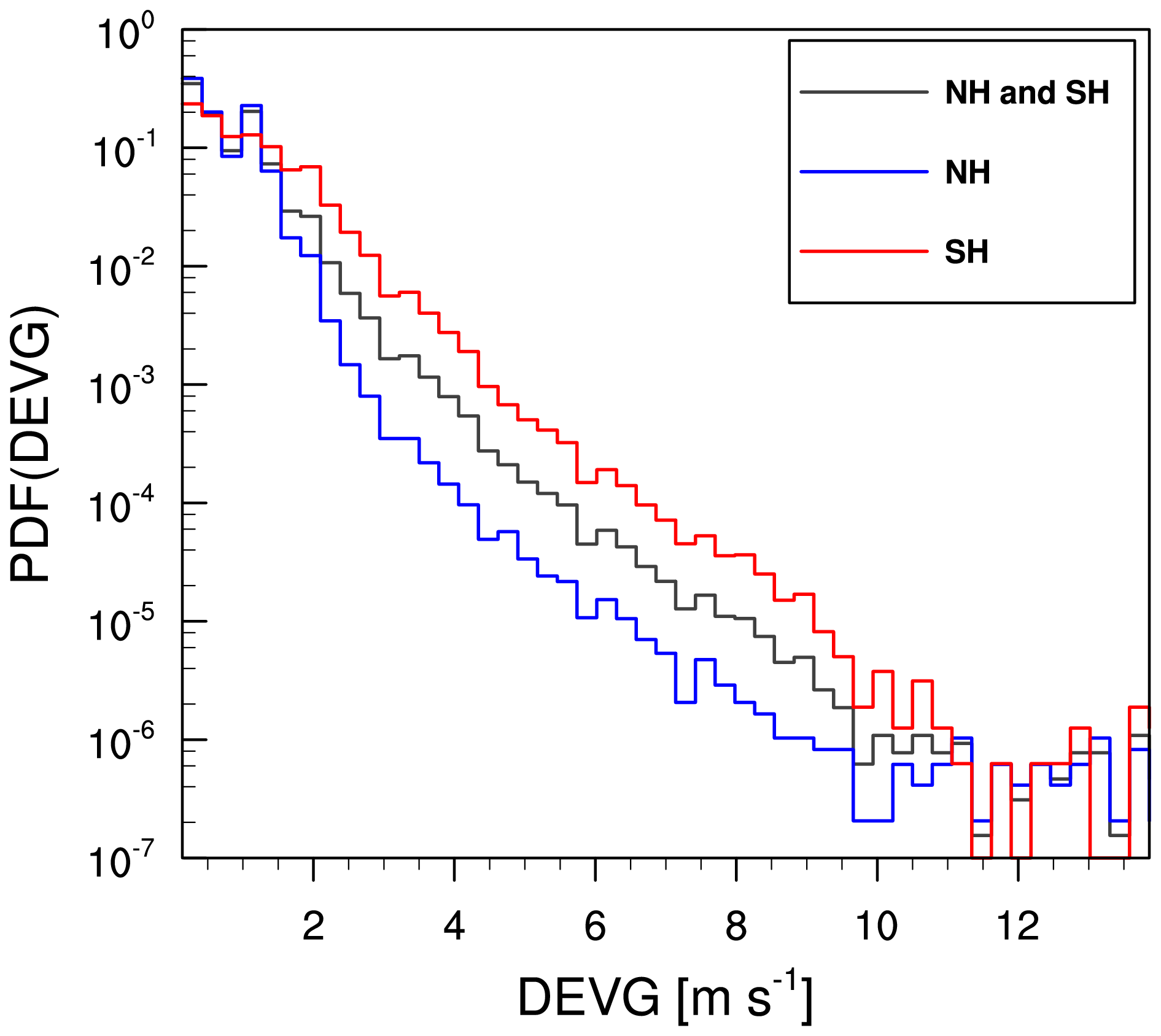
Figure 7 The PDFs of the QCDEVG over the globe (NH and SH: black line), NH (blue line), and SH (red line) at altitudes above 15 kft (∼4.57 km) from October 2015 to September 2018.

Figure 8 shows the regional PDFs of the QCDEVG values over the eight regions shown in Fig. 4. The horizontal distribution of the number of the QCDEVG data accumulated within the $\mathrm{1}{}^{\circ }\times \mathrm{1}{}^{\circ }$ horizontal grid box is also indicated in Fig. 8. Most DEVG reports are in the SH and along the narrow flight tracks over the Atlantic Ocean and between Africa and Europe or Asia. The PDFs of the QCDEVG archived in regions 1 and 6 show unimodal distributions. The PDFs of the QCDEVG show quite similar distributions to those calculated using the raw DEVG for the six regions (regions 2–5 and 7–8). The QCDEVG data in regions 5–8 generally are concentrated in the low DEVG value compared with those in regions 1–4. Our focus is to remove suspicious turbulence reports within the limited aircraft-related information and to obtain a reasonable PDF indicating a unimodal distribution. In this regard, the quality of the QCDEVG is considered adequate for the EDR conversion.

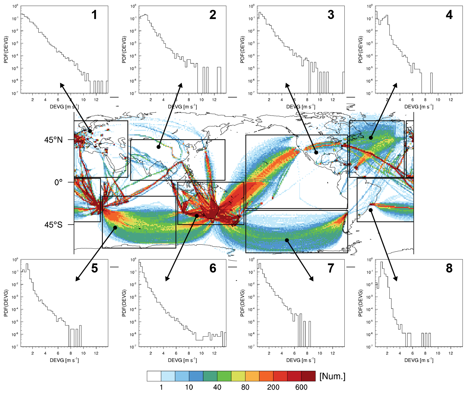
Figure 8 Horizontal distribution of the number of the QCDEVG data at altitudes above 15 kft (∼4.57 km), accumulated within a $\mathrm{1}{}^{\circ }\times \mathrm{1}{}^{\circ }$ horizontal grid box from October 2015 to September 2018. The PDFs of the QCDEVG over eight selected regions, superimposed on the global map by rectangles.

3 Conversion of the QCDEVG to the EDR

The QCDEVG is converted to the EDR using two methods (hereafter, DEVG-derived EDR), as EDR is the preferred turbulence metric. The methods considered in the current study are based on Sharman and Pearson (2017) and Kim et al. (2017). Brief descriptions of the two methods are provided below.

3.1 EDR conversion using the lognormal mapping scheme

Considering that the distribution of observed EDR in the free atmosphere approximately follows a lognormal distribution (Nastrom and Gage, 1985; Frehlich, 1992; Cho et al., 2003; Frehlich and Sharman, 2004; Sharman et al., 2014; Kim et al., 2017), Sharman and Pearson (2017) proposed a statistical mapping equation applying NWP-based turbulence diagnostics to the EDR. Assuming a lognormal property for turbulence forecasting diagnostics, the simplest mapping between a raw turbulence diagnostic D and the EDR is provided by

$$\begin{array}{}\text{(4)}& \text{ln}\left(D^{*}\right)=\ln \left(\mathrm{EDR}\right)=a+b\ln \left(D\right),\end{array}$$

where D^* is the remapped EDR value corresponding to the raw turbulence diagnostic D, slope b is the ratio between the standard deviation (SD) of ln(EDR) and SD of ln($D\left)\right[b=\text{SDln}\left(\text{EDR}\right)/\text{SDln}\left(D\right)=C_{\mathrm{2}}/\text{SDln}\left(D\right)]$, and the intercept a is the difference between the mean of ln(EDR) and mean of $\text{ln}\left(D\right)[a=\langle \text{ln}(\text{EDR})\rangle -b\langle \text{ln}(D)\rangle =C_{\mathrm{1}}-b\langle \text{ln}(D)\rangle$, where the angle brackets indicate the ensemble mean]. Here, C₁ and C₂ are the climatological values of the mean and SD of ln(EDR), respectively, which are obtained from the lognormal fits to the EDR estimates of in situ equipped aircraft from 2009 to 2014. It is noted that C₁ and C₂ may be different in different regions.

To utilize this statistical mapping equation to obtain the DEVG-derived EDRs, the turbulence diagnostic D is replaced with the DEVG value. Thus, Eq. (4) can be written as

$$\begin{array}{}\text{(5)}& \text{ln}\left({\text{DEVG}}^{*}\right)=\ln \left(\text{EDR}\right)=a+b\ln \text{(DEVG)},\end{array}$$

where DEVG^* is the remapped EDR value corresponding to the QCDEVG value. The intercept a and the slope b can be written as

$$\begin{array}{}\text{(6)}& \begin{array}{rl}& a=\langle \text{ln(EDR)}\rangle -b\langle \text{ln(DEVG)}\rangle =C_{\mathrm{1}}-b\langle \text{ln(DEVG)}\rangle \\ & \text{and}\\ & b=\text{SDln(EDR)}/\text{SDln(DEVG)}=C_{\mathrm{2}}/\text{SDln(DEVG)}.\end{array}\end{array}$$

The parameters C₁ and C₂ for four different altitude bands (−2.248 and 0.4235 for altitudes of 0–10 kft (0–∼3.05 km), −2.578 and 0.557 for altitudes of 10–20 kft (∼3.05–6.1 km), −2.953 and 0.602 for altitudes of 20–45 kft (∼6.1–13.72 km), and −2.572 and 0.5067 for altitudes above 0 ft, respectively) are given in Sharman and Pearson (2017). The parameters C₁ and C₂ for the 20–45 kft (∼6.1–13.72 km) altitude band (−2.953 and 0.602, respectively) are utilized in the current study. To obtain the mean and SD of ln(DEVG), the values of the QCDEVG over the NH and SH are calculated from the lognormal fitting via the optimization function “fminsearch” in the MATLAB package (Lagarias et al., 1998; see also https://www.mathworks.com/help/matlab/ref/fminsearch.html, last access: 23 March 2020). The EDR converted from this method is called EDR-SP17, hereafter.

Figure 9 shows the lognormal fits (curves) applied to the PDFs (circles) of the QCDEVG values over the NH and SH (red and blue lines in Fig. 7, respectively). To obtain an optimized lognormal curve, some of the highest and lowest bins (open circles) of the QC DEVG are not used for the lognormal fits. At the highest bins, there are not enough data for reliable lognormal fits, while at the lowest bins, instrument noise may be affecting the result and the small QCDEVG values corresponding to nonturbulent conditions are not of practical interest. The mean values of ln(DEVG) over the NH and SH are −0.69926 and −1.4397 m s⁻¹, respectively, and the SDs of ln(DEVG) over the NH and SH are 0.6956 and 0.7773 m s⁻¹, respectively. The mean and SD of ln(DEVG) over the SH and NH are used for the EDR conversion (EDR-SP17). When the PDFs of the QCDEVG over different conditions (over land and ocean, different altitude ranges (15–25, 25–35, and 35 kft), seasons (spring, summer, autumn, and winter), times (day and night), and different latitude bands with a spacing of 20^∘) are computed, the mean and SD of ln(DEVG) are not significantly changed for the aforementioned conditions, except that those in latitudes equatorward of 30^∘ are clearly smaller than those poleward of 30^∘ (not shown).

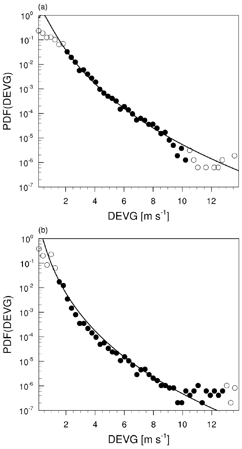
Figure 9 The PDFs (circles) of the QCDEVG and lognormal fit (continuous line) over the QCDEVG over the (a) NH and (b) SH. The filled circles indicate data that were used in the fit, and the open circles indicate data that are excluded from the fit.

3.2 EDR conversion using the prescribed best-fit function

Kim et al. (2017) investigated two turbulence indicators (the EDR and the DEVG) calculated by the algorithms using the time series of several variables recorded by Hong Kong-based airline flight data recorders for 39 months from February 2011 to April 2014. On a one-to-one basis, relationships between the EDR and DEVG are calculated for three different Boeing (B) aircraft models (B747-400, B777-200, and B777-300) and three different Airbus (A) aircraft models (A320-200, A321-200, and A330-300), based on the best-fit quadratic functions for Boeing and Airbus aircraft, separately.

The quadratic equations for the Boeing and Airbus aircraft data are as follows:

$$\begin{array}{}\text{(7)}& {\displaystyle }\begin{array}{rl}{\mathrm{DEVG}}^{*}& =\text{EDR}=\mathrm{0.0031}\left({\mathrm{DEVG}}^{\mathrm{2}}\right)+\mathrm{0.0286}\left(\mathrm{DEVG}\right)\\ & +\mathrm{0.0114},\text{for Boeing}\end{array}\text{(8)}& {\displaystyle }\begin{array}{rl}{\mathrm{DEVG}}^{*}& =\text{EDR}=\mathrm{0.003}\left({\mathrm{DEVG}}^{\mathrm{2}}\right)+\mathrm{0.0324}\left(\mathrm{DEVG}\right)\\ & +\mathrm{0.0516},\text{for Airbus},\end{array}\end{array}$$

where DEVG^* is the converted EDR corresponding to the QCDEVG. Although two different DEVG-derived EDRs can be derived using the above two quadratic equations, the DEVG-derived EDR obtained from the quadratic equation for the Boeing aircraft (Eq. 7), which shows a high correlation between the EDR and DEVG, is only considered in the current study. The EDR converted from this method is called for EDR-KCC17, hereafter.

3.3 Spatial statistics of the DEVG-derived EDRs

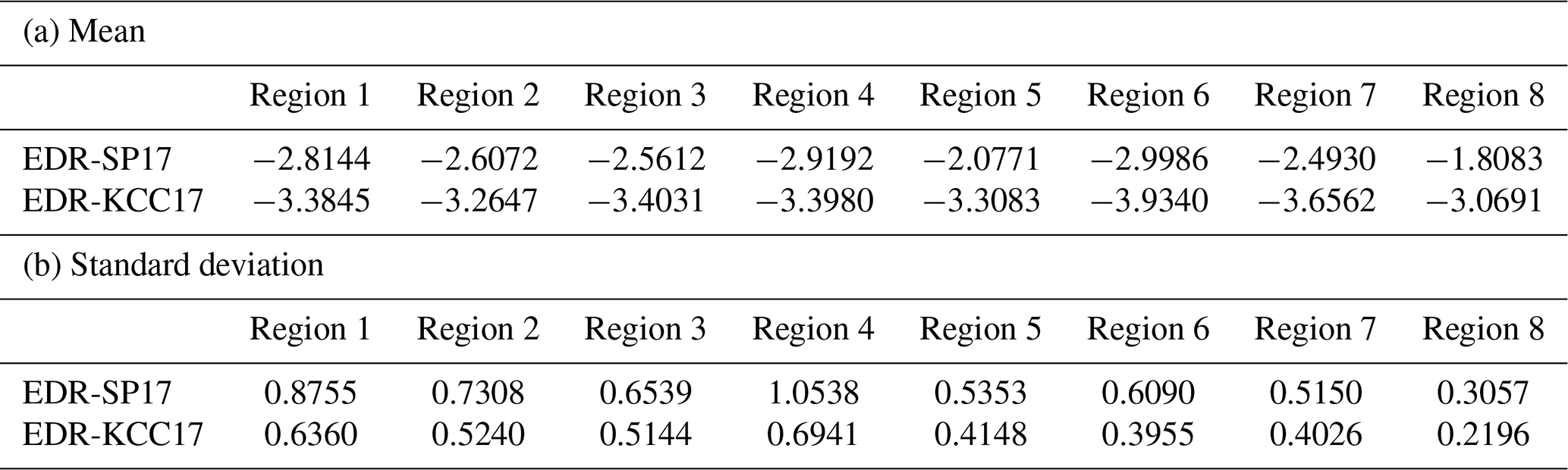
Table 1 shows the mean and SD of the natural logarithms of EDR-SP17 and EDR-KCC17, ln(EDR-SP17) and ln(EDR-KCC17), respectively, for the eight regions indicated by rectangles in Fig. 8. The mean and SD of the resultant DEVG-derived EDRs differ slightly among the eight specified regions. Nevertheless, regarding the mean of the natural logarithm of the EDR, EDR-SP17 (from −2.9986 to −1.8083 m^2∕3 s⁻¹) is larger than EDR-KCC17 (from −3.9340 to −3.0691 m^2∕3 s⁻¹) for all eight regions, with differences in magnitude ranging from 0.4788 to 1.2608 m^2∕3 s⁻¹. For the SD of the natural logarithm of the EDR, EDR-SP17 (from 0.3057 to 1.0538 m^2∕3 s⁻¹) is larger than EDR-KCC17 (from 0.2196 to 0.6941 m^2∕3 s⁻¹) for all eight regions, with differences in magnitude ranging from 0.0861 to 0.3597 m^2∕3 s⁻¹.

Table 1 Values of the mean and standard deviation (SD) of the natural logarithms of EDR-SP17 and EDR-KCC17, over the eight selected regions indicated in Fig. 8, from October 2015 to September 2018. The unit is m^2∕3 s⁻¹. Note that EDR-SP17 and EDR-KCC17 are the DEVG-derived EDRs obtained using the methods of Sharman and Pearson (2017) and Kim et al. (2017), respectively.

Given that EDR-SP17 and EDR-KCC17 have different characteristics, validation of the two different methods is required. Accordingly, the EDRs estimated from in situ equipped aircraft implemented in some United States (US) commercial aircraft (Sharman et al., 2014; Cornman, 2016) are used as the reference data (hereafter, USEDR). The comparison between the USEDR and DEVG-derived EDRs proposed in the current study for the same period (from October 2015 to September 2018) is conducted by comparing the mean and SD values of the natural logarithms of three different EDRs (EDR-SP17, EDR-KCC17, and USEDR) for the specified regions.

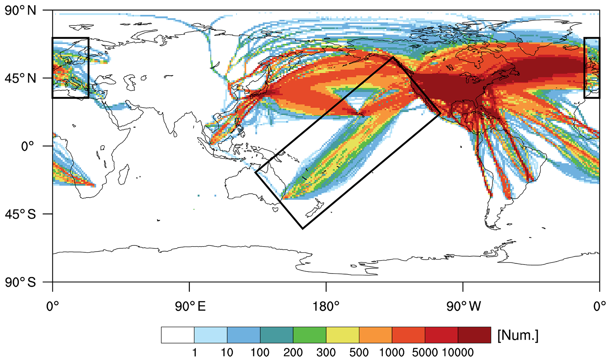
Figure 10 Horizontal distribution of the number of USEDR data at altitudes above 15 kft (∼4.57 km), accumulated within a $\mathrm{1}{}^{\circ }\times \mathrm{1}{}^{\circ }$ horizontal grid box from October 2015 to September 2018. The regions of Europe and the Pacific Ocean are indicated by rectangles.

Figure 11 The PDFs of EDR-SP17 (black line), EDR-KCC17 (blue line), and USEDR (red line) at altitudes above 15 kft (∼4.57 km) from October 2015 to September 2018 over (a) Europe and (b) the Pacific Ocean routes indicated in Fig. 10.

Figure 10 shows the horizontal distribution of the USEDR counts (reference data) at altitudes above 15 kft (∼4.57 km) accumulated within a $\mathrm{1}{}^{\circ }\times \mathrm{1}{}^{\circ }$ horizontal grid box from the same period (36 months) as the DEVG data. Compared with Fig. 8, the USEDR data mainly cover large portions of the NH, which include the flight routes of the Pacific Ocean, North and South America, the Atlantic Ocean, and Europe. To evaluate the feasibility of deriving the EDRs from the DEVG using the two methods (EDR-SP17 and EDR-KCC17), the mean and SD of three different EDRs are calculated over the two specified regions represented by the rectangles in Fig. 10; one region covers some of Europe and the other covers the Pacific Ocean, which includes flight routes between North America and Australia. Although there is a large amount of USEDR data (Fig. 10) over North America and the Atlantic Ocean, unfortunately, the DEVG data (Fig. 8) over these two regions are insufficient for further analysis.

Figure 11 shows the PDFs of EDR-SP17, EDR-KCC17, and USEDR data over the two rectangles in Fig. 10 from October 2015 to September 2018. Over both Europe and the Pacific Ocean, the distributions of the PDF of EDR-SP17 and USEDR are similar. Especially for the Pacific Ocean region, the PDFs of EDR-SP17 and USEDR at values larger than ∼0.22 m^2∕3 s⁻¹ are in very good agreement. Over Europe (Fig. 11a), the values of EDR-SP17 are generally larger than those of EDR-KCC17 and USEDR, while over the Pacific Ocean (Fig. 11b), EDR-SP17 and USEDR are similar. The EDR-KCC17 has a larger percentage of low EDR values (≲0.1 m^2∕3 s⁻¹) compared to EDR-SP17 and USEDR in the two regions. For each PDF shown in Fig. 11, the root mean square error (RMSE) of the occurrence frequency of two different EDRs (EDR-SP17 and EDR-KCC17) is calculated with respect to that of the USEDR. Over Europe, the RMSE of EDR-SP17 is 0.0157, and that of EDR-KCC17 is 0.0441. Over the Pacific Ocean, the RMSE of EDR-SP17 is 0.0504, and that of EDR-KCC17 is 0.0903, implying that the occurrence frequency of EDR-SP17 is relatively close to that of the USEDR. The PDFs of EDR-SP17 and USEDR generally follow lognormal distributions, whereas the PDF of EDR-KCC17 departs somewhat from a lognormal distribution especially at low EDR values (≲0.14 m^2∕3 s⁻¹) (not shown). It is noted that the slight difference between the EDR calculations of Cornman (2016) and Haverdings and Chan (2010) might result in the observed difference in the EDR statistics and affect the DEVG-derived EDRs.

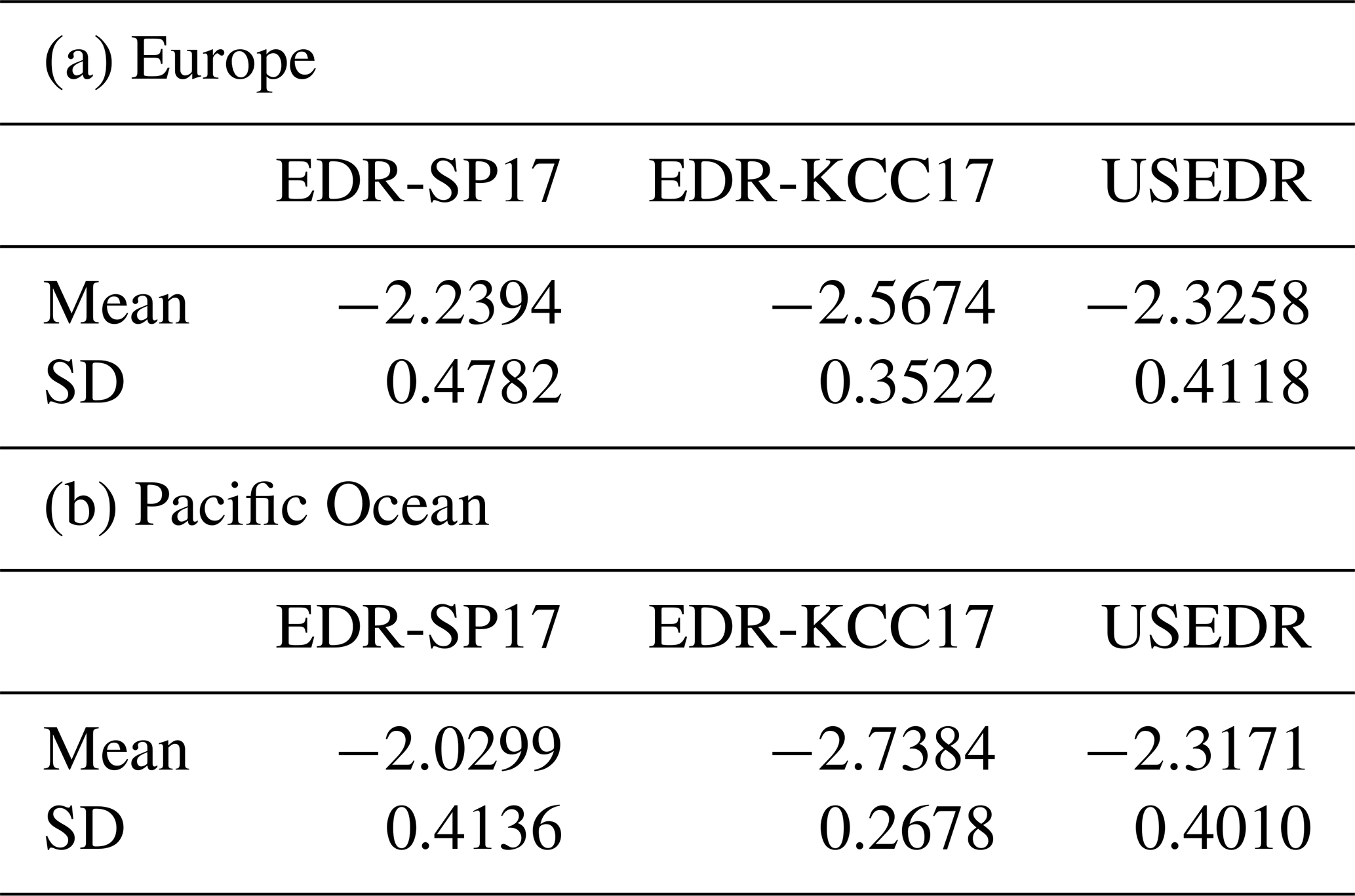
Table 2 shows the mean and SD of the natural logarithm of three different EDRs (EDR-SP17, EDR-KCC17, and USEDR) over Europe and the Pacific Ocean. For the region of Europe, the mean values of ln(EDR-SP17) and ln(EDR-KCC17) are −2.2394 and −2.5674 m^2∕3 s⁻¹, respectively, and the SDs of ln(EDR-SP17) and ln(EDR-KCC17) are 0.4782 and 0.3522 m^2∕3 s⁻¹, respectively. For the Pacific Ocean region, the mean values of ln(EDR-SP17) and ln(EDR-KCC17) are −2.0299 and −2.7384 m^2∕3 s⁻¹, respectively, and the SDs of ln(EDR-SP17) and ln(EDR-KCC17) are 0.4136 and 0.2678 m^2∕3 s⁻¹, respectively. EDR-SP17 and USEDR generally have relatively close mean and SD values, which implies that the EDR-SP17 technique is more accurate at least in the current case. In our current limited study, the statistical properties between EDR-SP17 and USEDR appear slightly different, with higher intensities overall over Europe than the Pacific Ocean. However, because the results are considered only over two regions, further evaluation of the two different methods for deriving EDRs from DEVG is required over different regions and longer period datasets.

Table 2 Values of the mean and SD of the natural logarithms of EDR-SP17, EDR-KCC17, and USEDR over (a) Europe and (b) the Pacific Ocean routes indicated in Fig. 10, from October 2015 to September 2018. The unit is m^2∕3 s⁻¹.

4 Summary and discussion

In the current study, we convert the AMDAR-provided turbulence indicator, the DEVG, to the EDR to obtain quantitative and consistent turbulence observations globally. We use the DEVG data archived in the NOAA AMDAR (raw DEVG) data for 36 months (October 2015 to September 2018). In the raw DEVG data, there are many suspicious strong-intensity-turbulence reports that cause bimodal distributions in the PDFs of the DEVG. To remove erroneous turbulence reports in the raw DEVG data, QC procedures are developed by applying optimally determined thresholds to the raw DEVG dataset. The QC'd DEVG values are converted to the EDR, which is the ICAO standard turbulence intensity metric. The conversion of the DEVG to the EDR is conducted using two methods. Sharman and Pearson (2017) proposed a linear mapping equation assuming a lognormal property for raw turbulence diagnostics, while Kim et al. (2017) proposed a best-fit curve (quadratic equation) between the EDR and DEVG, based on a one-to-one comparison between the EDR and DEVG calculated using the same flight data. The PDFs of the resultant DEVG-derived EDRs from the two methods, referred to as EDR-SP17 and EDR-KCC17, are compared with those of the USEDR for the two regions covering Europe and the Pacific Ocean. It is found that EDR-SP17 has a relatively similar distribution with the USEDR at least for the current case.

A robust conversion of the DEVG to the EDR would improve the verification of turbulence forecasts globally and the investigation of global characteristics of aviation turbulence, as the USEDR data are still of limited availability globally (Fig. 10). Indeed, the characteristics of aviation turbulence over the NH have been investigated in many previous studies, while those over the SH have not, in part due to a lack of observational data. In this regard, qualified DEVG-derived EDRs can be an important additional source of information globally, especially in most of the SH. Additionally, the DEVG data used in the current study can represent valuable observations for the evaluation of turbulence diagnostics related to convection (Kim et al., 2019), given that the DEVG data contain substantial turbulent information over the tropical region. Together with the existing the USEDR data over the NH, the DEVG-derived EDRs in the SH and tropical regions can be merged into a homogenized global turbulence dataset, which will contribute to improvement of global aviation turbulence forecasting as well as to construction of a global climatology of upper-level turbulence.