the Creative Commons Attribution 4.0 License.
the Creative Commons Attribution 4.0 License.
 | 07 Apr 2020
Evaluation and calibration of a low-cost particle sensor in ambient conditions using machine-learning methods
Minxing Si
Ying Xiong
Particle sensing technology has shown great potential for monitoring particulate matter (PM) with very few temporal and spatial restrictions because of its low cost, compact size, and easy operation. However, the performance of low-cost sensors for PM monitoring in ambient conditions has not been thoroughly evaluated. Monitoring results by low-cost sensors are often questionable. In this study, a low-cost fine particle monitor (Plantower PMS 5003) was colocated with a reference instrument, the Synchronized Hybrid Ambient Real-time Particulate (SHARP) monitor, at the Calgary Varsity air monitoring station from December 2018 to April 2019. The study evaluated the performance of this low-cost PM sensor in ambient conditions and calibrated its readings using simple linear regression (SLR), multiple linear regression (MLR), and two more powerful machine-learning algorithms using random search techniques for the best model architectures. The two machine-learning algorithms are XGBoost and a feedforward neural network (NN). Field evaluation showed that the Pearson correlation (r) between the low-cost sensor and the SHARP instrument was 0.78. The Fligner and Killeen (F–K) test indicated a statistically significant difference between the variances of the PM2.5 values by the low-cost sensor and the SHARP instrument. Large overestimations by the low-cost sensor before calibration were observed in the field and were believed to be caused by the variation of ambient relative humidity. The root mean square error (RMSE) was 9.93 when comparing the low-cost sensor with the SHARP instrument. The calibration by the feedforward NN had the smallest RMSE of 3.91 in the test dataset compared to the calibrations by SLR (4.91), MLR (4.65), and XGBoost (4.19). After calibrations, the F–K test using the test dataset showed that the variances of the PM2.5 values by the NN, XGBoost, and the reference method were not statistically significantly different. From this study, we conclude that a feedforward NN is a promising method to address the poor performance of low-cost sensors for PM2.5 monitoring. In addition, the random search method for hyperparameters was demonstrated to be an efficient approach for selecting the best model structure.
- Article
(8870 KB) - Full-text XML
- BibTeX
- EndNote


Particulate matter (PM), whether it is natural or anthropogenic, has pronounced effects on human health, visibility, and global climate (Charlson et al., 1992; Seinfeld and Pandis, 1998). To minimize the harmful effects of PM pollution, the Government of Canada launched the National Air Pollution Surveillance (NAPS) program in 1969 to monitor and regulate PM and other criteria air pollutants in populated regions, including ozone (O3), sulfur dioxide (SO2), carbon monoxide (CO), and nitrogen dioxide (NO2). Currently, PM monitoring is routinely carried out at 286 designated air sampling stations in 203 communities in all provinces and territories of Canada (Government of Canada, 2019). Many of the monitoring stations use a beta attenuation monitor (BAM), which is based on the adsorption of beta radiation, or a tapered element oscillating microbalance (TEOM) instrument, which is a mass-based technology to measure PM concentrations. An instrument that combines two or more technologies, such as the Synchronized Hybrid Ambient Real-time Particulate (SHARP) monitor, is also used in some monitoring stations. The SHARP instrument combines light scattering with beta attenuation technologies to determine PM concentrations.
Although these instruments are believed to be accurate for measuring PM concentration and have been widely used by many air monitoring stations worldwide (Chow and Watson, 1998; Patashnick and Rupprecht, 1991), they have common drawbacks: they can be challenging to operate, bulky, and expensive. The instrument costs from CAD 8000 (Canadian dollars) to tens of thousands of dollars (Chong and Kumar, 2003). The SHARP instrument used in this study as a reference method costs approximately CAD 40 000 (CD Nova Instruments Ltd., 2017). Significant resources, such as specialized personnel and technicians, are also required for regular system calibration and maintenance. In addition, the sparsely spread stations may only represent PM levels in limited areas near the stations because PM concentrations vary spatially and temporally depending on local emission sources as well as meteorological conditions (Xiong et al., 2017). Such a low-resolution PM monitoring network cannot support public exposure and health effects studies that are related to PM because these studies require high-spatial- and temporal-resolution monitoring networks in the community (Snyder et al., 2013). In addition, the well-characterized scientific PM monitors are not portable due to their large size and volumetric flow rate, which means they are not practical for measuring personal PM exposure (White et al., 2012).
As a possible solution to the above problems, a large number of low-cost PM sensors could be deployed, and a high-resolution PM monitoring network could be constructed. Low-cost PM sensors are portable and commercially available. They are cost-effective and easy to deploy, operate, and maintain, which offers significant advantages compared to conventional analytical instruments. If many low-cost sensors are deployed, PM concentrations can be monitored continuously and simultaneously at multiple locations for a reasonable cost (Holstius et al., 2014). A dense monitoring network using low-cost sensors can also assist in mapping hot spots of air pollution, creating emission inventories of air pollutants, and estimating adverse health effects due to personal exposure to PM (Kumar et al., 2015).
However, low-cost sensors present challenges for broad application and installation. Most sensor systems have not been thoroughly evaluated (Williams et al., 2014), and the data generated by these sensors are of questionable quality (Wang et al., 2015). Currently, most low-cost sensors are based on laser light-scattering (LLS) technology, and the accuracy of LLS is mostly affected by particle composition, size distribution, shape, temperature, and relative humidity (Jayaratne et al., 2018; Wang et al., 2015).
Several studies have evaluated LLS sensors by comparing the performance of low-cost sensors with medium- to high-cost instruments under laboratory and ambient conditions. For example, Zikova et al. (2017) used low-cost Speck monitors to measure PM2.5 concentrations in indoor and outdoor environments, and the low-cost sensors overestimated the concentration by 200 % for indoor and 500 % for outdoor compared to a reference instrument – the Grimm 1.109 dust monitor. Jayaratne et al. (2018) reported that PM10 concentrations generated by a Plantower low-cost particle sensor (PMS 1003) were 46 % greater than a TSI 8350 DustTrak DRX aerosol monitor under a foggy environment. Wang et al. (2015) compared PM measurements from three low-cost LLS sensors – Shinyei PPD42NS, Samyoung DSM501A, and Sharp GP2Y1010AU0F – with a SidePack (TSI Inc.) using smoke from burning incense. High linearity was found with R2 greater than 0.89, but the responses depended on particle composition, size, and humidity. The Air Quality Sensor Performance Evaluation Center (AQ-SPEC) of the South Coast Air Quality Management District (SCAQMD) also evaluated the performances of three Purple Air PA-II sensors (model: Plantower PMS 5003) by comparing their readings with two United States Environmental Protection Agency (US EPA) Federal Equivalent Method (FEM) instruments – BAM (MetOne) and Grimm dust monitors in laboratory and field environments in southern California (Papapostolou et al., 2017). Overall, the three sensors showed moderate to good accuracy compared to the reference instrument for PM2.5 for a concentration range between 0 and 250 µg m−3. Lewis et al. (2016) evaluated low-cost sensors in the field for O3, nitrogen oxide (NO), NO2, volatile organic compounds (VOCs), PM2.5, and PM10; only the O3 sensors showed good performance compared to the reference measurements.
Several studies have developed calibration models using multiple techniques to improve low-cost sensor performance. For example, De Vito et al. (2008) tested feedforward neural network (NN) calibration for benzene monitoring and reported that further calibration was needed for low concentrations. Bayesian optimization was also used to search feedforward NN structures for the calibrations of CO, NO2, and NOx low-cost sensors (De Vito et al., 2009). Zheng et al. (2018) calibrated the Plantower low-cost particle sensor PMS 3003 by fitting a linear least-squares regression model. A nonlinear response was observed when ambient PM2.5 exceeded 125 µg m−3. The study concluded that a quadratic fit was more appropriate than a linear model to capture this nonlinearity.
Zimmerman et al. (2018) explored three different calibration models, including laboratory univariate linear regression, empirical MLR, and a more modern machine-learning algorithm, random forests (RF), to improve the Real-time Affordable Multiple-Pollutant (RAMP) sensor's performance. They found that the sensors calibrated by RF models showed improved accuracy and precision over time, with average relative errors of 14 % for CO, 2 % for CO2, 29 % for NO2, and 15 % for O3. The study concluded that combing RF models with low-cost sensors is a promising approach to address the poor performance of low-cost air quality sensors.
Spinelle et al. (2015) reported several calibration methods for low-cost O3 and NO2 sensors. The best calibration method for NO2 was an NN algorithm with feedforward architecture. O3 could be calibrated by simple linear regression (SLR). Spinelle et al. (2017) also evaluated and calibrated NO, CO, and CO2 sensors, and the calibrations by feedforward NN architectures showed the best results. Similarly, Cordero et al. (2018) performed a two-step calibration for an AQmesh NO2 sensor using supervised machine-learning regression algorithms, including NNs, RFs, and support vector machines (SVMs). The first step produced an explanatory variable using multivariate linear regression. In the second step, the explanatory variable was fed into machine-learning algorithms, including RF, SVM, and NN. After the calibration, the AQmesh NO2 sensor met the standards of accuracy for high concentrations of NO2 in the European Union's Directive 2008/50/EC on air quality. The results highlighted the need to develop an advanced calibration model, especially for each sensor, as the responses of individual sensors are unique.
Williams et al. (2014) evaluated eight low-cost PM sensors; the study showed frequent disagreement between the low-cost PM sensors and FEMs. In addition, the study concluded that the performances of the low-cost sensors were significantly impacted by temperature and relative humidity (RH). Recurrent NN architectures were also tested for calibrating some gas sensors (De Vito et al., 2018; Esposito et al., 2016). The results showed that the dynamic approaches performed better than traditional static calibration approaches. Calibrations of PM2.5 sensors were also reported in recent studies. Lin et al. (2018) performed two-step calibrations for PM2.5 sensors using 236 hourly data points collected on buses and road-cleaning vehicles. The first step was to construct a linear model, and the second step used RF machine learning for further calibration. The RMSE after the calibrations was 14.76 µg m−3 compared to a reference method. The reference method used in this study was a Dylos DCI1700 device, which is not a US EPA federal reference method (FRM) or FEM. Loh and Choi (2019) trained and tested the SVM, K-nearest neighbor, RF, and XGBoost machine-learning algorithms to calibrate PM2.5 sensors using 319 hourly data points. XGBoost archived the best performance with an RMSE of 5.0 µg m−3. However, the low-cost sensors in this study were not colocated with the reference method, and the machine-learning models were not tested using unseen data (test data) for predictive power and overfitting.
Although there have been studies on calibrating low-cost sensors, most of them focused on gas sensors or used short-term data to calibrate PM sensors. To our best knowledge, no one has reported studies on PM sensor calibration using random search techniques for the best machine-learning model configuration under ambient conditions during different seasons. In this study, a low-cost fine particle monitor (Plantower PMS 5003) was colocated with a SHARP monitor model 5030 at Calgary Varsity air monitoring station in an outdoor environment from 7 December 2018 to 26 April 2019. The SHARP instrument is the reference method in this study and is a US EPA FEM (US EPA, 2016). The objectives of this study are (1) to evaluate the performance of the low-cost PM sensor in a range of outdoor environmental conditions by comparing its PM2.5 readings with those obtained from the SHARP instrument and (2) to assess four calibration methods: (a) an SLR or univariate linear regression based on the low-cost sensor values; (b) a multiple linear regression (MLR) using the PM2.5, RH, and temperature measured by the low-cost sensor as predictors; (c) a decision-tree-based ensemble algorithm, called XGBoost or Extreme Gradient Boosting; and (d) a feedforward NN architecture with a back-propagation algorithm.
XGBoost and NN are the most popular algorithms used on Kaggle – a platform for data science and machine-learning competition. In 2015, 17 winners in 29 competitions on Kaggle used XGBoost, and 11 winners used deep NN algorithms (Chen and Guestrin, 2016).
This study is unique in the following ways.
-
To the best of our knowledge, this is the first comprehensive study using long-term data to calibrate low-cost particle sensors in the field. Most previous studies focused on calibrating gas sensors (Maag et al., 2018). There are two studies on PM sensor calibrations using machine learning, but they used a short-term dataset that did not include seasonal changes in ambient conditions (Lin et al., 2018; Loh and Choi, 2019). The shortcomings of the two studies were discussed above.
-
Although several studies have researched the calibration of gas sensors using NN, this study explores multiple hyperparameters to search for the best NN architecture. Previous research configured one to three hyperparameters compared to six in this study (De Vito et al., 2008, 2009, 2018; Esposito et al., 2016; Spinelle et al., 2015, 2017). In addition, this study tested the rectified linear unit (ReLU) as the activation function in the feedforward NN. Compared to the sigmoid and tanh activation functions used in previous studies for NN calibration models, the ReLU function can accelerate the convergence of stochastic gradient descent to a factor of 6 (Krizhevsky et al., 2017).
-
Previous NN and tree-based calibration models used a manual search or grid search for hyperparameter tuning. This study introduced a random search method for the best calibration models. A random search is more efficient than a traditional manual and grid search (Bergstra and Bengio, 2012) and evaluates more of the search space, especially when the search space is more than three dimensions (Timbers, 2017). Zheng (2015) explained that a random search with 60 samples will find a close-to-optimal combination with 95 % probability.
2.1 Data preparation
One low-cost sensor unit was provided by the Calgary-based company SensorUp and deployed at the Varsity station in the Calgary Region Airshed Zone (CRAZ) in Calgary, Alberta, Canada. The unit contains one sensor, one electrical board, and one housing as a shelter. The sensor in the unit is the Plantower PMS 5003, and it measured outdoor fine particle (PM2.5) concentrations (µg m−3), air temperature (∘C), and RH (%) every 6 s. The minimum detectable particle diameter by the sensor is 0.3 µm. The instrument costs approximately CAD 20 and is referred to as the low-cost sensor in this paper.
The low-cost sensor is based on LLS technology; PM2.5 mass concentration is estimated from the detected amount of scattered light. The LLS sensor is installed on the electrical board and then placed in the shelter for outdoor monitoring. The unit has a wireless link to a router in the Varsity station. A picture of the low-cost sensor and the monitoring environment in which the low-cost sensor unit and the SHARP instrument were colocated on the roof of the Varsity station is provided in Fig. 1. The location of the Varsity station is provided in Fig. 2. The router uses cellular service to transfer the data from the low-cost sensor to SensorUp's cloud data storage system. The measured outdoor PM2.5, temperature, and RH data at a 6 s interval from 00:00 on 7 December 2018 to 23:00 on 26 April 2019 were downloaded from the cloud data storage system for evaluation and calibration.

Figure 1The low-cost sensor used in the study and the ambient inlet of the reference method – SHARP model 5030.
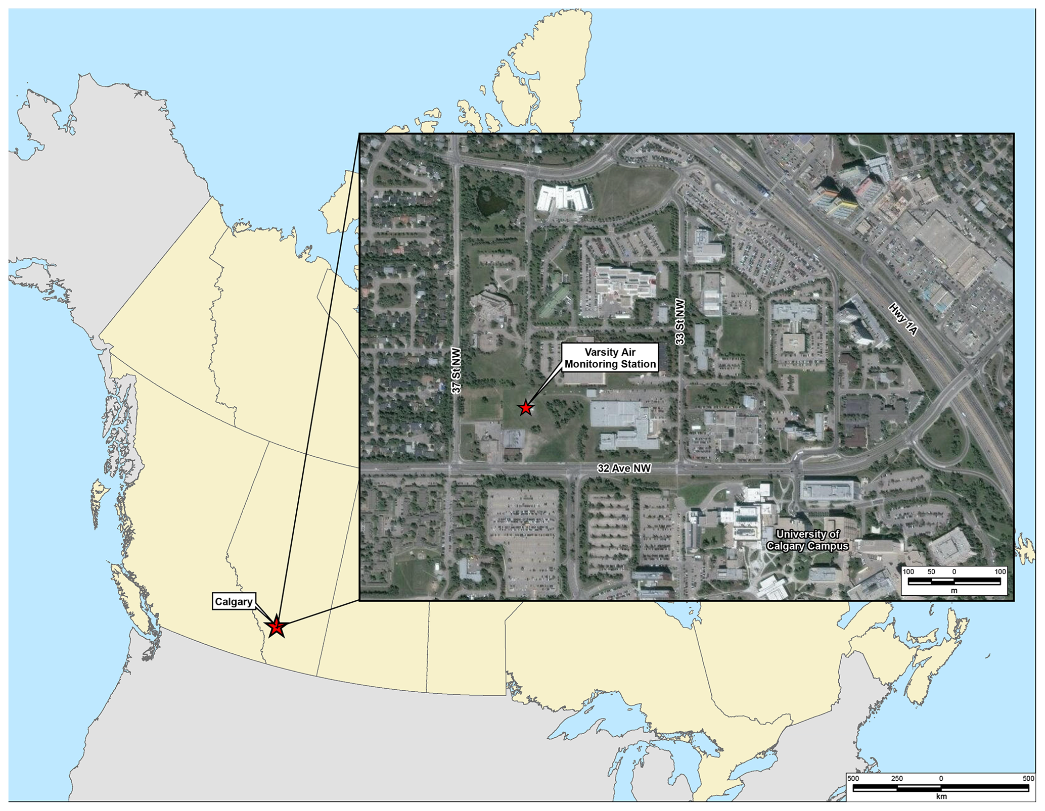
Figure 2Location of the Varsity air monitoring station. The map was created using ArcGIS®. The administrative boundaries in Canada and imagery data were provided by Natural Resources Canada (2020) and DigitalGlobe (2019).
The reference instrument used to evaluate the low-cost sensor is a Thermal Fisher Scientific SHARP model 5030. The SHARP instrument was installed at the Calgary Varsity station by CRAZ. The SHARP instrument continuously uses two compatible technologies, light scattering and beta attenuation, to measure PM2.5 every 6 min with an accuracy of ±5 %. The SHARP instrument is operated and maintained by CRAZ in accordance with the provincial government's guidelines outlined in Alberta's air monitoring directive. The instrument was calibrated monthly. Hourly PM2.5 data are published on the Alberta Air Data Warehouse website (http://www.airdata.alberta.ca/, last access: 3 June 2019). The Calgary Varsity station also continuously monitors CO, methane, oxides of nitrogen, non-methane hydrocarbons, outdoor air temperature, O3, RH, total hydrocarbon, wind direction, and wind speed. Detailed information on the analytical systems for the CRAZ Varsity station can be found on their website (https://craz.ca/monitoring/info-calgary-nw/, last access: 3 June 2019).
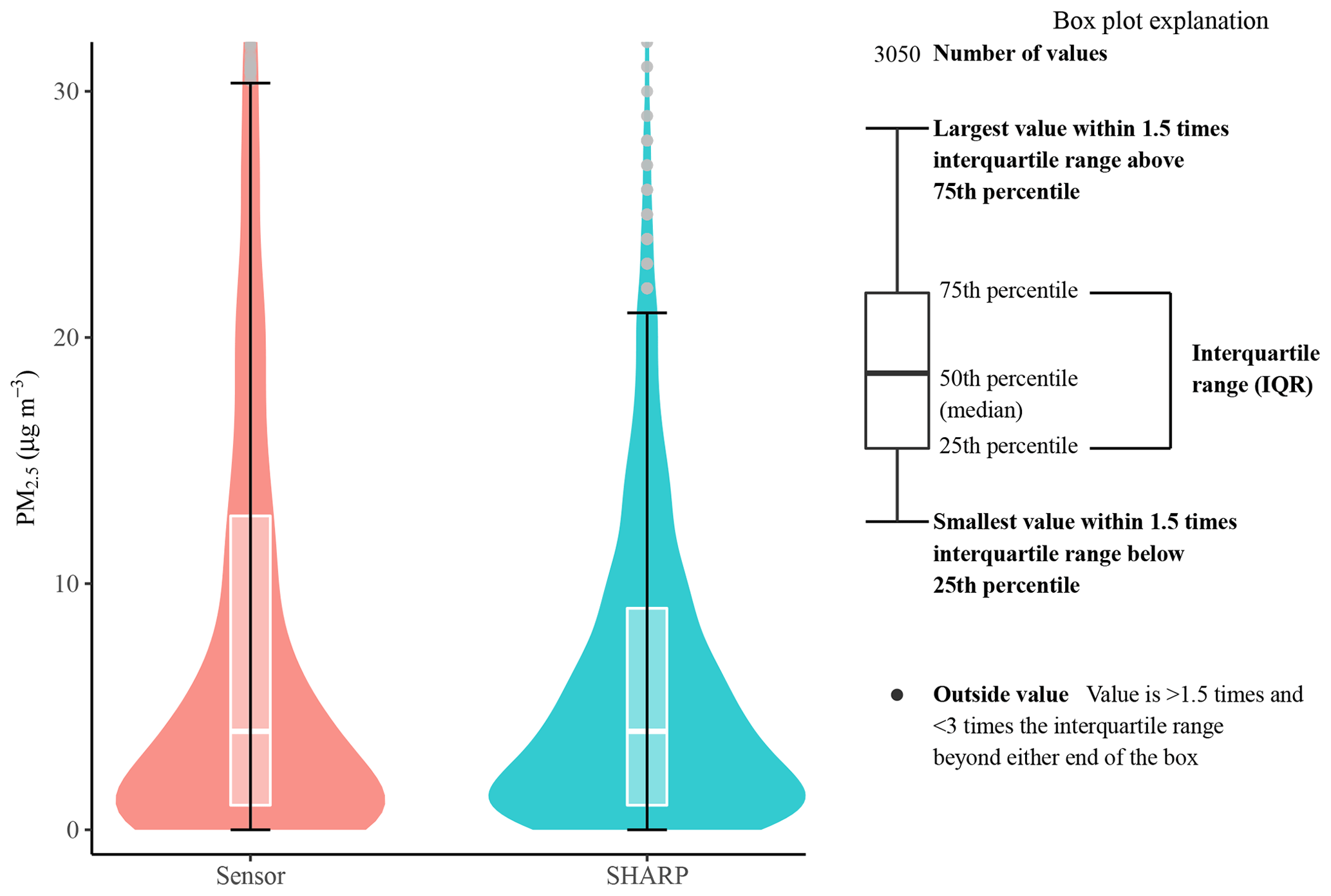
Figure 4Comparison of the hourly PM2.5 values between the low-cost PM sensor and SHARP. Based on 3050 hourly paired data points. The low-cost sensor has 250 hourly data points greater than 30 µg m−3. SHARP has 174 hourly data points greater than 20 µg m−3. Bars indicate the 25th and 75th percentile values, whiskers extend to values within 1.5 times the interquartile range (IQR), and dots represent values outside the IQR. The box plot explanation on the right is adjusted from DeCicco (2016).
The meteorological parameters in this study measured by the SHARP instrument are presented in Table 1.
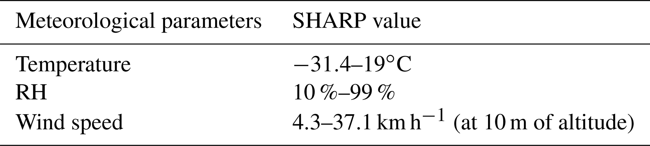

Figure 5PM2.5, relative humidity, and temperature data on the basis of a 24 h rolling average.
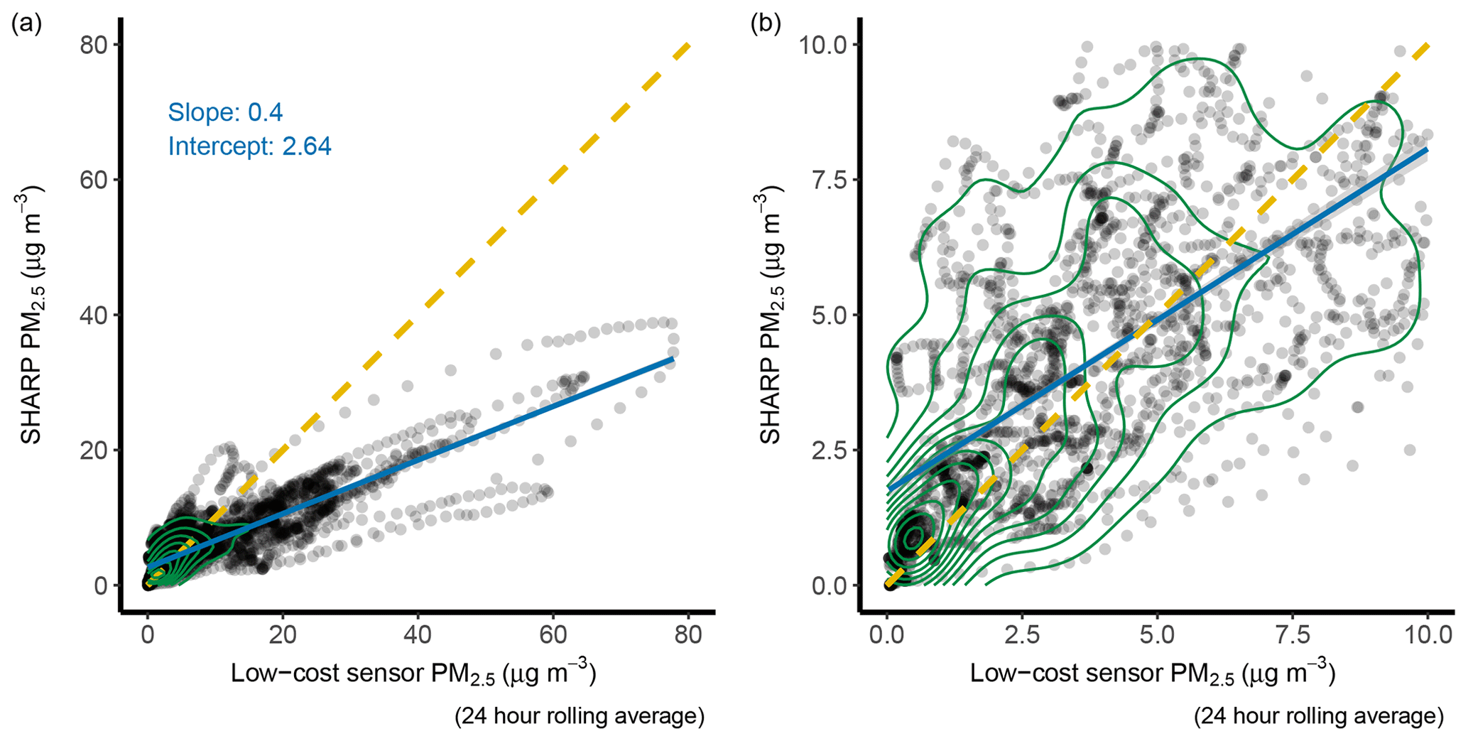
Figure 6SHARP versus low-cost sensor PM2.5 concentration (µg m−3). The yellow dashed line is a 1:1 line. The solid blue line is a regression line. Panel (a) is in full scale, and panel (b) is a zoom-in plot of panel (a). The green circle represents data density.
The following steps were taken to process the raw data from 00:00 on 7 December 2018 to 23:00 on 26 April 2019.
-
The 6 s interval data recorded by the low-cost sensor, including PM2.5, temperature, and RH, were averaged into hourly data to pair with SHARP data because only hourly SHARP data are publicly available.
-
The hourly sensor data and hourly SHARP data were combined into one structured data table. PM2.5, temperature, and RH by the low-cost sensor as well as PM2.5 by SHARP columns in the data table were selected. The data table then contains 3384 rows and four columns. Each row represents one hourly data point. The columns include the data measured by the low-cost sensor and the SHARP instrument.
-
Rows in the data table with missing values were removed – 299 missing values for PM2.5 from the low-cost sensor and 36 missing values for PM2.5 from the SHARP instrument. The reason for missing data from the SHARP instrument is the calibration. However, the reason for missing data from the low-cost sensor is unknown.
-
The data used for NN were transformed by z standardization with a mean of zero and a standard deviation of 1.
After the above steps, the processed data table with 3050 rows and four columns was used for evaluation and calibration. The data file is provided in the Supplement to this paper. Each row represents one example or sample for training or testing by the calibration methods.
2.2 Low-cost sensor evaluation
The Pearson correlation coefficient was used to compare the correlation for PM2.5 values between the low-cost sensor and the SHARP. SHARP was the reference method. The PM2.5 data by the low-cost sensor and SHARP were also compared using root mean square error (RMSE), mean square error (MSE), and mean absolute error (MAE).
The Fligner and Killeen test (F–K test) was used to evaluate the equality (homogeneity) of variances for PM2.5 values between the low-cost sensor and the SHARP instrument (Fligner and Killeen, 1976). The F–K test is a superior option in terms of robustness and power when data are non-normally distributed, the population means are unknown, or outliers cannot be removed (Conover et al., 1981; de Smith, 2018). The null hypothesis of the F–K test is that all populations' variances are equal; the alternative hypothesis is that the variances are statistically significantly different.
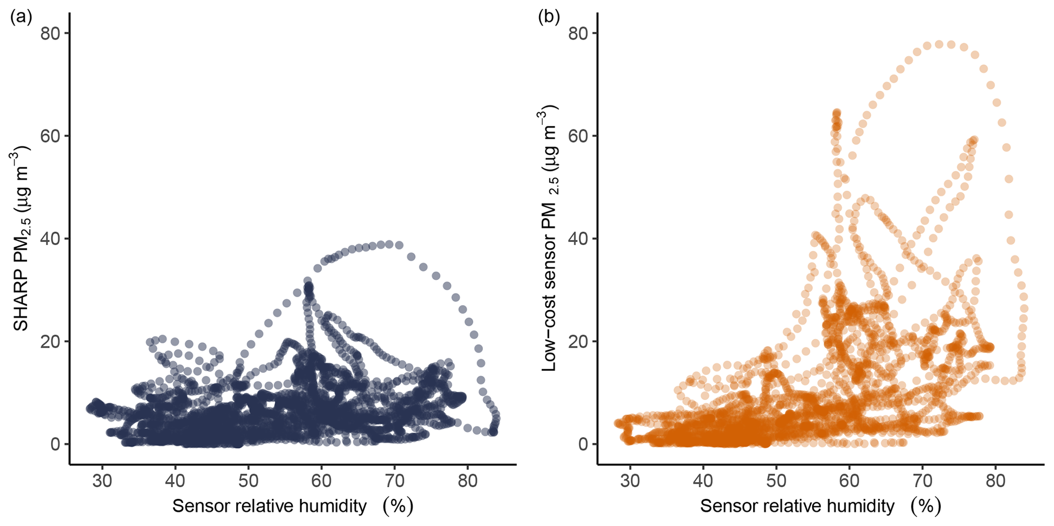
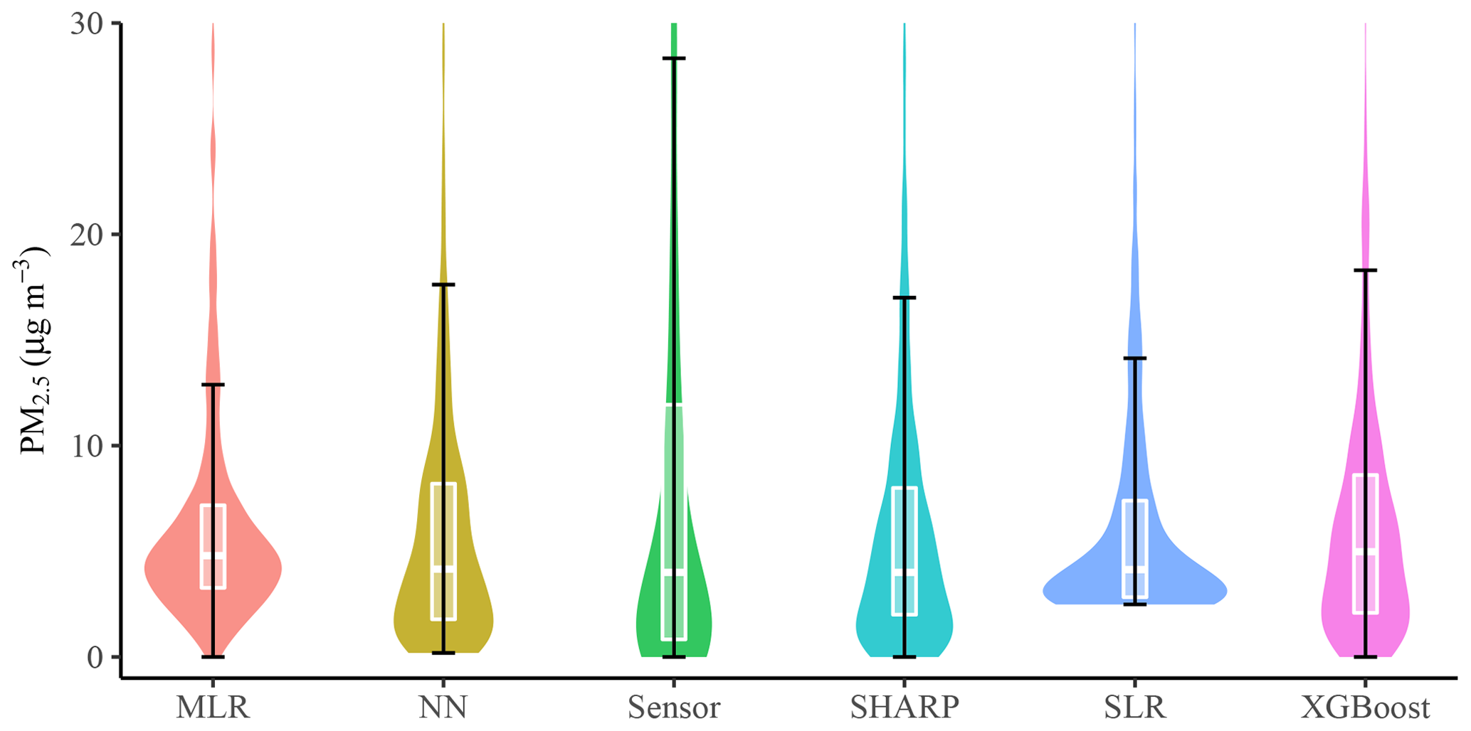
Figure 8Data density comparison in the test dataset. Based on 610 test examples. NN: neural network, MLR: multiple linear regression, SLR: simple linear regression. PM2.5 data greater than 30 µg m−3 are not shown in the figure. See the box plot explanation in Fig. 4.
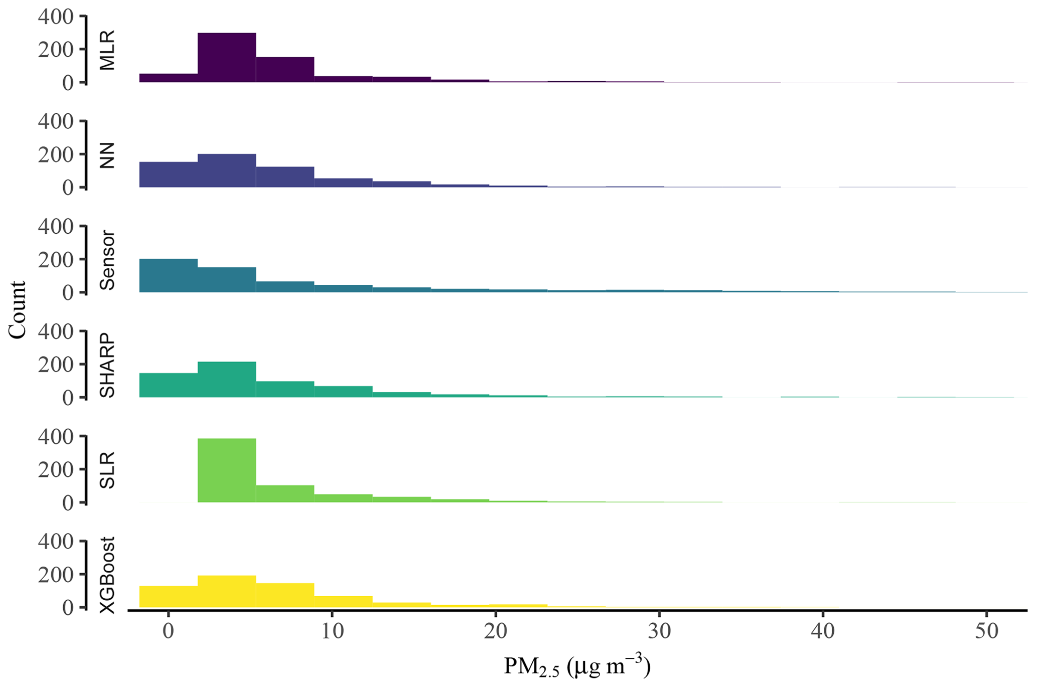
Figure 9Data distribution comparison. Based on 610 test examples. NN: neural network, MLR: multiple linear regression, SLR: simple linear regression.
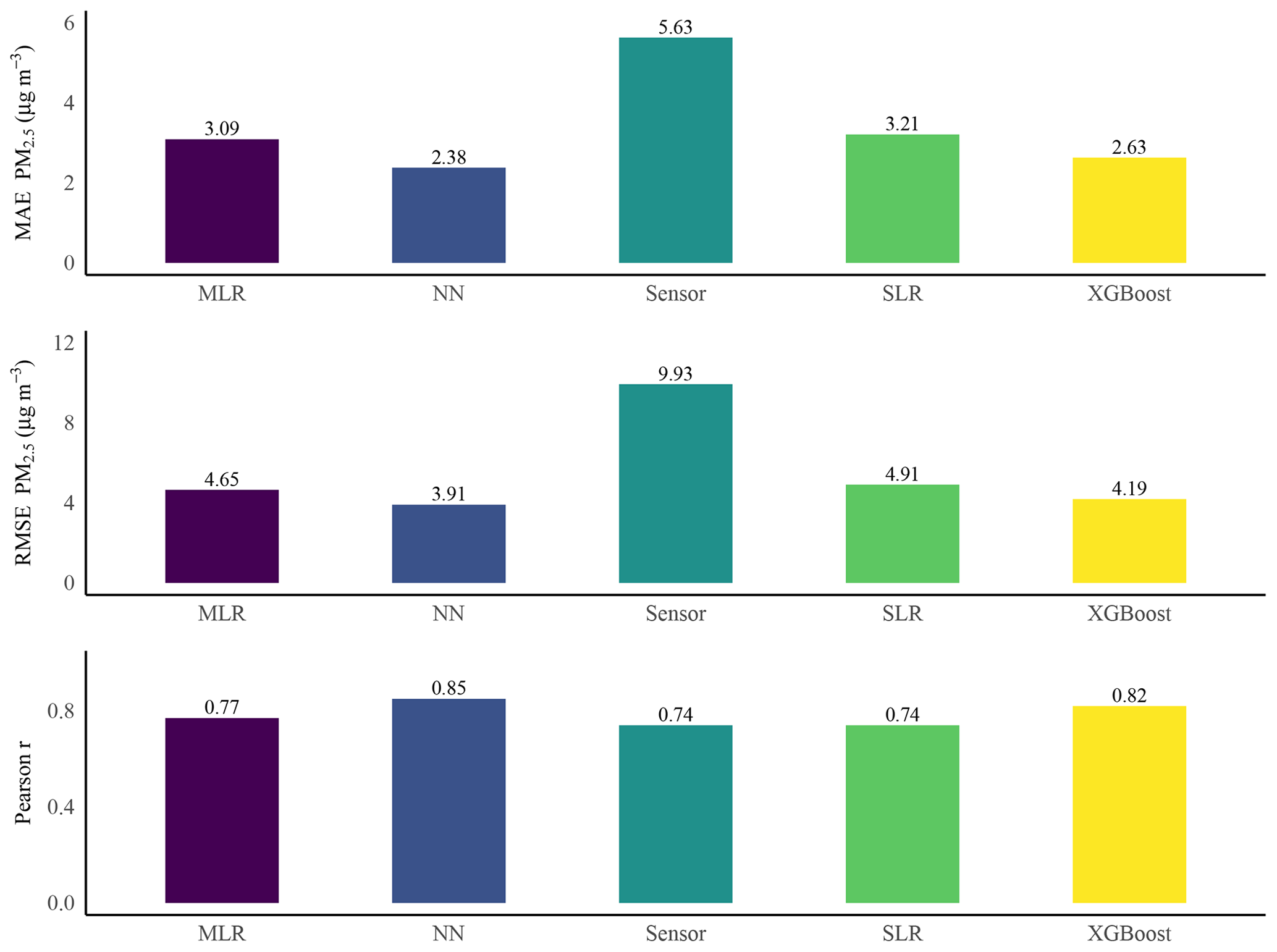
Figure 10Performances of different calibration methods. Based on 610 test examples. NN: neural network, MLR: multiple linear regression, SLR: simple linear regression.
2.3 Calibration
Four calibration methods were evaluated: SLR, MLR, XGBoost, and NN. Some predictions from the SLR, MLR, and XGBoost have negative values because they extrapolate observed values and regression is unbounded. When the predicted PM2.5 values generated by these calibration methods were negative, the negative values were replaced with the sensor data.
MLR, XGBoost, and feedforward NN use the PM2.5, temperature, and RH data measured by the low-cost sensor as inputs. The PM2.5 measured by the SHARP instrument is used as the target to supervise the machine-learning process. The processed dataset, with 3050 rows and four columns, was randomly shuffled and then divided into a training set, which was composed of the data used to build models and minimize the loss function, and a test set, which was composed of the data that the model had never been run with before testing (Si et al., 2019). The test dataset was only used once and gave an unbiased evaluation of the final model's performance. The evaluation was to test the ability of the machine-learning model to provide sensible predictions with new inputs (LeCun et al., 2015). The training dataset had 2440 examples (samples). The test dataset had 610 examples (samples).
2.3.1 Simple linear regression and multiple linear regression
The calibration by an SLR used Eq. (1).
β0 and β1 are the model coefficients and were calculated using the training dataset; is a model-predicted (calibrated) value. PM2.5 is the value measured by the low-cost sensor.
The MLR used PM2.5, RH, and temperature measured by the low-cost sensor as predictors because the low-cost sensor only measured these parameters. The model is expressed as Eq. (2).
The model coefficients, β0 to β3, were calculated using the training dataset with SHARP-provided readings as . The outputs of the models generated by the SLR and MLR were evaluated by comparing to the SHARP readings in the test dataset.
Table 2Calibration results by SLR and MLR using the test dataset.
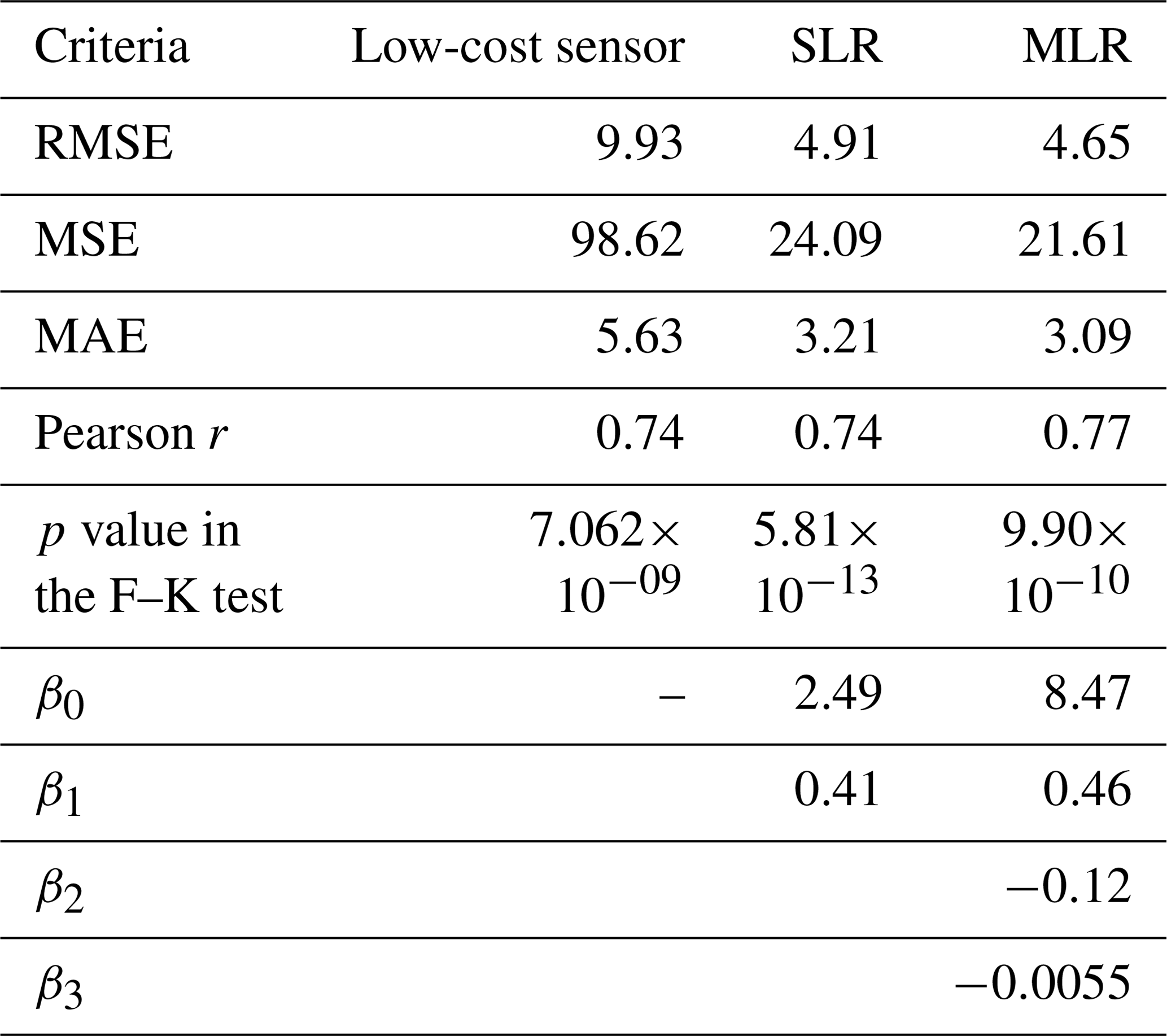
Note: the test dataset contains 660 examples.
2.3.2 XGBoost
XGBoost is a scalable decision-tree-based ensemble algorithm, and it uses a gradient boosting framework (Chen and Guestrin, 2016). The XGBoost was implemented using the XGBoost (version 0.90) and scikit-learn (version 0.21.2) packages in Python (version 3.7.3). A random search method (Bergstra and Bengio, 2012) was used to tune the hyperparameters in the XGBoost algorithm, and the hyperparameters tuned include the following:
-
the number of trees to fit (n_estimator);
-
the maximum depth of a tree (max_depth);
-
the step size shrinkage used in an update (learning_rate);
-
the subsample ratio of columns when constructing each tree (colsample_bytree);
-
the minimum loss reduction required to make a further partition on a leaf node of the tree (gamma);
-
L2 regularization on weights (reg_lambda); and
-
the minimum sum of instance weight needed in a child (min_child_ weight).
A detailed explanation of each hyperparameter is provided in the XGBoost documentation (XGBoost developers, 2019). The 10-fold cross-validation was used to select the best model with minimum MSE from the random search. The best model was then evaluated against the SHARP PM2.5 data using the test dataset.
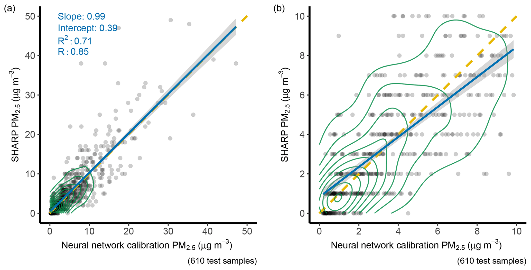
Figure 11Comparison between the NN predictions and SHARP. Based on 610 test examples. Panel (a) is in full scale. Panel (b) is a zoom-in plot of panel (a). The solid blue line is a regression line. The yellow dashed line is a 1:1 line. The green circle represents data density. The grey area along the regression line represents 1 standard deviation.
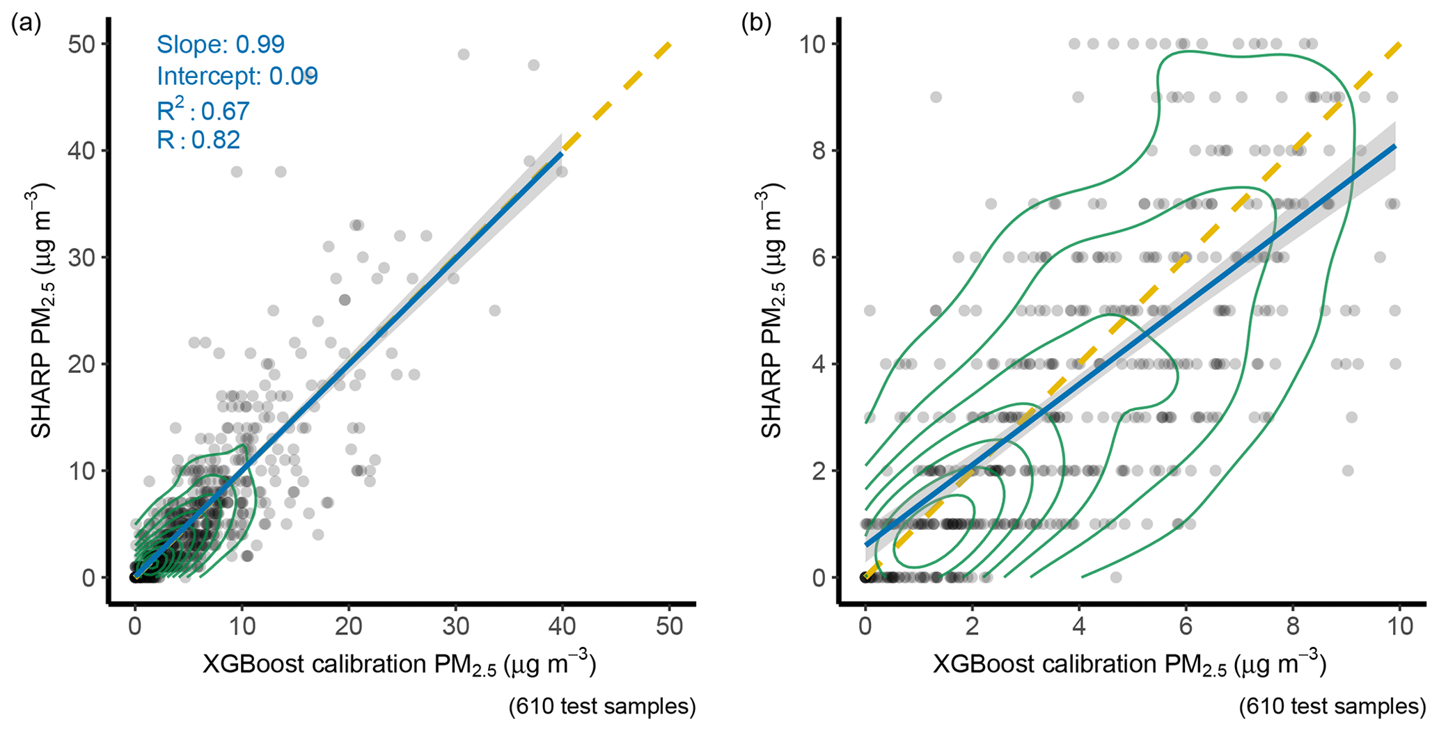
Figure 12Comparison between the XGBoost predictions and SHARP. Based on 610 test examples. NN: neural network. Panel (a) is in full scale. Panel (b) is a zoom-in plot of panel (a). The solid blue line is a regression line. The yellow dashed line is a 1:1 line. The green circle represents data density. The grey area along the regression line represents 1 standard deviation.
2.3.3 Neural network
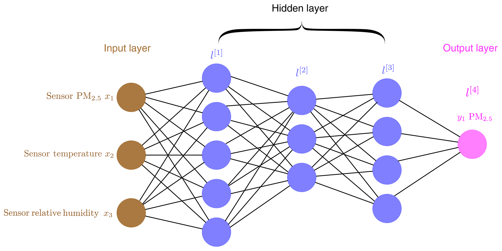
A fully connected feedforward NN architecture was used in the study. In a fully connected NN, each unit (node) in a layer is connected to each unit in the following layer. Data from the input layer are passed through the network until the unit(s) in the output layer is (are) reached. An example of a fully connected feedforward NN is presented in Fig. 3. A back-propagation algorithm is used to minimize the difference between the SHARP-measured values and the predicted values (Rumelhart et al., 1986).
The NN was implemented using the Keras (version 2.2.4) and TensorFlow (version 1.14.0) libraries in Python (version 3.7.3). Keras and TensorFlow were the most referenced deep-learning frameworks in scientific research in 2017 (RStudio, 2018). Keras is the front end of TensorFlow.
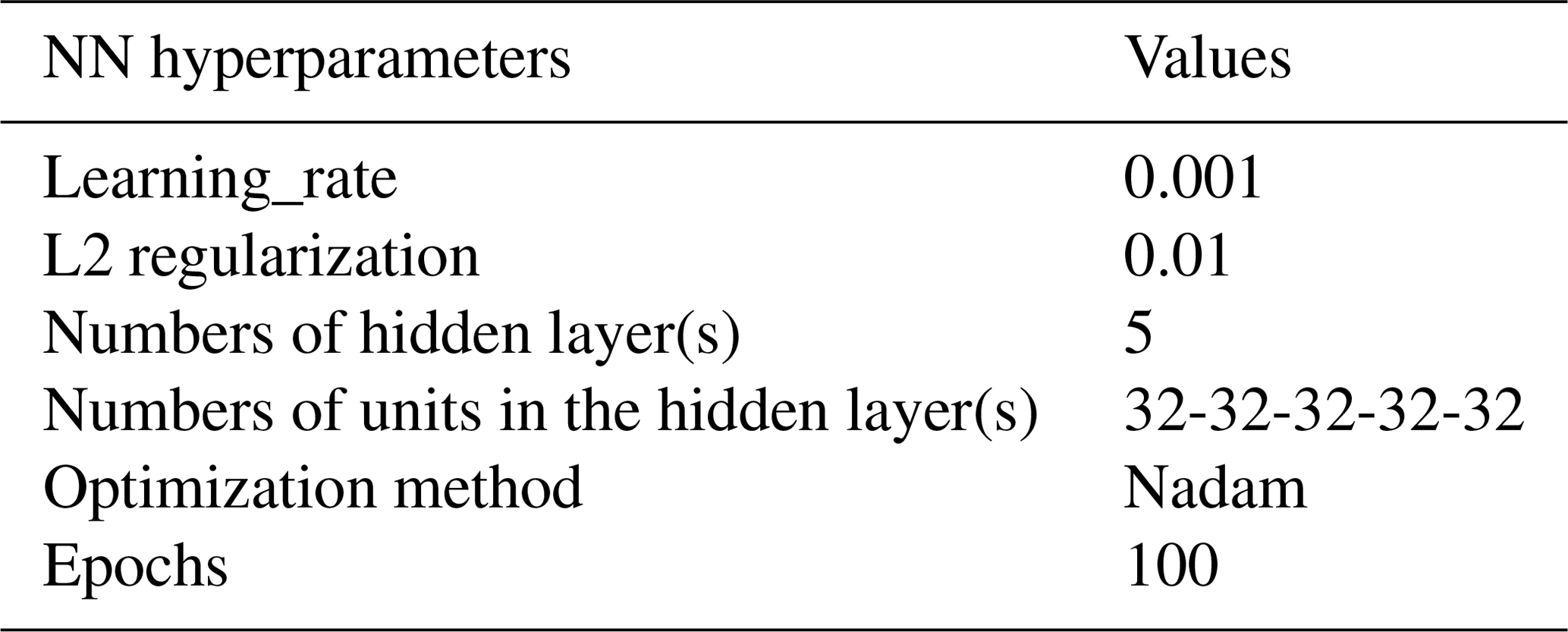
The learning rate, L2 regularization rate, number of hidden layers, number of units in the hidden layers, and optimization methods were tuned using the random search method provided in the scikit-learn machine-learning library. A 10-fold cross-validation was used to evaluate the models. The model with the minimum MSE was considered to be the best-fit model and then used for model testing.
3.1 Sensor evaluation
3.1.1 Hourly data
The RMSE, MSE, and MAE between the low-cost sensor and SHARP for the hourly PM2.5 data were 10.58, 111.83, and 5.74. The Pearson correlation coefficient r value was 0.78. The PM2.5 concentrations by the sensor ranged from 0 to 178 µg m−3 with a standard deviation of 14.90 µg m−3 and a mean of 9.855 µg m−3. The PM2.5 concentrations by SHARP ranged from 0 to 80 µg m−3 with a standard deviation of 7.80 and a mean of 6.55 µg m−3. Both SHARP and the low-cost sensor dataset had a median of 4.00 µg m−3 based on hourly data (Fig. 4). The violin plot in Fig. 4 describes the distribution of the PM2.5 values measured by the low-cost sensor and SHARP using a density curve. The width of each curve represents the frequency of PM2.5 values at each concentration level. The p value from the F–K test was less than , indicating that the variance of the PM2.5 values measured by the low-cost sensor was statistically significantly different from the variance of the PM2.5 values measured by the SHARP instrument.
3.1.2 24 h rolling average data
Over 24 h, the median value for SHARP was 5.38 µg m−3, and for the low-cost sensor it was 5.01 µg m−3. Over 5 months (December 2018 to April 2019), the low-cost sensor tended to generate higher PM2.5 values compared to the SHARP monitoring data (Fig. 5)
When PM2.5 concentrations were greater than 10 µg m−3, the low-cost sensor consistently produced values that were higher than the reference method (Fig. 6). When the concentrations were less than 10 µg m−3, the performance of the low-cost sensor was close to the reference method, producing slightly smaller values (Fig. 6)
3.2 Calibration by simple linear regression and multiple linear regression
The RMSE was 4.91 calibrated by SLR and 4.65 by MLR (Table 2). The r value was 0.74 by SLR and 0.77 by MLR. The p values in the F–K test by the SLR and MLR were less than 0.05, which suggested that the variances of the PM2.5 values were statistically significantly different.
3.3 Calibration by XGBoost
The hyperparameters selected by the random search for the best model using XGBoost are presented in Table 3.
In the training dataset, the RMSE was 3.03, and the MAE was 1.93 by the best XGBoost model. The RMSE in the test dataset was reduced by 57.8 % using the XGBoost from 9.93 by the sensor to 4.19 (Table 4). The p value in the F–K test using the test dataset was 0.7256, which showed no evidence that the PM2.5 values varied with statistical significance between the XGBoost-predicted values and SHARP-measured values.
3.4 Calibration by neural network
The hyperparameters for the best NN model are presented in Table 5.
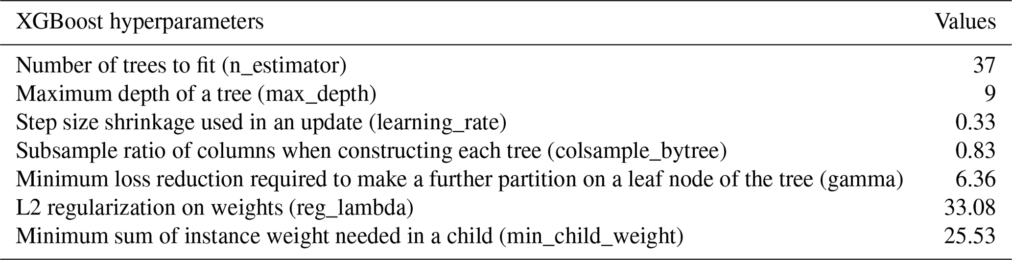
Table 4Table 4: calibration results by XGBoost using the test dataset.
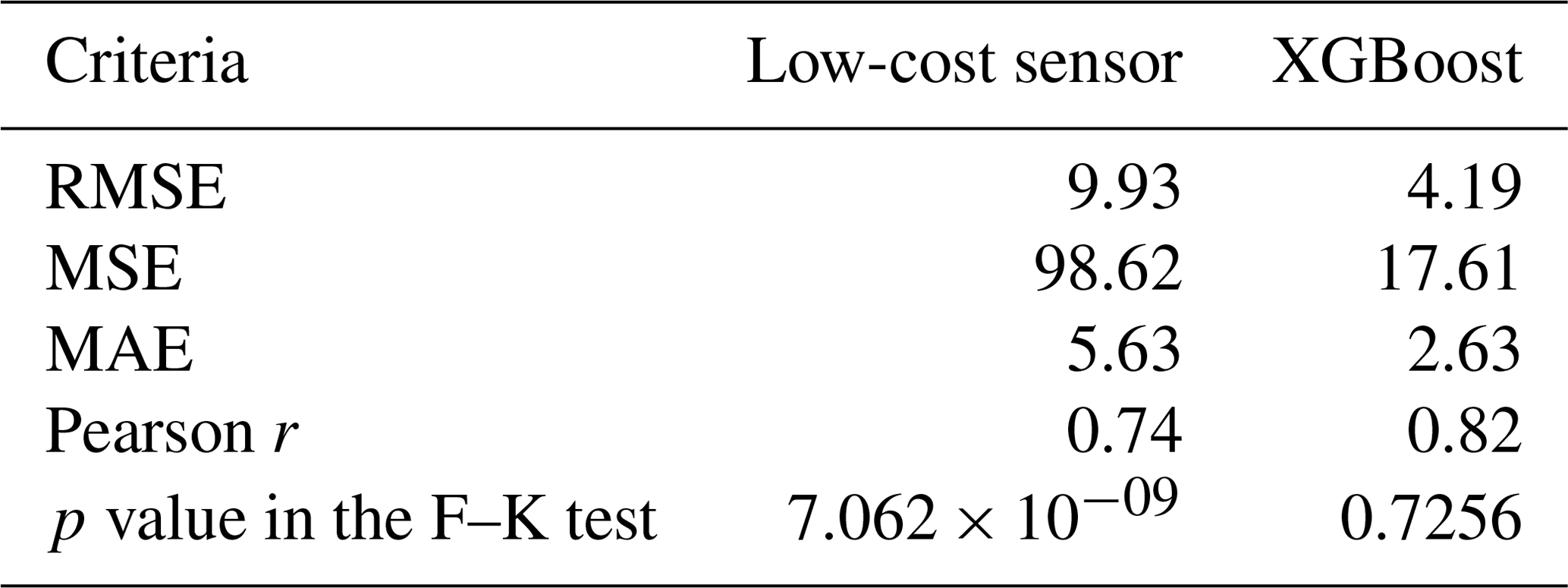
Note: the test dataset contains 610 examples.
In the training dataset, the RMSE was 3.22, and the MAE was 2.17 by the best NN-based model. The RMSE was reduced by 60 % using the NN from 9.93 to 3.91 in the test dataset (Table 6). The p value in the F–K test was 0.43, which suggested that the variances in the PM2.5 values were not statistically significantly different between the NN-predicted values and SHARP-measured values.
Table 6Calibration results by the neural network using the test dataset.
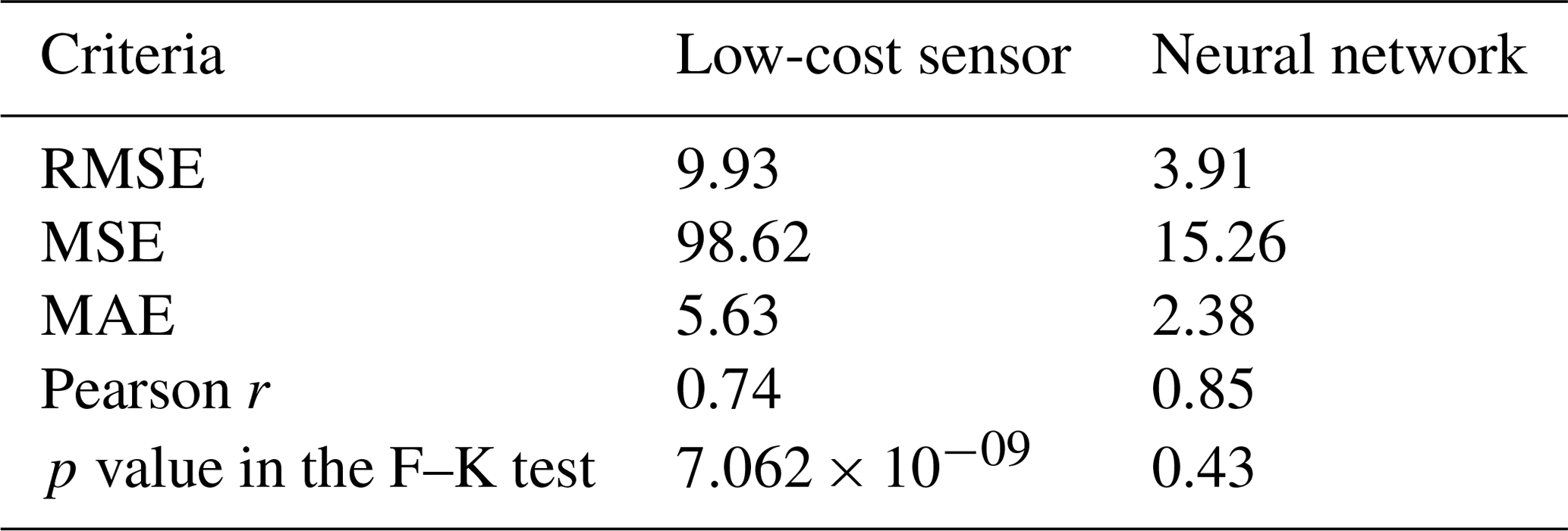
Note: the test dataset includes 610 examples.
Table 7Descriptive statistics by season.
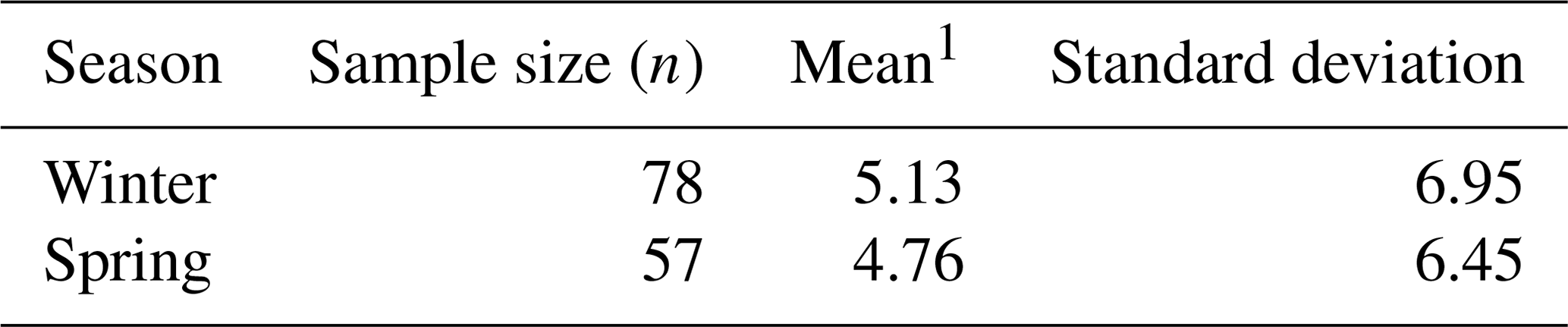
Note: (1) the mean is calculated by .
3.5 Discussion
3.5.1 Relative humidity impact
RH has significant effects on the low-cost sensor's responses. The RH trend matched the low-cost sensor's PM2.5 trend closely. The spikes in the low-cost sensor's PM2.5 trend corresponded with increases in RH values, and the low-cost sensor tended to produce inaccurately high PM2.5 values when RH suddenly increased (Fig. 5). However, the relationship between PM2.5 and RH was not linear (Fig. 7)
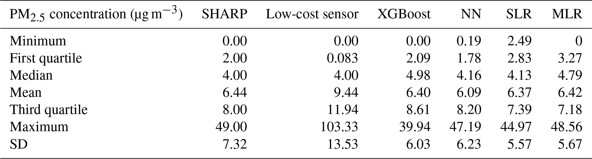
Table 8Descriptive statistics of PM2.5 concentrations using the test dataset.
3.5.2 Seasonal impact
We assessed the seasonal impact on the low-cost sensor by comparing the means of absolute differences between the daily average of sensor values and the daily average of SHARP values in winter (December 2018 to February 2019) and spring (March 2019 to April 2019). A descriptive statistic is presented in Table 7.
We used a two-sample t test to assess whether the means of absolute differences for winter and spring were equal. The p value of the t test was 0.754. Because , we retained the null hypothesis. There was not sufficient evidence at the α=0.05 level to conclude that the means of absolute differences between the low-cost sensor and SHARP values were significantly different for winter and spring.
3.5.3 Calibration assessment
Descriptive statistics of the PM2.5 concentrations in the test dataset for SHARP, the low-cost sensor, XGBoost, NN, SLR, and MLR are presented in Table 8. The arithmetic mean of the PM2.5 concentrations measured by the low-cost sensor was 9.44 µg m−3. In contrast, the means of the PM2.5 concentrations were 6.44 µg m−3 by SHARP, 6.40 µg m−3 by XGBoost, and 6.09 µg m−3 by NN.
NN and XGBoost produced data distributions that were similar to SHARP (Fig. 8). SLR had the worst performance. Fig. 9 shows that SLR could not predict low concentrations. The predictions made by NN and XGBoost ranged from 0.19 to 47.19 µg m−3 and from 0.00 to 39.94 µg m−3.
In the test dataset, the NN produced the lowest MAE of 2.38 (Fig. 10). The MAEs were 2.63 by XGBoost, 3.09 by MLR, and 3.21 by SLR when compared with the PM2.5 data measured by the SHARP instrument. The NN also had the lowest RMSE score in the test dataset. The RMSEs were 3.91 for the NN, 4.19 for XGBoost, and 9.93 for the low-cost sensor (Fig. 10). The Pearson r value by the NN was 0.85 compared to 0.74 by the low-cost sensor.
The XGBoost and NN machine-learning algorithms have a better performance compared to traditional SLR and MLR calibration methods. NN calibration reduced the RMSE by 60 %. Both NN and XGBoost demonstrated the ability to correct the bias for high concentrations made by the low-cost sensor (Figs. 11 and 12). Most of the values that were greater than 10 µg m−3 in the NN model fall closer to the yellow 1:1 line (Fig. 11). NN had slightly better performance for low concentrations compared to XGBoost.
In this study, we evaluated one low-cost sensor against a reference instrument – SHARP – using 3050 hourly data points from 00:00 on 7 December 2018 to 23:00 on 26 April 2019. The p value from the F–K test suggested that the variances in the PM2.5 values were statistically significantly different between the low-cost sensor and the SHARP instrument. Based on the 24 h rolling average, the low-cost sensor in this study tended to report higher PM2.5 values compared to the SHARP instrument. The low-cost sensor had a strong bias when PM2.5 concentrations were greater than 10 µg m−3. The study also showed that the sensor's bias responses are likely caused by the sudden changes in RH.
Four calibration methods were tested and compared: SLR, MLR, NN, and XGBoost. The p values from the F–K tests for the XGBoost and NN were greater than 0.05, which indicated that, after calibration by the XGBoost and the NN, the variances of the PM2.5 values were not statistically significantly different from the variance of the PM2.5 values measured by the SHARP instrument. In contrast, the p values from the F–K tests for the SLR and MLR were still less than 0.05. The NN generated the lowest RMSE score in the test dataset with 610 samples. The RMSE by NN was 3.91, the lowest of the four methods. RMSEs were 4.91 by SLR, 4.65 by MLR, and 4.19 by XGBoost.
However, a wide installation of low-cost sensors may still face challenges, including the following.
-
Durability of the low-cost sensor. The low-cost sensor used in the study was deployed in the ambient environment. We installed four sensors between 7 December 2018 and 20 June 2019. Only one sensor lasted approximately 5 months; the data from this sensor were used in this study. The other three sensors only lasted 2 weeks to 1 month and collected limited data. These three sensors did not collect enough data for machine learning and were therefore not used in this study.
-
Missing data. In this study, the low-cost sensor dataset has 299 missing values for PM2.5 concentrations. The reason for the missing data is unknown.
-
Transferability of machine-learning models. The models developed by the two more powerful machine-learning algorithms that were used to calibrate the low-cost sensor data tend to be sensor-specific because of the nature of machine learning. Further research is needed to test the transferability of the models for broader use.
The hourly sensor data and hourly SHARP data are provided online at https://doi.org/10.5281/zenodo.3473833 (Si, 2019).
MS conducted the evaluation and calibrations. YX installed the sensor and monitored and collected the sensor data. MS and YX wrote the paper together and made an equal contribution. SD edited the machine-learning methods. KD secured the funding and supervised the project. All authors discussed the results and commented on the paper.
The authors declare that they have no conflict of interest.
Reference to any companies or specific commercial products does not constitute endorsement or recommendation by the authors.
The authors wish to thank SensorUp for providing the low-cost sensors and the Calgary Region Airshed Zone air quality program manager Mandeep Dhaliwal for helping with the installation of the PM sensors and a 4G LTE router, as well as the collection of the SHARP data. The authors would also like to thank Jessica Coles for editing an earlier version of this paper.
This research has been supported by the Natural Sciences and Engineering Research Council of Canada (grant nos. EGP 521823–17 and CRDPJ 535813-18).
This paper was edited by Keding Lu and reviewed by four anonymous referees.
Bergstra, J. and Bengio, Y.: Random Search for Hyper-Parameter Optimization, J. Mach. Learn. Res., 13, 281–305, 2012.
CDNova Instrument Ltd.: SHARP Cost Estimate, Calgary, Canada, 2017.
Charlson, R. J., Schwartz, S. E., Hales, J. M., Cess, R. D., Coakley, J. A., Hansen, J. E., and Hofmann, D. J.: Climate Forcing by Anthropogenic Aerosols, Science, 255, 423–430, https://doi.org/10.1126/science.255.5043.423, 1992.
Chen, T. and Guestrin, C.: XGBoost: A Scalable Tree Boosting System, in: Proceedings of the 22nd ACM SIGKDD International Conference on Knowledge Discovery and Data Mining – KDD '16, 785–794, ACM Press, San Francisco, California, USA, 2016.
Chong, C.-Y. and Kumar, S. P.: Sensor networks: Evolution, opportunities, and challenges, Proc. IEEE, 91, 1247–1256, https://doi.org/10.1109/JPROC.2003.814918, 2003.
Chow, J. C. and Watson, J. G.: Guideline on Speciated Particulate Monitoring, available at: https://www3.epa.gov/ttn/amtic/files/ambient/pm25/spec/drispec.pdf (last access: 17 September 2019), 1998.
Conover, W. J., Johnson, M. E., and Johnson, M. M.: A Comparative Study of Tests for Homogeneity of Variances, with Applications to the Outer Continental Shelf Bidding Data, Technometrics, 23, 351–361, https://doi.org/10.1080/00401706.1981.10487680, 1981.
Cordero, J. M., Borge, R., and Narros, A.: Using statistical methods to carry out in field calibrations of low cost air quality sensors, Sensor Actuat. B-Chem., 267, 245–254, https://doi.org/10.1016/j.snb.2018.04.021, 2018.
DeCicco, L.: Exploring ggplot2 boxplots – Defining limits and adjusting style, available at: https://owi.usgs.gov/blog/boxplots/ (last access: 18 September 2019), 2016.
de Smith, M.: Statistical Analysis Handbook, 2018 Edition, The Winchelsea Press, Drumlin Security Ltd, Edinburgh, available at: http://www.statsref.com/HTML/index.html?fligner-killeen_test.html (last access: 7 September 2019), 2018.
De Vito, S., Massera, E., Piga, M., Martinotto, L., and Di Francia, G.: On field calibration of an electronic nose for benzene estimation in an urban pollution monitoring scenario, Sensor Actuat. B-Chem., 129, 750–757, https://doi.org/10.1016/j.snb.2007.09.060, 2008.
De Vito, S., Piga, M., Martinotto, L., and Di Francia, G.: CO, NO2 and NOx urban pollution monitoring with on-field calibrated electronic nose by automatic bayesian regularization, Sensor Actuat. B-Chem., 143, 182–191, https://doi.org/10.1016/j.snb.2009.08.041, 2009.
De Vito, S., Esposito, E., Salvato, M., Popoola, O., Formisano, F., Jones, R., and Di Francia, G.: Calibrating chemical multisensory devices for real world applications: An in-depth comparison of quantitative machine learning approaches, Sensor Actuat. B-Chem., 255, 1191–1210, https://doi.org/10.1016/j.snb.2017.07.155, 2018.
DigitalGlobe: ESRI World Imagery Basemap Service, Environmental Systems Research Institute (ESRI), Redlands, California USA, 2019.
Esposito, E., De Vito, S., Salvato, M., Bright, V., Jones, R. L., and Popoola, O.: Dynamic neural network architectures for on field stochastic calibration of indicative low cost air quality sensing systems, Sensor Actuat. B-Chem., 231, 701–713, https://doi.org/10.1016/j.snb.2016.03.038, 2016.
Fligner, M. A. and Killeen, T. J.: Distribution-Free Two-Sample Tests for Scale, J. Am. Stat. Assoc., 71, 210–213, https://doi.org/10.1080/01621459.1976.10481517, 1976.
Government of Canada: National Air Pollution Surveillance (NAPS) Network – Open Government Portal, Natl. Air Pollut. Surveill. NAPS Netw., available at: https://open.canada.ca/data/en/dataset/1b36a356-defd-4813-acea-47bc3abd859b, last access: 17 September 2019.
Holstius, D. M., Pillarisetti, A., Smith, K. R., and Seto, E.: Field calibrations of a low-cost aerosol sensor at a regulatory monitoring site in California, Atmos. Meas. Tech., 7, 1121–1131, https://doi.org/10.5194/amt-7-1121-2014, 2014.
Jayaratne, R., Liu, X., Thai, P., Dunbabin, M., and Morawska, L.: The influence of humidity on the performance of a low-cost air particle mass sensor and the effect of atmospheric fog, Atmos. Meas. Tech., 11, 4883–4890, https://doi.org/10.5194/amt-11-4883-2018, 2018.
Krizhevsky, A., Sutskever, I., and Hinton, G. E.: ImageNet classification with deep convolutional neural networks, Commun ACM, 60, 84–90, 2017.
Kumar, P., Morawska, L., Martani, C., Biskos, G., Neophytou, M., Di Sabatino, S., Bell, M., Norford, L., and Britter, R.: The rise of low-cost sensing for managing air pollution in cities, Environ. Int., 75, 199–205, https://doi.org/10.1016/j.envint.2014.11.019, 2015.
LeCun, Y., Bengio, Y., and Hinton, G.: Deep learning, Nature, 521, 436–444, https://doi.org/10.1038/nature14539, 2015.
Lewis, A. C., Lee, J. D., Edwards, P. M., Shaw, M. D., Evans, M. J., Moller, S. J., Smith, K. R., Buckley, J. W., Ellis, M., Gillot, S. R., and White, A.: Evaluating the performance of low cost chemical sensors for air pollution research, Faraday Discuss., 189, 85–103, https://doi.org/10.1039/C5FD00201J, 2016.
Lin, Y., Dong, W., and Chen, Y.: Calibrating Low-Cost Sensors by a Two-Phase Learning Approach for Urban Air Quality Measurement, Proc. ACM Interact. Mob. Wearable Ubiquitous Technol., 2, 1–18, https://doi.org/10.1145/3191750, 2018.
Loh, B. G. and Choi, G.-H.: Calibration of Portable Particulate Matter – Monitoring Device using Web Query and Machine Learning, Saf. Health Work, 10, S2093791119302811, https://doi.org/10.1016/j.shaw.2019.08.002, 2019.
Maag, B., Zhou, Z., and Thiele, L.: A Survey on Sensor Calibration in Air Pollution Monitoring Deployments, IEEE Internet Things J., 5, 4857–4870, https://doi.org/10.1109/JIOT.2018.2853660, 2018.
Natural Resources Canada: Administrative Boundaries in Canada – CanVec Series – Administrative Features, available at: https://open.canada.ca/data/en/dataset/306e5004-534b-4110-9feb-58e3a5c3fd97, last access: 5 March 2020.
Papapostolou, V., Zhang, H., Feenstra, B. J., and Polidori, A.: Development of an environmental chamber for evaluating the performance of low-cost air quality sensors under controlled conditions, Atmos. Environ., 171, 82–90, https://doi.org/10.1016/j.atmosenv.2017.10.003, 2017.
Patashnick, H. and Rupprecht, E. G.: Continuous PM10 Measurements Using the Tapered Element Oscillating Microbalance, J. Air Waste Manag. Assoc., 41, 1079–1083, https://doi.org/10.1080/10473289.1991.10466903, 1991.
RStudio: Why Use Keras?, available at: https://keras.rstudio.com/articles/why_use_keras.html, last access: 11 November 2018.
Rumelhart, D. E., Hinton, G. E., and Williams, R. J.: Learning representations by back-propagating errors, Nature, 323, 533–536, https://doi.org/10.1038/323533a0, 1986.
Seinfeld, J. H. and Pandis, S. N.: Atmospheric chemistry and physics: from air pollution to climate change, Wiley, New York, 1998.
Si, M.: Evaluation and Calibration of a Low-cost Particle Sensor in Ambient Conditions Using Machine Learning Methods (Version v0), Data set, Zenodo, https://doi.org/10.5281/zenodo.3473833, 2019.
Si, M., Tarnoczi, T. J., Wiens, B. M., and Du, K.: Development of Predictive Emissions Monitoring System Using Open Source Machine Learning Library – Keras: A Case Study on a Cogeneration Unit, IEEE Access, 7, 113463–113475, https://doi.org/10.1109/ACCESS.2019.2930555, 2019.
Snyder, E. G., Watkins, T. H., Solomon, P. A., Thoma, E. D., Williams, R. W., Hagler, G. S. W., Shelow, D., Hindin, D. A., Kilaru, V. J., and Preuss, P. W.: The Changing Paradigm of Air Pollution Monitoring, Environ. Sci. Technol., 47, 11369–11377, https://doi.org/10.1021/es4022602, 2013.
Spinelle, L., Gerboles, M., Villani, M. G., Aleixandre, M., and Bonavitacola, F.: Field calibration of a cluster of low-cost available sensors for air quality monitoring. Part A: Ozone and nitrogen dioxide, Sensor Actuat. B-Chem., 215, 249–257, https://doi.org/10.1016/j.snb.2015.03.031, 2015.
Spinelle, L., Gerboles, M., Villani, M. G., Aleixandre, M., and Bonavitacola, F.: Field calibration of a cluster of low-cost commercially available sensors for air quality monitoring. Part B: NO, CO and CO2, Sensor Actuat. B-Chem., 238, 706–715, https://doi.org/10.1016/j.snb.2016.07.036, 2017.
Timbers, F.: Random Search for Hyper-Parameter Optimization, Finbarr Timbers, available at: https://finbarr.ca/random-search-hyper-parameter-optimization/ (last access: 4 October 2019), 2017.
US EPA: List of designated reference and equivalent methods, available at: https://www3.epa.gov/ttnamti1/files/ambient/criteria/AMTIC List Dec 2016-2.pdf (last access: 7 October 2019), 2016.
Wang, Y., Li, J., Jing, H., Zhang, Q., Jiang, J., and Biswas, P.: Laboratory Evaluation and Calibration of Three Low-Cost Particle Sensors for Particulate Matter Measurement, Aerosol Sci. Technol., 49, 1063–1077, https://doi.org/10.1080/02786826.2015.1100710, 2015.
White, R., Paprotny, I., Doering, F., Cascio, W., Solomon, P., and Gundel, L.: Sensors and “apps” for community-based: Atmospheric monitoring, EM Air Waste Manag. Assoc. Mag. Environ. Manag., 36–40, 2012.
Williams, R., Kaufman, A., Hanley, T., Rice, J., and Garvey, S.: Evaluation of Field-deployed Low Cost PM Sensors, U.S. Environmental Protection Agency, available at: https://cfpub.epa.gov/si/si_public_record_report.cfm?Lab{\textdollar}={\textdollar}NERL&DirEntryId=297517 (last access: 17 September 2019), 2014.
XGBoost developers: XGBoost Parameters – xgboost 1.0.0-SNAPSHOT documentation, available at: https://xgboost.readthedocs.io/en/latest/parameter.html (last access: 24 January 2020), 2019.
Xiong, Y., Zhou, J., Schauer, J. J., Yu, W., and Hu, Y.: Seasonal and spatial differences in source contributions to PM2.5 in Wuhan, China, Sci. Total Environ., 577, 155–165, https://doi.org/10.1016/j.scitotenv.2016.10.150, 2017.
Zheng, A.: Evaluating Machine Learning Models, First Edition., O'Reilly Media, Inc., 1005 Gravenstein Highway North, Sebastopol, CA, 2015.
Zheng, T., Bergin, M. H., Johnson, K. K., Tripathi, S. N., Shirodkar, S., Landis, M. S., Sutaria, R., and Carlson, D. E.: Field evaluation of low-cost particulate matter sensors in high- and low-concentration environments, Atmos. Meas. Tech., 11, 4823–4846, https://doi.org/10.5194/amt-11-4823-2018, 2018.
Zikova, N., Hopke, P. K., and Ferro, A. R.: Evaluation of new low-cost particle monitors for PM2.5 concentrations measurements, J. Aerosol Sci., 105, 24–34, https://doi.org/10.1016/j.jaerosci.2016.11.010, 2017.
Zimmerman, N., Presto, A. A., Kumar, S. P. N., Gu, J., Hauryliuk, A., Robinson, E. S., Robinson, A. L., and Subramanian, R.: A machine learning calibration model using random forests to improve sensor performance for lower-cost air quality monitoring, Atmos. Meas. Tech., 11, 291–313, https://doi.org/10.5194/amt-11-291-2018, 2018.