the Creative Commons Attribution 4.0 License.
the Creative Commons Attribution 4.0 License.
 | 07 Apr 2020
Estimates of lightning NOx production based on high-resolution OMI NO2 retrievals over the continental US
Xin Zhang
Ronald van der A
Jeff L. Lapierre
Qian Chen
Xiang Kuang
Shuqi Yan
Jinghua Chen
Chuan He
Rulin Shi
Lightning serves as the dominant source of nitrogen oxides () in the upper troposphere (UT), with a strong impact on ozone chemistry and the hydroxyl radical production. However, the production efficiency (PE) of lightning nitrogen oxides (LNOx) is still quite uncertain (32–1100 mol NO per flash). Satellite measurements are a powerful tool to estimate LNOx directly compared to conventional platforms. To apply satellite data in both clean and polluted regions, a new algorithm for calculating LNOx has been developed that uses the Berkeley High-Resolution (BEHR) v3.0B NO2 retrieval algorithm and the Weather Research and Forecasting model coupled with chemistry (WRF-Chem). LNOx PE over the continental US is estimated using the NO2 product of the Ozone Monitoring Instrument (OMI) data and the Earth Networks Total Lightning Network (ENTLN) data. Focusing on the summer season during 2014, we find that the lightning NO2 (LNO2) PE is 32±15 mol NO2 per flash and 6±3 mol NO2 per stroke while LNOx PE is 90±50 mol NOx per flash and 17±10 mol NOx per stroke. Results reveal that our method reduces the sensitivity to the background NO2 and includes much of the below-cloud LNO2. As the LNOx parameterization varies in studies, the sensitivity of our calculations to the setting of the amount of lightning NO (LNO) is evaluated. Careful consideration of the ratio of LNO2 to NO2 is also needed, given its large influence on the estimation of LNO2 PE.
- Article
(8664 KB) - Full-text XML
- BibTeX
- EndNote


Nitrogen oxides (NOx) near the Earth's surface are mainly produced by soil, biomass burning, and fossil fuel combustion, while NOx in the middle and upper troposphere originates largely from lightning and aircraft emissions. NOx plays an important role in the production of ozone (O3) and the hydroxyl radical (OH). While the anthropogenic sources of NOx are largely known, lightning nitrogen oxides (LNOx) are still the source with the greatest uncertainty, though they are estimated to range between 2 and 8 Tg N yr−1 (Schumann and Huntrieser, 2007). LNOx is produced in the upper troposphere (UT) by O2 and N2 dissociation in the hot lightning channel as described by the Zel'dovich mechanism (Zel'dovich and Raizer, 1967). With the recent updates of UT NOx chemistry, the daytime lifetime of UT NOx is evaluated to be ∼3 h near thunderstorms and ∼0.5–1.5 d away from thunderstorms (Nault et al., 2016, 2017). This results in enhanced O3 production in the cloud outflow of active convection (Pickering et al., 1996; Hauglustaine et al., 2001; DeCaria et al., 2005; Ott et al., 2007; Dobber et al., 2008; Allen et al., 2010; Finney et al., 2016). As O3 is known as a greenhouse gas, strong oxidant, and absorber of ultraviolet radiation (Myhre et al., 2013), the contributions of LNOx to O3 production also have an effect on climate forcing. Finney et al. (2018) found different impacts on atmospheric composition and radiative forcing when simulating future lightning using a new upward cloud ice flux (IFLUX) method versus the commonly used cloud-top height (CTH) approach. While global lightning is predicted to increase by 5 %–16 % over the next century with the CTH approach (Clark et al., 2017; Banerjee et al., 2014; Krause et al., 2014), a 15 % decrease in global lightning was estimated with IFLUX in 2100 under a strong global warming scenario (Finney et al., 2018). As a result of the different effects on radiative forcing from ozone and methane, a net positive radiative forcing was found with the CTH approach while there is little net radiative forcing with the IFLUX approach (Finney et al., 2018). However, the convective available potential energy (CAPE) times the precipitation rate (P) proxy predicts a 12±5 % increase in the continental US (CONUS) lightning strike rate per kelvin of global warming (Romps et al., 2014), while the IFLUX proxy predicts the lightning will only increase 3.4 % K−1 over the CONUS. Recently, Romps (2019) compared the CAPE ×P proxy and IFLUX method in cloud-resolving models. They reported that higher CAPE and updraft velocities caused by global warming could lead to the large increases in tropical lightning simulated by the CAPE ×P proxy, while the IFLUX proxy predicts little change in tropical lightning because of the small changes in the mass flux of ice.
In view of the regionally dependent lifetime of NOx and the difficulty of measuring LNOx directly, a better understanding of the LNOx production is required, especially in the tropical and midlatitude regions in summer. Using its distinct spectral absorption lines in the near-ultraviolet (UV) and visible (VIS) ranges (Platt and Perner, 1983), NO2 can be measured by satellite instruments like the Global Ozone Monitoring Experiment (GOME; Burrows et al., 1999; Richter et al., 2005), SCanning Imaging Absorption SpectroMeter for Atmospheric CHartographY (SCIAMACHY; Bovensmann et al., 1999), the Second Global Ozone Monitoring Experiment (GOME-2; Callies et al., 2000), and the Ozone Monitoring Instrument (OMI; Levelt et al., 2006). OMI has the highest spatial resolution, least instrument degradation, and longest record among these satellites (Krotkov et al., 2017). Satellite measurements of NO2 are a powerful tool compared to conventional platforms because of their global coverage, constant instrument features, and temporal continuity.
Recent studies have determined and quantified LNOx using satellite observations. Beirle et al. (2004) constrained the LNOx production to 2.8 (0.8–14) Tg N yr−1 by combining GOME NO2 data and flash counts from the Lightning Imaging Sensor (LIS) aboard the Tropical Rainfall Measurement Mission (TRMM) over Australia. Boersma et al. (2005) estimated the global LNOx production of 1.1–6.4 Tg N yr−1 by comparing GOME NO2 with distributions of LNO2 modeled by Tracer Model 3 (TM3). Martin et al. (2007) analyzed SCIAMACHY NO2 columns with Goddard Earth Observing System chemistry model (GEOS-Chem) simulations to identify LNOx production amounting to 6±2 Tg N yr−1.
As these methods focus on monthly or annual mean NO2 column densities, more recent studies applied specific approaches to investigate LNOx directly over active convection. Beirle et al. (2006) estimated LNOx as 1.7 (0.6–4.7) Tg N yr−1 based on a convective system over the Gulf of Mexico, using National Lightning Detection Network (NLDN) observations and GOME NO2 column densities. However, it is assumed that all the enhanced NO2 originated from lightning and did not consider the contribution of anthropogenic emissions. Beirle et al. (2010) analyzed LNOx production systematically using the global dataset of SCIAMACHY NO2 observations combined with flash data from the World Wide Lightning Location Network (WWLLN). Their analysis was restricted to 30 km × 60 km satellite pixels where the flash rate exceeded 1 flash km−2 h−1. But they found LNOx production to be highly variable, and correlations between flash-rate densities and LNOx production were low in some cases. Bucsela et al. (2010) estimated LNOx production as ∼100–250 mol NOx per flash for four cases, using the DC-8 and OMI data during NASA's Tropical Composition, Cloud and Climate Coupling Experiment (TC4).
Based on the approach used by Bucsela et al. (2010), a special algorithm was developed by Pickering et al. (2016) to retrieve LNOx from OMI and the WWLLN. The algorithm takes the OMI tropospheric slant column density (SCD) of NO2 (S) as the tropospheric slant column density of LNO2 (S) by using cloud radiance fraction (CRF) greater than 0.9 to minimize or screen the lower tropospheric background. To convert the S to the tropospheric vertical column density (VCD) of LNOx (V), an air mass factor (AMF) is calculated by dividing the a priori S by the a priori V. The a priori S is calculated using a radiative transfer model and a profile of LNO2 simulated by the NASA Global Modeling Initiative (GMI) chemical transport model. The a priori V is also obtained from the GMI model. Results for the Gulf of Mexico during 2007–2011 summer yield LNOx production of 80±45 mol NOx per flash. Since they considered NO2 above the cloud to be LNO2 in the algorithm due to the difficulty and uncertainty in determining the background NO2, their AMF and derived VCD of LNOx (LNO2) are named AMF (AMF) and LNOxClean (LNO2Clean), respectively. Note that Pickering et al. (2016) considered the two estimates of background derived from aircraft flights in the Gulf of Mexico region (3 % and 33 %) and subtracted the mean value (18 %) from the estimated mean LNOx production efficiency (PE) for the background bias. However, we use the original algorithm directly without correction to distinguish the effect of different AMFs on LNOx estimation in the remainder of this paper. Unless otherwise specified, abbreviations S and V are respectively defined as the tropospheric SCD and VCD in this paper.
More recently Bucsela et al. (2019) obtained an average PE of 180±100 mol NOx per flash over East Asia, Europe, and North America based on a modification of the method used in Pickering et al. (2016). A power function between LNOx and lightning flash rate was established, while the minimum flash-rate threshold was not applied. The tropospheric NOx background was removed by subtracting the temporal average of NOx at each box where the value was weighted by the number of OMI pixels which meet the optical cloud pressure and CRF criteria required to be considered deep convection but have one flash or fewer instead. The lofted pollution was considered to be 15 % of total NOx according to the estimation from DeCaria et al. (2000, 2005), and the average chemical delay was adjusted by 15 % following the 3 h LNOx lifetime in the nearby field of convection (Nault et al., 2017). However, there were negative LNOx values caused by the overestimation of the tropospheric background and stratospheric NO2 at some locations.
On the other hand, Lapierre et al. (2020) constrained LNO2 to 1.1±0.2 mol NO2 per stroke for intracloud (IC) strokes and 10.7±2.5 mol NO2 per stroke for cloud-to-ground (CG) strokes over the CONUS. LNO2 per stroke was scaled to 24.2 mol NOx per flash using mean values of strokes per flash and the ratio of NOx to NO2 in the UT. They used the regridded Berkeley High-Resolution (BEHR) v3.0A “visible only” NO2 VCD (Vvis) product which includes two parts of NO2 that can be “seen” by the satellite. The first part is the NO2 above clouds (pixels with CRF >0.9) and the second part is the NO2 detected from cloud-free areas. A threshold of 3×10¹⁵ molecules cm−2, the typical urban NO2 concentration, was applied to mask the contaminated grid cells (Beirle et al., 2010; Laughner and Cohen, 2017). The main difference between Lapierre et al. (2020) and Pickering et al. (2016) is the air mass factor for lightning (AMF) implemented in the basic algorithm. In Lapierre et al. (2020), the air mass factor was used to convert S to Vvis, while in Pickering et al. (2016) it was used to convert S to V, assuming that all S is generated by lightning.
To apply the approach used by Bucsela et al. (2010), Pickering et al. (2016), Bucsela et al. (2019), and Lapierre et al. (2020) without geographic restrictions, the contamination by anthropogenic emissions must be taken into account in detail. The Weather Research and Forecasting (WRF) model coupled with chemistry (WRF-Chem) has been employed to evaluate the convective transport and chemistry in many studies (Barth et al., 2012; Wong et al., 2013; Fried et al., 2016; Li et al., 2017). Meanwhile, Laughner and Cohen (2017) showed that the OMI AMF is increased by ∼35 % for summertime when LNO2 simulated by WRF-Chem is included in the a priori profiles to match aircraft observations. The simulation agrees with observed NO2 profiles and the bias of AMF related to these observations is reduced to % for OMI viewing geometries.
In this paper, we focus on the estimation of LNO2 production per flash (LNO2 per flash), LNOx production per flash (LNOx per flash), LNO2 production per stroke (LNO2 per stroke), and LNOx production per stroke (LNOx per stroke) in May–August (MJJA) 2014 by developing an algorithm similar to that of Pickering et al. (2016) based on the BEHR NO2 retrieval algorithm (Laughner et al., 2018, 2019), but it performs better over background NO2 sources. Section 2 describes the satellite data, lightning data, model settings, and the algorithm in detail. Section 3 explores the suitable data criteria, compares different methods, and evaluates the effect of background NO2, cloud, and LNOx parameterization on LNOx production estimation. Section 4 examines the effect of different sources of the uncertainty on the results. Conclusions are summarized in Sect. 5.
2.1 Ozone Monitoring Instrument (OMI)
OMI is carried on the Aura satellite (launched in 2004), a member of the A-train satellite group (Levelt et al., 2006, 2018). OMI passes over the Equator at ∼13:45 LT (ascending node) and has a swath width of 2600 km, with a nadir field-of-view resolution of 13 km × 24 km. Since the beginning of 2007, some of the measurements have become useless as a result of anomalous radiances called the “row anomaly” (Dobber et al., 2008; KNMI, 2012). For the current study, we used the NASA standard product v3.0 (Krotkov et al., 2017) as input to the LNOx retrieval algorithm.
The main steps of calculating the NO2 tropospheric VCD (V) in the NASA product include the following.
-
SCDs are determined by the OMI-optimized differential optical absorption spectroscopy (DOAS) spectral fit.
-
A corrected (“de-striped”) SCD is obtained by subtracting the cross-track bias caused by an instrument artifact from the measured slant column.
-
The AMF for stratospheric (AMFstrat) or tropospheric column (AMFtrop) is calculated from the NO2 profiles integrated vertically using weighted scattering weights with the a priori profiles. These profiles are obtained from GMI monthly mean profiles using 4 years (2004–2007) of simulation.
-
The stratospheric NO2 VCD (Vstrat) is calculated from the subtraction of the a priori contribution from tropospheric NO2 and a three-step (interpolation, filtering, and smoothing) algorithm (Bucsela et al., 2013).
-
Vstrat is converted to the slant column using AMFstrat and subtracted from the measured SCDs to yield S, leading to V S/AMFtrop.
Based on this method, we developed a new AMF to obtain the desired V (V S/AMF) by replacing the original step.
-
Details of this algorithm are discussed in Sect. 2.4.
2.2 The Earth Networks Total Lightning Detection Network (ENTLN)
The Earth Networks Total Lightning Network (ENTLN) operates a system of over 1500 ground-based stations around the world with more than 900 sensors installed in the CONUS (Zhu et al., 2017). Both IC and CG lightning flashes are located by the sensors with detection frequency ranging from 1 Hz to 12 MHz based on the electric field pulse polarity and wave shapes. Groups of pulses are classified as a flash if they are within 700 ms and 10 km. In the preprocessed data obtained from the ENTLN, both strokes and lightning flashes composed of one or more strokes are included.
Rudlosky (2015) compared ENTLN combined events (IC and CG) with LIS flashes and found that the relative flash detection efficiency of ENTLN over CONUS increases from 62.4 % during 2011 to 79.7 % during 2013. Lapierre et al. (2020) also compared combined ENTLN and the NLDN dataset with data from the LIS during 2014 and found the detection efficiencies of IC flashes and strokes to be 88 % and 45 %, respectively. Since we only use the ENTLN data in 2014 as Lapierre et al. (2020), and NLDN detection efficiency of IC pulses should be lower than 33 %, which is calculated by the data in 2016 (Zhu et al., 2016), only the IC flashes and strokes are divided by 0.88 and 0.45, respectively, while CG flashes and strokes are unchanged because of the high detection efficiency.
2.3 Model description
The present study uses WRF-Chem version 3.5.1 (Grell et al., 2005) with a horizontal grid size of 12 km × 12 km and 29 vertical levels (Fig. 1). The initial and boundary conditions of meteorological parameters are provided by the North American Regional Reanalysis (NARR) dataset with a 3-hourly time resolution. Based on Laughner et al. (2019), 3D wind fields, temperature, and water vapor are nudged towards the NARR data. Outputs from version 4 of the Model for Ozone and Related chemical Tracers (MOZART-4; Emmons et al., 2010) are used to generate the initial and boundary conditions of chemical species. Anthropogenic emissions are driven by the 2011 National Emissions Inventory (NEI), scaled to model years by the Environmental Protection Agency annual total emissions (EPA and OAR, 2015). The Model of Emissions of Gases and Aerosol from Nature (MEGAN; Guenther et al., 2006) is used for biogenic emissions. The chemical mechanism is version 2 of the Regional Atmospheric Chemistry Mechanism (RACM2; Goliff et al., 2013) with updates from Browne et al. (2014) and Schwantes et al. (2015). In addition, lightning flash rate based on the level of neutral buoyancy parameterization (Price and Rind, 1992; Wong et al., 2013) and LNOx parameterizations is activated (200 mol NO per flash, the factor to adjust the predicted number of flashes is set to 1, hereinafter referred to as “1×200 mol NO per flash”). Simulated total flash densities are higher than ENTLN observations over the southeast US and lower than observations in the north-central US (Fig. 2). The impact of these biases on LNOx production is discussed and mitigated in Sect. 3.1 and 3.4. The bimodal profile modified from the standard Ott et al. (2010) profile (Laughner and Cohen, 2017) is employed as the vertical distribution of lightning NO (LNO) in WRF-Chem, while outputs of LNO and LNO2 profiles are defined as the difference of vertical profiles between simulations with and without lightning.
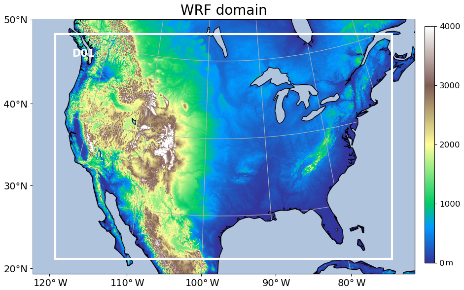
Figure 1Domain and terrain height (m) of the WRF-Chem simulation with 350×290 grid cells and a horizontal resolution of 12 km.
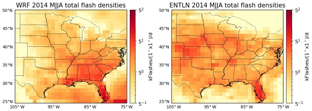
Figure 2Comparison between total flash densities from ENTLN and WRF-Chem during MJJA 2014.
2.4 Method for deriving AMF
The V near convection is calculated according to
where S is the OMI-measured tropospheric slant column NO2, and AMF is a customized lightning air mass factor. The concept of AMF was also used in Beirle et al. (2009) to investigate the sensitivity of satellite instruments to freshly produced lightning NOx. In order to estimate LNOx, we define the AMF as the ratio of the “visible” modeled NO2 slant column to the total modeled tropospheric LNOx vertical column (derived from the a priori NO and NO2 profiles, scattering weights, and cloud radiance fraction):
where fr is the cloud radiance fraction (CRF), psurf is the surface pressure, ptp is the tropopause pressure, pcloud is the cloud optical pressure (CP), wclear and wcloudy are respectively the pressure-dependent scattering weights from the TOMRAD lookup table (Bucsela et al., 2013) for clear and cloudy parts, and NO2(p) is the modeled NO2 vertical profile. Details of these standard parameters and calculation methods are given in Laughner et al. (2018). LNOx(p) is the LNOx vertical profile calculated by the difference of vertical profiles between WRF-Chem simulations with and without lightning.
Please note that the CP is a reflectance-weighted pressure retrieved by the collision-induced O2–O2 absorption band near 477 nm (Acarreta et al., 2004; Sneep et al., 2008; Stammes et al., 2008). For a deep convective cloud with lightning, the CP lies below the geometrical cloud top, which is much closer to that detected by thermal infrared sensors, such as CloudSat and the Aqua Moderate Resolution Imaging Spectrometer (MODIS) (Vasilkov et al., 2008; Joiner et al., 2012). Hence, much of the tropospheric NO2 measured by OMI lies inside the cloud rather than above the cloud top. In the following, “above cloud” or “below cloud” is relative to the cloud pressure detected by OMI. The sensitivity study of Beirle et al. (2009) compared the chemical composition from the cloud bottom to that of the cloud top and revealed that a significant fraction of the NO2 within the cloud originating from lightning can be detected by the satellite. This valuable cloud pressure concept has been applied not only in the LNOx research but also in the cloud slicing method of deriving the UT O3 and NOx (Ziemke et al., 2009, 2017; Choi et al., 2014; Strode et al., 2017; Marais et al., 2018). As discussed in Pickering et al. (2016), the ratio of V seen by OMI to V is partly influenced by pcloud. The effects of LNO2 below the cloud will be discussed in Sect. 3.4.
To compare our results with those of Pickering et al. (2016) and Lapierre et al. (2020), we calculate their AMF and AMF, respectively:
where fg is the geometric cloud fraction and LNO2(p) is the modeled LNO2 vertical profile. Besides these AMFs, another AMF called AMF is developed for later comparison.
A full definition list of the used AMFs is shown in Appendix A.
2.5 Procedures for deriving LNOx
V is re-gridded to grids using the constant value method (Kuhlmann et al., 2014). Then, it is analyzed in grid boxes with a minimum of 50 valid grids to minimize the noise. The main procedures of deriving LNOx are as follows.
CRFs (CRF ≥70 %, CRF ≥90 %, and CRF =100 %) and CP ≤650 hPa are various criteria of deep convective clouds for OMI pixels (Ziemke et al., 2009; Choi et al., 2014; Pickering et al., 2016). The effect of different CRFs on the retrieved LNOx is explored in Sect. 3.2. Furthermore, another criterion of cloud fraction (CF) is applied to the WRF-Chem results for the successful simulation of convection. The CF is defined as the maximum cloud fraction calculated by the Xu–Randall method between 350 and 400 hPa (Xu and Randall, 1996; Strode et al., 2017). This atmospheric layer (between 350 and 400 hPa) avoids any biases in the simulation of high clouds. We choose CF ≥40 % suggested by Strode et al. (2017) to determine cloudy or clear for each simulation grid.
Besides cloud properties, a time period and sufficient flashes (or strokes) are required for fresh LNOx to be detected by OMI. The time window (twindow) is the hours prior to the OMI overpass time. twindow is limited to 2.4 h by the mean wind speed at pressure levels 500–100 hPa during OMI overpass time and the square root of the box over the CONUS (Lapierre et al., 2020). Meanwhile, 2400 flashes per box and 8160 strokes per box per 2.4 h time window are chosen as sufficient for detecting LNOx (Lapierre et al., 2020). These criteria will result in a low bias in the PE results, as Bucsela et al. (2019) found that the PE is larger at small flash rates, which are discarded here. Since our study focuses on developing a new AMF and compares results with other works using similar lightning thresholds (Lapierre et al., 2020; Pickering et al., 2016), we will only discuss results based on the strict criteria in the main text. For comparisons between the criterion of 2400 flashes per box and that of one flash per box, scatter diagrams using different lightning criteria are presented in Appendix B.
To ensure that lightning flashes are simulated successfully by WRF-Chem, the threshold of simulated total lightning flashes (TL) per box is set to 1000, which is fewer than that used by the ENTLN lightning observation, considering the uncertainty of lightning parameterization. In view of other NO2 sources in addition to LNO2, the ratio of modeled lightning NO2 above cloud (LNO2Vis) to modeled NO2 above cloud (NO2Vis) is defined to check whether enough LNO2 can be detected by OMI. The ratio ≥50 % indicates that more than half of the NOx above the cloud must have an LNOx source.
Finally, the NO2 lifetime due to oxidation should be taken into account. As estimated by Nault et al. (2017), the lifetime (τ) of NO2 in the near field of convections is ∼ 3 h. The initial value of NO2 is solved by Eq. (6) as
where NO2(0) is the moles of NO2 emitted at time t=0, NO2(OMI) is the moles of NO2 measured at the OMI overpass time, and 0.5t is the half cross grid time, which is 1.2 h, assuming that lightning occurred at the center of each box. For each grid box, the mean LNOx vertical column is obtained by averaging V values from all regridded pixels in the box. This mean value is converted to moles of LNOx using the dimensions of the grid box. Two methods are applied to estimate the seasonal mean LNO2 per flash, LNOx per flash, LNO2 per stroke, and LNOx per stroke:
-
summation method, dividing the sum of LNOx by the sum of flashes (or strokes) in each box in MJJA 2014;
-
linear regression method, applying the linear regression to daily mean values of LNOx and flashes (or strokes).
3.1 Criteria determination
To determine the suitable criteria from the conditions defined in Sect. 2.5, six different combinations are defined (Table 1) and applied to the original data with a linear regression method (Table 2).
Table 1Definitions of the abbreviations for the criteria used in this study.
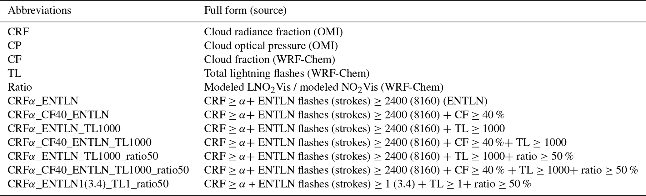
α has three options: 70 %, 90 %, or 100 %.
Table 2LNOx production efficiencies for different combinations of criteria defined in Table 1.
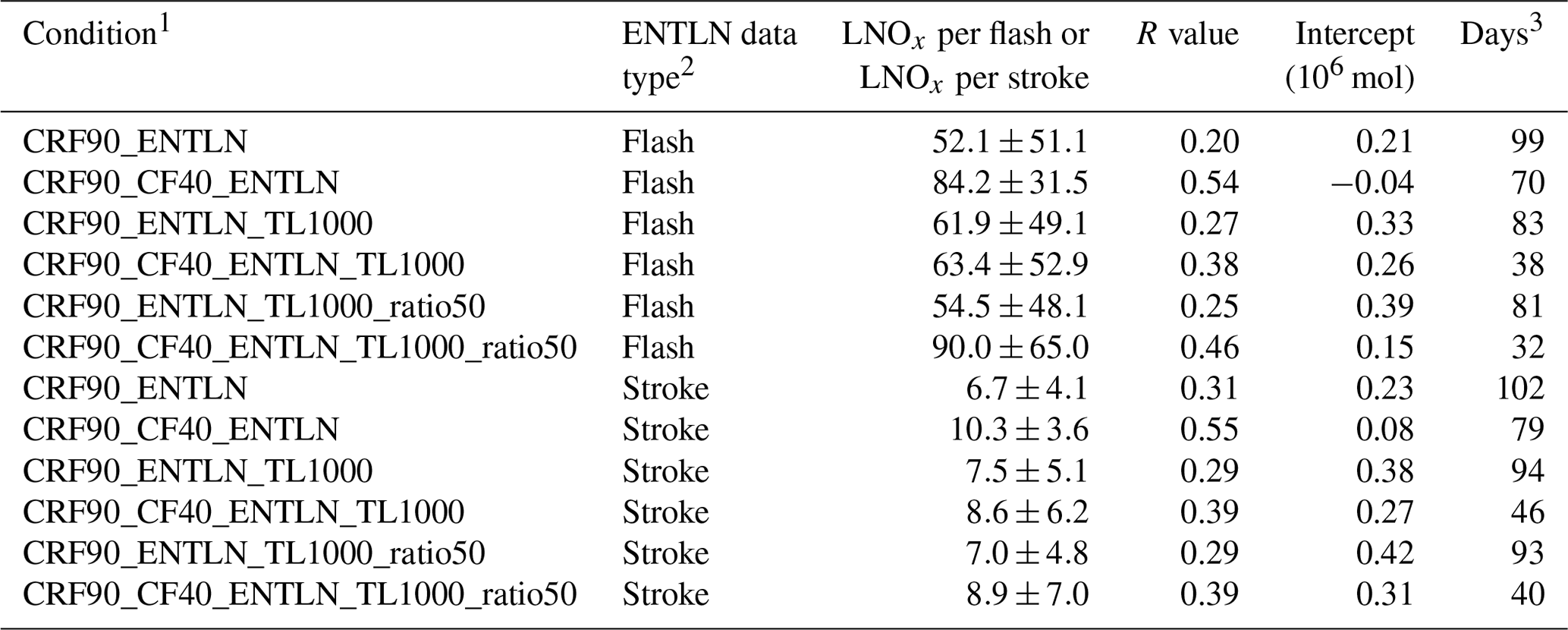
1 These conditions are defined in Table 1. 2 The thresholds of ENTLN data are 2400 flashes per box and 8160 strokes per box during the period of 2.4 h before OMI overpass time. 3 The number of valid days with specific criteria in MJJA 2014.
A daily search of the NO2 product for coincident ENTLN flash (stroke) data results in 99 (102) valid days under the CRF90_ENTLN condition. Taking the flash-type ENTLN data as an example, the number of valid days decreases from 99 to 81 under the CRF90_ENTLN_TL1000_ratio50 condition, while LNOx per flash increases from 52.1±51.1 to 54.5±48.1 mol per flash. The result is almost the same as that under the CRF90_ENTLN_TL1000 condition, which is without the condition of more than half of the above-cloud NOx having an LNOx source. Although this indicates the criterion of TL works well, it is better to include the ratio criterion in case there are some exceptions in the different AMF methods. Since CF ≥40 % leads to a sharp loss of valid numbers and production, it is not a suitable criterion. Instead the CRF criteria are used. Finally, coincident ENTLN data, TL ≥1000, and ratio ≥50 % are chosen as the thresholds to explore the effects of three different CRF conditions (CRF ≥70 %, CRF ≥90 %, and CRF =100 %) on LNOx production (Table 3). Apart from the fewer valid days under higher CRF conditions (CRF ≥90 % and CRF =100 %), LNOx per flash increases from 35.7±36.8 to 54.5 ± 48.1 mol per flash and decreases again to 20.8±37.4 mol per flash while LNOx per stroke enhances from 4.1±3.9 to 7.0±4.8 mol per stroke and drops again to 2.6±4.0 mol per stroke (Table 3), as the CRF criterion increases from 70 % to 90 % and to 100 %. When the CRF increases from 90 % to 100 %, the LNOx PE decreases because of the higher lightning density with less LNOx (not shown). The increment of LNOx PE caused by the CRF increase from 70 % to 90 % is opposite to the result of Pickering et al. (2016). This is an effect of the consideration of NO2 contamination transported from the boundary layer in our method. Although enhanced NOx is often observed in regions with CRF >70 % (Pickering et al., 2016), the following analysis will be based on the criterion of CRF ≥90 % considering the contamination by low and midlevel NO2 and comparisons with the results of Pickering et al. (2016) and Lapierre et al. (2020).
Table 3LNOx production efficiencies for different thresholds of CRF with coincident ENTLN data, TL ≥1000, and ratio ≥50 %.
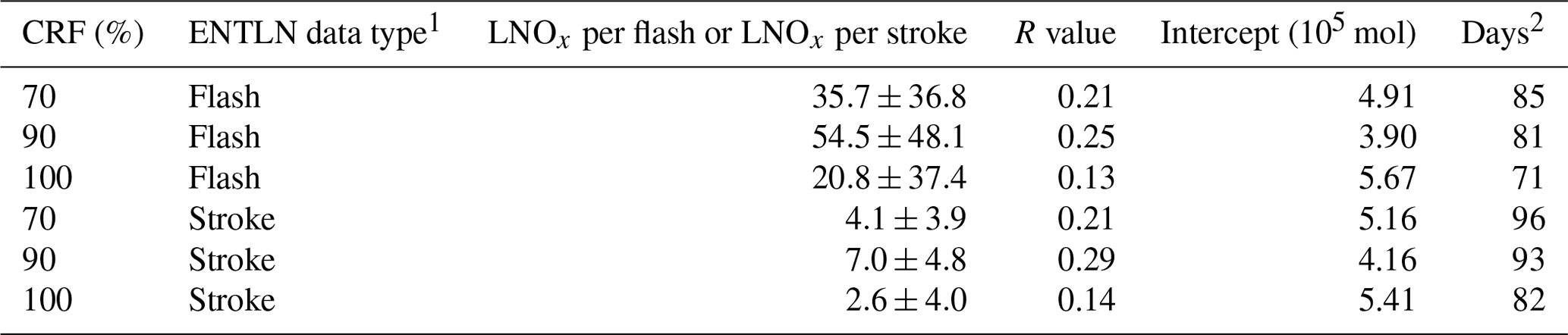
1 The thresholds of ENTLN data are 2400 flashes per box and 8160 strokes per box during the period of 2.4 h before OMI overpass time. 2 The number of valid days with specific criteria in MJJA 2014.
3.2 Comparison of LNOx production based on different AMFs
Lapierre et al. (2020) derived LNO2 production based on the BEHR NO2 product. In order for our results to be comparable with those of Pickering et al. (2016) and Lapierre et al. (2020), we choose NO2 instead of NOx to derive production per flash (production efficiency, PE). In Fig. 3, time series of NO2Vis, LNO2Vis, LNO2, and LNO2Clean production per day over CONUS are plotted for MJJA 2014 with the criterion of CRF ≥90 % and a flash threshold of 2400 flashes per 2.4 h. LNO2 PEs are mostly in the range from 20 to 80 mol per flash. LNO2Vis PEs are smaller than LNO2 PEs, which contain LNO2 below clouds. The simulation of GMI in Pickering et al. (2016) indicated that 25 %–30 % of the LNOx column lies below the CP, while the ratio in our WRF-Chem simulation is 56±20 %. The effect of cloud properties on LNOx PE will be discussed in more detail in Sect. 3.4. Generally, the order of estimated daily PEs is LNO2Clean > LNO2 > NO2Vis > LNO2Vis. The percent difference in the estimated PE (ΔPE) between NO2Vis and LNO2Vis indicates a certain amount of background NO2 exists above clouds. Overall, the tendency of that ΔPE is consistent with another ΔPE between NO2Vis and LNO2Clean. When the region is highly polluted (ΔPE between NO2Vis and LNO2Vis is larger than 200 %), PEs based on NO2Vis and LNO2Clean are significantly overestimated. In other words, NO2Vis and LNO2Clean are more sensitive to background NO2. The extent of the overestimation of NO2Vis is larger than that of LNO2Clean in highly polluted regions, while it is usually opposite in most regions.
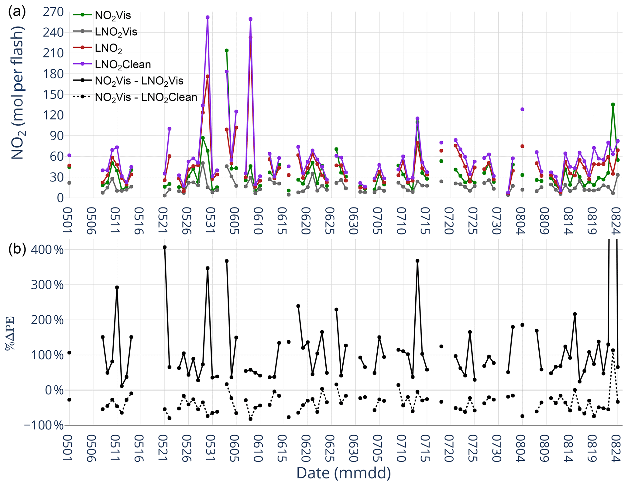
Figure 3(a) Time series of NO2Vis, LNO2Vis, LNO2, and LNO2Clean production per day over the CONUS for MJJA 2014 with CRF ≥90 % and a flash threshold of 2400 flashes per 2.4 h. (b) Time series of the percent differences between NO2Vis and LNO2Vis and the percent differences between NO2Vis and LNO2Clean with CRF ≥90 %. The value of the black dot on 23 August (not shown) is 1958 %.
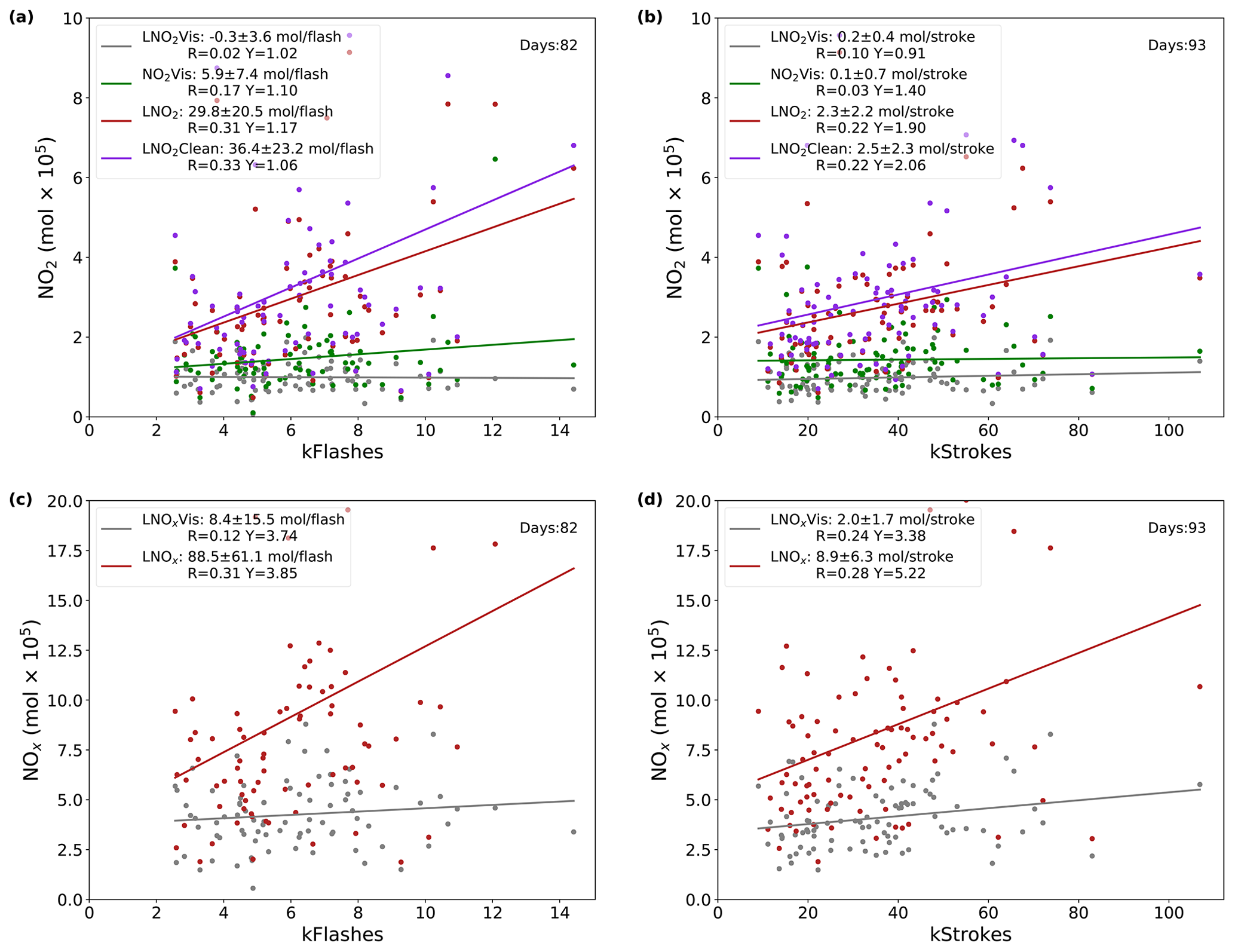
Figure 4 shows the linear regression for ENTLN data versus NO2Vis, LNO2Vis, LNO2, and LNO2Clean with the same criteria as shown in Fig. 3. LNO2Clean PE (the largest slope) is 25.2±22.3 mol NO2 per flash with a correlation of 0.25 and 2.3±2.1 mol NO2 per stroke with a correlation of 0.22. As shown in Fig. 3, positive percent differences between NO2Vis PE and LNO2Clean PE occur much less often than negative differences. As a result, NO2Vis PE (17.1±17.2 mol NO2 per flash and 0.4±1.0 mol NO2 per stroke) is smaller than LNO2Clean PE using the linear regression method.
In order to compare our result with that of Lapierre et al. (2020), we tried to remove the CP ≤650 hPa, TL ≥1000, and ratio ≥50 % conditions from criteria. But, our result based on daily summed NO2Vis values (3.8±0.5 mol per stroke) is still larger than the value of 1.6± 0.1 mol per stroke mentioned in Lapierre et al. (2020). This may be caused by the different version of the BEHR algorithm, as Lapierre et al. (2020) used BEHR v3.0A and our algorithm is based on BEHR v3.0B (Laughner et al., 2019). The input of S in both versions is from the NASA standard product v3, and the major improvements of BEHR v3.0B are listed below.
-
The profile (v3.0B) closest to the OMI overpass time was selected instead of the last profile (v3.0A) before the OMI overpass.
-
The AMF uses a variable tropopause height as opposed to the fixed 200 hPa tropopause.
-
The surface pressure is now calculated according to Zhou et al. (2009).
The detailed log of changes is available at https://github.com/CohenBerkeleyLab/BEHR-core/blob/master/Documentation/Changelog.txt (last access: 20 March 2020). Note that Lapierre et al. (2020) used the monthly NO2 profile. While the daily profile is used in our study and the interval of our outputs from WRF-Chem is 30 min, which is more frequent than 1 h in the BEHR daily product, the AMF could be affected by different NO2 profiles. In view of these factors, we compare different methods based on our data to minimize these effects.
Meanwhile, LNO2 PE (18.7±18.1 mol per flash and 2.1±1.8 mol per stroke) is between LNO2Clean PE and NO2Vis PE, which coincides with the daily results in Fig. 3. Furthermore, the LNOx PE based on the linear regression of daily summed values, the same method used in Pickering et al. (2016), is 114.8±18.2 mol per flash (or 17.8±2.9 mol per stroke), which is larger than 91 mol per flash in Pickering et al. (2016), possibly due to the differences in geographic location, lightning data, and chemistry model.
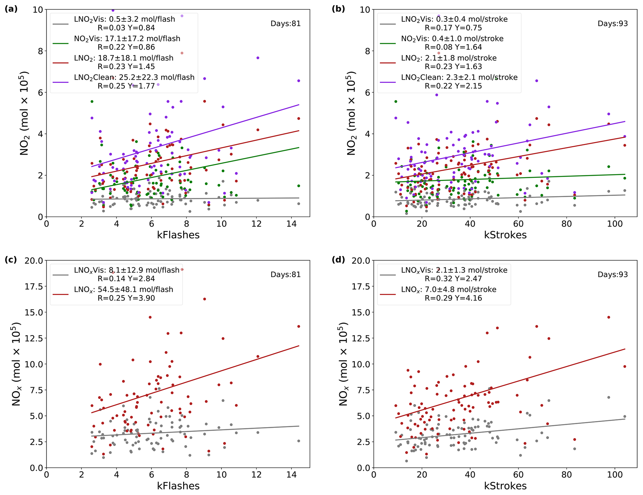
Figure 4(a) Daily NO2Vis, LNO2Vis, LNO2, and LNO2Clean versus ENTLN total flash data. (b) Same as (a) but for strokes. (c) Daily LNOxVis and LNOx versus total flashes. (d) Same as (c) but for strokes.
The mean and standard deviation of LNO2 PE under CRF ≥90 % using the summation method is 46.2±35.1 mol per flash and 9.9±8.1 mol per stroke, while LNOx PE is 125.6±95.9 mol per flash and 26.7±21.6 mol per stroke (Fig. 5). The LNO2 PE and LNOx PE are both higher in the southeast US (denoted by the red box in Fig. 5, 25–37∘ N, 75–95∘ W), consistent with Lapierre et al. (2020) and Bucsela et al. (2019). Compared with Fig. 3, Fig. 6a and b present some large differences between NO2Vis PE and LNO2Vis PE, which are consistent with what we expect for polluted regions. Meanwhile, the differences between LNO2 PE and NO2Vis PE depend on background NO2, the strength of updraft, and the profile. The negative differences are caused by background NO2 carried by the updraft while parts of the below-cloud LNO2 result in LNO2 PE higher than NO2Vis PE (Fig. 6c). Figure 6d shows that the ratio of LNO2Vis to LNO2 ranges from 10 % to 80 %. This may be caused by the height of the clouds and the profile of LNO2. If the CP is near 300 hPa, the ratio should be smaller because of the coverage of clouds. While peaks of the LNO2 profile are below the CP, the ratio would also be smaller. Therefore, a better understanding of the LNO2 profile and LNOx below clouds is required.

Figure 5(a, c) Maps of gridded values of mean LNOx and LNO2 production per flash with CRF ≥90 % for MJJA 2014. (b, d) Same as (a) and (c) except for strokes. The southeastern US is denoted by the red box in panels (a)–(d).
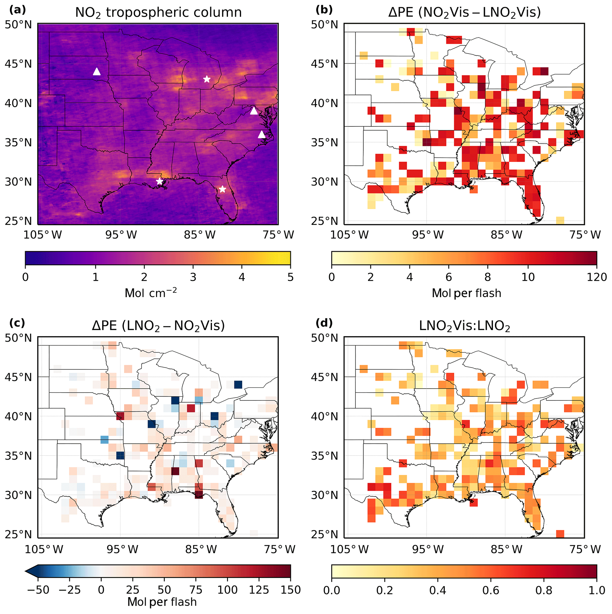
Figure 6(a) Mean (MJJA 2014) NO2 tropospheric column. Polluted cities are denoted by stars (Lansing, New Orleans, and Orlando) while clean cities are denoted by triangles (Huron, Charles Town, and Tarboro). (b) The differences of the estimated mean production efficiency between NO2Vis and LNO2Vis with CRF ≥90 %. (c) The same differences as (b) but between LNO2 and NO2Vis. (d)The ratio of LNO2Vis to LNO2.
3.3 Effects of tropospheric background on LNOx production
With respect to the LNO2 production, the patterns in Fig. 6 indicate the improvement of our approach is different in polluted and clean regions. To simplify the quantification, we select six grids with similar NO2 profiles (∼100 pptv) above the cloud with CRF =100 %. These grid boxes contain the polluted and clean cities denoted by stars and triangles in Fig. 6a, respectively. Then, the differences between AMFs are dependent on fewer parameters.
Figure 7 compares the mean profiles of NO2, background NO2 and background NO2 ratio in polluted and clean grids. Generally, the profiles of the ratio of background NO2 to total NO2 are C shaped because UT LNO2 concentrations are higher than UT background NO2 concentrations. However, the ratio profile in Fig. 7e has one peak between the cloud pressure and tropopause as background NO2 increases and LNO2 decreases. Besides, the percentage of UT background NO2 in polluted regions is steady and higher than that in clean regions.
Table 4 presents the relative changes among three methods in six cities. The difference between AMF (Eq. 7) and AMF (Eq. 9) is the numerator: and . When the ratio of LNO2 is higher or the region is cleaner, the relative difference is smaller (e.g. 5.0 %–12.0 %, Fig. 7d–f). The largest relative difference (46.3 %) occurs when the ratio of background NO2 is continuously high in the UT (Fig. 7c). As a result, our approach is less sensitive to background NO2 and more suitable for convective cases over polluted locations. In contrast, production estimated by our method is larger than that based on NO2Vis due to the LNO2 below the cloud. When the cloud is higher, in particular the peak of the LNO profile is lower than the cloud (Fig. 7b). The relative difference is larger (121.2 %) because more LNO2 can not be included in the NO2Vis, which has been discussed in Sect. 3.2. The relative change between AMF (Eq. 9) and AMF (Eq. 8) depends on , which is also affected by cloud, not the background NO2. The largest relative change (153.8 %) occurs at New Orleans, which has the lowest cloud pressure and consequently the smallest visible column.
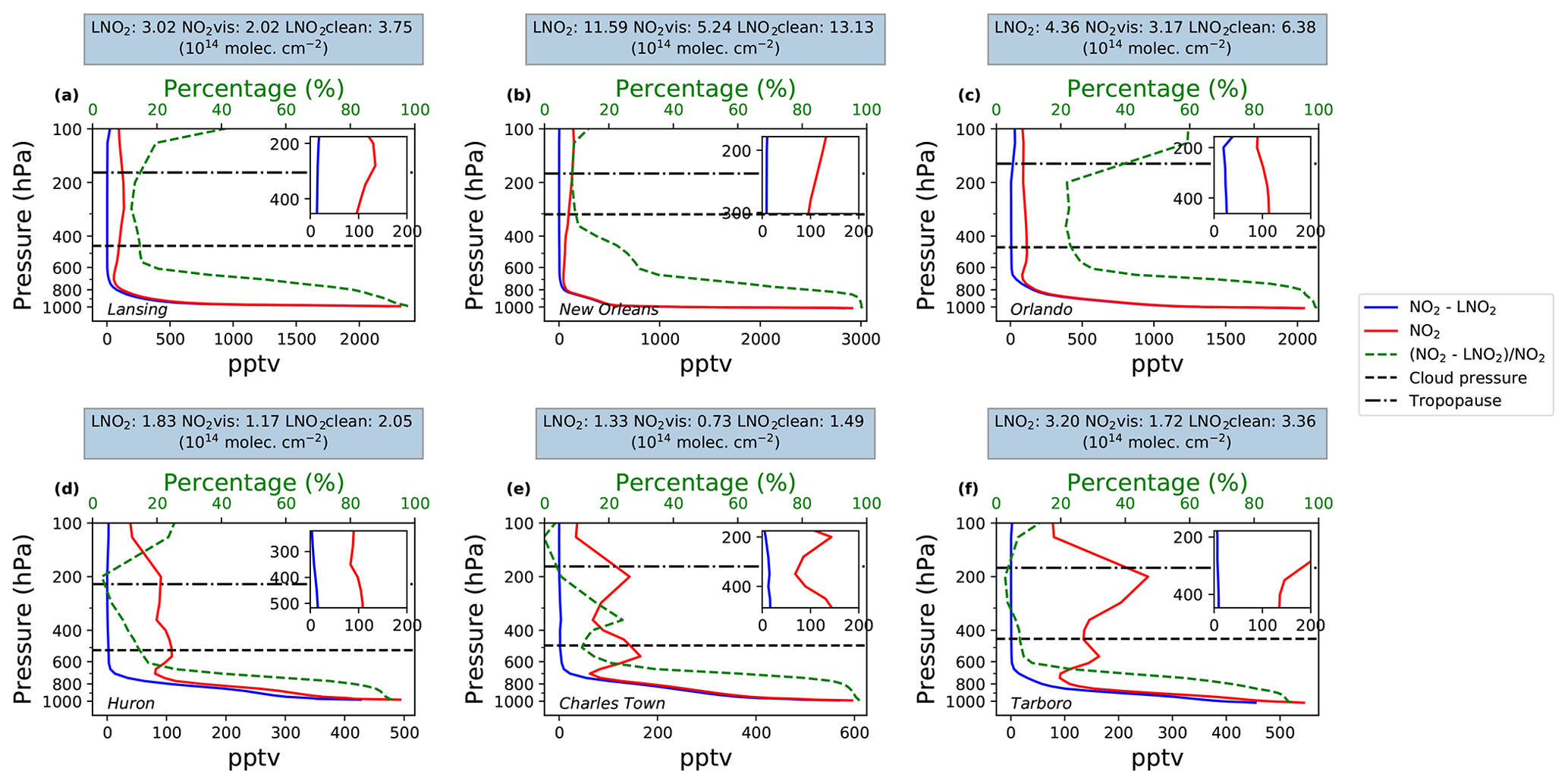
Figure 7Comparisons of mean WRF-Chem NO2 and background NO2 profiles in six grids with CRF ≥100 % on specific days during MJJA 2014. The (a), (b), and (c) data are selected from polluted regions (stars in Fig. 6a) while the (d), (e), and (f) data are from clean regions (triangles in Fig. 6a). The green dashed lines are the mean ratio profiles of background NO2 to total NO2. The zoomed figures show the profiles from the cloud pressure to the tropopause. The titles present the mean productions based on three different methods mentioned in Sect. 2.4.
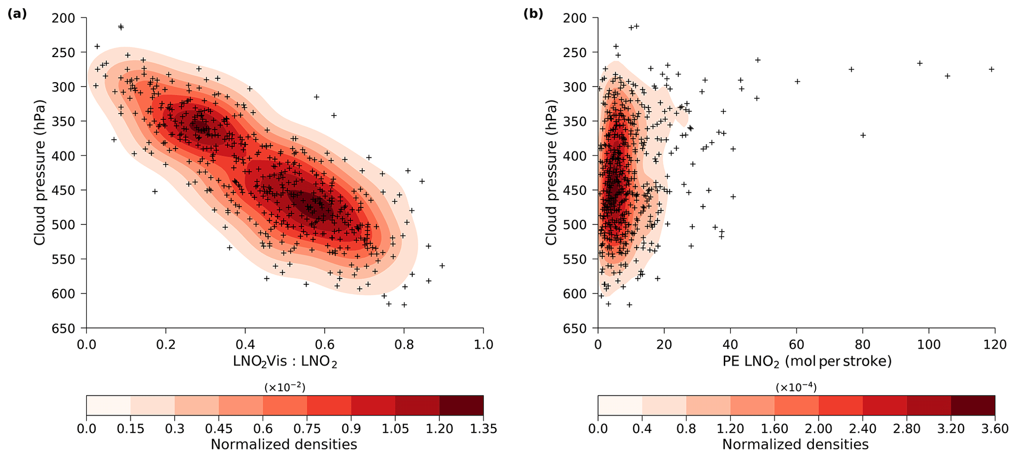
Figure 8Kernel density estimation of the (a) daily ratio of LNO2Vis to LNO2 and (b) daily LNO2 production efficiency versus the daily cloud pressure measured by OMI with CRF ≥90 % for MJJA 2014. The kernel density estimation was generated by kdeplot in the Python package named seaborn.
3.4 Effects of cloud and LNOx parameterization on LNOx production
Figure 8a presents the daily distribution of CP and the ratio of LNO2Vis to LNO2 during MJJA 2014 with the criteria defined in Sect. 3.1 under CRF ≥90 %. Since the ratio of LNO2Vis to LNO2 decreases from 0.8 to 0.2 as the cloud pressure decreases from 600 to 300 hPa, NO2Vis PE is smaller than LNO2 PE in relatively clean areas as shown in Fig. 4. Apart from LNO2Vis, the LNO2 PE is also affected by CP. For LNO2 PEs larger than 30 mol per stroke, the CPs are all smaller than 550 hPa (Fig. 8b). However, smaller LNO2 PEs (<30 mol per stroke) occur on all levels between 650 and 200 hPa. Because of the limited number of large LNO2 PEs and lightning data, we cannot derive the relationship between LNO2 PE and cloud pressure or other lightning properties at this stage. Because the CP only represents the development of clouds, the vertical structure of flashes can not be derived from the CP values only. As discussed in several previous studies, the flash channel length varies and depends on the environmental conditions (Carey et al., 2016; Mecikalski and Carey, 2017; Fuchs and Rutledge, 2018). Davis et al. (2019) compared two kinds of flash: normal flashes and anomalous flashes. Because updrafts are stronger and flash rates are higher in anomalous storms, UT LNOx concentrations are larger in anomalous than normal polarity storms. In general, normal flashes are coupled with an upper-level positive charge region and a midlevel negative charge region, while anomalous flashes are opposite (Williams, 1989). It is not straightforward to estimate the error resulting from the vertical distribution of LNOx. There are mainly two methods of distributing LNOx in models: LNOx profiles (postconvection) in which LNOx has already been redistributed by convective transport and LNOx production profiles (preconvection) made before the redistribution of convective transport (Allen et al., 2012; Luo et al., 2017). However, given the similarity of results compared to other LNOx studies, we believe that our results based on postconvective LNOx profiles are sufficient for estimating average LNOx production.
Table 4The percent changes in the estimated production when using different methods based on the same a priori profiles.
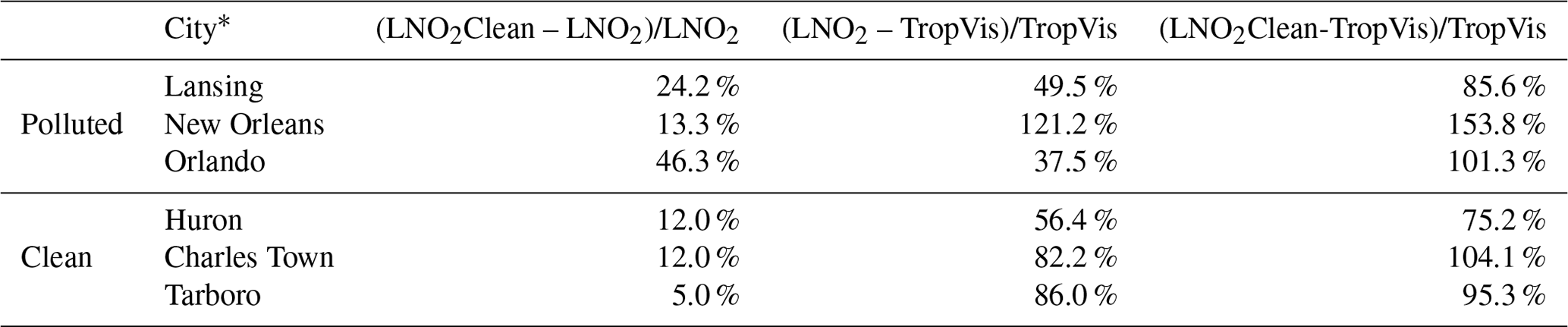
* Locations are denoted in Fig. 6a.
The LNO production settings in WRF-Chem varied in different studies. Zhao et al. (2009) set a NOx production rate of 250 mol NO per flash in a regional-scale model, while Bela et al. (2016) chose 330 mol NO per flash used by Barth et al. (2012). Wang et al. (2015) assumed approximately 500 mol NO per flash, which was derived by a cloud-scale chemical transport model and in-cloud aircraft observations (Ott et al., 2010). To illustrate the impact of LNOx parameterization on LNOx estimation, we apply another WRF-Chem NO2 profile setting (2× base flash rate, 500 mol NO per flash, hereinafter referred to as “2×500 mol NO per flash”) to a priori profiles and evaluate the changes in AMF, AMF, LNO2 PE, and LNOx PE. For the linear regression method (Fig. 9), LNO2 PE is 29.8±20.5 mol per flash, which is 59.4 % larger than the basic one (18.7±18.1 mol per flash). Meanwhile, LNOx PE (increasing from 54.5±48.1 mol per flash to 88.5±61.1 mol per flash) also depends on the configuration of LNO production in WRF-Chem. The comparison between Figs. 4 and 9 shows that LNO2Clean PE and LNO2 PE are more similar while LNO2 PE and NO2Vis PE present the same tendency. It remains unclear as to whether the NO–NO2–O3 cycle or other LNOx reservoirs account for the increment of LNOx PE. This would need detailed source analysis in WRF-Chem and is beyond the scope of this study.
Figure 10 shows the average percentage changes in AMF, AMF, LNO2, and LNOx between retrievals using profiles based on 1×200 and 2×500 mol NO per flash. These results were obtained by averaging data over MJJA 2014 based on the method described in Sect. 2.5 with the criterion of CRF ≥90 %. The effects on LNO2 and LNOx retrieval from increasing LNO profile values show mostly the same tendency: smaller AMF and AMF lead to larger LNO2 and LNOx, but the changes are regionally dependent. This is caused by the nonlinear calculation of AMF and AMF. As the contribution of LNO2 increases, both the numerator and denominator of Eq. (2) increase. Note that the LNO2 accounts for a fraction of NO2 above the clouds. The magnitude of an increasing denominator could be different than that of an increasing numerator, resulting in a different effect on the AMF and AMF. As mentioned in Zhu et al. (2019), the lightning densities in the southeast US might be overestimated using the 2×500 mol NO per flash setting and the same lightning parameterization as ours. Fortunately, the AMFs and estimated LNO2 change little in that region. Because the southeast US has the highest flash density (Fig. 2), the NO2 in the numerator of AMF is dominated by LNO2. Both the SCD and VCD will increase when the model uses higher LNO2. In other words, the sensitivity to the LNO setting decreases and the relative distribution of LNO2 matters.
Figure 11 shows the comparison of the mean LNO and LNO2 profiles in two specific regions where the 2×500 mol NO per flash setting leads to lower and higher LNO2 PEs, respectively. The first one (Fig. 11a) is the region (36–37∘ N, 89–90∘ W) containing the minimal negative percent change in LNO2 (Fig. 10c). The second one (31–32∘ N, 97–98∘ W), Fig. 11b, has the largest positive percent change in LNO2 (Fig. 10c). Although the relative distributions of mean LNO and LNO2 profiles are similar in both regions, the magnitude differs by a factor of 10. This phenomenon implies that the performance of lightning parameterization in WRF-Chem is regionally dependent, and an unrealistic profile could appear in the UT. Although this sensitivity analysis is false in some regions, it allows the calculation of an upper limit on the NO2 due to LNO and LNO2 profiles. As discussed in Laughner and Cohen (2017), the scattering weights are uniform under cloudy conditions and the sensitivity of NO2 is nearly constant with different pressure levels because of the high albedo. However, the relative distribution of LNO2 within the UT should be taken carefully into consideration. If the LNO2∕NO2 above the cloud is large enough (Fig. 11a), the AMF is largely determined by the ratio of LNO2Vis to LNO2, which is related to the relative distribution. When the condition of high LNO2∕NO2 is not met, both relative distribution and ratio are important (Fig. 11b).

Figure 10Average percent differences in (a) AMF, (b) AMF, (c) LNO2, and (d) LNOx with CRF ≥90 % over MJJA 2014. Differences between profiles are generated by 2×500 and 1×200 mol NO per flash.
To clarify this, we applied the same sensitivity test of different simulating LNO amounts for all four methods mentioned in Sect. 2.4: LNO2, LNO2Vis, LNO2Clean, and NO2Vis (Fig. 12). Note that the threshold for CRF is set to 100 % to simplify Eq. (2) to Eq. (7). The overall differences of LNO2Clean and NO2Vis are smaller than those of LNO2 and LNO2Vis. Comparing the numerator and denominator in the equations, it is clear why the impact of different simulating LNO amounts is smaller in Fig. 12c and d. For LNO2Clean and NO2Vis, both the SCD and VCD will increase (decrease) when more (less) LNO2 or NO2 presents. The difference between Fig. 12a and b is the denominator: the total tropospheric LNO2 vertical column and visible LNO2 vertical column, respectively. As a result, the negative values in Fig. 12a are caused by the part of LNO2 below the cloud. The uncertainty of retrieved LNO2 and LNOx PEs is driven by this error, and we conservatively estimate this to be ±13 % and ±25 %, respectively.
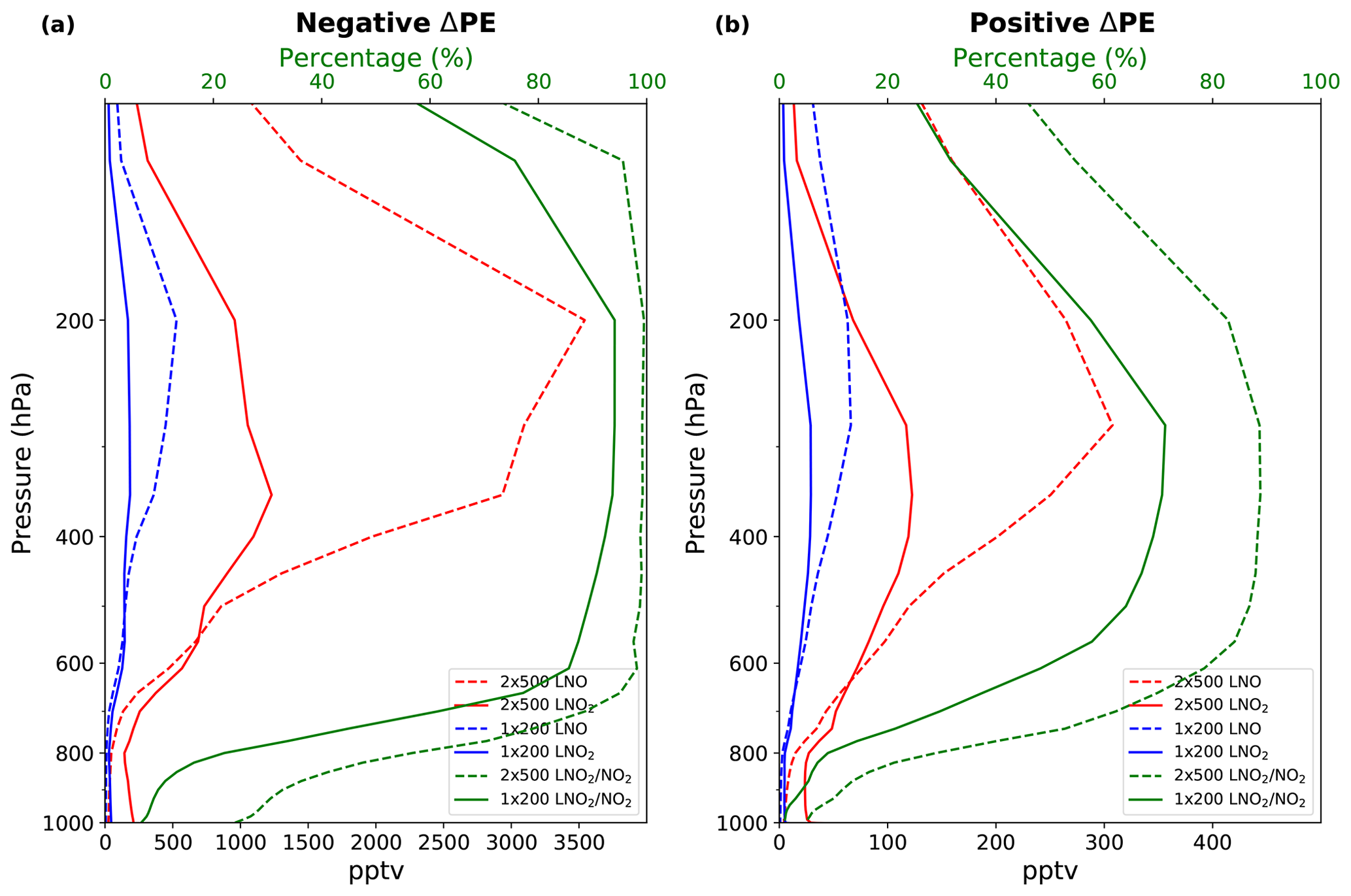
Figure 11LNO and LNO2 profiles with different LNO settings in (a) the region containing the minimal negative percent change in LNO2 and (b) the region containing the largest positive percent change in LNO2 when the LNO setting is changed from 1×200 to 2×500 mol NO per flash, averaged over MJJA 2014. The profiles using 1×200 (2×500) mol NO per flash are shown in blue (red) lines. Solid (dashed) green lines are the mean ratio of LNO2 to NO2 with 1×200 (2×500) mol NO per flash.
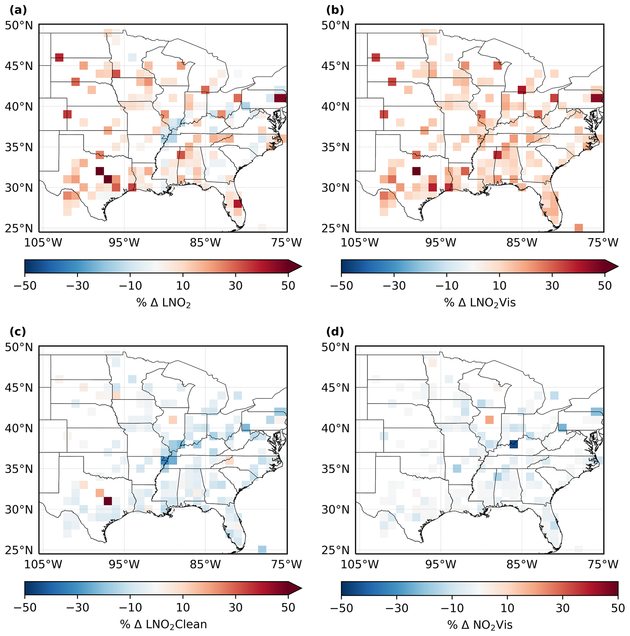
Figure 12Average percent differences in (a) LNO2, (b) LNO2Vis, (c) LNO2Clean, and (d) NO2Vis with CRF =100 % over MJJA 2014.
The uncertainties of the LNO2 and LNOx PEs are estimated following Pickering et al. (2016), Allen et al. (2019), Bucsela et al. (2019), Laughner et al. (2019) and Lapierre et al. (2020). We determine the uncertainty due to BEHR tropopause pressure, cloud radiance fraction, cloud pressure, surface pressure, surface reflectivity, profile shape, profile location, Vstrat, the detection efficiency of lightning, twindow, and LNO2 lifetime numerically by perturbing each parameter in turn and re-retrieving the LNO2 and LNOx with the perturbed values (Table 5).
Table 5Uncertainties for the estimation of LNO2 per flash, LNOx per flash, LNO2 per stroke, and LNOx per stroke.
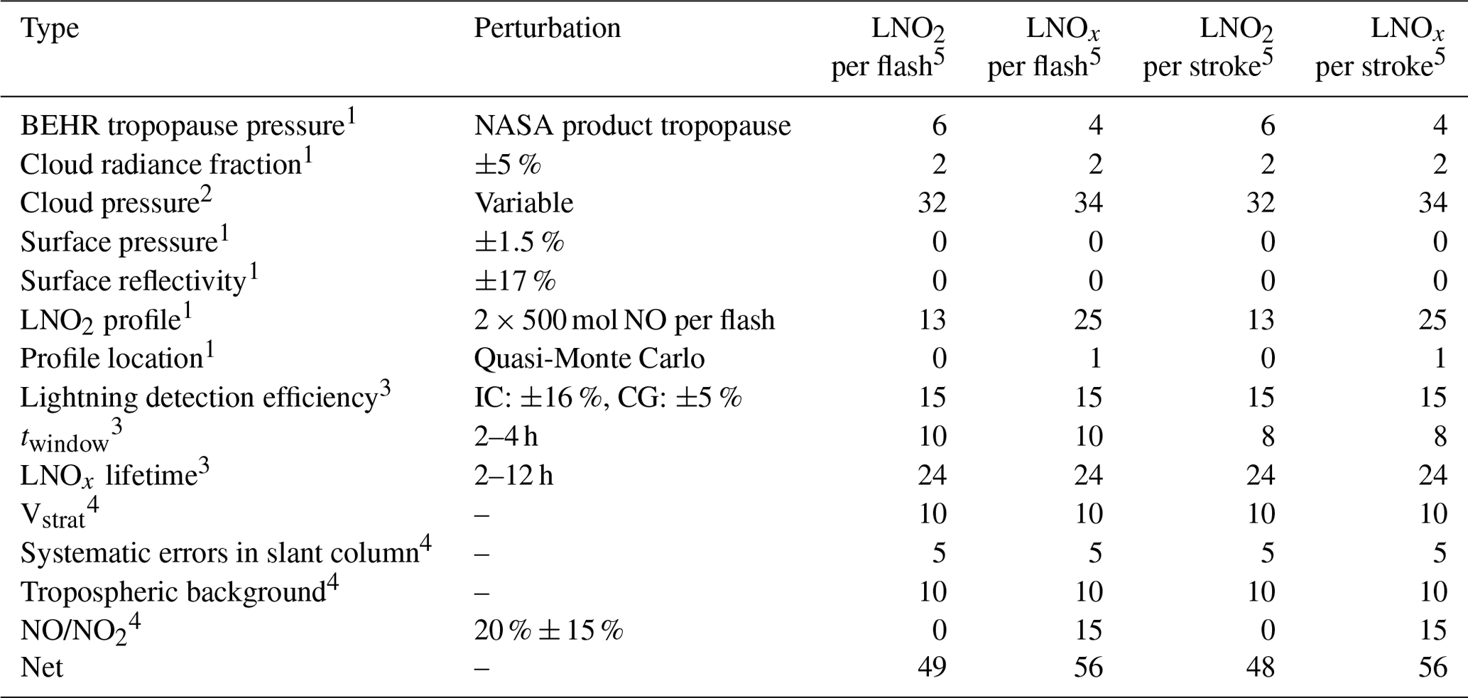
PEuncertainty= (Errorrising perturbed value - Errorlowering perturbed value)/2, where Errorperturbed value= (PE perturbed value – PEoriginal value)/PEoriginal value. 1 Laughner et al. (2019). 2 Acarreta et al. (2004). 3 Lapierre et al. (2020). 4 Allen et al. (2019) and Bucsela et al. (2019). 5 Uncertainty (%).
The GEOS-5 monthly tropopause pressure, which is consistent with the NASA standard product, is applied instead of the variable WRF tropopause height to evaluate the uncertainty (6 % for LNO2 PE and 4 % for LNOx PE) caused by the BEHR tropopause pressure. The cloud pressure bias is given as a function of cloud pressure and fraction by Acarreta et al. (2004), implying an uncertainty of 32 %, the most likely uncertainty in the production analysis, for LNO2 PE and 34 % for LNOx PE. The resolution of GLOBE terrain height data is much higher than the OMI pixel, and a fixed scale height is assumed in the BEHR algorithm. As a result, Laughner et al. (2019) compared the average WRF surface pressures to the GLOBE surface pressures and arrived at the largest bias of 1.5 %. Based on the largest bias, we vary the surface pressure (limited to less than 1020 hPa), and the uncertainty can be neglected.
The error in cloud radiance fraction is transformed from cloud fraction using
where fr is the cloud radiance fraction, fg is the cloud fraction, and fg,pix is the cloud fraction of a specific pixel. We calculate under fg,pix by the relationship between all binned fr and fg with the increment of 0.05 for the each specific OMI orbit. Considering the relationship, the error in cloud fraction is converted to an error in cloud radiance fraction of 2 % for the LNO2 and LNOx PEs.
The accuracy of the 500 m MODIS albedo product is usually within 5 % of albedo observations at the validation sites, and those exceptions with low-quality flags have been found to be primarily within 10 % of the field data (Schaaf et al., 2011). Since we use the bidirectional reflectance distribution function (BRDF) data directly, rather than including a radiative transfer model, 14 % Lambertian equivalent reflectivity (LER) error and 10 % uncertainty are combined to get a perturbation of 17 % (Laughner et al., 2019). The uncertainty due to surface reflectivity can be neglected with the 17 % perturbation.
As discussed at the end of Sect. 3.4, another setting of LNO2 (2×500 mol NO per flash) is applied to determine the uncertainty of the lightning parameterization and the vertical distribution of LNO in WRF-Chem. Differences between the two profiles lead to an uncertainty of 13 % and 25 % in the resulting PEs of LNO2 and LNOx. Another sensitivity test allows each pixel to shift by −0.2, 0, or +0.2 ∘ in the directions of longitude and latitude, taking advantage of the high-resolution profile location in WRF-Chem. The resulting uncertainty of LNOx PE is 1 %, including the error of transport and chemistry by shifting pixels.
Compared to the NASA standard product v2, Krotkov et al. (2017) demonstrated that the noise in Vstrat is 1×1014 cm−2. Errors in polluted regions can be slightly larger than this value, while errors in the cleanest areas are typically significantly smaller (Bucsela et al., 2013). We estimated the uncertainty of the Vstrat component and the slant column errors to be 10 % and 5 %, respectively, following Allen et al. (2019).
Based on the standard deviation of the detection efficiency estimation over the CONUS relative to LIS, ENTLN detection efficiency uncertainties are ± 16 % for total and IC flashes and strokes. Due to the high detection efficiency of CG over the CONUS, the uncertainty is estimated to be ±5 % (Lapierre et al., 2020). It is found that the resulting uncertainty of detection efficiency is 15 % in the production analysis. We have used the twindow of 2.4 h for counting ENTLN flashes and strokes to analyze LNO2 and LNOx production. Because twindow derived from the ERA5 reanalysis can not represent the variable wind speeds, a sensitivity test is performed which yields an uncertainty of 10 % for production per flash and 8 % for production per stroke using twindow of 2 and 4 h. Meanwhile, the lifetime of UT NOx ranges from 2 to 12 h depending on the convective location, the methyl peroxy nitrate and alkyl, and multifunctional nitrates (Nault et al., 2017). The lifetime (τ) of NO2 in Eq. (6) is replaced by 2 and 12 h to determine the uncertainty as 24 % due to lifetime. This is comparable with the uncertainty (25 %) caused by lightning parameterization for the LNOx type.
Recent studies revealed that the modeled NO∕NO2 ratio departs from the data in the SEAC4RS aircraft campaign (Travis et al., 2016; Silvern et al., 2018). Silvern et al. (2018) attributed this to the positive interference on the NO2 measurements or errors in the cold-temperature photochemical reaction rate. We assign a 20 % bias with ±15 % uncertainty to this error considering the possible positive NO2 measurement interferences (Allen et al., 2019; Bucsela et al., 2019) and estimate the uncertainty to be 15 % for LNOx PE.
In addition, the estimation of LNOx PE also depends on the tropospheric background NO2. In our method, the main factors affecting this factor are the emissions inventory and the amount of transported NO2. For the emissions inventory, the sources of uncertainty are assumptions, methods, input data, and calculation errors. As a result, the uncertainties for different species or pollutants related to NO2 are different and the U.S. EPA also does not publish the quantified uncertainty measures because the parties that submit emissions estimates to the U.S. EPA are not asked to include quantitative uncertainty measurements or estimates (EPA, 2015). For the simulated convective transport, Li et al. (2018) compared the cloud-resolving simulations with these based on convective parameterization and pointed out that the convective transport was weaker in the parameterization. But, we believe that the ratio condition (LNO2Vis/NO2Vis ≥50 %) should reduce these two kinds of uncertainty, and we assume an uncertainty of 10 %, which is less than the 20 % assigned in Allen et al. (2019) and Bucsela et al. (2019).
The overall uncertainty is estimated as the square root of the sum of the squares of all individual uncertainties in Table 5. The net uncertainty is 48 % and 56 % for the LNO2 type and LNOx type, respectively. The mean LNO2 per flash, LNOx per flash, LNO2 per stroke, and LNOx per stroke based on the linear regression and summation method are 32 mol per flash, 90 mol per flash, 6 mol per stroke, and 17 mol per stroke. Applying the corresponding uncertainty to these mean values, we arrive at 32±15 mol LNO2 per flash, 90±50 mol LNOx per flash, 6±3 mol LNO2 per stroke, and 17±10 mol LNOx per stroke. This is in the range of current literature estimates ranging from 33 to 500 mol LNOx per flash (Schumann and Huntrieser, 2007; Beirle et al., 2010; Bucsela et al., 2010). Bucsela et al. (2010) estimated LNOx PE of 100–250 mol per flash, which is higher than but overlaps with our estimate. Pickering et al. (2016) estimated LNOx PE to be 80±45 mol per flash for the Gulf of Mexico. This is 50 % smaller than our flash-based results over the CONUS, if we use the same linear regression method which is based on the daily summed values instead of daily mean values. Note that the criteria defined in Sect. 3.1 lead to many missing data over the Gulf of Mexico; thus it is actually a comparison between different regions. For the stroke-based results, Lapierre et al. (2020) found lower LNO2 PE of 1.6±0.1 mol per stroke, and the difference is caused by the different version of BEHR algorithm and several settings as mentioned in Sect. 3.2. Bucsela et al. (2019) inferred an average value of 200±110 mol (122 % larger than our results) of LNOx produced per flash over the North America, this is related to the different algorithm, lightning data, and lightning thresholds.
In this study, a new algorithm for retrieving LNO2 (LNOx) from OMI, including LNO2 (LNOx) below cloud, has been developed for application over active convection. It works in both clean and polluted regions because of the consideration of tropospheric background pollution in the definition of AMFs. It uses specific criteria combined with several other conditions (sufficient CRF, coincident ENTLN data, TL ≥1000, and ratio ≥50 %) to ensure that the electrically active regions are detected by OMI and simulated by WRF-Chem successfully. We conducted an analysis on daily boxes in MJJA 2014 and obtained the seasonal mean LNO2 and LNOx production efficiencies over the CONUS. Considering all the uncertainties (Table 5) and applying the summation and regression methods, the final mean production efficiencies are estimated to be 32±15 mol LNO2 per flash, 90±50 mol LNOx per flash, 6±3 mol LNO2 per stroke, and 17±10 mol LNOx per stroke.
Compared with Lapierre et al. (2020), we find that the LNO2 production could be larger when the below-cloud LNO2 is taken into account, especially for the high clouds. Meanwhile, if the method of Pickering et al. (2016) is applied without the background NO2 correction, the derived LNOx production efficiency is similar to ours in clean regions or regions with a high LNO2 concentration above the cloud, but it could be overestimated by more than 18 % in polluted regions. Finally, implementing profiles generated with different model settings of lightning (1×200 and 2×500 mol NO per flash), we find that the larger LNO production setting leads to 62 % larger retrieval of LNOx on average despite some regionally dependent effects caused by the nonlinear calculation of AMF. Both the ratio of the tropospheric LNO2 above the cloud to the total tropospheric LNO2 and the ratio of LNO2 to NO2 cause different comprehensive effects due to the nonlinear calculation of AMF and AMF.
Since other regions, like China and India, have much more NO2 pollution than the CONUS, it is necessary to consider the background NO2 in detail. These analyses will be complemented by the recently launched satellite instrument (TROPOspheric Monitoring Instrument, TROPOMI) (Veefkind et al., 2012; Boersma et al., 2018; Griffin et al., 2019) and Lightning Mapping Imager (LMI) on the new-generation Chinese geostationary meteorological satellite Fengyun-4 (Min et al., 2017; Yang et al., 2017; Zhang et al., 2019). Future work investigating the flash channel length and more detailed lightning parameterization in WRF-Chem would greatly benefit LNOx estimation. Applying current methods in future studies may enhance the accuracy of LNOx production at both local and global scales.
Here fr is the cloud radiance fraction, psurf is the surface pressure, ptp is the tropopause pressure, pcloud is the cloud optical pressure (CP), wclear and wcloudy are respectively the pressure-dependent scattering weights from the TOMRAD lookup table (Bucsela et al., 2013) for clear and cloudy parts, and NO2(p) is the modeled NO2 vertical profile. LNO2(p) and LNOx(p) are respectively the LNO2 and LNOx vertical profiles calculated by the difference of vertical profiles between WRF-Chem simulations with and without lightning.
Here fg is the geometric cloud fraction and NOx(p) is the modeled NOx vertical profile.
Table A1Simple forms of abbreviations for AMFs.
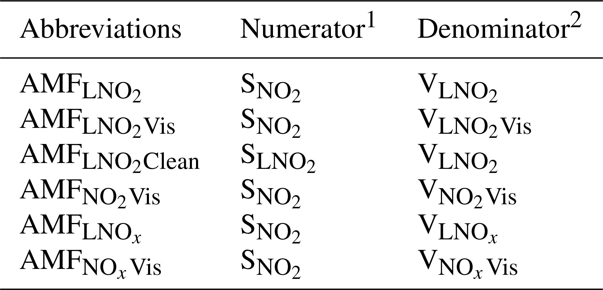
1 The part of simulated VCD seen by OMI. 2 The simulated VCD.
While we used 2400 flashes per box and 8160 strokes per box per 2.4 h time window for detecting LNOx, here we show results obtained when using one flash per box and 3.4 strokes per box in the same time window. We note that the WRF total lightning threshold is also reduced to one flash per box, but we keep the ratio condition unchanged. Briefly, the condition is CRF90_ENTLN1(3.4)_TL1_ratio50 as shown in Table 1.
Similarly, the order of estimated daily PEs is LNO2Clean > LNO2 > NO2Vis > LNO2Vis (Fig. B1). Compared with Fig. 4, the LNO2 per flash and LNOx per flash are larger while PEs based on stroke data are smaller. Considering the additional boxes of fewer lightning counts, differences in the daily mean flashes and NOx result in different PEs, and the relationship presents more like the power function as mentioned in Bucsela et al. (2019).
Instead of using the nonlinear regression of power function
where x is flashes or strokes and y is NO2 or NOx, we take the logarithm of both sides and apply the linear regression to data:
As expected, the linear regression based on logarithmized data performs better in this situation and yields α=38 kmol and β=0.3 for LNOx per flash (Fig. B2). Since we use the unbinned data (flashes not divided into many groups), we compare our results with Bucsela et al. (2019) based on the same kind of data (α=10.3 kmol and β=0.42). The large difference of α is related to the method of estimating LNOx, different lightning data (WWLLN and ENTLN), and different regions (northern midlatitudes and CONUS). Note that the resolution (13 km × 24 km) of OMI could weaken the signal of LNOx. We believe the phenomenon of higher production efficiency as flash rate decreases (Fig. B3) could be explored in much more detail with higher-resolution data like the TROPOMI data.
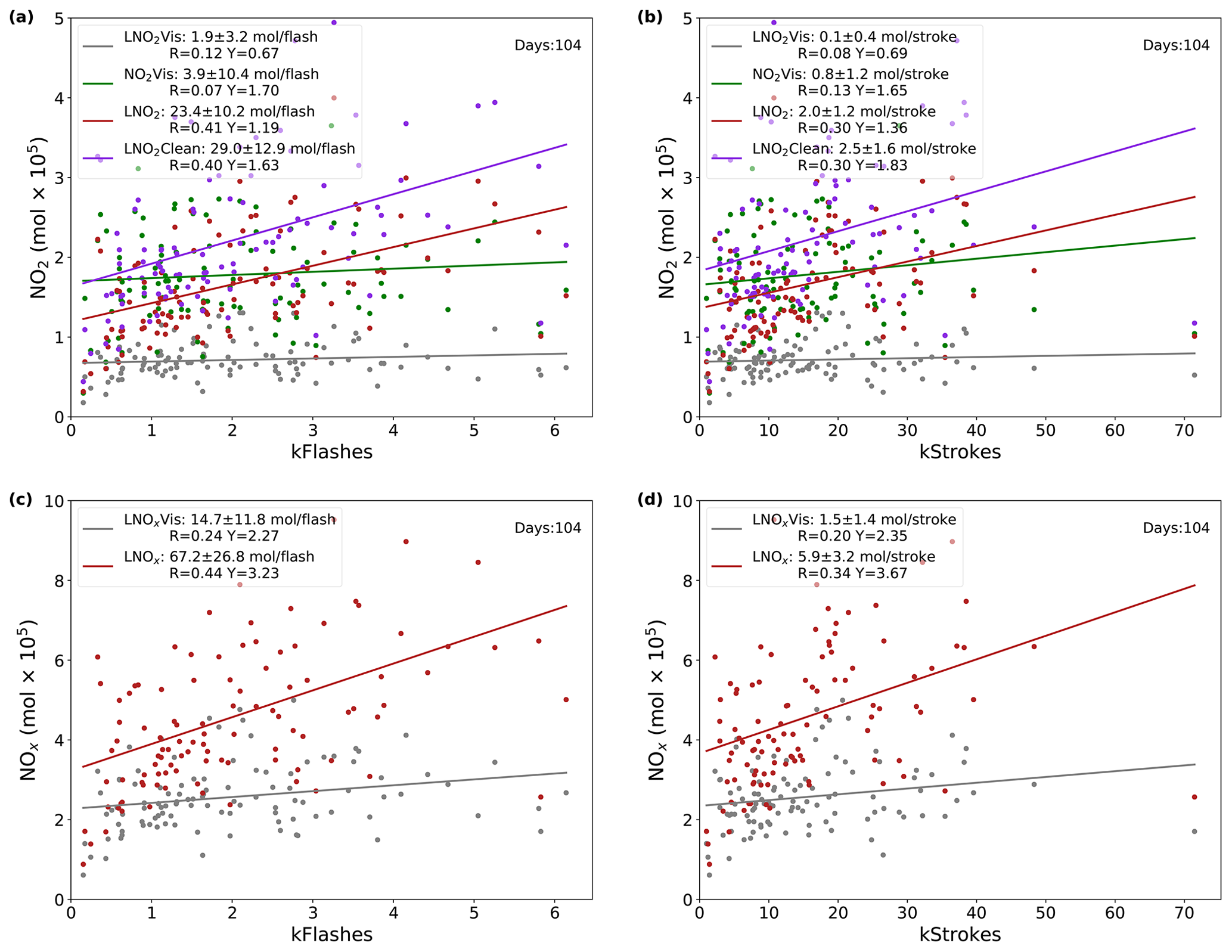
Figure B1Linear regressions with CRF ≥90 % and a flash threshold of one flash per box or 3.4 strokes per box per 2.4 h. (a) Daily NO2Vis, LNO2Vis, LNO2, and LNO2Clean versus ENTLN total flash data. (b) Same as (a) but for strokes. (c) Daily LNOxVis and LNOx versus total flashes. (d) Same as (c) but for strokes.
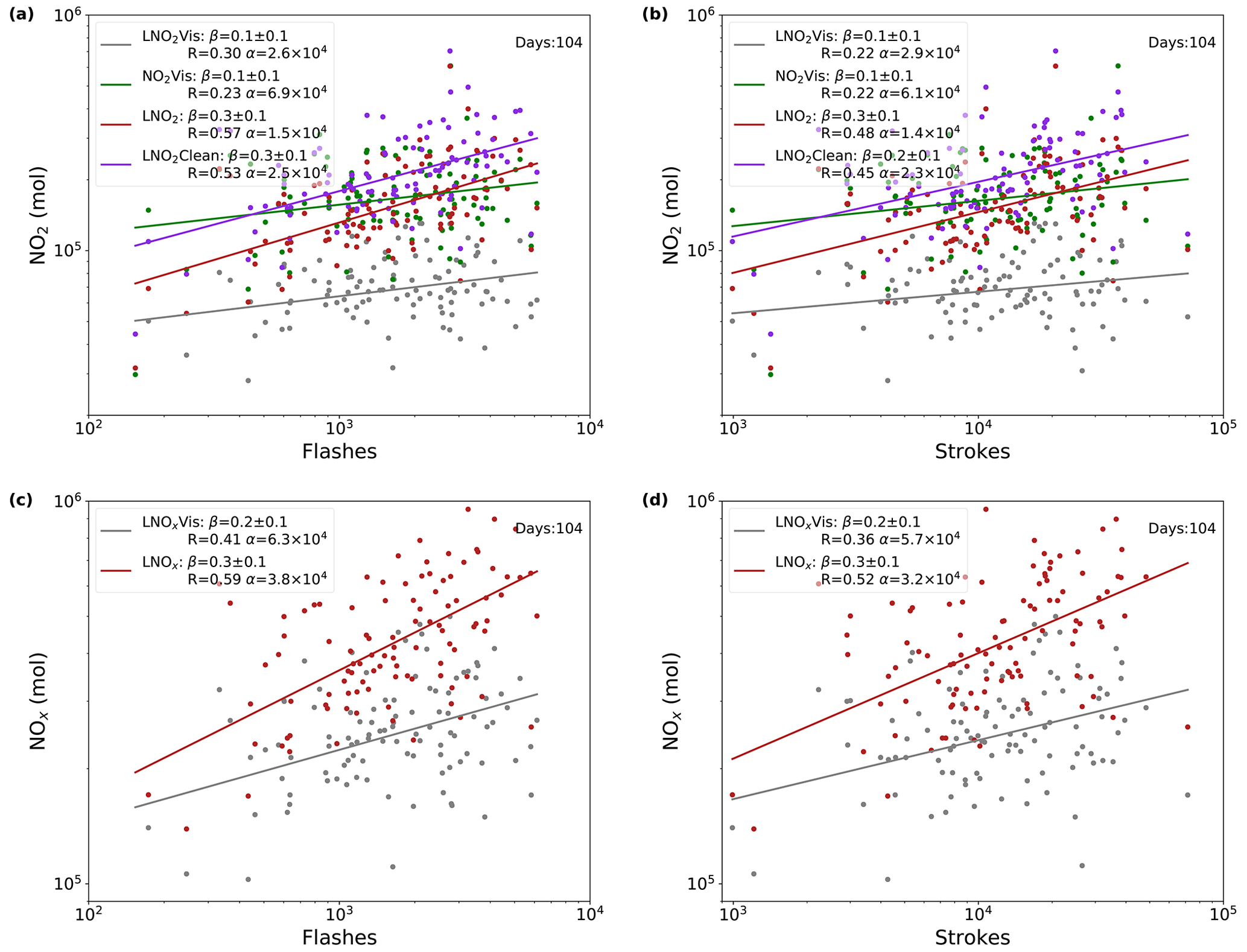
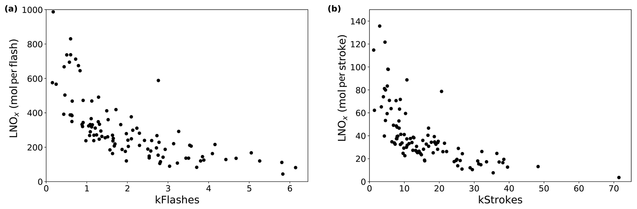
Figure B3(a) Daily LNOx production efficiencies versus ENTLN total flash data, with CRF ≥90 % and a flash threshold of one flash per box. (b) Same as (a) but for strokes.
The retrieval algorithm used in Sect. 2.4 is available at https://github.com/zxdawn/BEHR-LNOx (last access: 20 March 2020; https://doi.org/10.5281/zenodo.3553426, Zhang and Laughner, 2019). The WRF-Chem model output and LNOx product are available upon request to Xin Zhang (xinzhang1215@gmail.com). MOZART-4 global model output is available at https://www.acom.ucar.edu/wrf-chem/mozart.shtml (last access: 20 March 2020).
YY directed the research and RvdA, XZ, and YY designed the research with feedback from the other co-authors; RvdA and XZ developed the algorithm; JLL provided guidance and supporting data on the ENTLN data; XZ performed simulations and analysis with the help of YY, RvdA, QC, XK, SY, JC, CH, and RS; YY, RvdA, JLL, and XZ interpreted the data and discussed the results. XZ drafted the manuscript with comments from the co-authors; JLL, RvdA, and YY edited the manuscript.
The authors declare that they have no conflict of interest.
We acknowledge use of the computational resources provided by the National Supercomputer Centre in Guangzhou (NSCC-GZ). We thank the University of California Berkeley Satellite Group for the basic BEHR algorithm. We also thank Earth Networks Company for providing the Earth Networks Total Lightning Network (ENTLN) datasets. We appreciate the discussions with Joshua L. Laughner for BEHR codes and Mary Barth for the WRF-Chem lightning NOx module. The authors would also like to thank all anonymous reviewers as well as Kenneth E. Pickering, Eric J. Bucsela, and Dale J. Allen for detailed comments which greatly improved this paper. Finally, we thank all contributors of Python packages used in this paper (Met Office, 2010–2015; Hoyer and Hamman, 2017; Hunter, 2007; Zhuang et al., 2019; McKinney, 2011; Inc., 2015; Seabold and Perktold, 2010; van der Walt et al., 2011; Waskom et al., 2017).
This research has been supported by the National Natural Science Foundation of China (grant nos. 91644224 and 41705118).
This paper was edited by Steffen Beirle and reviewed by three anonymous referees.
Acarreta, J. R., de Haan, J. F., and Stammes, P.: Cloud pressure retrieval using the O2-O2 absorption band at 477 nm, J. Geophys. Res., 109, 2165, https://doi.org/10.1029/2003JD003915, 2004. a, b, c
Allen, D. J., Pickering, K. E., Duncan, B. N., and Damon, M.: Impact of lightning NO emissions on North American photochemistry as determined using the Global Modeling Initiative (GMI) model, J. Geophys. Res., 115, 4711, https://doi.org/10.1029/2010JD014062, 2010. a
Allen, D. J., Pickering, K. E., Pinder, R. W., Henderson, B. H., Appel, K. W., and Prados, A.: Impact of lightning-NO on eastern United States photochemistry during the summer of 2006 as determined using the CMAQ model, Atmos. Chem. Phys., 12, 1737–1758, https://doi.org/10.5194/acp-12-1737-2012, 2012. a
Allen, D. J., Pickering, K. E., Bucsela, E. J., Krotkov, N., and Holzworth, R.: Lightning NOx Production in the Tropics as Determined Using OMI NO2 Retrievals and WWLLN Stroke Data, J. Geophys. Res.-Atmos., 124, 13498–13518, https://doi.org/10.1029/2018JD029824, 2019. a, b, c, d, e
Banerjee, A., Archibald, A. T., Maycock, A. C., Telford, P., Abraham, N. L., Yang, X., Braesicke, P., and Pyle, J. A.: Lightning NOx, a key chemistry–climate interaction: impacts of future climate change and consequences for tropospheric oxidising capacity, Atmos. Chem. Phys., 14, 9871–9881, https://doi.org/10.5194/acp-14-9871-2014, 2014. a
Barth, M. C., Lee, J., Hodzic, A., Pfister, G., Skamarock, W. C., Worden, J., Wong, J., and Noone, D.: Thunderstorms and upper troposphere chemistry during the early stages of the 2006 North American Monsoon, Atmos. Chem. Phys., 12, 11003–11026, https://doi.org/10.5194/acp-12-11003-2012, 2012. a, b
Beirle, S., Platt, U., Wenig, M., and Wagner, T.: NOx production by lightning estimated with GOME, Adv. Space Res., 34, 793–797, https://doi.org/10.1016/j.asr.2003.07.069, 2004. a
Beirle, S., Spichtinger, N., Stohl, A., Cummins, K. L., Turner, T., Boccippio, D., Cooper, O. R., Wenig, M., Grzegorski, M., Platt, U., and Wagner, T.: Estimating the NOx produced by lightning from GOME and NLDN data: a case study in the Gulf of Mexico, Atmos. Chem. Phys., 6, 1075–1089, https://doi.org/10.5194/acp-6-1075-2006, 2006. a
Beirle, S., Salzmann, M., Lawrence, M. G., and Wagner, T.: Sensitivity of satellite observations for freshly produced lightning NOx, Atmos. Chem. Phys., 9, 1077–1094, https://doi.org/10.5194/acp-9-1077-2009, 2009. a, b
Beirle, S., Huntrieser, H., and Wagner, T.: Direct satellite observation of lightning-produced NOx, Atmos. Chem. Phys., 10, 10965–10986, https://doi.org/10.5194/acp-10-10965-2010, 2010. a, b, c
Bela, M. M., Barth, M. C., Toon, O. B., Fried, A., Homeyer, C. R., Morrison, H., Cummings, K. A., Li, Y., Pickering, K. E., Allen, D. J., Yang, Q., Wennberg, P. O., Crounse, J. D., St. Clair, J. M., Teng, A. P., O'Sullivan, D., Huey, L. G., Chen, D., Liu, X., Blake, D. R., Blake, N. J., Apel, E. C., Hornbrook, R. S., Flocke, F., Campos, T., and Diskin, G.: Wet scavenging of soluble gases in DC3 deep convective storms using WRF-Chem simulations and aircraft observations, J. Geophys. Res.-Atmos., 121, 4233–4257, https://doi.org/10.1002/2015JD024623, 2016. a
Boersma, K. F., Eskes, H. J., Meijer, E. W., and Kelder, H. M.: Estimates of lightning NOx production from GOME satellite observations, Atmos. Chem. Phys., 5, 2311–2331, https://doi.org/10.5194/acp-5-2311-2005, 2005. a
Boersma, K. F., Eskes, H. J., Richter, A., De Smedt, I., Lorente, A., Beirle, S., van Geffen, J. H. G. M., Zara, M., Peters, E., Van Roozendael, M., Wagner, T., Maasakkers, J. D., van der A, R. J., Nightingale, J., De Rudder, A., Irie, H., Pinardi, G., Lambert, J.-C., and Compernolle, S. C.: Improving algorithms and uncertainty estimates for satellite NO2 retrievals: results from the quality assurance for the essential climate variables (QA4ECV) project, Atmos. Meas. Tech., 11, 6651–6678, https://doi.org/10.5194/amt-11-6651-2018, 2018. a
Bovensmann, H., Burrows, J. P., Buchwitz, M., Frerick, J., Noël, S., Rozanov, V. V., Chance, K. V., and Goede, A. P. H.: SCIAMACHY: Mission Objectives and Measurement Modes, J. Atmos. Sci., 56, 127–150, https://doi.org/10.1175/1520-0469(1999)056<0127:SMOAMM>2.0.CO;2, 1999. a
Browne, E. C., Wooldridge, P. J., Min, K.-E., and Cohen, R. C.: On the role of monoterpene chemistry in the remote continental boundary layer, Atmos. Chem. Phys., 14, 1225–1238, https://doi.org/10.5194/acp-14-1225-2014, 2014. a
Bucsela, E. J., Pickering, K. E., Huntemann, T. L., Cohen, R. C., Perring, A., Gleason, J. F., Blakeslee, R. J., Albrecht, R. I., Holzworth, R., Cipriani, J. P., Vargas-Navarro, D., Mora-Segura, I., Pacheco-Hernández, A., and Laporte-Molina, S.: Lightning-generated NOx seen by the Ozone Monitoring Instrument during NASA's Tropical Composition, Cloud and Climate Coupling Experiment (TC4), J. Geophys. Res., 115, 793, https://doi.org/10.1029/2009JD013118, 2010. a, b, c, d, e
Bucsela, E. J., Krotkov, N. A., Celarier, E. A., Lamsal, L. N., Swartz, W. H., Bhartia, P. K., Boersma, K. F., Veefkind, J. P., Gleason, J. F., and Pickering, K. E.: A new stratospheric and tropospheric NO2 retrieval algorithm for nadir-viewing satellite instruments: applications to OMI, Atmos. Meas. Tech., 6, 2607–2626, https://doi.org/10.5194/amt-6-2607-2013, 2013. a, b, c, d
Bucsela, E. J., Pickering, K. E., Allen, D. J., Holzworth, R., and Krotkov, N. A.: Midlatitude lightning NOx production efficiency inferred from OMI and WWLLN data, J. Geophys. Res.-Atmos., 124, 13475–13497, https://doi.org/10.1029/2019JD030561, 2019. a, b, c, d, e, f, g, h, i, j, k
Burrows, J. P., Weber, M., Buchwitz, M., Rozanov, V., Ladstätter-Weißenmayer, A., Richter, A., DeBeek, R., Hoogen, R., Bramstedt, K., Eichmann, K.-U., Eisinger, M., and Perner, D.: The Global Ozone Monitoring Experiment (GOME): Mission Concept and First Scientific Results, J. Atmos. Sci., 56, 151–175, https://doi.org/10.1175/1520-0469(1999)056<0151:TGOMEG>2.0.CO;2, 1999. a
Callies, J., Corpaccioli, E., Eisinger, M., Hahne, A., and Lefebvre, A.: GOME-2-Metop's second-generation sensor for operational ozone monitoring, ESA Bulletin, 102, 28–36, 2000. a
Carey, L. D., Koshak, W., Peterson, H., and Mecikalski, R. M.: The kinematic and microphysical control of lightning rate, extent, and NOx production, J. Geophys. Res.-Atmos., 121, 7975–7989, https://doi.org/10.1002/2015JD024703, 2016. a
Choi, S., Joiner, J., Choi, Y., Duncan, B. N., Vasilkov, A., Krotkov, N., and Bucsela, E.: First estimates of global free-tropospheric NO2 abundances derived using a cloud-slicing technique applied to satellite observations from the Aura Ozone Monitoring Instrument (OMI), Atmos. Chem. Phys., 14, 10565–10588, https://doi.org/10.5194/acp-14-10565-2014, 2014. a, b
Clark, S. K., Ward, D. S., and Mahowald, N. M.: Parameterization-based uncertainty in future lightning flash density, Geophys. Res. Lett., 44, 2893–2901, https://doi.org/10.1002/2017GL073017, 2017. a
Davis, T. C., Rutledge, S. A., and Fuchs, B. R.: Lightning location, NOx production, and transport by anomalous and normal polarity thunderstorms, J. Geophys. Res.-Atmos., 124, 8722–8742, https://doi.org/10.1029/2018JD029979, 2019. a
DeCaria, A. J., Pickering, K. E., Stenchikov, G. L., Scala, J. R., Stith, J. L., Dye, J. E., Ridley, B. A., and Laroche, P.: A cloud-scale model study of lightning-generated NOx in an individual thunderstorm during STERAO-A, J. Geophys. Res., 105, 11601–11616, https://doi.org/10.1029/2000JD900033, 2000. a
DeCaria, A. J., Pickering, K. E., Stenchikov, G. L., and Ott, L. E.: Lightning-generated NOx and its impact on tropospheric ozone production: A three-dimensional modeling study of a Stratosphere-Troposphere Experiment: Radiation, Aerosols and Ozone (STERAO-A) thunderstorm, J. Geophys. Res., 110, D14303, https://doi.org/10.1029/2004JD005556, 2005. a, b
Dobber, M., Kleipool, Q., Dirksen, R., Levelt, P., Jaross, G., Taylor, S., Kelly, T., Flynn, L., Leppelmeier, G., and Rozemeijer, N.: Validation of Ozone Monitoring Instrument level 1b data products, J. Geophys. Res., 113, 5224, https://doi.org/10.1029/2007JD008665, 2008. a, b
Emmons, L. K., Walters, S., Hess, P. G., Lamarque, J.-F., Pfister, G. G., Fillmore, D., Granier, C., Guenther, A., Kinnison, D., Laepple, T., Orlando, J., Tie, X., Tyndall, G., Wiedinmyer, C., Baughcum, S. L., and Kloster, S.: Description and evaluation of the Model for Ozone and Related chemical Tracers, version 4 (MOZART-4), Geosci. Model Dev., 3, 43–67, https://doi.org/10.5194/gmd-3-43-2010, 2010. a
EPA: 2011 National Emissions Inventory, version 2–Technical support document, US Environmental Protection Agency, Office of Air Quality Planning and Standards, available at: https://www.epa.gov/air-emissions-inventories/2011-national-emissions-inventory-nei-technical-support-document (last access: 3 April 2020), 2015. a
EPA and OAR: Air Pollutant Emissions Trends Data | US EPA, available at: https://www.epa.gov/air-emissions-inventories/air-pollutant-emissions-trends-data (last access: 3 April 2020), 2015. a
Finney, D. L., Doherty, R. M., Wild, O., Young, P. J., and Butler, A.: Response of lightning NOx emissions and ozone production to climate change: Insights from the Atmospheric Chemistry and Climate Model Intercomparison Project, Geophys. Res. Lett., 43, 5492–5500, https://doi.org/10.1002/2016GL068825, 2016. a
Finney, D. L., Doherty, R. M., Wild, O., Stevenson, D. S., MacKenzie, I. A., and Blyth, A. M.: A projected decrease in lightning under climate change, Nat. Clim. Change, 8, 210–213, https://doi.org/10.1038/s41558-018-0072-6, 2018. a, b, c
Fried, A., Barth, M. C., Bela, M., Weibring, P., Richter, D., Walega, J., Li, Y., Pickering, K., Apel, E., Hornbrook, R., Hills, A., Riemer, D. D., Blake, N., Blake, D. R., Schroeder, J. R., Luo, Z. J., Crawford, J. H., Olson, J., Rutledge, S., Betten, D., Biggerstaff, M. I., Diskin, G. S., Sachse, G., Campos, T., Flocke, F., Weinheimer, A., Cantrell, C., Pollack, I., Peischl, J., Froyd, K., Wisthaler, A., Mikoviny, T., and Woods, S.: Convective transport of formaldehyde to the upper troposphere and lower stratosphere and associated scavenging in thunderstorms over the central United States during the 2012 DC3 study, J. Geophys. Res.-Atmos., 121, 7430–7460, https://doi.org/10.1002/2015JD024477, 2016. a
Fuchs, B. R. and Rutledge, S. A.: Investigation of Lightning Flash Locations in Isolated Convection Using LMA Observations, J. Geophys. Res.-Atmos., 123, 6158–6174, https://doi.org/10.1002/2017JD027569, 2018. a
Goliff, W. S., Stockwell, W. R., and Lawson, C. V.: The regional atmospheric chemistry mechanism, version 2, Atmos. Environ., 68, 174–185, https://doi.org/10.1016/j.atmosenv.2012.11.038, 2013. a
Grell, G. A., Peckham, S. E., Schmitz, R., McKeen, S. A., Frost, G., Skamarock, W. C., and Eder, B.: Fully coupled “online” chemistry within the WRF model, Atmos. Environ., 39, 6957–6975, https://doi.org/10.1016/j.atmosenv.2005.04.027, 2005. a
Griffin, D., Zhao, X., McLinden, C. A., Boersma, F., Bourassa, A., Dammers, E., Degenstein, D., Eskes, H., Fehr, L., Fioletov, V., Hayden, K., Kharol, S. K., Li, S.-M., Makar, P., Martin, R. V., Mihele, C., Mittermeier, R. L., Krotkov, N., Sneep, M., Lamsal, L. N., Linden, M. T., van Geffen, J., Veefkind, P., and Wolde, M.: High-Resolution Mapping of Nitrogen Dioxide With TROPOMI: First Results and Validation Over the Canadian Oil Sands, Geophys. Res. Lett., 46, 1049–1060, https://doi.org/10.1029/2018GL081095, 2019. a
Guenther, A., Karl, T., Harley, P., Wiedinmyer, C., Palmer, P. I., and Geron, C.: Estimates of global terrestrial isoprene emissions using MEGAN (Model of Emissions of Gases and Aerosols from Nature), Atmos. Chem. Phys., 6, 3181–3210, https://doi.org/10.5194/acp-6-3181-2006, 2006. a
Hauglustaine, D., Emmons, L., Newchurch, M., Brasseur, G., Takao, T., Matsubara, K., Johnson, J., Ridley, B., Stith, J., and Dye, J.: On the Role of Lightning NOx in the Formation of Tropospheric Ozone Plumes: A Global Model Perspective, J. Atmos. Chem., 38, 277–294, https://doi.org/10.1023/A:1006452309388, 2001. a
Hoyer, S. and Hamman, J.: xarray: N-D labeled arrays and datasets in Python, Journal of Open Research Software, 5, 10, https://doi.org/10.5334/jors.148, 2017. a
Hunter, J. D.: Matplotlib: A 2D Graphics Environment, Comput. Sci. Eng., 9, 90–95, https://doi.org/10.1109/MCSE.2007.55, 2007. a
Inc.: Collaborative data science, available at: https://plot.ly (last access: 3 April 2020), 2015. a
Joiner, J., Vasilkov, A. P., Gupta, P., Bhartia, P. K., Veefkind, P., Sneep, M., de Haan, J., Polonsky, I., and Spurr, R.: Fast simulators for satellite cloud optical centroid pressure retrievals; evaluation of OMI cloud retrievals, Atmos. Meas. Tech., 5, 529–545, https://doi.org/10.5194/amt-5-529-2012, 2012. a
KNMI: Background information about the Row Anomaly in OMI, available at: http://projects.knmi.nl/omi/research/product/rowanomaly-background.php, (last access: 3 April 2020), 2012. a
Krause, A., Kloster, S., Wilkenskjeld, S., and Paeth, H.: The sensitivity of global wildfires to simulated past, present, and future lightning frequency, J. Geophys. Res.-Biogeo., 119, 312–322, https://doi.org/10.1002/2013JG002502, 2014. a
Krotkov, N. A., Lamsal, L. N., Celarier, E. A., Swartz, W. H., Marchenko, S. V., Bucsela, E. J., Chan, K. L., Wenig, M., and Zara, M.: The version 3 OMI NO2 standard product, Atmos. Meas. Tech., 10, 3133–3149, https://doi.org/10.5194/amt-10-3133-2017, 2017. a, b, c
Kuhlmann, G., Hartl, A., Cheung, H. M., Lam, Y. F., and Wenig, M. O.: A novel gridding algorithm to create regional trace gas maps from satellite observations, Atmos. Meas. Tech., 7, 451–467, https://doi.org/10.5194/amt-7-451-2014, 2014. a
Lapierre, J. L., Laughner, J. L., Geddes, J. A., Koshak, W., Cohen, R. C., and Pusede, S. E.: Observing U.S. regional variability in lightning NO2 production rates, J. Geophys. Res.-Atmos., 125, e2019JD031362, https://doi.org/10.1029/2019JD031362, 2020. a, b, c, d, e, f, g, h, i, j, k, l, m, n, o, p, q, r, s, t, u, v, w
Laughner, J. L. and Cohen, R. C.: Quantification of the effect of modeled lightning NO2 on UV–visible air mass factors, Atmos. Meas. Tech., 10, 4403–4419, https://doi.org/10.5194/amt-10-4403-2017, 2017. a, b, c, d
Laughner, J. L., Zhu, Q., and Cohen, R. C.: The Berkeley High Resolution Tropospheric NO2 product, Earth Syst. Sci. Data, 10, 2069–2095, https://doi.org/10.5194/essd-10-2069-2018, 2018. a, b
Laughner, J. L., Zhu, Q., and Cohen, R. C.: Evaluation of version 3.0B of the BEHR OMI NO2 product, Atmos. Meas. Tech., 12, 129–146, https://doi.org/10.5194/amt-12-129-2019, 2019. a, b, c, d, e, f, g
Levelt, P. F., van den Oord, G., Dobber, M. R., Malkki, A., Visser, H., Vries, J. D., Stammes, P., Lundell, J., and Saari, H.: The ozone monitoring instrument, IEEE T. Geosci. Remote, 44, 1093–1101, https://doi.org/10.1109/TGRS.2006.872333, 2006. a, b
Levelt, P. F., Joiner, J., Tamminen, J., Veefkind, J. P., Bhartia, P. K., Stein Zweers, D. C., Duncan, B. N., Streets, D. G., Eskes, H., van der A, R., McLinden, C., Fioletov, V., Carn, S., de Laat, J., DeLand, M., Marchenko, S., McPeters, R., Ziemke, J., Fu, D., Liu, X., Pickering, K., Apituley, A., González Abad, G., Arola, A., Boersma, F., Chan Miller, C., Chance, K., de Graaf, M., Hakkarainen, J., Hassinen, S., Ialongo, I., Kleipool, Q., Krotkov, N., Li, C., Lamsal, L., Newman, P., Nowlan, C., Suleiman, R., Tilstra, L. G., Torres, O., Wang, H., and Wargan, K.: The Ozone Monitoring Instrument: overview of 14 years in space, Atmos. Chem. Phys., 18, 5699–5745, https://doi.org/10.5194/acp-18-5699-2018, 2018. a
Li, Y., Pickering, K. E., Allen, D. J., Barth, M. C., Bela, M. M., Cummings, K. A., Carey, L. D., Mecikalski, R. M., Fierro, A. O., Campos, T. L., Weinheimer, A. J., Diskin, G. S., and Biggerstaff, M. I.: Evaluation of deep convective transport in storms from different convective regimes during the DC3 field campaign using WRF-Chem with lightning data assimilation, J. Geophys. Res.-Atmos., 122, 7140–7163, https://doi.org/10.1002/2017JD026461, 2017. a
Li, Y., Pickering, K. E., Barth, M. C., Bela, M. M., Cummings, K. A., and Allen, D. J.: Evaluation of Parameterized Convective Transport of Trace Gases in Simulation of Storms Observed During the DC3 Field Campaign, J. Geophys. Res.-Atmos., 123, 11238–11261, https://doi.org/10.1029/2018JD028779, 2018. a
Luo, C., Wang, Y., and Koshak, W. J.: Development of a self-consistent lightning NOx simulation in large-scale 3-D models, J. Geophys. Res.-Atmos., 122, 3141–3154, https://doi.org/10.1002/2016JD026225, 2017. a
Marais, E. A., Jacob, D. J., Choi, S., Joiner, J., Belmonte-Rivas, M., Cohen, R. C., Beirle, S., Murray, L. T., Schiferl, L. D., Shah, V., and Jaeglé, L.: Nitrogen oxides in the global upper troposphere: interpreting cloud-sliced NO2 observations from the OMI satellite instrument, Atmos. Chem. Phys., 18, 17017–17027, https://doi.org/10.5194/acp-18-17017-2018, 2018. a
Martin, R. V., Sauvage, B., Folkins, I., Sioris, C. E., Boone, C., Bernath, P., and Ziemke, J.: Space-based constraints on the production of nitric oxide by lightning, J. Geophys. Res., 112, 1479, https://doi.org/10.1029/2006JD007831, 2007. a
McKinney, W.: pandas: a foundational Python library for data analysis and statistics, Python for High Performance and Scientific Computing, 14, 2011. a
Mecikalski, R. M. and Carey, L. D.: Lightning characteristics relative to radar, altitude and temperature for a multicell, MCS and supercell over northern Alabama, Atmos. Res., 191, 128–140, https://doi.org/10.1016/j.atmosres.2017.03.001, 2017. a
Met Office: Cartopy: a cartographic python library with a matplotlib interface, Exeter, Devon, available at: http://scitools.org.uk/cartopy (last access: 3 April 2020), 2010–2015. a
Min, M., Wu, C., Li, C., Liu, H., Xu, N., Wu, X., Chen, L., Wang, F., Sun, F., Qin, D., Wang, X., Li, B., Zheng, Z., Cao, G., and Dong, L.: Developing the science product algorithm testbed for Chinese next-generation geostationary meteorological satellites: Fengyun-4 series, J. Meteorol. Res., 31, 708–719, https://doi.org/10.1007/s13351-017-6161-z, 2017. a
Myhre, G., Shindell, D., Bréon, F. M., Collins, W., Fuglestvedt, J., Huang, J., Koch, D., Lamarque, J. F., Lee, D., and Mendoza, B.: Climate change 2013: the physical science basis. Contribution of Working Group I to the Fifth Assessment Report of the Intergovernmental Panel on Climate Change, edited by: Tignor, M., Allen, S. K., Boschung, J., Nauels, A., Xia, Y., Bex, V., and Midgley, P. M., Cambridge University Press Cambridge, UK and New York, NY, USA, 2013. a
Nault, B. A., Garland, C., Wooldridge, P. J., Brune, W. H., Campuzano-Jost, P., Crounse, J. D., Day, D. A., Dibb, J., Hall, S. R., Huey, L. G., Jimenez, J. L., Liu, X., Mao, J., Mikoviny, T., Peischl, J., Pollack, I. B., Ren, X., Ryerson, T. B., Scheuer, E., Ullmann, K., Wennberg, P. O., Wisthaler, A., Zhang, L., and Cohen, R. C.: Observational Constraints on the Oxidation of NO x in the Upper Troposphere, J. Phys. Chem. A, 120, 1468–1478, https://doi.org/10.1021/acs.jpca.5b07824, 2016. a
Nault, B. A., Laughner, J. L., Wooldridge, P. J., Crounse, J. D., Dibb, J., Diskin, G., Peischl, J., Podolske, J. R., Pollack, I. B., Ryerson, T. B., Scheuer, E., Wennberg, P. O., and Cohen, R. C.: Lightning NOx Emissions: Reconciling Measured and Modeled Estimates With Updated NOx Chemistry, Geophys. Res. Lett., 44, 9479–9488, https://doi.org/10.1002/2017GL074436, 2017. a, b, c, d
Ott, L. E., Pickering, K. E., Stenchikov, G. L., Huntrieser, H., and Schumann, U.: Effects of lightning NO x production during the 21 July European Lightning Nitrogen Oxides Project storm studied with a three-dimensional cloud-scale chemical transport model, J. Geophys. Res., 112, D05307, https://doi.org/10.1029/2006JD007365, 2007. a
Ott, L. E., Pickering, K. E., Stenchikov, G. L., Allen, D. J., DeCaria, A. J., Ridley, B., Lin, R.-F., Lang, S., and Tao, W.-K.: Production of lightning NOx and its vertical distribution calculated from three-dimensional cloud-scale chemical transport model simulations, J. Geophys. Res., 115, 4711, https://doi.org/10.1029/2009JD011880, 2010. a, b
Pickering, K. E., Thompson, A. M., Wang, Y., Tao, W.-K., McNamara, D. P., Kirchhoff, V. W. J. H., Heikes, B. G., Sachse, G. W., Bradshaw, J. D., Gregory, G. L., and Blake, D. R.: Convective transport of biomass burning emissions over Brazil during TRACE A, J. Geophys. Res., 101, 23993–24012, https://doi.org/10.1029/96JD00346, 1996. a
Pickering, K. E., Bucsela, E., Allen, D., Ring, A., Holzworth, R., and Krotkov, N.: Estimates of lightning NOx production based on OMI NO2 observations over the Gulf of Mexico, J. Geophys. Res.-Atmos., 121, 8668–8691, https://doi.org/10.1002/2015JD024179, 2016. a, b, c, d, e, f, g, h, i, j, k, l, m, n, o, p, q, r, s, t, u
Platt, U. and Perner, D.: Measurements of Atmospheric Trace Gases by Long Path Differential UV/Visible Absorption Spectroscopy, in: Optical and Laser Remote Sensing, edited by: Schawlow, A. L., Killinger, D. K., and Mooradian, A., vol. 39 of Springer Series in Optical Sciences, 97–105, Springer Berlin Heidelberg, Berlin, Heidelberg, https://doi.org/10.1007/978-3-540-39552-2_13, 1983. a
Price, C. and Rind, D.: A simple lightning parameterization for calculating global lightning distributions, J. Geophys. Res., 97, 9919–9933, https://doi.org/10.1029/92JD00719, 1992. a
Richter, A., Burrows, J. P., Nüß, H., Granier, C., and Niemeier, U.: Increase in tropospheric nitrogen dioxide over China observed from space, Nature, 437, 129–132, https://doi.org/10.1038/nature04092, 2005. a
Romps, D. M.: Evaluating the future of lightning in cloud-resolving models, 46, 14863–14871, Geophys. Res. Lett., https://doi.org/10.1029/2019GL085748, 2019. a
Romps, D. M., Seeley, J. T., Vollaro, and Molinari, J.: Projected increase in lightning strikes in the United States due to global warming, Science, 346, 851–854, https://doi.org/10.1126/science.1259100, 2014. a
Rudlosky, S.: Evaluating ENTLN performance relative to TRMM/LIS, Journal of Operational Meteorology, 3, 11–20, https://doi.org/10.15191/nwajom.2015.0302, 2015. a
Schaaf, C. B., Liu, J., Gao, F., and Strahler, A. H.: Aqua and Terra MODIS Albedo and Reflectance Anisotropy Products, in: Land Remote Sensing and Global Environmental Change, edited by: Ramachandran, B., Justice, C. O., and Abrams, M. J., vol. 11 of Remote Sensing and Digital Image Processing, 549–561, Springer New York, New York, NY, https://doi.org/10.1007/978-1-4419-6749-7_24, 2011. a
Schumann, U. and Huntrieser, H.: The global lightning-induced nitrogen oxides source, Atmos. Chem. Phys., 7, 3823–3907, https://doi.org/10.5194/acp-7-3823-2007, 2007. a, b
Schwantes, R. H., Teng, A. P., Nguyen, T. B., Coggon, M. M., Crounse, J. D., St Clair, J. M., Zhang, X., Schilling, K. A., Seinfeld, J. H., and Wennberg, P. O.: Isoprene NO3 Oxidation Products from the RO2+HO2 Pathway, J. Phys. Chem. A, 119, 10158–10171, https://doi.org/10.1021/acs.jpca.5b06355, 2015. a
Seabold, S. and Perktold, J.: statsmodels: Econometric and statistical modeling with python, in: 9th Python in Science Conference, 28 June–3 July, Austin, Texas, available at: https://conference.scipy.org/proceedings/scipy2010/seabold.html (last access: 3 April 2020), 2010. a
Silvern, R. F., Jacob, D. J., Travis, K. R., Sherwen, T., Evans, M. J., Cohen, R. C., Laughner, J. L., Hall, S. R., Ullmann, K., Crounse, J. D., Wennberg, P. O., Peischl, J., and Pollack, I. B.: Observed NO∕NO2 ratios in the upper troposphere imply errors in cycling kinetics or an unaccounted NOx reservoir, Geophys. Res. Lett., 45, 4466–4474, https://doi.org/10.1029/2018GL077728, 2018. a, b
Sneep, M., de Haan, J. F., Stammes, P., Wang, P., Vanbauce, C., Joiner, J., Vasilkov, A. P., and Levelt, P. F.: Three-way comparison between OMI and PARASOL cloud pressure products, J. Geophys. Res., 113, D05204, https://doi.org/10.1029/2007JD008694, 2008. a
Stammes, P., Sneep, M., de Haan, J. F., Veefkind, J. P., Wang, P., and Levelt, P. F.: Effective cloud fractions from the Ozone Monitoring Instrument: Theoretical framework and validation, J. Geophys. Res., 113, D05204, https://doi.org/10.1029/2007JD008820, 2008. a
Strode, S. A., Douglass, A. R., Ziemke, J. R., Manyin, M., Nielsen, J. E., and Oman, L. D.: A Model and Satellite-Based Analysis of the Tropospheric Ozone Distribution in Clear Versus Convectively Cloudy Conditions, J. Geophys. Res.-Atmos., 122, 11948–11960, https://doi.org/10.1002/2017JD027015, 2017. a, b, c
Travis, K. R., Jacob, D. J., Fisher, J. A., Kim, P. S., Marais, E. A., Zhu, L., Yu, K., Miller, C. C., Yantosca, R. M., Sulprizio, M. P., Thompson, A. M., Wennberg, P. O., Crounse, J. D., St. Clair, J. M., Cohen, R. C., Laughner, J. L., Dibb, J. E., Hall, S. R., Ullmann, K., Wolfe, G. M., Pollack, I. B., Peischl, J., Neuman, J. A., and Zhou, X.: Why do models overestimate surface ozone in the Southeast United States?, Atmos. Chem. Phys., 16, 13561–13577, https://doi.org/10.5194/acp-16-13561-2016, 2016. a
van der Walt, S., Colbert, S. C., and Varoquaux, G.: The NumPy Array: A Structure for Efficient Numerical Computation, Comput. Sci. Eng., 13, 22–30, https://doi.org/10.1109/MCSE.2011.37, 2011. a
Vasilkov, A., Joiner, J., Spurr, R., Bhartia, P. K., Levelt, P., and Stephens, G.: Evaluation of the OMI cloud pressures derived from rotational Raman scattering by comparisons with other satellite data and radiative transfer simulations, J. Geophys. Res., 113, D05204, https://doi.org/10.1029/2007JD008689, 2008. a
Veefkind, J. P., Aben, I., McMullan, K., Förster, H., de Vries, J., Otter, G., Claas, J., Eskes, H. J., de Haan, J. F., Kleipool, Q., van Weele, M., Hasekamp, O., Hoogeveen, R., Landgraf, J., Snel, R., Tol, P., Ingmann, P., Voors, R., Kruizinga, B., Vink, R., Visser, H., and Levelt, P. F.: TROPOMI on the ESA Sentinel-5 Precursor: A GMES mission for global observations of the atmospheric composition for climate, air quality and ozone layer applications, Remote Sens. Environ., 120, 70–83, https://doi.org/10.1016/j.rse.2011.09.027, 2012. a
Wang, L., Follette-Cook, M. B., Newchurch, M. J., Pickering, K. E., Pour-Biazar, A., Kuang, S., Koshak, W., and Peterson, H.: Evaluation of lightning-induced tropospheric ozone enhancements observed by ozone lidar and simulated by WRF/Chem, Atmos. Environ., 115, 185–191, https://doi.org/10.1016/j.atmosenv.2015.05.054, 2015. a
Waskom, M., Botvinnik, O., O'Kane, D., Hobson, P., Lukauskas, S., Gemperline, D. C., Augspurger, T., Halchenko, Y., Cole, J. B., Warmenhoven, J., de Ruiter, J., Pye, C., Hoyer, S., Vanderplas, J., Villalba, S., Kunter, G., Quintero, E., Bachant, P., Martin, M., Meyer, K., Miles, A., Ram, Y., Yarkoni, T., Williams, M. L., Evans, C., Fitzgerald, C., Brian, Fonnesbeck, C., Lee, A., and Qalieh, A.: Mwaskom/Seaborn: V0.8.1 (September 2017), https://doi.org/10.5281/zenodo.883859, 2017. a
Williams, E. R.: The tripole structure of thunderstorms, J. Geophys. Res., 94, 13151, https://doi.org/10.1029/JD094iD11p13151, 1989. a
Wong, J., Barth, M. C., and Noone, D.: Evaluating a lightning parameterization based on cloud-top height for mesoscale numerical model simulations, Geosci. Model Dev., 6, 429–443, https://doi.org/10.5194/gmd-6-429-2013, 2013. a, b
Xu, K.-M. and Randall, D. A.: A Semiempirical Cloudiness Parameterization for Use in Climate Models, J. Atmos. Sci., 53, 3084–3102, https://doi.org/10.1175/1520-0469(1996)053<3084:ASCPFU>2.0.CO;2, 1996. a
Yang, J., Zhang, Z., Wei, C., Lu, F., and Guo, Q.: Introducing the New Generation of Chinese Geostationary Weather Satellites, Fengyun-4, B. Am. Meteorol. Soc., 98, 1637–1658, https://doi.org/10.1175/BAMS-D-16-0065.1, 2017. a
Zel'dovich, Y. and Raizer, Y.: VIII – Physical and chemical kinetics in hydrodynamic processes, in: Physics of Shock Waves and High-Temperature Hydrodynamic Phenomena, edited by: Hayes, W. D., Probstein, R. F., Zel'dovich, Y., and Raizer, Y., Academic Press, 566–571, https://doi.org/10.1016/B978-0-12-395672-9.50009-6, 1967. a
Zhang, P., Lu, Q., Hu, X., Gu, S., Yang, L., Min, M., Chen, L., Xu, N., Sun, L., Bai, W., Ma, G., and Di Xian: Latest Progress of the Chinese Meteorological Satellite Program and Core Data Processing Technologies, Adv. Atmos. Sci., 36, 1027–1045, https://doi.org/10.1007/s00376-019-8215-x, 2019. a
Zhang, X. and Laughner, J.: zxdawn/BEHR-LNOx: v1.0, Zenodo, https://doi.org/10.5281/zenodo.3553426, 2019. a
Zhao, C., Wang, Y., Choi, Y., and Zeng, T.: Summertime impact of convective transport and lightning NOx production over North America: modeling dependence on meteorological simulations, Atmos. Chem. Phys., 9, 4315–4327, https://doi.org/10.5194/acp-9-4315-2009, 2009. a
Zhou, Y., Brunner, D., Boersma, K. F., Dirksen, R., and Wang, P.: An improved tropospheric NO2 retrieval for OMI observations in the vicinity of mountainous terrain, Atmos. Meas. Tech., 2, 401–416, https://doi.org/10.5194/amt-2-401-2009, 2009. a
Zhu, Q., Laughner, J. L., and Cohen, R. C.: Lightning NO2 simulation over the contiguous US and its effects on satellite NO2 retrievals, Atmos. Chem. Phys., 19, 13067–13078, https://doi.org/10.5194/acp-19-13067-2019, 2019. a
Zhu, Y., Rakov, V. A., Tran, M. D., and Nag, A.: A study of National Lightning Detection Network responses to natural lightning based on ground truth data acquired at LOG with emphasis on cloud discharge activity, J. Geophys. Res.-Atmos., 121, 14651–14660, https://doi.org/10.1002/2016JD025574, 2016. a
Zhu, Y., Rakov, V. A., Tran, M. D., Stock, M. G., Heckman, S., Liu, C., Sloop, C. D., Jordan, D. M., Uman, M. A., Caicedo, J. A., Kotovsky, D. A., Wilkes, R. A., Carvalho, F. L., Ngin, T., Gamerota, W. R., Pilkey, J. T., and Hare, B. M.: Evaluation of ENTLN Performance Characteristics Based on the Ground Truth Natural and Rocket-Triggered Lightning Data Acquired in Florida, J. Geophys. Res.-Atmos., 122, 9858–9866, https://doi.org/10.1002/2017JD027270, 2017. a
Zhuang, J., Jüling, A., and Rasp, S.: JiaweiZhuang/xESMF: v0.2.1, https://doi.org/10.5281/zenodo.1134365, 2019. a
Ziemke, J. R., Joiner, J., Chandra, S., Bhartia, P. K., Vasilkov, A., Haffner, D. P., Yang, K., Schoeberl, M. R., Froidevaux, L., and Levelt, P. F.: Ozone mixing ratios inside tropical deep convective clouds from OMI satellite measurements, Atmos. Chem. Phys., 9, 573–583, https://doi.org/10.5194/acp-9-573-2009, 2009. a, b
Ziemke, J. R., Strode, S. A., Douglass, A. R., Joiner, J., Vasilkov, A., Oman, L. D., Liu, J., Strahan, S. E., Bhartia, P. K., and Haffner, D. P.: A cloud-ozone data product from Aura OMI and MLS satellite measurements, Atmos. Meas. Tech., 10, 4067–4078, https://doi.org/10.5194/amt-10-4067-2017, 2017. a
- Abstract
- Introduction
- Data and methods
- Results
- Uncertainty analysis
- Conclusions
- Appendix A: AMF definitions used in this study
- Appendix B: LNOx production based on lower lightning thresholds
- Code and data availability
- Author contributions
- Competing interests
- Acknowledgements
- Financial support
- Review statement
- References