A new lidar inversion method using a surface reference target applied to the backscattering coefficient and lidar ratio retrievals of a fog-oil plume at short range

In this paper, a new elastic lidar inversion equation is presented. It is based on the backscattering signal from a surface reference target (SRT) rather than that from a volumetric layer of reference (Rayleigh molecular scatterer) as is usually done. The method presented can be used when the optical properties of such a layer are not available, e.g., in the case of airborne elastic lidar measurements or when the lidar–target line is horizontal Also, a new algorithm is described to retrieve the lidar ratio and the backscattering coefficient of an aerosol plume without any a priori assumptions about the plume. In addition, our algorithm allows a determination of the instrumental constant. This algorithm is theoretically tested, viz. by means of simulated lidar profiles and then using real measurements. Good agreement with available data in the literature has been found.

1 Introduction

Atmospheric aerosols are liquid or solid particles dispersed in the air (Glickman and Zenk, 2000) of natural (volcano, biomass burnings, desert, ocean) or anthropogenic origins. They play an important role not only in cloud formation (DeMott et al., 2010), in radiative forcing (Hansen et al., 1997; Haywood and Boucher, 2000) and more generally for research on the climate change but also in the context of air quality and public health (Baltensperger et al., 2008; Finlayson-Pitts and Pitts, 2000; Popovicheva et al., 2019; Zhang et al., 2018). Their size varies from the nanometer to the millimeter scale (Robert, unpublished). However, a large majority of aerosols have a size between 0.01 and 3 µm (Clark and Whitby, 1967) for which scattering is dominant in the optical domain. The Mie theory is often used, at least statistically (i.e., for a large population of random sized aerosols), although aerosols are not always spherical. The optical backscattering and extinction properties of aerosols are mainly related to their shape (Ceolato et al., 2018), size distribution (Vargas-Ubera et al., 2007), concentration and chemical composition, which is based to their nature (dust, maritime or urban). Lidars are active remote sensing instruments suitable for aerosol detection and characterization (Sicard et al., 2002) over kilometric distances during both day and nighttime.

The optical properties of aerosols are obtained by means of inversion methods using the simple scattering lidar equation. In the 1980s, a stable one-component formulation adapted to lidar applications was proposed by Klett (1981). It has then been extended to a two-component formulation, viz. separating molecular and aerosol contributions, by Fernald (1984) and Klett (1985). The elastic lidar equation is an ill-posed problem in the sense of Hadamard (1908) since one searches for extinction and backscattering coefficients with only a single observable. Several assumptions are therefore required in order to invert the lidar equation.

• i.

  A calibration constant is usually determined from a volumetric layer of the upper atmosphere as a reference target (Vande Hey, 2014). This calibration layer can be very high in altitude; it has recently been moved from the around 32 km to around 36–39 km for the CALIPSO spaceborne lidar in order to reduce uncertainties in the inversion procedure (Kar et al., 2018; Getzewich et al., 2018). This volume is considered to be made only of pure molecular constituents whose optical scattering properties are well known (Rayleigh regime). The molecular backscattering coefficient is generally estimated from the standard model of the atmosphere (Anon, 1976; Bodhaine et al., 1999). However, poor estimates of the reference or low signal-to-noise ratios (SNRs) can lead to severe uncertainties in the retrieved extinction and backscattering coefficients. Few sensitivity studies have been performed to evaluate such uncertainties (Matsumoto and Takeuchi, 1994; Rocadenbosch et al., 2012). Spatial averaging around the volume of reference in addition to time averaging is thus recommended to increase SNR.

• ii.

  Lidar ratio is constant over the distance range of measurements (Sasano et al., 1985). This is also an important source of errors in the retrieval values. Some studies have proposed a variable lidar ratio under the form of a power-law relationship between the extinction and backscattering coefficients, but such a method requires a priori knowledge of the medium under study (Klett, 1985).

• iii.

  The molecular contribution along the lidar line is known. It is estimated, as for the backscattering coefficient, by means of temperature and pressure vertical profiles, using either the standard model of the atmosphere or radio soundings (Jäger, 2005).

In the case of elastic lidar inversion, the most critical parameter is the lidar ratio (LR). It depends on the wavelength (in vacuum) and the microphysics, morphology and size of the particles (Hoff et al., 2008). The LR ranges from 20 to 100 sr at 532 nm (Ackermann, 1998; Cattrall et al., 2005; Leblanc et al., 2005) according to the aerosol origins (maritime, urban, dust particles and biomass burning). It is therefore difficult to assume an a priori value for LR inasmuch as this information is to be found rather than given.

Several alternatives have been analyzed to constrain the inversion procedure while relaxing assumption (ii). These alternatives are based on the determination of the optical thickness, the one which consists of coupling lidar and sun photometer measurements being the most widely used. The measured optical thickness is then used to constrain extinction profiles (Fernald et al., 1972; Pedrós et al., 2010). A second alternative consists of combining elastic lidar and Raman measurements in order to get the optical depth as a function of range (Ansmann et al., 1990, 1992, 1997; Mattis et al., 2004). In a third technique, the optical depth is retrieved from elastic lidar measurements with different zenith angles (Sicard et al., 2002). It is worth indicating that coupling lidar and sun photometer measurements is possible only for daytime, while Raman measurements are carried out preferentially at nighttime in order to increase the SNR. A fourth method consists of the determination of the optical thickness and lidar ratio of transparent layers located above opaque clouds (Hu et al., 2007; Young, 1995) that are used as reference for calibration in the inversion procedure (O'Connor et al., 2004). This method is used for down-looking lidar measurements capable of measuring depolarization ratios. However, the method is limited to lidar systems in non-polarized detection and for lidar measurements for which clouds cannot be used as a reference. A fifth approach consists of the determination of the optical thickness of the atmosphere from the sea surface echo by combining lidar and radar measurements (Josset et al., 2010a, b, 2008). This method has been used to find the lidar ratio and the optical depth of aerosol layers over oceans (Dawson et al., 2015; Josset et al., 2012; Painemal et al., 2019).

Another limitation of ground-based lidar measurements is related to the overlap function, which strongly impacts (and prevents) observation close to the instrument, i.e., in the lowest layers of the troposphere where aerosols are emitted. Different studies have proposed to modify the overlap function analytically (Comeron et al., 2011; Halldórsson and Langerholc, 1978; Kumar and Rocadenbosch, 2013; Stelmaszczyk et al., 2005) or empirically (Vande Hey et al., 2011; Wandinger and Ansmann, 2002). Some lidar devices are also equipped with a second telescope of higher overlap at short range (Ansmann et al., 2001). However, current lidar systems are not adapted enough to the monitoring and characterization of volumetric targets at short range, for instance in the industrial context or more generally, for anthropogenic activities (Ceolato and Gaudfrin, 2018).

To meet new industrial emission control requirements and the very recently emitted anthropogenic aerosols characterization, we have developed a short-range lidar of high spatial resolution (Gaudfrin et al., 2019, 2018b). The lidar inversion cannot be performed by means of the classical Klett–Fernald equation, because the reference layer used for the inversion is either impossible to access (horizontal lidar measurements and sky-to-ground lidar airborne measurements) or inaccessible because of a finite lidar range. In the present paper, a modification of the conventional lidar equation is proposed in order to perform lidar inversions using a surface reference target (SRT) at relatively short range (r_max≈100 m). Precisely, a unified lidar equation for surface and volumetric scattering media is suggested, and it is then used for a new inversion equation, inspired by the Klett–Fernald equation, using a SRT.

Also a new technique to retrieve the lidar ratio without using any sun photometer, Raman or radar measurements is presented and applied to an aerosol plume. This new inversion technique is both assessed theoretically and experimentally using real lidar measurements. A discussion and a conclusion follow and close the present paper.

2 Unified lidar equation for surface and volumetric scattering media

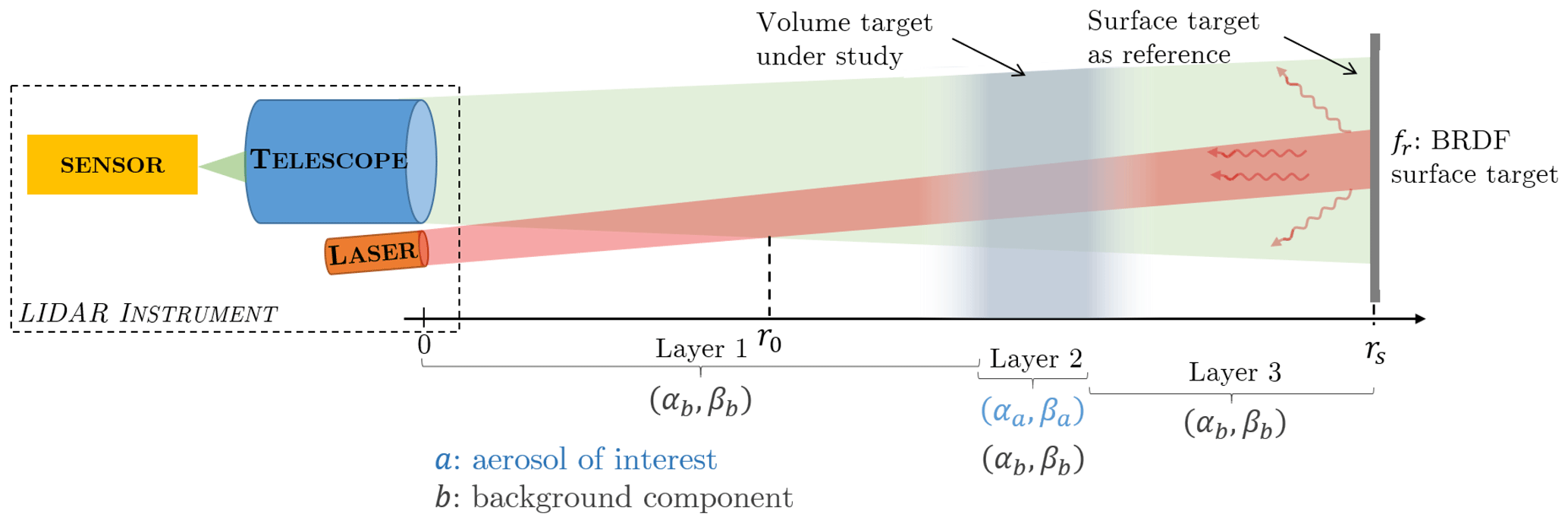
Currently, lidar inversion methods use a volumetric layer of the upper atmosphere (higher than an altitude of 8 km above ground level) as a reference target. This volume is considered as being free of aerosols and made only of pure molecular constituents whose optical scattering properties are known. In our approach, we propose using a SRT of known bidirectional reflectance distribution function (BRDF) f_r,λ (sr⁻¹) (Nicodemus, 1965; Kavaya et al., 1983).

This requires modification of the usual lidar equation in order to make it suitable for both surface and volumetric targets.

For the single-scattering lidar equation, for which light has undergone only one scattering event, the measured backscattered power, at range r, can be written in a general way, viz. by considering both a surface target (Bufton, 1989; Hall and Ageno, 1970) and a volumetric target (Collis and Russell, 1976), as

$$\begin{array}{}\text{(1)}& \begin{array}{rl}{\mathcal{P}}_{\mathit{\lambda }}(r,{\mathit{\theta }}_i)& ={\mathcal{P}}_{\mathrm{p},\mathit{\lambda }}{\displaystyle \frac{c{\mathit{\tau }}_{\mathit{\lambda }}}{\mathrm{2}}}{\displaystyle \frac{A_{\mathrm{ef}}}{r^{\mathrm{2}}}}\left\{{\mathit{\beta }}_{\mathit{\lambda }}\left(r\right)+{\displaystyle \frac{\mathrm{2}}{c{\mathit{\tau }}_{\mathit{\lambda }}}}{f}_{\mathrm{r},\mathit{\lambda }}\right.\\ & \left.(r_{\mathrm{s}},{\mathit{\theta }}_i)F_{\mathrm{cor}}\right\}{T}_{\mathit{\lambda }}^{\mathrm{2}}\left(r\right){\mathit{\xi }}_{\mathit{\lambda }}\left(r\right){\mathit{\eta }}_{\mathit{\lambda }},\end{array}\end{array}$$

where 𝒫_p,λ (W) is the peak power of the laser source, $c\approx \mathrm{3}\times {\mathrm{10}}^{\mathrm{8}}\mathrm{m}{\mathrm{s}}^{-\mathrm{1}}$ is the Einstein constant, τ_λ (s) is the laser pulse duration (full width at half maximum) and A_ef (m²) is the telescope effective receiving area θ_i (rad) the angle between the normal eigenvector to the SRT and the incident beam direction. It should be noted that in the particular case of a Lambertian surface, $f_{\mathrm{r},\mathit{\lambda }}(r_{\mathrm{s}},{\mathit{\theta }}_i)$ can be easily expressed by spectral bidirectional reflectance factor ρ_λ from ρ_λ cos θ_i∕π (Josset et al., 2018, 2010b; Haner et al., 1998). However, the general form of BRDF (f_r,λ) will be considered later in this work in order to not restrict the approach to specific cases. Also, the SRT is located at range r_s, with ξ_λ the dimensionless overlap function and η_λ the dimensionless optical efficiency of the whole receiver. 𝒫_p,λ is a rectangular-shaped pulse in the volumic lidar equation (Measures, 1992), viz. the ratio between the pulse energy and τ_λ. In the case of lidar measurements on a SRT, the backscattered peak power is not proportional to 𝒫_p,λ. A corrective factor F_cor depending on the real shape of the laser pulse is thus introduced. In the present case, ${\mathcal{P}}_{\mathrm{p},\mathit{\lambda }}^{\mathrm{G}}={\mathcal{P}}_{\mathrm{p},\mathit{\lambda }}^{\mathrm{s}}{F}_{\mathrm{cor}}$, with ${\mathcal{P}}_{\mathrm{p},\mathit{\lambda }}^{\mathrm{G}}$ and ${\mathcal{P}}_{\mathrm{p},\mathit{\lambda }}^{\mathrm{s}}$ the peak powers of a Gaussian-shaped and a square laser pulse, respectively. Conservation of the pulse energy between these two kinds of pulses gives $F_{\mathrm{cor}}=\mathrm{2}(\ln \mathrm{2}/\mathit{\pi }{)}^{\mathrm{1}/\mathrm{2}}$ (Paschotta, 2008). The factor does not apply to the volume part of the lidar equation because, in this last part, the pulse profile is assumed to be constant over a rate duration τ_λ. This approximation cannot be made for the backscatter peak of a SRT, because the backscattered energy is not integrated over a volume.

In Eq. (1), $T_{\mathit{\lambda }}^{\mathrm{2}}$ the back and forth atmospheric transmission throughout the environment between the lidar source and range r (Swinehart, 1962) is

$$\begin{array}{}\text{(2)}& T_{\mathit{\lambda }}\left(r\right)=\exp \left[-\underset{\mathrm{0}}{\overset{r}{\int }}{\mathit{\alpha }}_{\mathit{\lambda }}\left(x\right)\mathrm{d}x\right],\end{array}$$

with α_λ (m⁻¹) being the total extinction coefficient at wavelength λ and range r, as ${\mathit{\alpha }}_{\mathit{\lambda }}={\mathit{\alpha }}_{\mathrm{b},\mathit{\lambda }}+{\mathit{\alpha }}_{\mathrm{a},\mathit{\lambda }}$. The subscripts “b” and “a” refer, respectively, to the contribution of the background (molecules and aerosols) and to the contribution of the aerosol volumetric target under investigation. The total backscattering coefficient β (m⁻¹ sr⁻¹) is ${\mathit{\beta }}_{\mathit{\lambda }}={\mathit{\beta }}_{\mathrm{b},\mathit{\lambda }}+{\mathit{\beta }}_{\mathrm{a},\mathit{\lambda }}$, with the same meaning as just above for the subscripts. By definition, the corresponding lidar ratios are LR${}_{\mathrm{b},\mathit{\lambda }}\left(r\right)={\mathit{\alpha }}_{\mathrm{b},\mathit{\lambda }}/{\mathit{\beta }}_{\mathrm{b},\mathit{\lambda }}$ and LR${}_{\mathrm{a},\mathit{\lambda }}\left(r\right)={\mathit{\alpha }}_{\mathrm{a},\mathit{\lambda }}/{\mathit{\beta }}_{\mathrm{a},\mathit{\lambda }}$.

The fundamental quantity measured by the lidar instrument is a voltage V (in volts) which is proportional to the backscattered power as follows: $V_{\mathit{\lambda }}\left(r\right)=R_{\mathrm{v},\mathit{\lambda }}{\mathcal{P}}_{\mathit{\lambda }}\left(r\right)$, where R_v,λ is the detection constant (V W⁻¹) which determines the light–voltage conversion. It can be written using the instrumental constant as follows: $C_{\mathrm{ins}}=R_{\mathrm{v},\mathit{\lambda }}{K}_s$ (V m³), where $K_s={\mathcal{P}}_{\mathrm{p},\mathit{\lambda }}c{\mathit{\tau }}_{\mathit{\lambda }}{A}_{\mathrm{ef}}\mathit{\eta }/\mathrm{2}$. In the literature, C_ins is obtained from 𝒫_λ, while, herein, it comes from the voltage and therefore takes into account all the emission, collection, detection and acquisition chain.

In the sequel, for better readability, the subscript λ and θ_i will not be written thereafter.

The range-corrected lidar signal V_λ(r)r² is as follows:

$$\begin{array}{}\text{(3)}& \begin{array}{rl}S\left(r\right)& =C_{\mathrm{ins}}\left({\mathit{\beta }}_{\mathrm{a}}\left(r\right)+{\mathit{\beta }}_{\mathrm{b}}\left(r\right)+f_{\mathrm{r}}{\displaystyle \frac{\mathrm{2}}{c\mathit{\tau }}}{F}_{\mathrm{cor}}\right)\\ & \exp \left\{-\mathrm{2}\underset{\mathrm{0}}{\overset{r}{\int }}\left[{\mathit{\alpha }}_{\mathrm{a}}\left(x\right)+{\mathit{\alpha }}_{\mathrm{b}}\left(x\right)\right]\mathrm{d}x\right\}.\end{array}\end{array}$$

To remove the α dependence in the exponential term, we will replace α_a and α_b with LR_a and LR_b, respectively, and introduce the term

$$\begin{array}{}\text{(4)}& {\mathrm{LR}}_{\mathrm{a}}\left(r\right)\exp \left\{-\mathrm{2}\underset{\mathrm{0}}{\overset{r}{\int }}{\mathit{\beta }}_{\mathrm{b}}\left(x\right)\left[{\mathrm{LR}}_{\mathrm{a}}\right(x)-{\mathrm{LR}}_{\mathrm{b}}(x\left)\right]\mathrm{d}x\right\},\end{array}$$

as detailed in Ansmann and Müller (2004). With such modifications, the final lidar equation for surface and volumetric scatterers can thus be written as

$$\begin{array}{}\text{(5)}& \begin{array}{rl}S& \left(r\right){\mathrm{LR}}_{\mathrm{a}}\left(r\right)\exp \left\{-\mathrm{2}\underset{\mathrm{0}}{\overset{r}{\int }}{\mathit{\beta }}_{\mathrm{b}}\left(x\right)\left[{\mathrm{LR}}_{\mathrm{a}}\right(x)-{\mathrm{LR}}_{\mathrm{b}}(x\left)\right]\mathrm{d}x\right\}\\ & =C_{\mathrm{ins}}\left[Y\left(r\right)+{\mathrm{LR}}_{\mathrm{a}}\left(r\right){\displaystyle \frac{\mathrm{2}{f}_{\mathrm{r}}}{c\mathit{\tau }}}{F}_{\mathrm{cor}}\right]\exp \left[-\mathrm{2}\underset{\mathrm{0}}{\overset{r}{\int }}Y\left(x\right)\mathrm{d}x\right],\end{array}\end{array}$$

with $Y\left(r\right)={\mathrm{LR}}_{\mathrm{a}}\left(r\right)\left[{\mathit{\beta }}_{\mathrm{b}}\right(r)+{\mathit{\beta }}_{\mathrm{a}}(r\left)\right]$.

Thereafter, in order to highlight the expression to solve, it is convenient to define background-corrected transmission factor as

$$\begin{array}{}\text{(6)}& D(\mathrm{0},r)=\exp \left\{-\mathrm{2}\underset{\mathrm{0}}{\overset{r}{\int }}{\mathit{\beta }}_{\mathrm{b}}\left(x\right)\left[{\mathrm{LR}}_{\mathrm{a}}\right(x)-{\mathrm{LR}}_{\mathrm{b}}(x\left)\right]\mathrm{d}x\right\},\end{array}$$

and W(r)=S(r)LR_a(r)D(r). Finally, Eq. (3) becomes

$$\begin{array}{}\text{(7)}& \begin{array}{rl}W\left(r\right)& =C_{\mathrm{ins}}\left[Y\left(r\right)+{\mathrm{LR}}_{\mathrm{a}}\left(r\right){\displaystyle \frac{\mathrm{2}{f}_{\mathrm{r}}}{c\mathit{\tau }}}{F}_{\mathrm{cor}}\right]\\ & \exp \left[-\mathrm{2}\underset{\mathrm{0}}{\overset{r}{\int }}Y\left(x\right)\mathrm{d}x\right].\end{array}\end{array}$$

We will now introduce the lidar framework adapted to the radiative parameter retrieval of a volumetric scattering medium with a known SRT.

3 New lidar inversion technique

3.1 Radiative parameters identification

The current Klett–Fernald inversion method consists of determining C_ins using the high atmosphere as a reference and fixing the LR_a a priori. In this paper, C_ins is determined by means of a SRT located at range r_s. So,

$$\begin{array}{}\text{(8)}& C_{\mathrm{ins}}={\displaystyle \frac{c\mathit{\tau }}{\mathrm{2}{f}_{\mathrm{r}}{F}_{\mathrm{cor}}}}W\left(r_{\mathrm{s}}\right){\displaystyle \frac{\mathrm{1}}{{\mathrm{LR}}_{\mathrm{a}}\left(r_{\mathrm{s}}\right)}}\exp \left[\mathrm{2}\underset{\mathrm{0}}{\overset{r_{\mathrm{s}}}{\int }}Y\left(x\right)\mathrm{d}x\right].\end{array}$$

It is worth mentioning that LR_a(r_s) is the lidar ratio just before the SRT and Y(r_s)=0 (only at the SRT). Also, obviously, for r<r_s, f_r=0. Inserting Eq. (8) into Eq. (7) gives

$$\begin{array}{}\text{(9)}& W\left(r\right)={\displaystyle \frac{c\mathit{\tau }}{\mathrm{2}{f}_{\mathrm{r}}{F}_{\mathrm{cor}}}}{\displaystyle \frac{W\left(r_{\mathrm{s}}\right)}{{\mathrm{LR}}_{\mathrm{a}}\left(r_{\mathrm{s}}\right)}}Y\left(r\right)\exp \left[\mathrm{2}\underset{r}{\overset{r_{\mathrm{s}}}{\int }}Y\left(x\right)\mathrm{d}x\right].\end{array}$$

This equation applies only before the SRT and can be solved by integrating both sides from r to r_s (Vande Hey, 2014). The exponential term is (see Appendix) as follows:

$$\begin{array}{}\text{(10)}& \exp \left[\mathrm{2}\underset{r}{\overset{r_{\mathrm{s}}}{\int }}Y\left(x\right)\mathrm{d}x\right]=\mathrm{1}+{\displaystyle \frac{\mathrm{4}{f}_{\mathrm{r}}{F}_{\mathrm{cor}}{\mathrm{LR}}_{\mathrm{a}}\left(r_{\mathrm{s}}\right)}{c\mathit{\tau }W\left(r_{\mathrm{s}}\right)}}\underset{r}{\overset{r_{\mathrm{s}}}{\int }}W\left(x\right)\mathrm{d}x.\end{array}$$

Plugging Eq. (10) into Eq. (9), we obtain in the following:

$$\begin{array}{}\text{(11)}& Y\left(r\right)=W\left(r\right){\left[{\displaystyle \frac{c\mathit{\tau }W\left(r_{\mathrm{s}}\right)}{\mathrm{2}{f}_{\mathrm{r}}{F}_{\mathrm{cor}}{\mathrm{LR}}_{\mathrm{a}}\left(r_{\mathrm{s}}\right)}}+\mathrm{2}\underset{r}{\overset{r_{\mathrm{s}}}{\int }}W\left(x\right)\mathrm{d}x\right]}^{-\mathrm{1}}.\end{array}$$

Using the definitions of Y(r) and W(r) (see above), β_a(r) can be written as

$$\begin{array}{}\text{(12)}& \begin{array}{rl}{\mathit{\beta }}_{\mathrm{a}}\left(r\right)& =S\left(r\right)D(\mathrm{0},r)[{\displaystyle \frac{c\mathit{\tau }S\left(r_{\mathrm{s}}\right)D(\mathrm{0},r_{\mathrm{s}})}{\mathrm{2}{f}_{\mathrm{r}}{F}_{\mathrm{cor}}}}+\mathrm{2}\underset{r}{\overset{r_{\mathrm{s}}}{\int }}S(x)\\ & {\mathrm{LR}}_{\mathrm{a}}\left(x\right)D(\mathrm{0},x)\mathrm{d}x{]}^{-\mathrm{1}}-{\mathit{\beta }}_{\mathrm{b}}\left(r\right).\end{array}\end{array}$$

This equation can be written as

$$\begin{array}{}\text{(13)}& \begin{array}{rl}{\mathit{\beta }}_{\mathrm{a}}\left(r\right)& =S\left(r\right)D(r_{\mathrm{s}},r)[{\displaystyle \frac{c\mathit{\tau }S\left(r_{\mathrm{s}}\right)}{\mathrm{2}{f}_{\mathrm{r}}{F}_{\mathrm{cor}}}}+\mathrm{2}\underset{r}{\overset{r_{\mathrm{s}}}{\int }}S(x\left){\mathrm{LR}}_{\mathrm{a}}\right(x)\\ & D(r_{\mathrm{s}},x)\mathrm{d}x{]}^{-\mathrm{1}}-{\mathit{\beta }}_{\mathrm{b}}\left(r\right).\end{array}\end{array}$$

Then, by definition of the lidar ratio, we deduct α_a(r)=LR_a(r)β_a(r). Equation (13) is similar to the one defined by Klett (1981), except that β_b in Eq. (13) also contains the contribution of the aerosol background.

Assuming that the properties of the SRT are well known, the most critical parameter is LR_a(r). Giving a value for LR_a requires a priori knowledge of the volumetric target under study, whereas the main objective of lidar remote sensing is precisely to characterize the medium investigated. A priori information is always a topic of discussions, and it causes more or less severe flaws in lidar measurements.

Equation (13) can also be applied to the important context of airborne observations. In this case, it is necessary to know the ground BRDF.

3.2 Determination of LR_a and β_a: methodology

The objective is to first retrieve β_a(r) and LR_a – and then to deduce α_a(r) – without any a priori knowledge about the medium considered. Two lidar measurements are performed as follows: the first one (signal V_s) in the absence of the volumetric aerosol medium of interest and a subsequent one (signal V_sv) in its presence. The SRT is obviously present for both measurements. The two measurements should be performed close in time in order to avoid the background environment evolving too much. The experimental setup of these lidar measurements is illustrated in Fig. 1.

Figure 1 Illustration of the experimental setup.

By definition, the half-logarithmic ratio of S_s and S_sv corresponds to the total extinction of the volumetric media under study: ${\mathit{\alpha }}_{\mathrm{tot}}=\ln \left[S_s\right(r_{\mathrm{s}})/S_{\mathrm{sv}}(r_{\mathrm{s}}\left)\right]/\mathrm{2}$. Using S_s, C_ins can be determined independently of the volumetric medium of interest as follows:

$$\begin{array}{}\text{(14)}& C_{\mathrm{ins}}={\displaystyle \frac{c\mathit{\tau }}{\mathrm{2}{f}_{\mathrm{r}}{F}_{\mathrm{cor}}}}{S}_s\left(r_{\mathrm{s}}\right)\exp \left[\mathrm{2}\underset{\mathrm{0}}{\overset{r_{\mathrm{s}}}{\int }}{\mathit{\alpha }}_{\mathrm{b}}\left(x\right)\mathrm{d}x\right],\end{array}$$

which is Eq. (8) with α_a=0. C_ins and α_tot are used in objective functions to retrieve LR_a and are assumed to be uniform – r independent. The first objective function is

$$\begin{array}{}\text{(15)}& {\mathit{\epsilon }}_{\mathrm{1}}=\left|\underset{r_{\mathrm{0}}}{\overset{r_{\mathrm{s}}}{\int }}{\mathit{\alpha }}_{\mathrm{a}}\left(x\right)\mathrm{d}x-{\mathit{\alpha }}_{\mathrm{tot}}\right|,\end{array}$$

where α_a is the retrieved profile of extinction using Eq. (13) and LR_a. The medium is assumed to be at a range of full overlap (r>r₀), so that α_tot must correspond to the integrated extinction. A second objective function,

$$\begin{array}{}\text{(16)}& {\mathit{\epsilon }}_{\mathrm{2}}=\left|\underset{r_{\mathrm{0}}}{\overset{r_{\mathrm{s}}}{\int }}\left[S_{\mathrm{sv}}\right(x)-S_{\mathrm{sim}}(x\left)\right]\mathrm{d}x\right|,\end{array}$$

is introduced in order to minimize the difference between S_sv and the simulated signal S_sim obtained from the retrieved β_a and α_a and from C_ins.

The methodology is presented in Fig. 2. The molecular background contribution is computed from pressure and temperature data as in Bucholtz (1995), while the aerosol background contribution is estimated by means of radiative transfer codes, e.g., MATISSE (Simoneau et al., 2002; Labarre et al., 2010) or MODTRAN (Berk et al., 2008, 2014). Another solution consists of using a realistic value of the visibility 𝒱 (km⁻¹) and Koschmieder's relation (Horvath, 1971; Elias et al., 2009; Hyslop, 2009) at 550 nm (maximum human eye sensitivity): 𝒱α_b≈3.9.

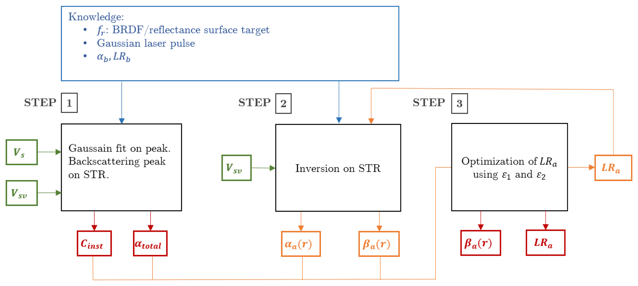
Figure 2 Diagram illustrating how the inversion algorithm allows one to retrieve the β_a(r) and LR_a without assumptions about the volume medium of interest. In green are the lidar signals inputs; in orange are the intermediate calculations during the optimization procedure, and in red are the code outputs.

The signals V_s and V_sv are introduced in the inversion procedure, which is organized around three main steps (Fig. 2):

1. A Gaussian fit is first applied to the backscattered signal from the SRT, i.e., V_s(r_s) and V_sv(r_s), which gives the amplitude of the backscattering, the position of this peak and its width in position. From these Gaussian models, one can obtain α_tot (from its definition; see above) and C_ins from Eq. (14). Note: when the target is tilted with respect to the lidar-target line, the backscatter peak of surface target will not be symmetrical. Another fit should be used as a lognormal function.

2. A first lidar inversion is realized using Eq. (13) with LR_a=50 sr at the beginning of the inversion procedure. This value has been chosen because it corresponds to the average LR_a data from the literature. For that, the Gaussian model V_sv obtained at step 1 is used for signal S(r_s) in Eq. (13). A first range-profile β_a(r) is thus obtained at the end of this second step.

3. The above β_a(r) and LR_a allow us to determine α_a(r) whose r integration is then compared with α_tot in the minimization procedure of Eq. (15). At each iteration, the LR_a is modified in order to reduce ε₁. The new β_a(r), LR_a and α_a(r) values are then used to compute a simulated lidar signal S_sim whose comparison with S_sv is minimized according to Eq. (16). In this algorithm, the iterative procedure ends when ${\mathit{\epsilon }}_{\mathrm{1}}+{\mathit{\epsilon }}_{\mathrm{2}}\le {\mathrm{10}}^{-\mathrm{6}}$ is reached. The use of 19 iterations is generally enough, depending on the first value of LR_a introduced initially (step 2). At the end of this step, one thus obtains final β_a(r), α_a(r) and LR_a. The minimization procedure used is the one implemented by Kraft (1988). Equation (15) is the most important since it determines the rapidity of convergence. Equation (16) is helpful but not critical.

4 Theoretical behavior of the retrieval procedure

4.1 Theoretical lidar signals

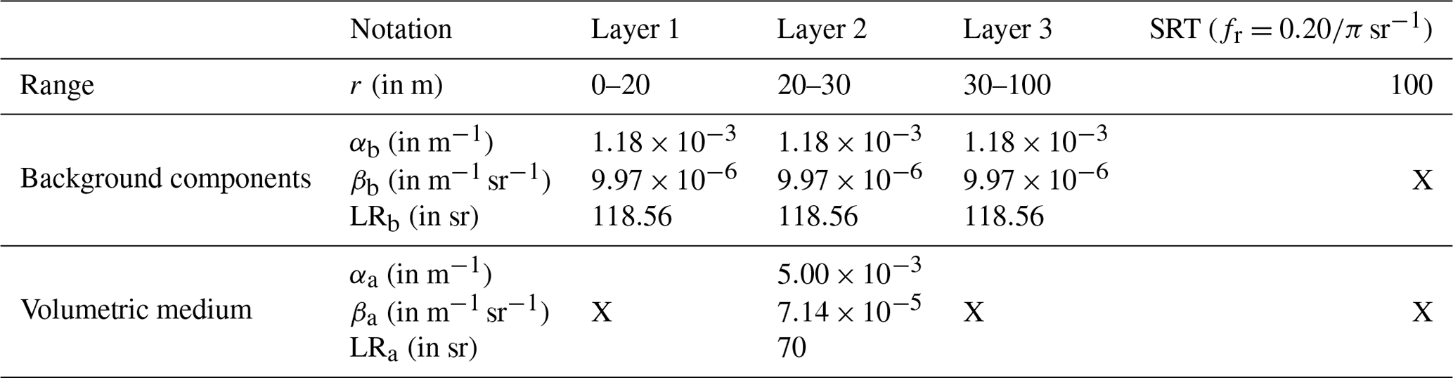
The inversion method described above is tested using theoretical lidar signals generated by PERFALIS (PERFormence Assesment for LIdar Systems; Gaudfrin et al., 2018a). As summarized in Table 1, the simulated atmosphere is composed of three layers and a SRT of BRDF $f_{\mathrm{r}}=\mathrm{0.20}/\mathit{\pi }$ located at r_s=100 m. Pressure and temperature are uniform (1040 hPa and 290 K), and the continental aerosol background is chosen so that it corresponds to 𝒱=47 km (Hess et al., 1998). In addition, ${\mathit{\beta }}_{\mathrm{b}}=\mathrm{9.97}\times {\mathrm{10}}^{-\mathrm{6}}{\mathrm{m}}^{-\mathrm{1}}{\mathrm{sr}}^{-\mathrm{1}}$ and LR_b=118.56 sr. The signal V_s is generated from the background components and the SRT, while the signal V_sv is generated considering an aerosol plume aerosol between 20 and 30 m (second layer). The plume backscatter coefficient is ${\mathit{\beta }}_{\mathrm{a}}=\mathrm{7.14}\times {\mathrm{10}}^{-\mathrm{5}}{\mathrm{m}}^{-\mathrm{1}}{\mathrm{sr}}^{-\mathrm{1}}$ and LR_a=70 sr. Multiple scattering is assumed to be negligible. For dense atmosphere and wider field of view, Eq. (1) has to be corrected by an appropriate factor (Bissonnette, 1996) in order to consider higher orders of scattering events.

Table 1 Input optical parameters of the scene used in the lidar simulator (PERFALIS code) as illustrated in Fig. 1.

Inversion methods are generally applied to averaged signals in order to increase the SNR. In lidar remote sensing, the noise can be, approximately, considered as a white Gaussian noise (Li et al., 2012; Mao et al., 2013; Sun, 2018). In order to assess the impact of noise in the inversion method (see Sect. 3), a Gaussian noise of null mean value and a standard deviation of $\mathrm{1.5}\times {\mathrm{10}}^{-\mathrm{5}}\mathrm{a}.\mathrm{u}.$ is introduced in the theoretical lidar signals. Figure 3 displays the theoretical noised signals V_s and V_sv. As expected, because of light extinction by the plume, V_sv(r_s) is lower than V_s(r_s) by 9 %. Four datasets are then generated, with respectively, an averaging over 20, 50, 100 and 200 signals, from V_s and V_sv, and, in addition, a fifth signal without noise is considered (Fig. 4).

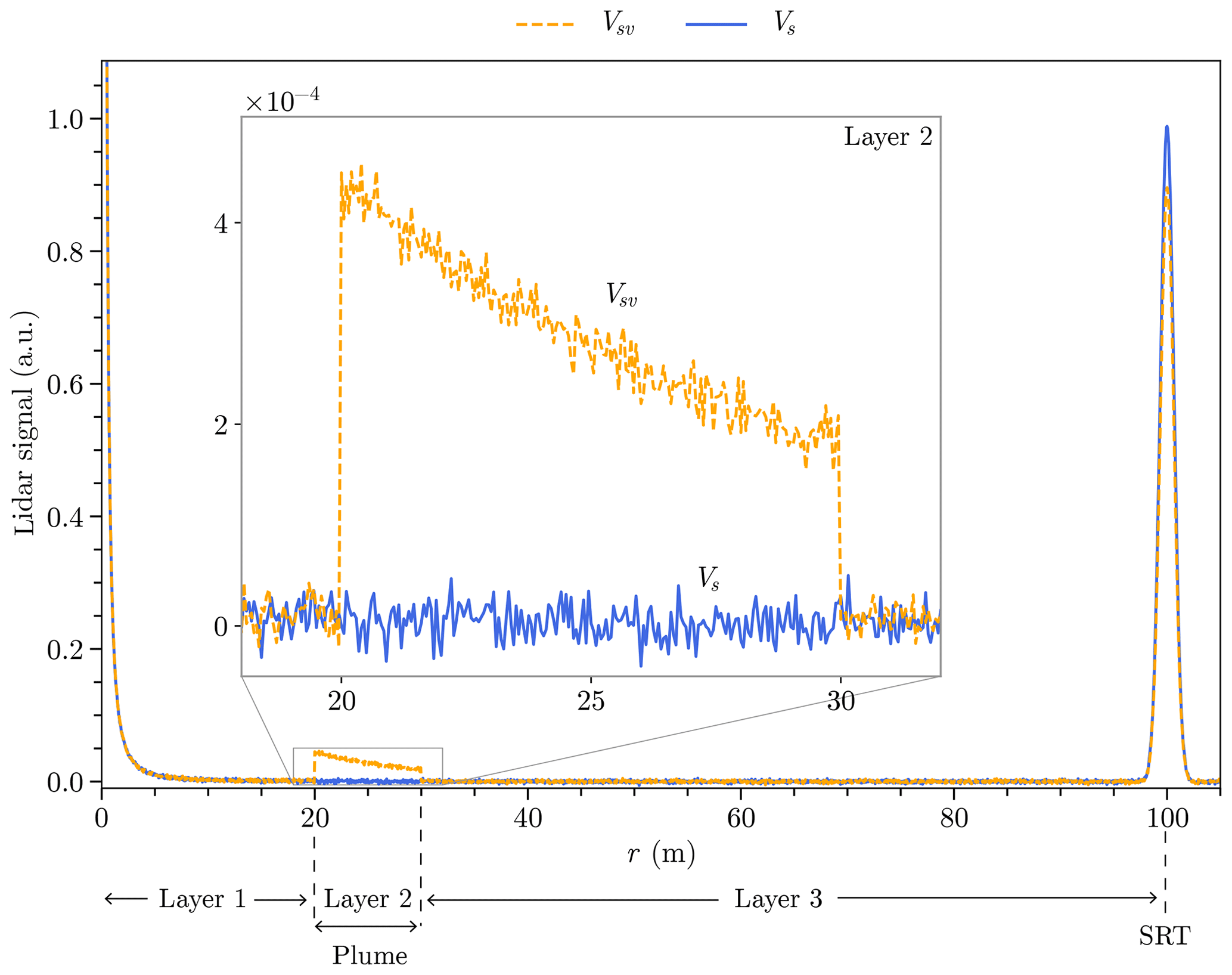
Figure 3 Theoretical noised lidar signals from a SRT V_s (blue line) and in the presence of an aerosol plume V_sv (orange dashed line). Simulations have been performed at 532 nm with molecular and continental aerosol background contributions.

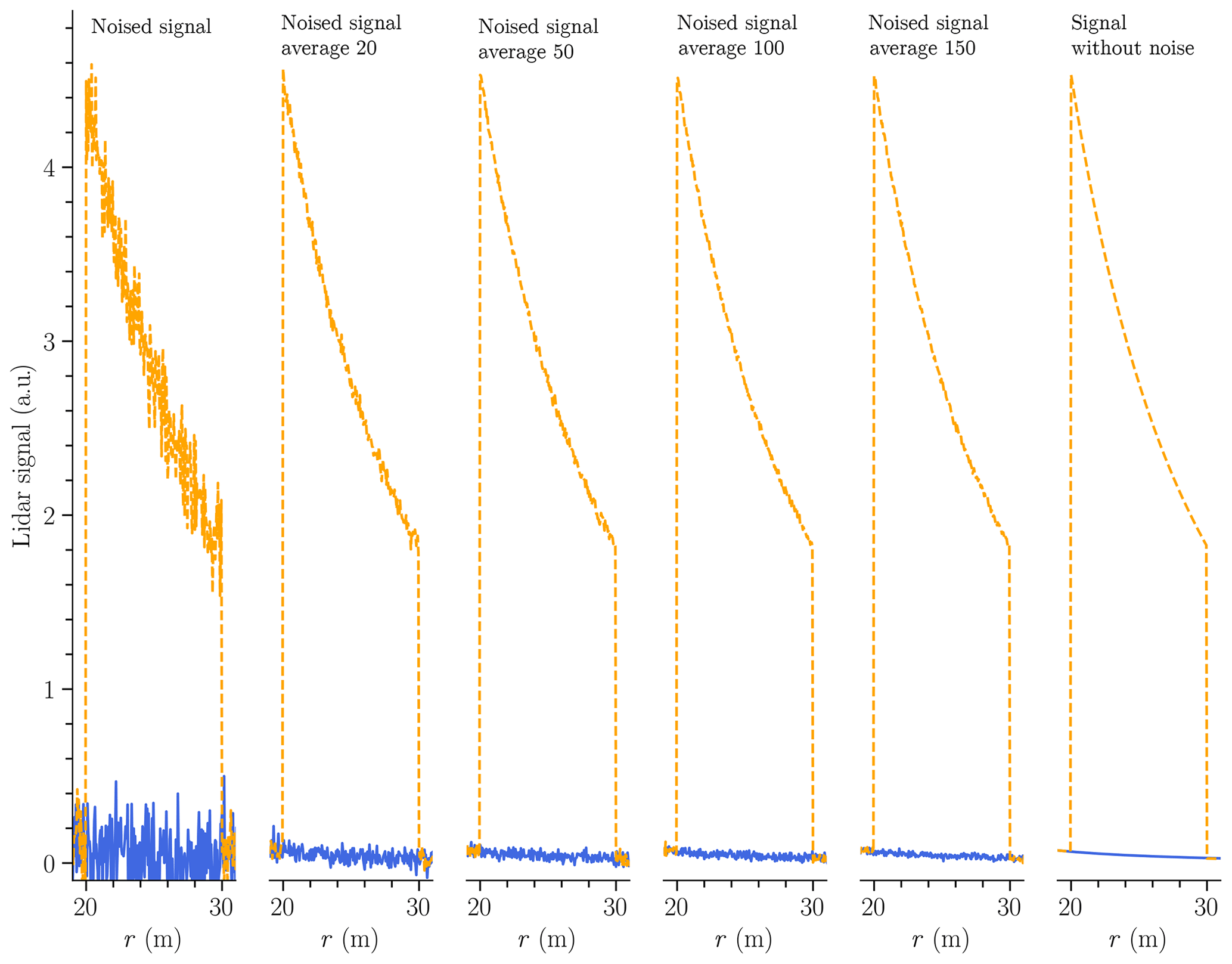
Figure 4 Lidar datasets used in the inversion method. In blue (orange), the lidar signal in the absence (presence) of the volumetric media under study.

4.2 Noise impact on β_a and LR_a retrievals

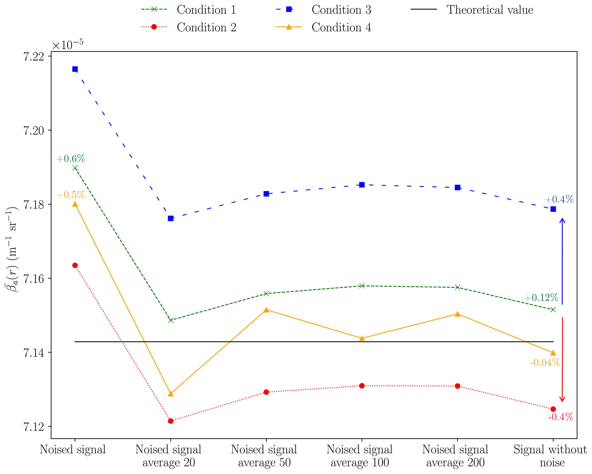
LR_a is retrieved using Eq. (15). In addition to the six-lidar dataset described above, four different conditions of inversion are considered. In condition 1 the exact data of the background components are used as an input in the inversion algorithm. For conditions 2 and 3, β_b is over- and underestimated by 20 % compared to the data used to generate the theoretical signals. In conditions 1 to 3, the inversion technique is performed over the entire signal range. Condition 4 is the same as condition 1, but the aerosol plume is spatially delimited. Table 2 summarizes the four conditions for the six datasets. It is worth mentioning that noised lidar signals obviously result in noised retrieved β_a(r). Thus, to quantify the performance of the inversion technique, we consider the average value $\stackrel{\mathrm{‾}}{{\mathit{\beta }}_{\mathrm{a}}}$ of the plume. The retrieved value of LR_a can be directly compared to the theoretical value.

Figure 5 displays $\stackrel{\mathrm{‾}}{{\mathit{\beta }}_{\mathrm{a}}}$ for the six datasets and the four inversion conditions. It varies from $\mathrm{7.11}\times {\mathrm{10}}^{-\mathrm{5}}$ to $\mathrm{7.22}\times {\mathrm{10}}^{-\mathrm{5}}{\mathrm{m}}^{-\mathrm{1}}{\mathrm{sr}}^{-\mathrm{1}}$, which means an error of approximately 1 % in comparison to the theoretical value. Conditions 2 and 3 result in a translation of the corresponding curve of ±0.4 % with respect to the curve associated with condition 1 because of the over- and underestimation of 20 % introduced in β_b. The performance is better for condition 4 whatever the dataset is, since the maximum error is 0.5 % for noised signals. The spatially bounded aerosol layer is often applied in inversion methods and seems to herein improve the inversion method.

For signal lidar without noise, ${\stackrel{\mathrm{‾}}{\mathit{\beta }}}_{\mathrm{a}}$ is not exactly equal to the theoretical value, maybe because of numerical computation errors in the inversion algorithm. Such a numerical error is about 0.12 % (condition 1) and 0.04 % (condition 4).

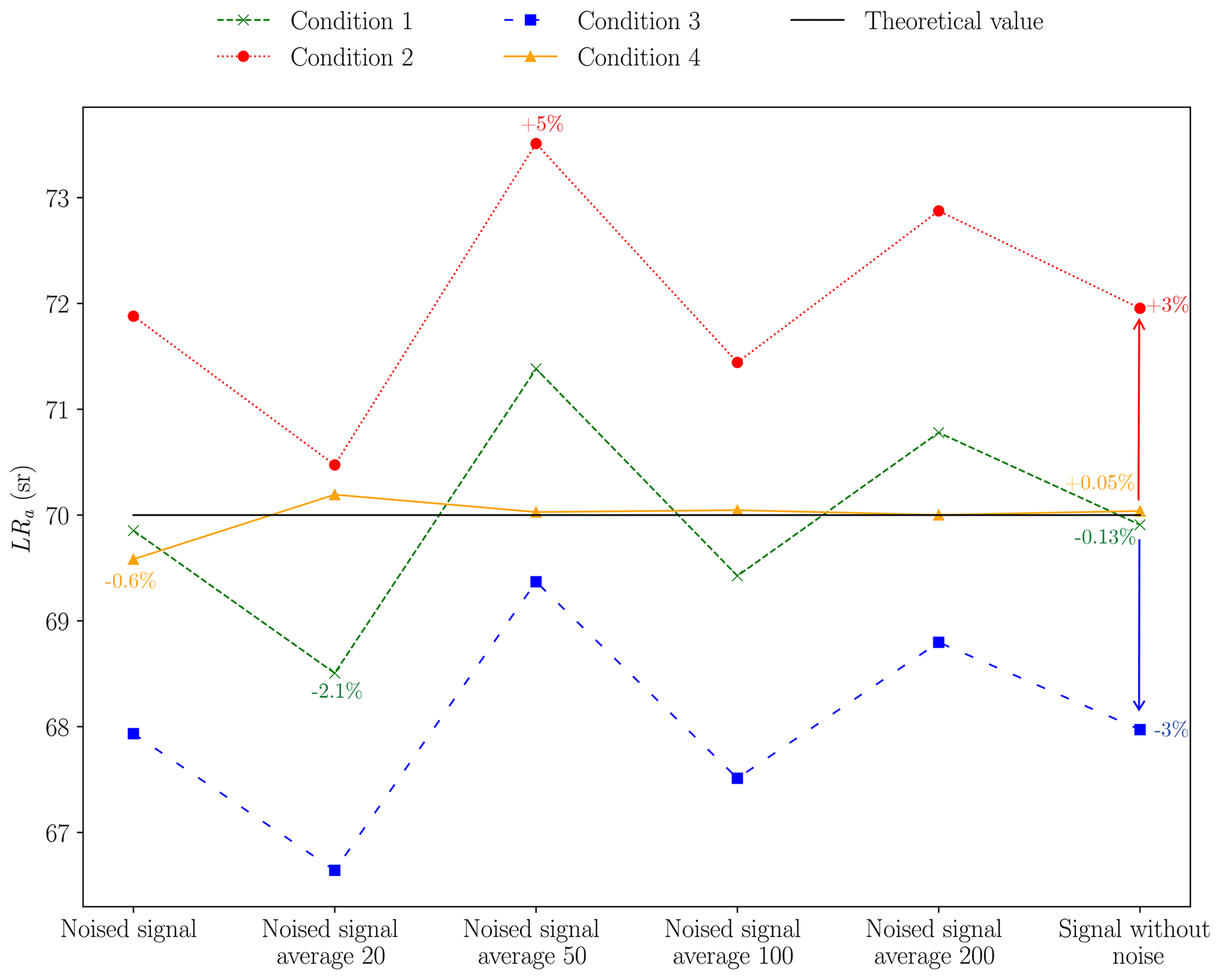
Figure 6 is similar to Fig. 5 but considers LR_a. One obtains values ranging from 66 to 74 sr, with a maximum error of 5 % compared to the theoretical value. In conditions 1, 2 and 3, using averaged noised signals has no consequence on the retrieved value of LR_a, contrary to what was obtained for ${\stackrel{\mathrm{‾}}{\mathit{\beta }}}_{\mathrm{a}}$.

In condition 1, the maximum error is 2.1 %. The graphs corresponding to conditions 2 and 3 are translated with respect to the graph under to condition 1 by about ±3 % and permuted by the same but for ${\stackrel{\mathrm{‾}}{\mathit{\beta }}}_{\mathrm{a}}$. Nevertheless, the errors remain low with a maximum of 5 % (condition 2) if 50 signals are averaged. However, under condition 4, the LR_a is much better for averaged signals and remains quite good for the noised signal (not averaged) with an error rate of 0.6 %. Again, it seems that the spatial limitation of the plume increases the accuracy of the retrieval LR_a. Condition 1 remains, however, efficient for noised signals since deviation is below 2.1 %. In the case of the lidar signal without noise, the retrieved LR_a values are not exactly equal to the theoretical LR_a values; numerical computation errors are about 0.13 % (condition 1) and 0.05 % (condition 4). An error of ±20 % in β_b introduced initially will result in an under- or overestimation LR_a by ±3 %. Condition 4 is preferable for retrieving LR_a.

Figure 5 Retrieved ${\stackrel{\mathrm{‾}}{\mathit{\beta }}}_{\mathrm{a}}$ for six datasets and four different conditions of inversion.

Figure 6 Retrieved LR_a for six datasets and four different conditions of inversion.

Note that the formalism and methodology adopted here to retrieve the lidar ratio are efficient as long as the peak backscattering of the SRT is present on the lidar signal. The method has been evaluated, in this paper, for short range, around 100 m, because our research focus on application at this range. However, the algorithm developed does not present any limit with respect to the range provided that measurements are made below 1 km of range (this value depends of the power of laser sources) with respect to our applications. However, at first sight there is no limit to the application of the method for measurements at longer ranges such as those at more than 1 km.

4.3 Plume optical property retrieval

The above study allowed us to test the new inversion method on noised signals, for different conditions of inversion, as a function of the number of signals averaged. Thereafter, lidar inversion was performed by considering a spatially bounded plume and 100 signals for averaging. This last condition has been chosen because it corresponds to the number of signals available in less than 0.1 s with our lidar system (see Sect. 5). The theoretical results obtained by the inversion method with 100 averaged signals is also quite good (see above). Figure 7 displays the retrieved β_a if a theoretical lidar signal is introduced as a first guess. Table 3 lists the retrieved ${\stackrel{\mathrm{‾}}{\mathit{\beta }}}_{\mathrm{a}}$ and LR_a. Compared to theoretical values, errors are less than 0.7 % for LR_a and below 0.1 % for ${\stackrel{\mathrm{‾}}{\mathit{\beta }}}_{\mathrm{a}}$, although a peak of 2.2 % is observed at r=28.8 m.

Table 2 Conditions placed on the optical properties of the background components for the inversion method.

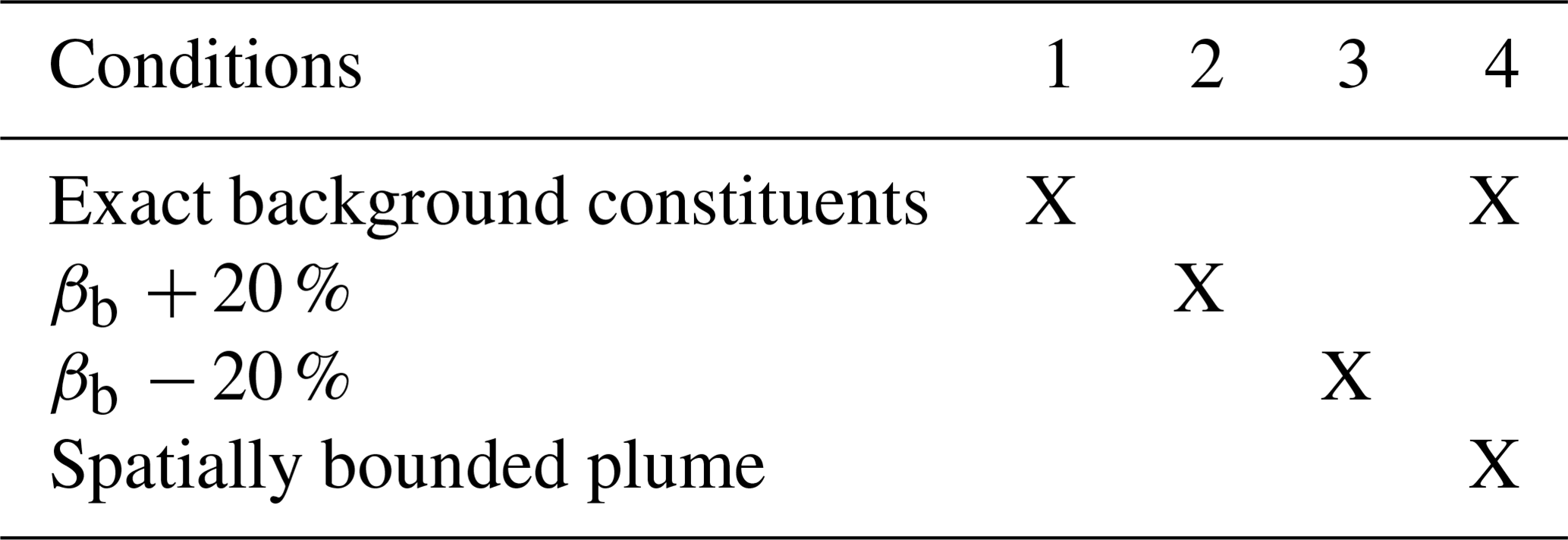
Table 3 Plume optical property retrieved and associated errors.

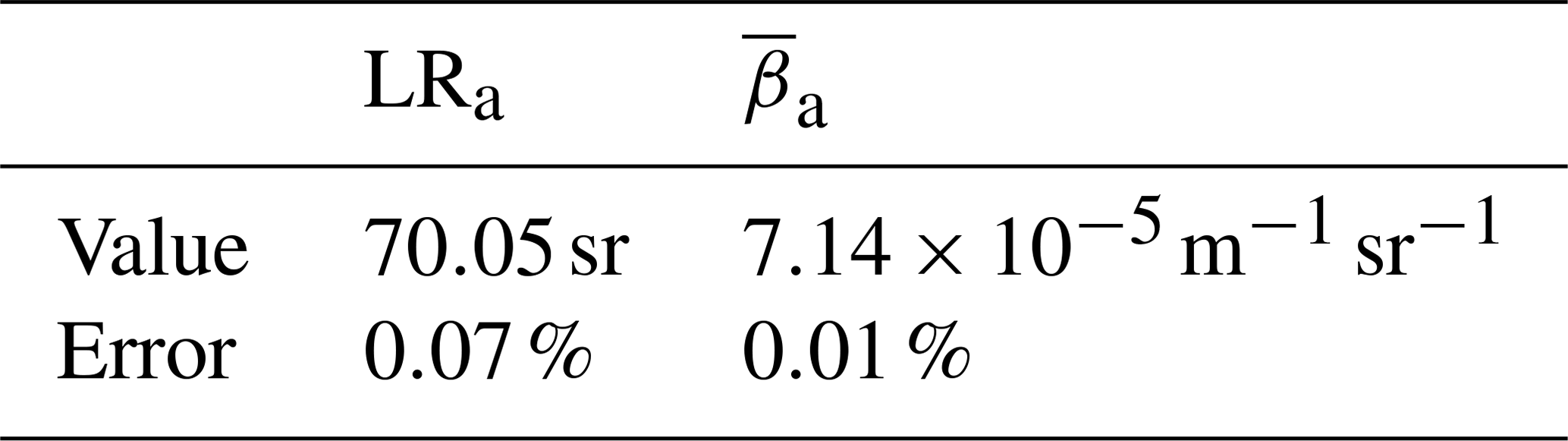
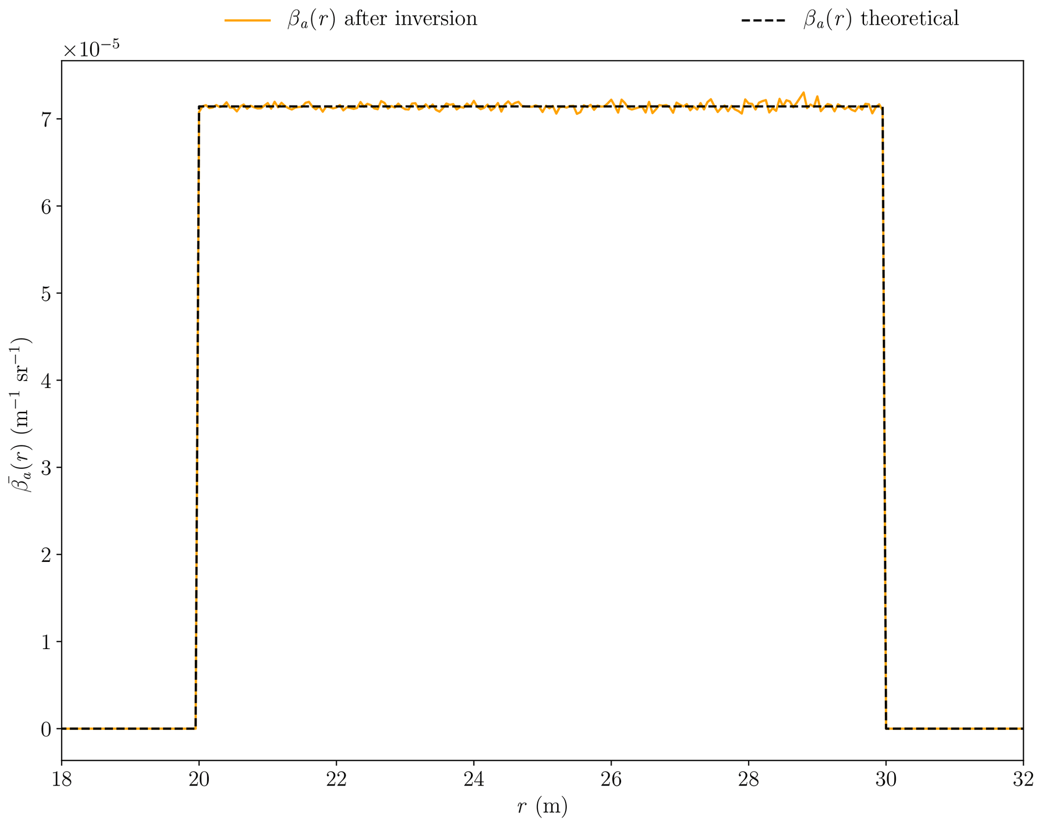
Figure 7 Retrieved β_a(r) (orange solid line) for 100 theoretical averaged lidar signals and initial β_a(r) (dark dashed line).

5 Case of real measurements

Our new inversion technique is now applied to real lidar measurements. The instrument used is named COLIBRIS (COmpact LIdar for Broadband polaRImetric multi-Static measurements; Gaudfrin et al., 2018b; Ceolato and Gaudfrin, 2018). This lidar is able to perform short-range measurements (r₀<5 m) at high spatial resolution (lower than 0.25 m). A Nd:YAG microchip laser source from HORUS, part of the LEUKOS company, is used with a pulse energy peaking at 532 nm of 7.3 µJ and a repetition rate of 1 kHz. The backscattered light is collected by a Cassegrain telescope. In the detection part, a dichroic filter for the elastic channel is used before a photomultiplier tube. The signal is digitized at a sample frequency of 3 GHz after being amplified.

5.1 Description of the experimental operations

The lidar measurements are performed horizontally as illustrated in Fig. 8. A Lambertian Zenithal SRT (SphereOptic, 2020) with a $f_{\mathrm{r}}=\mathrm{0.20}/\mathit{\pi }$ is placed 52 m away from the source. Its spectral bidirectional reflectance has been checked using laboratory bench measurements (Ceolato et al., 2012). The mean direction of the laser beam is parallel to the normal of the surface.

The repetition laser source has repetition frequency of 1 kHz. In order to increase the SNR, we preprocess the measurements from three lidar measurements:

• signal 1 – the first measurement is made by occulting the emitted laser beam to get a measure of the background scene (contribution of passive illumination);

• signal 2 – the second measurement is made by occulting the telescope to estimate the dark noise of the instrument;

• signal 3 – the last measurement is made without any occultation.

Figure 8 Experimental setup in a horizontal configuration. A fog-oil plume is generated between the lidar and the Lambertian SRT. (a) Photo and (b) illustration of the experimental setup with fog-oil plume.

For a given acquisition period, these three series of measured signals are averaged. The averaged signals of the background radiation and the dark noise (signals 1 and 2) are then subtracted from the signal 3 as follows: signal 3 − signal 2 − (signal 1 − signal 2).

Figure 9 shows the lidar results on a volume/surface target over a period of 2 s. This corresponds to 2000 signals per series of measurements. During this period, we assume that the environment does not evolve significantly. The curves V_sv and V_s are the measurements in the presence and in the absence of oil smoke with SRT, respectively. The oil plume signal is visible between 37.5 and 41 m.

The high-speed sampling allows a measurement every centimeter along the line of sight. Combined with a short pulse duration of the laser source (1.7 ns), this makes it possible to highlight local variation concentrations on the order of 25 cm inside the plume with the presence of two maxima at 38 and 39 m from lidar. The peak of backscattering of the SRT is also well sampled. The signal amplitude corresponding to the backscatter of the SRT is lower for V_sv than for V_s because of the presence of the oil plume.

During measurement, the pressure, temperature and visibility are respectively 1016 hPa, 288 K and 30 km. These data are used to compute β_b as described in Sect. 4.

Figure 9 Lidar measurements of the experimental setup. In blue, (orange) the lidar signal in the absence (presence) of the oil-fog plume under study.

5.2 Optical property retrieval: fog-oil plume

The signals V_s and V_sv are used in the inversion procedure as described in Sects. 3 and 4. The plume is spatially bounded (condition 4).

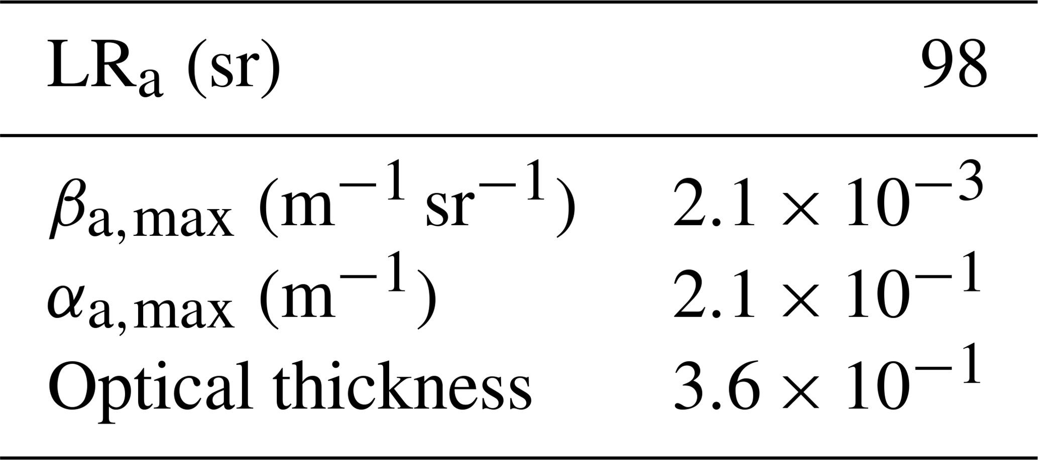
The retrieved β_a(r) is displayed in Fig. 10. In the densest range of the plume ${\mathit{\beta }}_{\mathrm{a}}\approx \mathrm{2}\times {\mathrm{10}}^{-\mathrm{3}}{\mathrm{m}}^{-\mathrm{1}}{\mathrm{sr}}^{-\mathrm{1}}$. Also, the retrieved LR_a is around 98 sr. According to Bohlmann et al. (2018), this value corresponds, as expected, to smoke particles (at 532 nm, the lidar ratio ranges from 80 to 100 sr).The optical properties of the oil-fog plume of experimental retrieved with inverse method are summarized in Sect. 4.

The lidar signal reproduced from the retrieved β_a(r), LR_a and the instrumental constant deduced from the Eq. (14) gives a standard deviation from the exact value of $\mathrm{1.5}\times {\mathrm{10}}^{-\mathrm{5}}\mathrm{a}.\mathrm{u}.$ This shows the consistency and reliability of the new inversion method proposed in this paper.

Figure 10 Retrieved β_a(r) for real measurements with LR_a=98 sr.

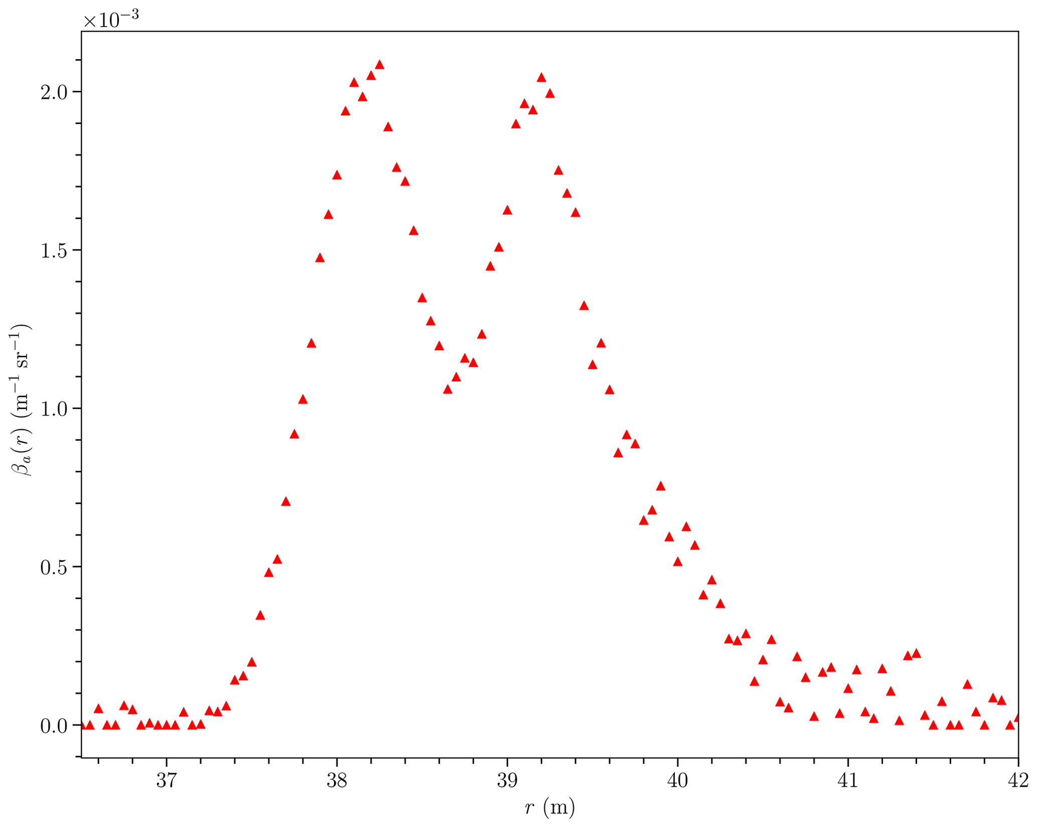
Table 4 Optical properties of oil-fog plume in experimental setup at 532 nm.

6 Conclusions

In this paper, a new method has been introduced for lidar measurement inversion in a situation for which a volumetric layer (molecular Rayleigh scatterers) of the high troposphere is not available (e.g., airborne lidar observations, horizontal configuration of measurements). This method is based on a new expression of the lidar equation which allows us to use a surface reference target of a known BRDF instead of a volumetric one. This new formalism permits the inversion of short-range lidar measurements for which conventional inversion techniques cannot directly be applied. Similarly to common inversion techniques, our method requires the introduction of a background component (molecular and particulate contributions) that can either be estimated from radiative models or deduced from measurements of temperature, pressure and visibility conditions.

Also, a new algorithm has been developed to retrieve, without any a priori assumptions relative to the medium to be characterized (aerosol plume), the backscattering coefficient (β_a) and lidar ratio (LR_a) of an aerosol plume between the lidar and the surface target reference. In other words, our technique does not need to introduce a lidar ratio as an input for our inverse algorithm. For that, two lidar measurements are necessary, with and without the aerosol plume under consideration.

Comparing these two signals, one can retrieve the total extinction coefficient of the medium analyzed and the instrumental constant of the lidar instrument. These two pieces of information are used to constrain the inversion algorithm and finally to identify LR_a.

This algorithm has been first investigated using theoretical (simulated) lidar signals. The quality of the retrieval has been assessed by introducing noise in the simulated signals and by considering various conditions of inversion differing, in particular, from one another according to the initial error introduced in the backscattering coefficient of the aerosol background. Thus, the robustness of algorithm has been shown, since in all the cases, the error on the retrieved values (viz. in β_a and LR_a) is less than 5 %. Also, we have found that inversion is better for spatially bounded aerosol plumes.

The inversion algorithm has then been applied to real lidar short-range measurements of an oil-fog plume. The retrieved β_a and LR_a of the plume agree with values found in the literature for smoke-like particles. Moreover, thanks to the determination of the instrumental constant, the measured signal has been computed from the inverted products, and an absolute error of ${\mathrm{10}}^{-\mathrm{5}}\mathrm{a}.\mathrm{u}.$ between the measure and the post-processed simulation has been encountered.

However, it is worth mentioning that the method proposed herein to find LR_a has some limitations. Precisely, the sensitivity of the lidar must be sufficient to detect the signal of weakly thick or weakly backscattering plume. Indeed, since measurements are performed in the absence and in the presence of the medium, by means of a hard surface target of reference of known reflectance, the algorithm converges less easily for very weakly diffusing plumes.

The new inversion technique presented in this paper suggests new airborne lidar applications operated at low altitude from aircraft (helicopters, airplanes) but requires a priori knowledge of the reflectance of the SRT.

Even if some models exist for the BRDF of surfaces (Bréon et al., 2002; Lobell and Asner, 2002; Mishchenko et al., 1999), their use seems difficult to implement because of the diversity of encountered surfaces during airborne measurements. Nevertheless, it may be possible to identify the reflectance of the ground surface by means of a spectroradiometer imager (Poutier et al., 2002; Miesch et al., 2005; Josset et al., 2018). The combination of these measurements with the herein proposed inversion method would a priori be complementary to establishing of new methods of calibration for down-looking lidar measurements (spaceborne or airborne lidars). The evaluation of the method proposed in this paper, considering the uncertainty in the target reflectance, has not been performed. It will be the topic of future works.

Appendix A

To solve Eq. (9), the exponential term can be written under another form. The method proposed by Vande Hey (2014) consists of integrating both members of the equation from r to r_s. So,

$$\underset{r}{\overset{r_{\mathrm{s}}}{\int }}W\left(x\right)\mathrm{d}x={\displaystyle \frac{c\mathit{\tau }}{\mathrm{2}{f}_{\mathrm{r}}{F}_{\mathrm{cor}}}}{\displaystyle \frac{W\left(r_{\mathrm{s}}\right)}{{\mathrm{LR}}_{\mathrm{a}}\left(r_{\mathrm{s}}\right)}}\underset{r}{\overset{r_{\mathrm{s}}}{\int }}\left\{Y\left(x\right)\exp \left[\mathrm{2}\underset{x}{\overset{r_{\mathrm{s}}}{\int }}Y\left(r\right)\mathrm{d}r\right]\right\}\mathrm{d}x.$$

Since

$$\begin{array}{rl}{\displaystyle \frac{\mathrm{d}}{\mathrm{d}x}}& \left\{\exp \left[\mathrm{2}\underset{x}{\overset{r_{\mathrm{s}}}{\int }}Y\left(r\right)\mathrm{d}r\right]\right\}=\mathrm{2}\exp \left[\mathrm{2}\underset{x}{\overset{r_{\mathrm{s}}}{\int }}Y\left(r\right)\mathrm{d}r\right]{\displaystyle \frac{\mathrm{d}}{\mathrm{d}x}}\left[\underset{x}{\overset{r_{\mathrm{s}}}{\int }}Y\left(r\right)\mathrm{d}r\right]\\ & =\mathrm{2}\exp \left[\mathrm{2}\underset{x}{\overset{r_{\mathrm{s}}}{\int }}Y\left(r\right)\mathrm{d}r\right]{\displaystyle \frac{\mathrm{d}}{\mathrm{d}x}}\left[F\left(r_{\mathrm{s}}\right)-F\left(x\right)\right]\\ & =-\mathrm{2}Y\left(x\right)\exp \left[\mathrm{2}\underset{x}{\overset{r_{\mathrm{s}}}{\int }}Y\left(r\right)\mathrm{d}r\right],\end{array}$$

where F is the primitive of Y. It ensues that

$$\begin{array}{rl}\underset{r}{\overset{r_{\mathrm{s}}}{\int }}Y\left(x\right)& \exp \left[\mathrm{2}\underset{x}{\overset{r_{\mathrm{s}}}{\int }}Y\left(r\right)\mathrm{d}r\right]\mathrm{d}x=-{\displaystyle \frac{\mathrm{1}}{\mathrm{2}}}{\left\{\exp \left[\mathrm{2}\underset{x}{\overset{r_{\mathrm{s}}}{\int }}Y\left(r\right)\mathrm{d}r\right]\right\}}_r^{r_{\mathrm{s}}}\\ & ={\displaystyle \frac{\mathrm{1}}{\mathrm{2}}}\left\{\exp \left[\mathrm{2}\underset{r}{\overset{r_{\mathrm{s}}}{\int }}Y\left(r\right)\mathrm{d}r\right]-\mathrm{1}\right\}.\end{array}$$

Therefore,

$$\underset{r}{\overset{r_{\mathrm{s}}}{\int }}W\left(x\right)\mathrm{d}x={\displaystyle \frac{c\mathit{\tau }}{\mathrm{4}{f}_{\mathrm{r}}{F}_{\mathrm{cor}}}}{\displaystyle \frac{W\left(r_{\mathrm{s}}\right)}{{\mathrm{LR}}_{\mathrm{a}}\left(r_{\mathrm{s}}\right)}}\left\{\exp \left[\mathrm{2}\underset{r}{\overset{r_{\mathrm{s}}}{\int }}Y\left(r\right)\mathrm{d}r\right]-\mathrm{1}\right\}.$$

Finally, the exponential term becomes

$$\exp \left[\mathrm{2}\underset{r}{\overset{r_{\mathrm{s}}}{\int }}Y\left(r\right)\mathrm{d}r\right]=\mathrm{1}+{\displaystyle \frac{\mathrm{4}{f}_{\mathrm{r}}{F}_{\mathrm{cor}}}{c\mathit{\tau }}}{\displaystyle \frac{{\mathrm{LR}}_{\mathrm{a}}\left(r_{\mathrm{s}}\right)}{W\left(r_{\mathrm{s}}\right)}}\left[\underset{r}{\overset{r_{\mathrm{s}}}{\int }}W\left(r\right)\mathrm{d}r\right].$$