the Creative Commons Attribution 4.0 License.
the Creative Commons Attribution 4.0 License.
 | 21 Apr 2020
Characterization and first results from LACIS-T: a moist-air wind tunnel to study aerosol–cloud–turbulence interactions
Jens Voigtländer
Silvio Schmalfuß
Daniel Busch
Jörg Schumacher
Raymond A. Shaw
Frank Stratmann
The interactions between turbulence and cloud microphysical processes have been investigated primarily through numerical simulation and field measurements over the last 10 years. However, only in the laboratory we can be confident in our knowledge of initial and boundary conditions and are able to measure under statistically stationary and repeatable conditions. In the scope of this paper, we present a unique turbulent moist-air wind tunnel, called the Turbulent Leipzig Aerosol Cloud Interaction Simulator (LACIS-T) which has been developed at TROPOS in order to study cloud physical processes in general and interactions between turbulence and cloud microphysical processes in particular. The investigations take place under well-defined and reproducible turbulent and thermodynamic conditions covering the temperature range of warm, mixed-phase and cold clouds (). The continuous-flow design of the facility allows for the investigation of processes occurring on small temporal (up to a few seconds) and spatial scales (micrometer to meter scale) and with a Lagrangian perspective. The here-presented experimental studies using LACIS-T are accompanied and complemented by computational fluid dynamics (CFD) simulations which help us to design experiments as well as to interpret experimental results.
In this paper, we will present the fundamental operating principle of LACIS-T, the numerical model, and results concerning the thermodynamic and flow conditions prevailing inside the wind tunnel, combining both characterization measurements and numerical simulations. Finally, the first results are depicted from deliquescence and hygroscopic growth as well as droplet activation and growth experiments. We observe clear indications of the effect of turbulence on the investigated microphysical processes.
- Article
(5771 KB) - Full-text XML
- BibTeX
- EndNote


Clouds are important players in both weather and climate. They are the source of precipitation and significantly contribute to the radiative budget of the Earth (Lamb and Verlinde, 2011). Extensive research activity during the last decades has been carried out in order to understand cloud processes and related interactions (Mason and Ludlam, 1951; Hobbs, 1991; Kreidenweis et al., 2019). As a consequence, the quantitative knowledge has increased tremendously in the past decades but many of the occurring interactions and their influence on weather and climate are still poorly understood and ill quantified (Quaas et al., 2009; Seinfeld et al., 2016; Kreidenweis et al., 2019).
Atmospheric clouds are often nonstationary, inhomogeneous, intermittent, and cover an enormous range of spatial (micrometers to hundreds of kilometers) and temporal (microseconds to hours and days) scales with cross-scale interactions between turbulent fluid dynamics and cloud microphysical processes influencing cloud behavior and cloud development (Bodenschatz et al., 2010). Turbulence drives processes such as entrainment and mixing, leading to strong fluctuations in aerosol particle concentration, temperature, water vapor and consequently supersaturation with implications for cloud droplet activation, growth and decay (Siebert et al., 2006; Chandrakar et al., 2016; Siebert and Shaw, 2017). Indeed, it has been shown that representation of unresolved fluxes in large-eddy simulations influences properties of simulated stratocumulus clouds (Shi et al., 2018) and that the range of scales captured in direct numerical simulations of cloud entrainment influence the width of the droplet size distribution (Kumar et al., 2018). Even without the presence of strong entrainment, fluctuations in supersaturation can influence the functional form of the cloud droplet size distribution (e.g., McGraw and Liu, 2006; Chandrakar et al., 2016, 2020; Saito et al., 2019). Turbulence also influences particle collision rates and is therefore thought to be central to precipitation formation (Shaw, 2003; Wang and Grabowski, 2009). These processes, in turn, can have buoyancy and drag effects on turbulence and influence cloud dynamic processes up to the largest scales (Stevens et al., 2005; Malinowski et al., 2008; Bodenschatz et al., 2010).
The remote location (high above the ground) and transience of clouds makes comprehensive characterization of clouds and their environment very difficult. Moreover, the intermittent nature of clouds requires the observation of a large number of clouds before statistics will converge. The study of atmospheric clouds is therefore an ambitious, expensive and technically challenging undertaking (Stratmann et al., 2009). In order to better understand and quantify the behavior of clouds in general, and the interactions between turbulence and cloud microphysical processes in particular, atmospheric observations alone are far from sufficient, and intensive laboratory investigations under well-defined and reproducible conditions form an irreplaceable part of cloud research (List et al., 1986; Stratmann et al., 2009; Kreidenweis et al., 2019).
A number of laboratory facilities for aerosol and cloud research, such as aerosol–cloud chambers, continuous-flow systems, wind tunnels and electrodynamic balances have been developed and used over the last decades for atmospheric research (a detailed compilation of, and references for, atmospheric chambers and facilities is given in Chang et al., 2016, and Cziczo et al., 2017). At TROPOS, we developed the laminar flow tube LACIS (Leipzig Aerosol Cloud Interaction Simulator; Stratmann et al., 2004; Hartmann et al., 2011) which has been applied for the investigation of aerosol–cloud interaction processes under controllable and reproducible conditions in a continuous-flow setting. Investigations using LACIS comprised the consistent descriptions of both hygroscopic growth and droplet activation for various inorganic (Wex et al., 2005; Niedermeier et al., 2008) and organic materials such as HULIS (humic-like substances; Wex et al., 2007; Ziese et al., 2008), secondary organic aerosol (Wex et al., 2009; Petters et al., 2009) and soot particles (Henning et al., 2010; Stratmann et al., 2010). Further, LACIS has been used for the investigation and quantification of the immersion freezing behavior of mineral dust (Niedermeier et al., 2010; Augustin-Bauditz et al., 2014; Hartmann et al., 2016), ash (Grawe et al., 2016, 2018) and biological particles (Augustin et al., 2013; Hartmann et al., 2013).
These results and those of other laboratory chambers and facilities have been fundamental in filling gaps in the big puzzle of understanding aerosol–cloud interactions (Chang et al., 2016). However, the investigations at LACIS and many of those at other facilities were carried out having average and/or slowly changing thermodynamic conditions in the vicinity of the particle/droplet, i.e., neglecting possible influences of turbulent fluctuations in these properties. Only very few experimental setups are available so far for laboratory investigations of aerosol–cloud–turbulence interactions due to the demanding experimental requirements regarding the accuracy and reproducibility of the experimental parameters (e.g., temperature, humidity, particle properties, turbulence parameters). One example is the Pi chamber, which is a turbulent aerosol–cloud reaction chamber studying cloud processes on timescales of minutes to hours (Chang et al., 2016).
In the scope of this paper, we introduce a turbulent moist-air wind tunnel, called LACIS-T (Turbulent Leipzig Aerosol Cloud Interaction Simulator), which has been developed at TROPOS in order to study cloud physical processes in general and interactions between turbulence and cloud microphysical processes, such as droplet and ice crystal formation, in particular. The investigations take place under well-characterized and reproducible turbulent and thermodynamic conditions covering the temperature range of warm, mixed-phase and cold clouds (). The continuous-flow design of the facility allows for the investigation of processes occurring on small temporal (up to a few seconds) and spatial scales (micrometer to meter scale) and with a Lagrangian perspective, in contrast to other facilities like the Pi chamber. A specific benefit of LACIS-T is the well-defined location of aerosol particle injection directly into the turbulent mixing zone as well as the precise control of the respective initial and boundary flow velocity and thermodynamic conditions.
The experimental studies using LACIS-T on aerosol–cloud–turbulence interactions are accompanied and complemented by computational fluid dynamics (CFD) simulations which help us to design experiments, i.e., obtain suitable experimental parameters, as well as to interpret experimental results. The simulations are performed in OpenFOAM® for modeling flow, heat and mass transfer as well as particle and droplet dynamics. In that context we formulated an Eulerian–Lagrangian approach so that the growth of individual cloud particles can be tracked along their trajectories through the simulation domain (see e.g., Kumar et al., 2018).
In the following, LACIS-T and the currently available instrumentation will be described (Sect. 2). The numerical model and boundary conditions as well as the numerical particle tracking method are explained in detail in Sect. 3. Afterwards, we present results concerning the thermodynamic and flow conditions prevailing in LACIS-T, combining both characterization measurements and numerical simulations (Sect. 4). The first results from deliquescence and hygroscopic growth as well as droplet activation and growth experiments are depicted in Sect. 5. Finally, we will close with a summary as well as an outlook concerning cloud microphysical processes we will address with LACIS-T in the near future.
The objective of the wind tunnel design is to generate a locally homogeneous and isotropic turbulent airflow into which aerosol particles can be injected and in which the water vapor saturation is precisely controlled. Under suitable conditions, aerosol particles act as cloud condensation nuclei (CCN) or ice-nucleating particles (INPs) and cloud droplet formation or heterogeneous ice nucleation and subsequent growth within a turbulent environment are observed. The turbulent flow is created as airflows past passive grids, as described in more detail later in this section. The primary novelty of the wind tunnel is the existence of two parallel paths through which air flows and is humidified, which are combined in the turbulent flow region. Because of the nonlinearity of the saturation water vapor pressure on temperature (Clausius–Clapeyron equation), the resulting mixture can be supersaturated. Specifically, the supersaturated environment is created through the generally known process of isobaric mixing (Bohren and Albrecht, 1998). The exact humidity within the turbulent region depends on the temperatures and humidities within the two streams, as well as the location within the turbulent mixing zone in the wind tunnel.
LACIS-T is a closed-loop wind tunnel of Göttingen type (Randers-Pehrson, 1935) which has been designed and built up at TROPOS in collaboration with engineering offices “Ingenieurbüro Dr.-Ing. W. Lorenz-Meyer” and “Ingenieurbüro Mathias Lippold, VDI, Windkanalkonstruktion und Windkanaltechnik”. A schematic of the construction is shown in Fig. 1. The main components are radial blowers, particle filters, valves, flowmeters, the humidification system, heat exchangers, turbulence grids, the measurement section and the adsorption dehumidifying system. These components are applied in order to generate the two particle-free airflows, each of which is conditioned to a certain temperature and water vapor concentration. These two conditioned particle-free airflows are turbulently mixed inside the measurement section, and aerosol particles are injected into the mixing zone of the two particle-free airflows, enabling studies of aerosol–cloud–turbulence interaction performed at ambient pressure. The mean velocity inside the measurement section can be varied between 0.5 and 2 m s−1. The detailed description of LACIS-T's design and its functionality will be given in the following, including the adjustment procedure in terms of the thermodynamic – mainly temperature and water vapor concentration – and flow conditions.

Figure 1A schematic of LACIS-T including photos of individual components (© by Ingenieurbüro Mathias Lippold, VDI; TROPOS). The red arrows indicate the flow direction.
Two radial blowers (NICOTRA-Gebhardt, Germany) separately drive the two dry airflows (flow branches “A” and “B”). Flow rates of up to 6000 L min−1 in each flow branch are possible. Afterwards, each flow passes a particle filter (filter class U16; TROX GmbH, Germany) to remove aerosol particles. Subsequently, a defined amount of water vapor can be added to each of the now particle-free airflows by means of a humidification system. For each flow branch, it consists of three humidifiers made of Nafion (FC600-7000, Perma Pure Inc., USA) being surrounded by water jackets and a bypass where the air remains unhumidified. A pump (Grundfos GmbH, Germany) circulates water through the three Nafion humidifiers (150 L min−1 each), and a reservoir compensates for the water loss due to water vapor transport through the Nafion tubes humidifying the particle-free airflow. Heat exchangers, being connected with thermostats (Huber Unistat 510, Peter Huber Kältemaschinenbau AG, Germany), keep the temperature of the water jackets at a defined value (the temperature accuracy is , with T being the actual temperature (∘C), and the stability of the thermostats is ±0.01 K at −10 ∘C). The humidifiers are used in a counterflow fashion. Pneumatically driven valves (Valtek MaxFlo 3, Flowserve Essen GmbH, Germany) are used to adjust the respective volume flows through the bypass and the humidifiers, and ultrasonic flowmeters (Prosonic Flow, Endress+Hauser AG, Switzerland) are applied to measure the respective volume flow rate with an accuracy of 1.5 % of the reading. Due to the setup it is also possible to (a) ensure measurements under dry conditions bypassing the humidifiers and (b) to mix dry and humidified air in order to reach dew-point temperatures below 0 ∘C since the functionality of the Nafion tubes is limited to a temperature range above the melting point of ice. The dew-point temperature of each branch is monitored downstream of the humidification system by means of dew-point mirrors (DPMs, MBW 973, MBW Calibration, Switzerland), which feature an accuracy of K and a reproducibility of K.
Then, the two airstreams are redirected and passed through diffusers, changing the cross section from circular to rectangular. This is needed for the entrance into the heat exchangers (Wätas Wärmetauscher Sachsen GmbH, Germany). Each heat exchanger contains a coolant, the temperature of which can be adjusted to a defined temperature using thermostats (Huber Unistat 915, Peter Huber Kältemaschinenbau AG, Germany; temperature stability of 0.01 K at −10 ∘C). The temperature can be adjusted between −40 and 25 ∘C with an accuracy of and T being the actual temperature (∘C). The dimension of the heat exchangers has been chosen to be able to cool the airflows down to −40 ∘C without any significant undercooling of the cooling liquid, which would lead to condensation or deposition of water vapor at the inner walls and therefore to a loss of water vapor.
Downstream of the heat exchangers, both particle-free airflows are precisely conditioned in terms of volume flow rate, water vapor content and temperature. Before entering the measurement section, the airflows pass passive square-mesh grids (mesh length of M=1.9 cm, rod diameter drod=0.4 cm and a blockage of σb=30 %) which are situated 20 cm above the measurement section (see Fig. 2). This configuration has been chosen to create turbulence that is approximately isotropic in the center region of the measurement section and is homogeneous in transverse planes.
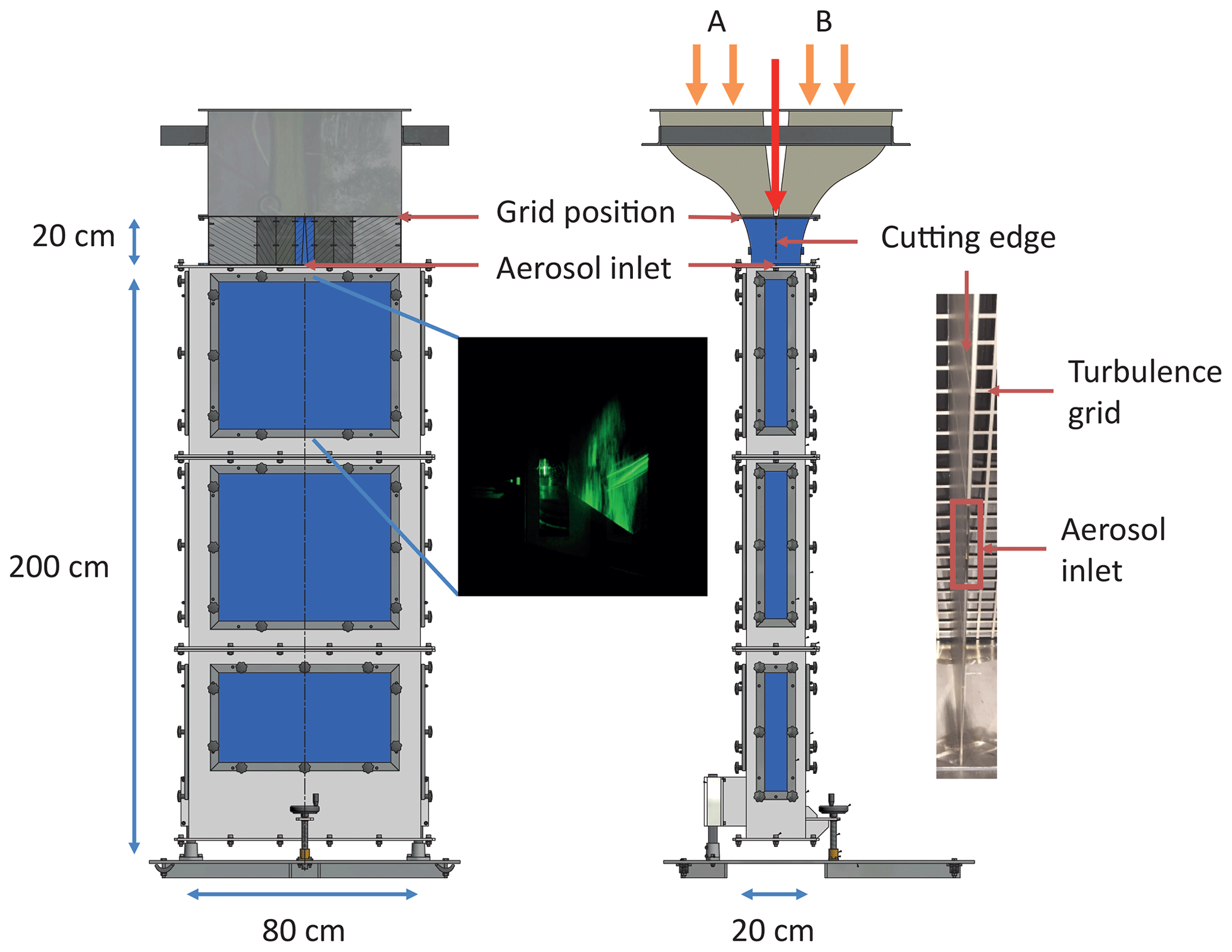
Figure 2A sketch of the measurement section is shown including its dimensions as well as the position of the turbulence grids, the cutting edge and the aerosol inlet (© by Ingenieurbüro Mathias Lippold, VDI; TROPOS). The red arrow marks the location where the particles are injected. The picture in between the sketches of the measurement section shows a formed cloud which is illuminated by a green laser light sheet.
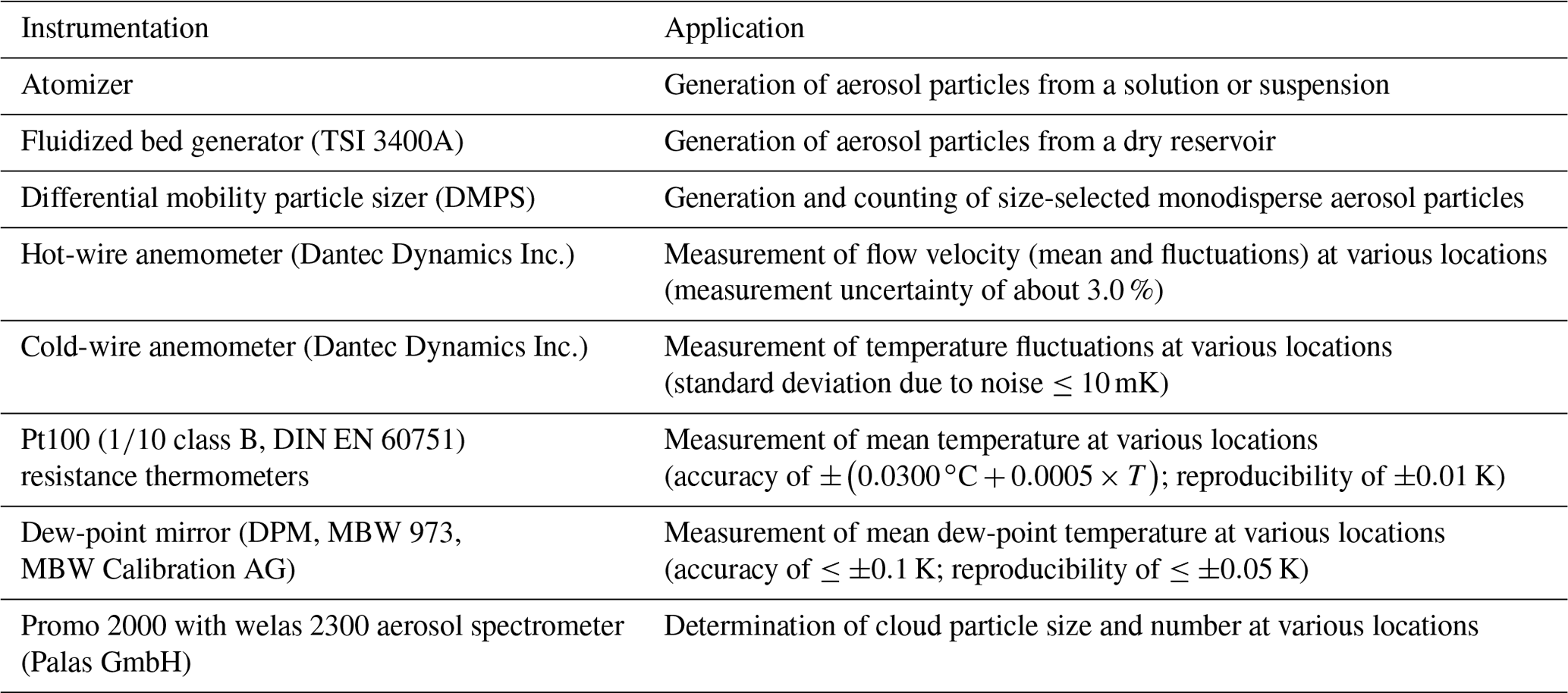
At the inlet of the measurement section, the two conditioned particle-free airflows are merged and turbulently mixed. A wedge-shaped “cutting edge” separates both airflows right above the inlet of the measurement section (see right picture in Fig. 2). Three rectangular feedthroughs, which represent the aerosol inlet (20 mm×1 mm each, 1 mm separation between feedthroughs) are located in the center of this cutting edge. Here, the aerosol flow is introduced into the mixing zone of the two particle-free airflows. Size-selected, quasi-monodisperse aerosol particles of known chemical composition can be injected. Size selection is conducted via a DMPS (differential mobility particle sizer) system which includes a DMA (differential mobility analyzer; Knutson and Whitby, 1975, type “Vienna medium”) for selecting a narrow dry particle size fraction and a CPC (condensation particle counter, TSI 3010, TSI Inc., USA) to obtain the particle concentration. The particles themselves, which can serve as CCN and/or INPs, are generated by means of an atomizer (TSI 3075, TSI Inc., USA) or a fluidized bed generator (TSI 3400A, TSI Inc., USA).
The measurement section itself is a rectangular prism, 200 cm long, 80 cm wide and 20 cm deep (Fig. 2). It features various instruments for characterizing the prevailing thermodynamic, turbulence and microphysical properties. This includes measurements of temperature, mean water vapor concentration, flow velocity, turbulence intensity and dissipation rate as well as cloud particle size distributions at various locations. A summary of the instrumentation available so far is given in Table 1.
The design of the measurement section ensures flexibility in terms of instrument mounting. That means the windows shown in the schematic drawing of the measurement section in Fig. 2 can be replaced by panels with defined positions for access ports as well as customized optical windows. Please note that the measurement section is currently not heat insulated. However, as shown in Sect. 4, wall effects have a negligible influence on the processes occurring in the mixing zone for the experiments carried out so far.
After passing through the measurement section, the entire flow is dried and heated by means of an adsorption dehumidifying system (Marquardt & Schaupp Luftentfeuchtungssysteme GmbH, Germany). Then the flow splits up again into two branches and the whole cycle starts again.
Table 1Available instrumentation for the generation of defined aerosol particles, for the determination of the respective flow, air and dew-point temperature as well as for measuring cloud particle sizes and numbers inside the measurement section.
In summary, we are able to separately adjust and control volume flow rate, temperature and dew-point temperature of each flow branch so that different experimental configurations are possible. This is an important requirement for the experimental studies performed at LACIS-T, especially with regard to our first investigations about deliquescence and hygroscopic growth as well as droplet activation and growth experiments which will be presented in Sect. 5. Two different settings have been applied for these experiments which will be briefly introduced in the following. In the first isothermal setting, both particle-free airflows feature the same conditions in terms of flow rate, temperature and dew-point temperature. The temperature and dew-point temperature of the aerosol flow are adjusted independently of the two particle-free airflows such that microphysical processes like deliquescence and hygroscopic growth of aerosol particles can be studied. In the second non-isothermal setting, the two particle-free airflows are differently conditioned in terms of temperature and dew-point temperature; i.e., there is a temperature difference ΔT between both airflows. If the relative humidities in both airflows are sufficiently high, supersaturation is achieved when both flows are mixed.
As mentioned above, measurements of flow, thermodynamic and cloud particle properties are performed at various locations inside the measurement section. However, it is challenging to determine a comprehensive picture of, for example, the instantaneous parameter fields. Therefore, the experimental investigations are accompanied and complemented by CFD simulations performed in OpenFOAM®. The simulations will further be very helpful for the design of experiments, i.e., obtaining suitable experimental parameters, as well as for the interpretation of experimental results. The simulations will also aid in development of physically sound parameterizations concerning aerosol–cloud–turbulence interaction. In the following the numerical setup for flow and particle dynamics simulations will be presented.
3.1 Computational domain and numerical grid
As already shown, the measurement section is a rectangular prism 200 cm long, 80 cm wide and 20 cm deep. For the simulations, the computational domain comprises only a part of the wind tunnel upstream of the aerosol injection, including the turbulence grid in order to reduce computational effort. It covers the upper 80 cm of the measurement section, and it is 11.5 cm wide and 20 cm deep (Fig. 3). This is the region of interest for the measurements carried out so far. This domain is decomposed into a grid with approximately 7.6×10⁶ cells. Multi-region support, i.e., a coupled simulation of solid and fluid regions, is necessary for non-isothermal setups, as the region between the walls above the aerosol inlet is a solid and thus conducts heat, so that the wall temperature is not fixed but actually depends on the behavior of fluid and solid temperature at the walls. The solid region was decomposed into approximately 30 000 grid cells.
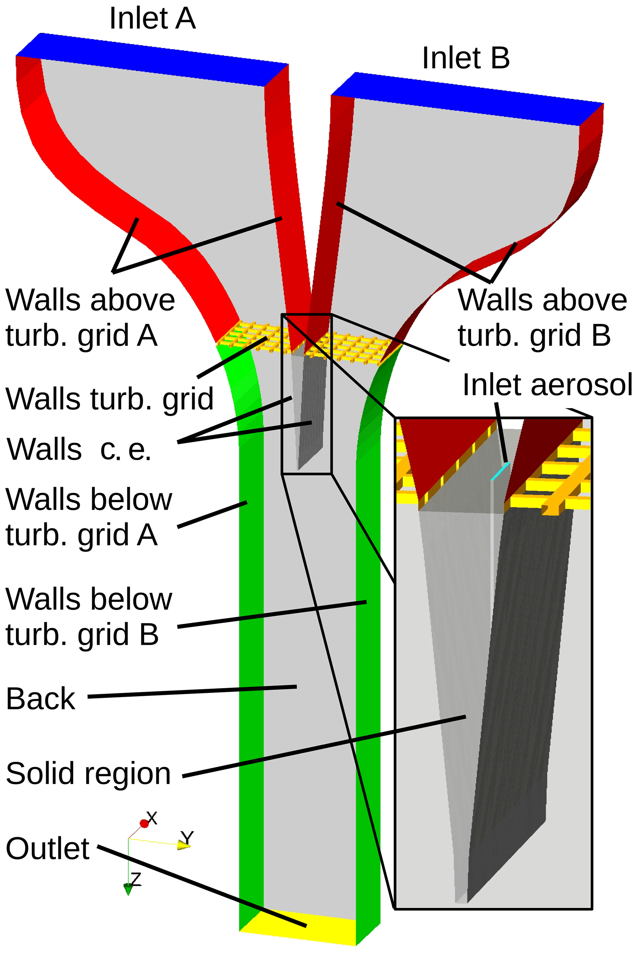
Figure 3Boundaries of the computational domain with detailed view of the aerosol inlet region between the two airflow branches (c.e. stands for cutting edge).
3.2 Fluid flow and heat–mass transfer simulations
For an isothermal (i.e., the temperature in both flow branches A and B is identical, TA=TB), unhumidified (i.e., dry) setup, as will be described in Sect. 4.1, OpenFOAM®'s solver “pimpleFoam” is used, which is a finite-volume solver for incompressible, transient, turbulent flows. Regarding non-isothermal (TA≠TB) and humidified flows, we use an adapted version of OpenFOAM®'s “chtMultiRegionFoam”, which is able to simulate multi-region heat transport and which was extended to also transport the mass fraction of water vapor.
As turbulent fluctuations are to be investigated, it is not suitable to use Reynolds-averaged Navier–Stokes (RANS) models. This would only provide mean values of turbulent properties. A fully resolved simulation (direct numerical simulation, DNS) is far beyond available computational resources but is planned as a possible future work. So the method of choice so far is a large-eddy simulation (LES), calculating the larger, energy-containing eddies and modeling the smallest eddies, so it is not as computationally expensive as a DNS. We choose the dynamic k-equation LES model, as it has proven to be a good model for decaying turbulence and the transport of thermodynamic quantities (Chai and Mahesh, 2012).
The air inside LACIS-T is considered to be an ideal gas with a molar mass of 28.97 g mol−1, a heat capacity of 1.007 kJ (kg K)−1 and a dynamic viscosity of Pa s. Regarding the solid region, approximate properties of steel are used with a molar mass of 56 g mol−1, a thermal conductivity of 40 W (m K)−1, a specific heat capacity of 500 J (kg K)−1 and a density of 8000 kg m−3. Gravitational acceleration is set to 9.81 m s−2 in the vertical direction (positive z direction in Fig. 3).
The different boundary conditions are depicted in Fig. 3 and listed in detail in Table 2. At the inlets, fixed values of velocity, temperature and humidity were set according to measurements (inlet A and inlet B) or set values. The pressure gradient is set to zero.
Table 2Boundary conditions for LES.
a If the value of the water vapor mixing ratio qv exceeds the value which corresponds to a relative humidity (RH) of 100 %, it is set to a fixed value boundary condition, so that RH stays at a maximum of 100 % at the walls. b The region between the left and right sides of the cutting edge is simultaneously simulated as a heat-conducting solid, and the temperatures at the wall are the result of this simulation. c Values according to measurement.
As usual, a no-slip condition for the velocity is assumed at all walls. Wall temperatures have been measured above and below the turbulence grid and the according walls are set to the appropriate values. The turbulence grid is assumed to have approximately the same temperature as the surrounding fluid and thus the temperature gradient is set to zero there. For the humidity, we use a mixed wall boundary condition. For saturated flow conditions, the relative humidity at the wall is set to 100 %. The condensed water is lost and heat release due to condensation is neglected. If the relative humidity at a wall is below 100 %, the gradient is assumed to be zero.
At the outlet, zero-gradient conditions are used for velocity, temperature and humidity. In other words, the respective partial derivate vanishes in the normal direction to the outlet surface. To reduce the computational effort, only a 11.5 cm wide section of LACIS-T was modeled, as mentioned above. At the front and back of this section, periodic boundary conditions are used. Periodic boundary conditions in one or more space directions imply that any fluid field is periodically continued across the domain size in this direction; e.g., the temperature field is periodic in x if with the box length L in x.
The simulations are first run for 1 s of physical time, starting with a steady-state solution, until a quasi-steady state is reached. Afterwards, another 2.5 s of physical time is simulated for statistics. The time step is either fixed at 25 ms, ensuring a maximum Courant–Friedrichs–Lewy (CFL) number of approximately 0.8, or it is adjusted automatically to ensure a CFL number below 0.95. The CFL number is a parameter for the numerical solution of partial differential equations. The discrete time step width Δt in numerical simulations has to be chosen depending on the local velocity magnitude U in the mesh cells and their local widths Δx in order to guarantee the stability of the numerical method. In detail, it should hold . The CFL number is the corresponding dimensionless quantity, . In our case, C should be smaller than 1.
3.3 Particle dynamics simulation
For the particle dynamics simulations, an Eulerian–Lagrangian approach has been chosen. This means that individual particles are tracked along their trajectories through the simulation domain described above. The trajectories are calculated according to the following equations:
Here, xp, Up and mp are the location, velocity and mass of a particle; t is the time; and Fi represents the forces acting on the particle. The forces considered in the present work are the drag force,
and the transverse lift force due to shear lift
with Uf, ρf and ωf being the velocity, density and rotation of the surrounding fluid and ρp and Dp being the particle's density and diameter. The coefficient CD depends on the particle Reynolds number Rep and is usually calculated according to Stokes (1851) for low Rep, and according to Schiller and Naumann (1933) for higher Rep
Rep is calculated with the current values of Dp and the slip velocity |Uf−Up| at every Lagrangian time step:
with νf being the kinematic viscosity of the fluid. As the particles and droplets are rather small (), they are assumed to follow the advecting flow field nearly perfectly; i.e., the slip velocity is small compared to the fluid velocity. Thus, Rep is assumed to be small.
CLS is calculated according to Mei (1992)
with
and with and the Reynolds number of the shear flow
To investigate the particle growth, the particles can gain and lose mass depending on thermophysical properties at their surface:
where ρv, sat is the saturation vapor mass density, S is the ambient water vapor saturation ratio, S* is the water vapor saturation ratio at particle surface (using the Köhler equation; Wilck, 1998) and
is the mass transfer transition function. is the Knudsen number, with λg being the mean free path length of the gas molecules. The parameter α is the mass accommodation coefficient and it is assumed to be 1. For the coefficients A, B1, B2 and C the following values are used: A=1, B1=0.377 and (Fuchs and Sutugin, 1970; Voigtländer et al., 2007). As the concentration of particles used for experiments is currently rather small, only one-way coupling is considered; i.e., the particles' influence on the fluid phase and interactions between them are neglected.
For the particle simulations, the multi-region solver as introduced above is used and extended to include particle tracking, and the domain is also the same as for the characterization simulations. After an initial 1 s of physical time, the particles are injected at the aerosol inlet for another 1 s with a concentration according to the measurements. It is 1000 cm−3 for the droplet activation and growth experiments described later. This leads to about 25 000 particles which are tracked during 3.5 s of real time.
To compare the particle size distributions with their measured counterparts, the size of particles in cylinder-shaped regions in different positions are analyzed for the saved time steps. These cylinders have radii of 7 mm as this is approximately the width of the airstream that enters the welas 2300 spectrometer. The sampled regions are 25 mm long, and their axes coincide with the z axis.
The characterization efforts include measurements of the flow field and the thermodynamic parameters within the measurement section including high-resolution measurements of velocity and temperature (on the decimeter to millimeter (Kolmogorov) scale) as well as measurements of the mean relative humidity. The results will be compared to those of the LES. Overall, the characterization efforts have been performed to ensure the functionality and to investigate the performance of the wind tunnel. Note that the parameter space which can be set within LACIS-T is extensive. Consequently, the characterization efforts presented here will focus on T>0 ∘C conditions as well as on the very first meter of the measurement section with z0=0 cm corresponding to the position of the aerosol inlet which is 20 cm downstream of the turbulence grid.
4.1 Flow properties in the measurement section
The flow field and the turbulent flow properties have been investigated for isothermal (TA=TB) and non-isothermal (TA≠TB) conditions with different dew-point temperature settings inside the measurement section. Here, results will be presented in detail for a dry, isothermal case1; i.e., both airflows featured the same temperature T=20 ∘C and dew-point temperature ∘C. Measurements were performed at various locations underneath the aerosol inlet along the shortest distance of the measurement section by means of the hot-wire anemometer measuring the vertical velocity component at 6000 Hz for 5 min at each location. Measurements were performed for aerosol flow turned-on and turned-off conditions in order to observe the influence of the cutting edge on the flow field. For the simulations, aerosol flow turned-off conditions only have been considered.
In panel (a) of Fig. 4, the simulated time-averaged velocity is shown for two different vertical planes and nine horizontal planes. The two vertical planes show the flow field located underneath the middle of a grid bar of the turbulence grid (left plane) and the middle of the grid openings (right plane). The nine horizontal planes are located at different positions below the aerosol inlet which is at z0. Note that the very first horizontal plane is 1 cm below z0 while the others are located at z1 to z8 with z1=10 cm and Δz=10 cm. Different characteristics of the flow field can be recognized. For example, the expected influence of the “cutting edge” on the flow field can be seen downstream of the aerosol inlet, leading to a decrease in the flow velocity. Further, an increase in the mean velocity is visible close to the side walls, probably caused by the constriction of the cross section leading to an acceleration of the velocity field, which is strongest at the side walls. In the following, these simulation results will be compared to measurement results.
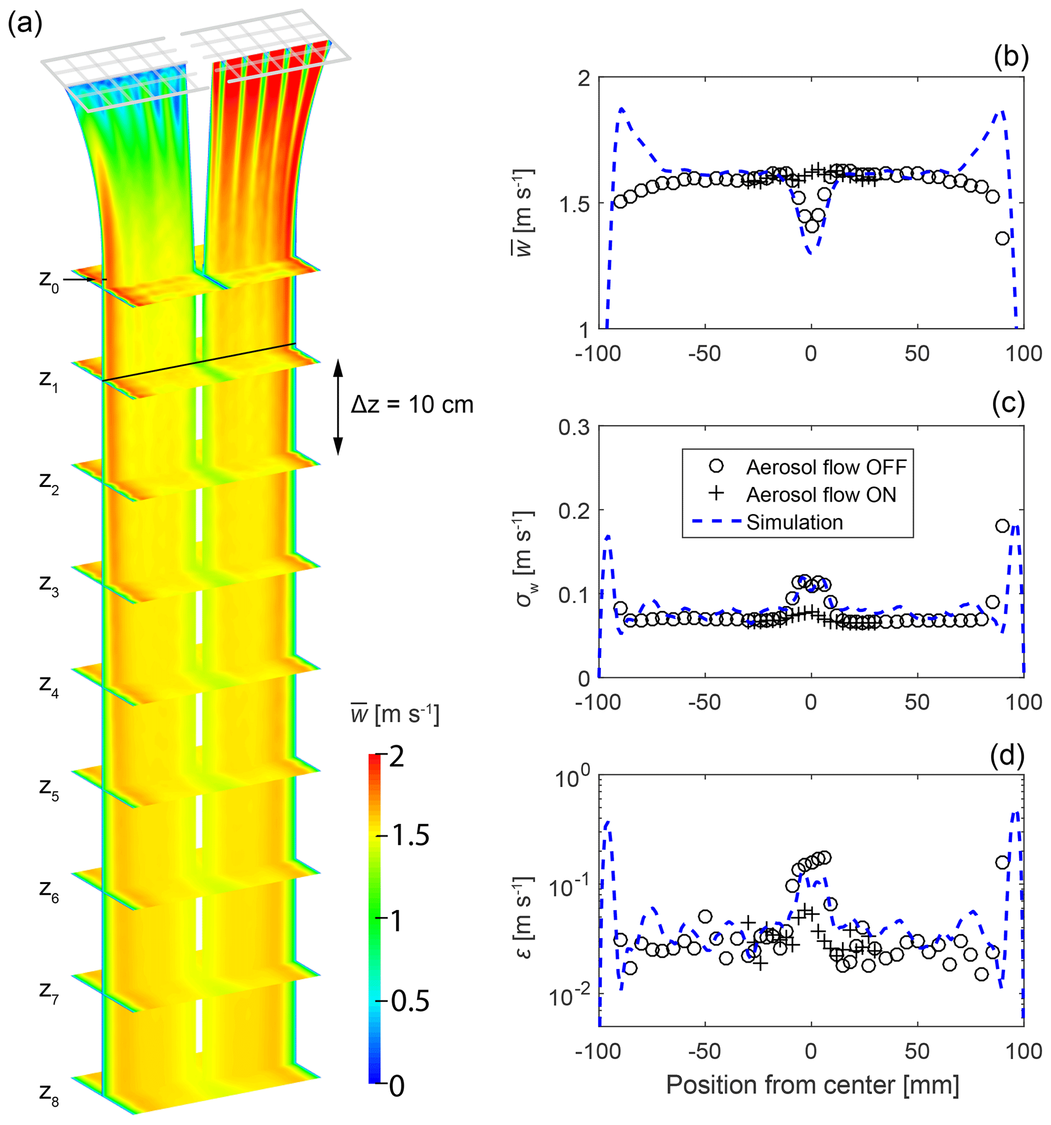
Figure 4(a) Contour plot of the time-averaged velocity in two vertical and nine horizontal planes determined by the LES. The grid is also indicated. Note that the aerosol flow is turned off in the simulations. (b) Profiles of mean velocity , rms velocity σw and energy dissipation rate ε along the center region (black line in (a); position 0 mm corresponds to the center of the measurement section depth, being 100 mm away from each side wall) at z1=10 cm. The results presented are based on hot-wire measurements (at 6000 Hz) performed in the central position of the measurement section underneath the middle of the grid openings. Measurements were taken with turned-on (crosses) and turned-off (open circles) aerosol flow. Corresponding simulation results for and σw are shown as blue dashed lines, for turned-off aerosol flow only.
The plots in panel (b) of Fig. 4 show – from top to bottom – the measured and simulated mean (vertical) velocity , its fluctuation in terms of the root-mean-square (rms) average (with ) and the energy dissipation rate ε obtained at z1. The determination of the energy dissipation rate is based on the relationship
where is the second-order structure function of the vertical velocity component (Wyngaard, 2010), z is the vertical position, r is the separation distance, C=2.1 is the Kolmogorov constant and 〈⋅〉 is the spatial average. We used Taylor's frozen flow hypothesis to transform from temporal space to physical space. The application of this hypothesis is reasonable as .
The mean velocity profile is homogeneous, apart from the areas near the wall of the measurement section and in the center region with the aerosol flow turned off. The increase in the mean velocity close to the side walls is not visible in the measurements, probably due to objects related to the turbulence grid's clamping system (not considered in the simulations), which strongly reduce the acceleration at the walls. Increased turbulence intensities, represented in terms of σw, are observed in the near-wall area due to wall-induced turbulence. Furthermore, shear stresses in the mixing region cause higher turbulence and thus higher fluctuations. By turning on the aerosol flow (isokinetic flow conditions), the inhomogeneity in the center region of the measurement section can be eliminated for both the mean velocity and its fluctuations. Thus these shear effects are strongly decreased in the mixing zone of the two airflows. The dissipation rate is in the range of m2 s−3 in the homogeneous region, which leads to the Kolmogorov time and length scales of s and mm, with m s−2. The integral length l and the Taylor microscale λt are cm and cm. The latter leads to the Taylor–Reynolds number . Reλ is much smaller than the values typically encountered in atmospheric clouds; however, this is not a limitation for studies of small-scale interactions of cloud particles–droplets and turbulence as long as intermittency aspects can be neglected (Siebert et al., 2010; Chang et al., 2016).
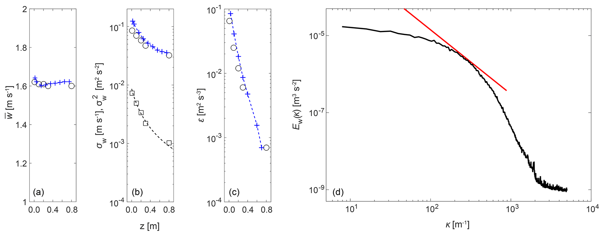
Figure 5The measurements shown in Fig. 4 were carried out for five different heights below the aerosol inlet. The values for mean velocity, rms velocity and dissipation rate are averaged in the range from −70 to +70 mm (switched-on aerosol flow) and are shown in (a, b, c) by the black circles. Panel (b) further shows the drop in turbulent kinetic energy in terms of the squared rms velocity (black squares) which follows a power-law function with an exponent of −1.4 (dotted black line). Additionally, the respective results from the simulations are shown (blue plus signs), also averaged in the range from −70 to +70 mm. The experimentally determined turbulent spectrum for the velocity fluctuations is shown in (d). A red line with a slope is shown as a reference.
Figure 5a–c show the values for , σw and ε for five different distances to the aerosol inlet averaged over the range where the dissipation rate is homogeneous. Looking at the values determined through the measurements, it can be seen that the mean velocity remains almost constant (slight decrease with increasing distance to the aerosol inlet), while the fluctuations and thus also the energy dissipation rate decrease with increasing distance from the turbulence grid. This observed decrease in the turbulent kinetic energy, which is also presented in terms of in Fig. 5b, follows a power-law function , where zgrid represents the grid position. The exponent n is −1.4 and is comparable with results reported in other wind tunnel investigations and depends on the initial conditions (Lavoie et al., 2007, and references therein). Additionally, the simulated values for , σw and ε are given. We observe a slight decrease in until z=0.2 m which is similar to experimental observations. However, it is followed by a slight increase which is in contrast to the measurements. This slight increase in the simulated is caused by the high velocities obtained close to the walls (see Fig. 4), which spread slowly and also reach the inner region. The decrease in σw and ε is well reproduced by the simulations.
The turbulent spectrum for the velocity fluctuations is shown as an example in Fig. 5d. A red line with a slope, which is expected for the inertial subrange of the turbulent energy cascade, is shown as a reference. The inertial subrange is not fully evolved, which is to be expected for Reλ≈30. However, this is not a limitation as turbulence on the small scale is already developed (Schumacher et al., 2007) and our focus will be on small-scale interactions of cloud particles and turbulence.
4.2 Thermodynamic properties in the measurement section
The momentum exchange in turbulent flows is comparable to an increased molecular viscosity. However, the turbulent mixing not only includes momentum but also includes further associated properties such as heat and mass. We performed several characterization experiments to study the turbulent transport of heat and mass in the measurement section. All related studies were performed without the insertion of aerosol particles. The measurements are again accompanied by LES where the inlet conditions corresponded to those of the respective experiments.
In the first step, the turbulent transport of heat was investigated. To do so, a temperature difference of ΔT=10 K was set between the two flow branches (TA=23 ∘C and TB=13 ∘C) and ∘C in both airflows (i.e., ΔTd=0 K).
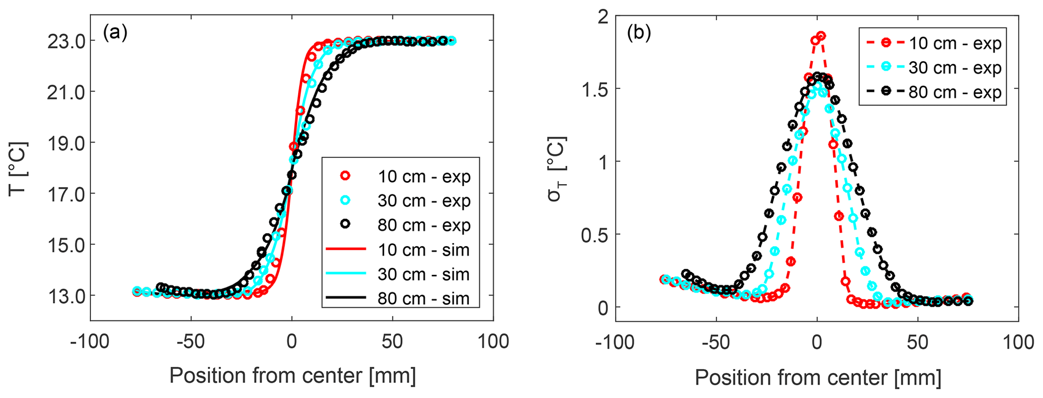
Figure 6(a) Comparison of experimental temperature profiles (circles) with predictions from the simulations (lines) for z1 (in red), z3 (in cyan) and z8 (in black). (b) Experimental results for temperature fluctuations for z1 (in red), z3 (in cyan) and z8 (in black).
Figure 6 shows the time-averaged temperature profiles at three different locations underneath the aerosol inlet. As expected, the turbulent mixing zone widens with increasing distance from the aerosol inlet. There is a slight increase in temperature starting at about −70 mm out of the center caused by heat transfer from the wall as it is in contact with ambient air on the outside which is at a temperature of ∼24 ∘C. The wall on the opposite side consequently does not significantly influence the temperature measurements because here the temperature difference between wall and flow is only ΔT=1 K. However, this wall effect, which will be eliminated in the near future by suitable heat isolation of the measurement section, has a negligible effect on the mixing zone. In addition, the results of the simulations for the mean temperature are included in Fig. 6. The simulations reproduce the measurements in an accurate manner, albeit slightly underestimating the width of the turbulent mixing zone.
The rms temperatures also show the increase in the width of the mixing zone with increasing z. Again, thermal wall effects lead to an increase in the rms temperature towards the wall, however, having a negligible effect on the mixing zone.
After investigating the turbulent transport of heat in dry air ( ∘C), a case with moist air is considered now. The dew-point temperature was set to 12 ∘C in both flow branches (i.e., Td is constant and there is no additional source or sink of water vapor), and the temperature settings corresponded to those of the previous test case (ΔT=10 K and ΔTd=0 K) so that the relative humidities correspond to RHA=50 % and RHB=93 %. The mean dew point in the measurement section was determined with the DPM. To do so, a movable quarter-inch tubing with a vertical inlet was inserted into the measurement section and connected to the DPM. The relative humidity was calculated from the dew-point temperature and the airflow temperature, based on the August–Roche–Magnus empirical formula. In the following, the time-averaged values for temperature, dew-point temperature and relative humidity are presented for the conditions at z3=30 cm recorded along a horizontal profile (see Fig. 7). Additionally, the results of the simulations are depicted. Since the dew-point temperature along the profile is constant, i.e., the partial water vapor pressure is constant, the relative humidity essentially depends only on the temperature. The simulations reproduce the measurements in an accurate manner.
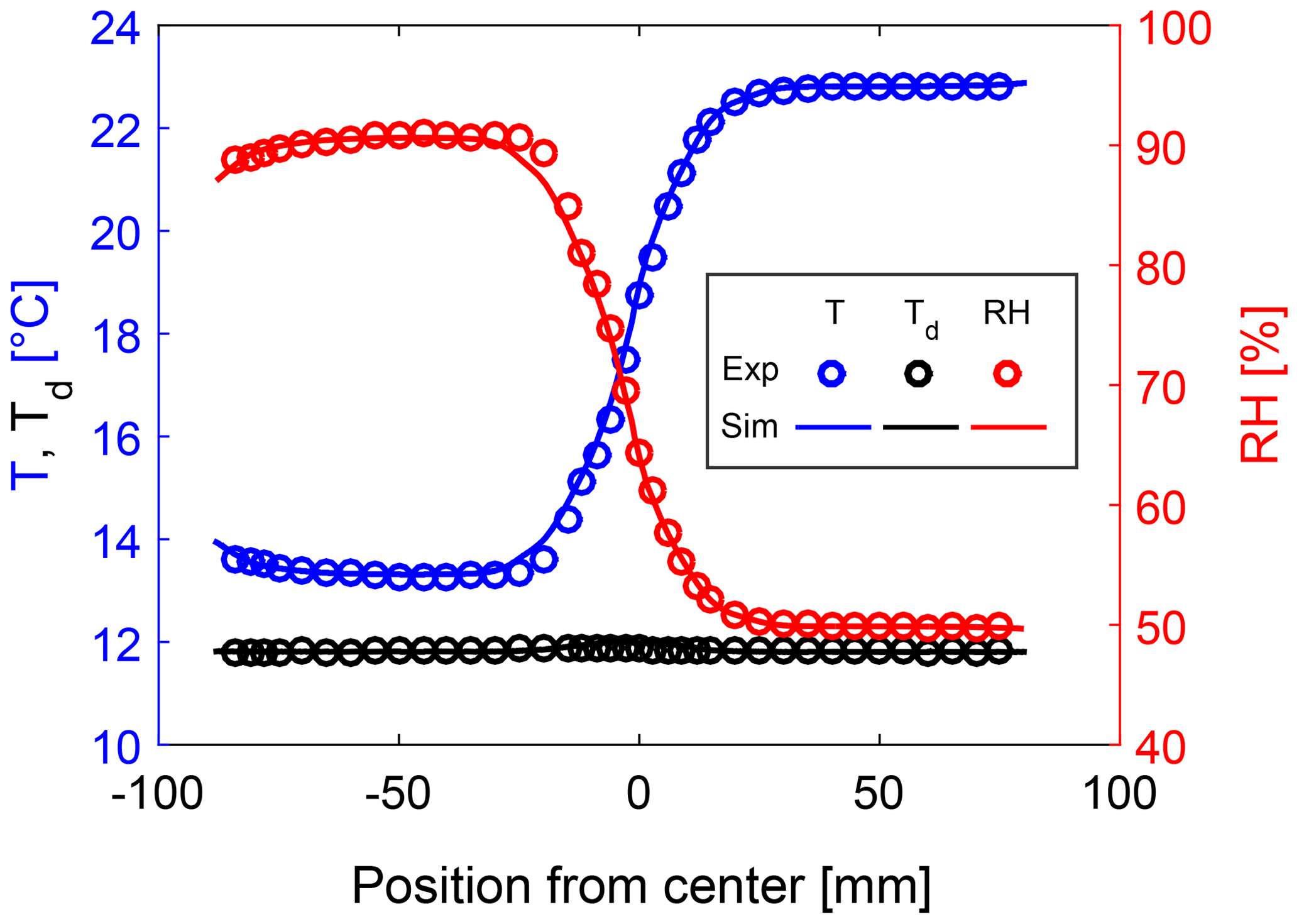
Figure 7Dew-point temperature (black markers), temperature (red markers) and RH profiles (blue markers) including the simulation results, for ΔT=10 K and ΔTd=0 K obtained at z3.
In the previous investigations, we focused on the turbulent transport of heat in dry and moist air. Now, the turbulent transport of mass in addition to heat is studied. To do so, a temperature and a dew-point temperature difference were set between the two particle-free airflows, ΔT=10 K and ΔTd=4 K.
In flow branch A the dew-point temperature was set to ∘C (water vapor mixing ratio g kg−1) and the airflow temperature was set to TA=23 ∘C, resulting in a mean relative humidity of approximately 50 %. Flow branch B featured a dew-point temperature of ∘C (water vapor mixing ratio g kg−1) and an airflow temperature of TB=13 ∘C, leading to approximately 71 % relative humidity. Figure 8 shows the relative humidity profile for z=6, 17 and 30 cm. The turbulent mixing zone expands with increasing distance to the aerosol inlet. The simulations, using the same inlet conditions, reproduce the measurements in an accurate manner, again slightly underestimating the width of the turbulent mixing zone as observed in the previous cases.
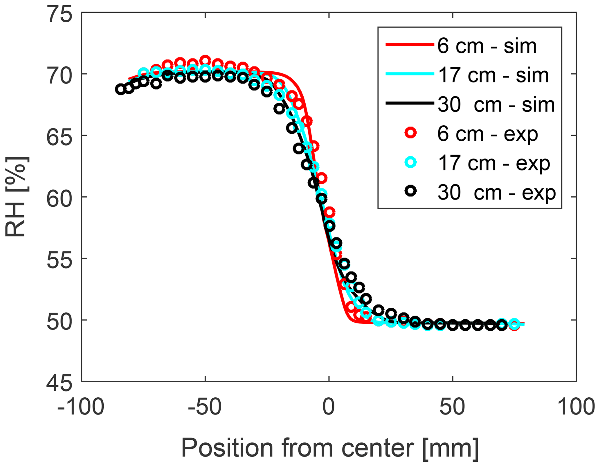
Figure 8RH profiles for ΔT=10 K and ΔTd=4 K based on temperature and dew-point temperature measurements for z=6, 17 and 30 cm including numerical predictions.
Finally, in panel (a) of Fig. 9 we compare the temperature profile (ΔT=10 K) for the different conditions, i.e., dry with ΔTd=0 K, moist with ΔTd=0 K, and moist with ΔTd=4 K, exemplarily for z3. As expected, the temperature profiles shown in Fig. 9a exhibit a very similar behavior; i.e., the influence of the increased amount of water vapor in the airflow as well as the water vapor profile itself (in terms of RH) on the temperature curve are very low. The reason is that still less than 1 % of the total mass is water vapor, which does not significantly influence the fluid properties (e.g., heat capacity). Further, there is no condensation of water vapor which could influence the temperature profile due to latent heat release.
In panel (b) of Fig. 9 the temperature and water vapor mixing are shown for the moist case (ΔTd=4 K). In order to compare both quantities, the normalized water vapor mixing ratio ξn and the normalized temperature θn are depicted. The normalized water vapor mixing ratio is defined as , where qv, 1 and qv, 2 are the lowest and highest water vapor mixing ratios set in the respective flow branch, respectively. The normalized temperature is given through with T1 being the lowest and T2 being the highest temperature set in the respective flow branch. Both curves fall together; i.e, ξn and θn behave similarly as we would expect since turbulent transport processes dominate over laminar diffusion processes in the mixing zone.
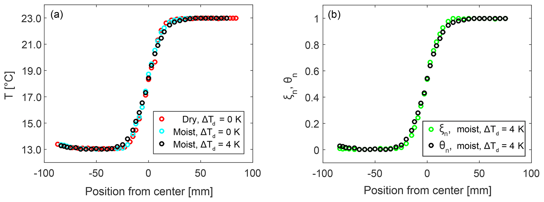
Figure 9(a) Mean temperature profiles for three different cases at z3. (b) Normalized mean temperature and mean mass fraction at z3 for ΔT=10 K and ΔTd=4 K.
In summary, the above-described investigations and results clearly demonstrate the functionality of LACIS-T. The current setup creates sufficiently large regions of homogeneous velocities in the measurement section. Determined dissipation rates are similar to those in atmospheric clouds. The decrease in the turbulent kinetic energy with increasing distance from the turbulence grid is comparable with other wind tunnels. Further, the turbulent mixing behavior of heat in dry air and moist air, as well as the turbulent mixing behavior of water vapor, indicates that the transport of heat and mass in the mixing zone is governed by turbulent processes whereas laminar processes become negligible. Altogether, we observe a well-defined and controllable turbulent mixing process that can be simulated accurately.
The first experiments conducted at LACIS-T deal with the deliquescence, hygroscopic growth and activation of size-selected, monodisperse aerosol particles under turbulent conditions. Sodium chloride particles (NaCl) were used for both experiments. Two different settings have been applied for the studies which will be described accordingly.
5.1 Deliquescence and hygroscopic growth
In the first experiment, the deliquescence and hygroscopic growth behavior of NaCl particles with a dry diameter Dp, dry of 320 nm was investigated. Both particle-free airflows featured the same conditions in terms of flow rate, temperature and dew-point temperature. The temperature and dew-point temperature of the aerosol flow were independently adjusted compared to the two particle-free airflows. The aerosol flow rate was set to enter the measurement section in isokinetic fashion (the inlet concentration was 1000 particles cm−3). The welas 2300 sensor for particle detection was positioned inside the measurement section at z3=30 cm right below the aerosol inlet. The temperature of both particle-free airflows was set to 20 ∘C. The dew-point temperature was varied between 14.4 and 19.8 ∘C, resulting in relative humidities (RHs) in the measurement section between 68 % and 98 %. The particles were introduced into the wind tunnel either dry ( ∘C and T=20 ∘C) or already pre-moistened (Td=19 ∘C and T=20 ∘C), i.e., we investigated the hygroscopic growth of non-deliquesced and deliquesced NaCl particles.
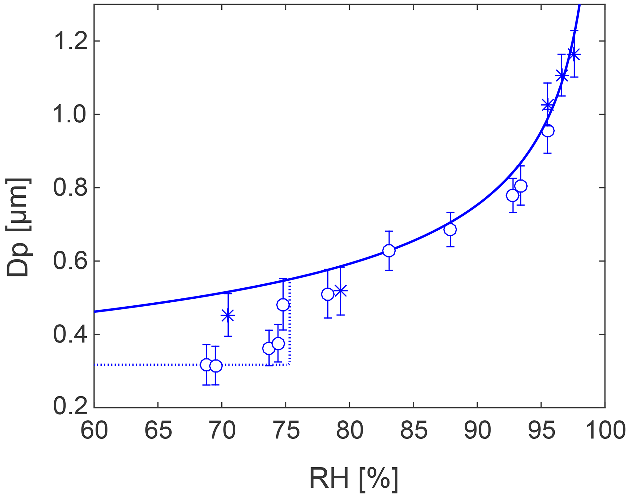
Figure 10Hygroscopic growth of deliquesced (asterisk) and undeliquesced (open circles) NaCl particles with nm at T=20 ∘C with welas 2300. As reference the theoretical Köhler curve for deliquesced particles (solid line) as well as the deliquescence point (dashed line, deliquescence at 75.7 % measured at 25 ∘C by Tang et al., 1977) are shown. We observe deliquescence of NaCl particles at about 75 %.
Figure 10 shows the measured particle diameter versus the relative humidity (obtained through measurements of dew-point and air temperature). The blue solid line represents the corresponding Köhler curve (Pruppacher and Klett, 1997). We observed deliquescence of the NaCl particles at approximately 75 % RH, which compares well to literature data (e.g., 75.7 % measured at 25 ∘C by Tang et al., 1977). Furthermore, deliquescence is observed over a range of RH, which is indicative of an influence of the prevailing turbulent RH fluctuations. Note that the investigations were performed at a total flow rate of 10 000 L min−1, which makes the accuracy of the results even more impressive.
5.2 Droplet activation and growth
In the second experiment, droplet formation on size-selected, monodisperse NaCl particles with Dp, dry of 100, 200, 300 and 400 nm and the subsequent droplet growth were investigated. To do so, a temperature difference of ΔT=16 K was set between the two particle-free airflows. The temperature and dew-point temperature of the airstreams were set to 20 ∘C in branch A and 4 ∘C in branch B, respectively, so that RH=100 % in each airflow. Due to the mixing of both saturated airflows in the measurement section, supersaturation conditions are reached. Based on the simulations (not shown), the mean RH was at approximately 101.5 %.
For each injected Dp, dry, the particle concentration was set to 1000 cm−3. The welas 2300 sensor was positioned at the center position inside the measurement section at z4=40 cm or z8=80 cm, in order to determine the prevailing droplet size distributions.
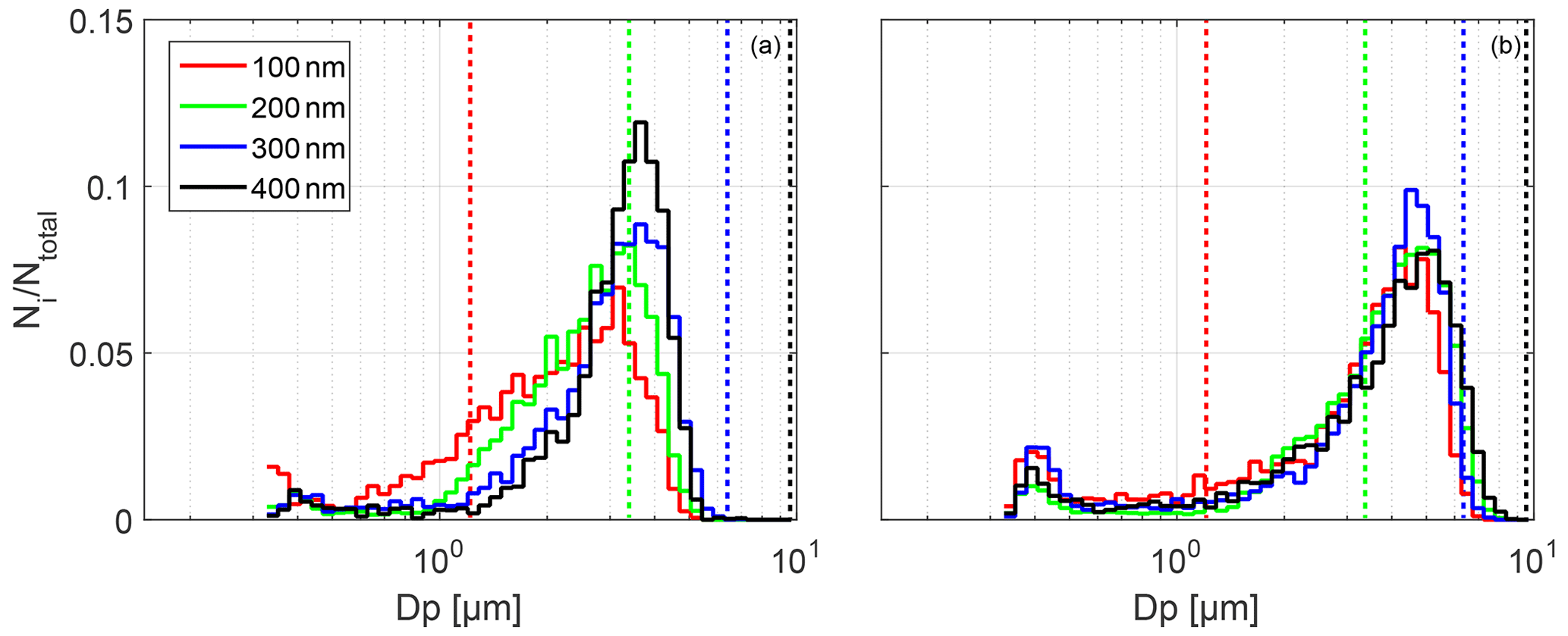
Figure 11Droplet formation and growth of differently size-selected, monodisperse NaCl particles ( nm) for ΔT=16 K measured at two different positions below the aerosol inlet (a: z4=40 cm, b: z8=80 cm). The dotted lines represent the critical diameters Dp, crit for particle activation which are 1.2, 3.4, 6.3 and 9.7 µm for , 200, 300 and 400 nm, respectively.
The determined size distributions at the two positions are shown in Fig. 11. In both figures, the normalized droplet number vs. the particle diameter is displayed. The following observations can be made: (a) for each Dp, dry the formed droplets grow with increasing distance to the aerosol inlet, (b) all the size distributions nearly fall together at z8 (see Fig. 11b), (c) the size distributions are negatively skewed and (d) we also observe a significant number of particles close to Dp=300 nm, which is approximately the welas 2300 detection limit.
To start with the interpretation of these observations, we included the critical diameters Dp, crit for particle activation which are 1.2, 3.4, 6.3 and 9.7 µm (dotted lines in Fig. 11) for , 200, 300 and 400 nm, respectively. For all dry particle sizes investigated, the supersaturation reached inside the measurement section is high enough to activate these particles to cloud droplets. However, only the grown droplets which originate from the nm and nm particles are almost all or mostly activated at z8 while the ones formed on the nm and nm particles are mostly not. The reason for this observation is the kinetic limitation of droplet growth. The time the particles are exposed to a certain level of supersaturation must be long enough to reach the respective critical diameter (Chuang et al., 1997; Nenes et al., 2001). For the and 400 nm particles and the prevailing supersaturation, this time is on the order of several tens of seconds. However, the time to reach z8 is about 0.5 s, which is too short for these particles to reach their respective Dp, crit. Naturally, it also limits the further growth of the droplets which formed on the nm and nm particles, as for the diffusional growth it is irrelevant whether the droplets are activated or not as long as the supersaturation is above the critical value, which depends on the dry particle size. In conclusion, under the prevailing conditions and the sole observation of the grown droplet distributions, it is not possible to distinguish between the activated and nonactivated droplet distributions or to determine which distribution represents the activated and which the not-activated state. In other words, droplet growth is kinetically limited regardless of whether the droplets are in the hygroscopic or dynamic growth regime. Further, the dry particle size is of minor importance for the observed droplet distributions, especially with increasing residence time.
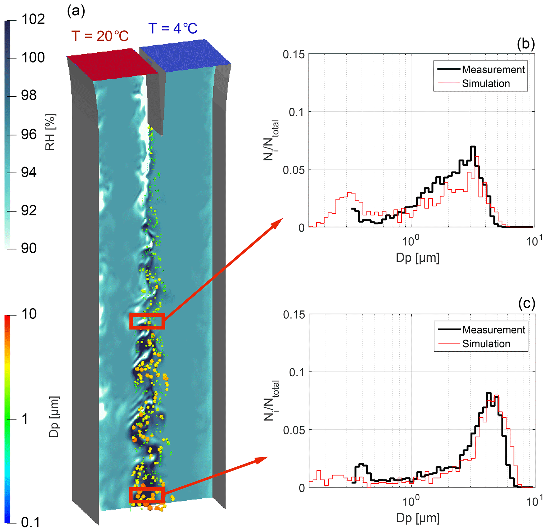
Figure 12Snapshot of particle simulation with fluctuating relative humidity field in the background and particles colored and sized (not to scale) according to their diameter. (b, c) Droplet formation and growth of monodisperse NaCl particles ( nm) for ΔT=16 K measured at two different positions below the aerosol inlet (b: z4, c: z8) for measurements (black line) and simulations (red line).
In order to interpret the negative skewness of the distributions as well as the significant number of particles close to Dp=300 nm, we consider the LES results which are shown in Fig. 12. In panel (a), a snapshot of the instantaneous saturation field in the symmetry plane as well as the respective particle diameters grown on nm NaCl particles along the vertical axis are shown. For z4 and z8, droplet size distributions are extracted from the simulations and displayed together with the measured size distributions in Fig. 12b, c. From the simulations, the magnitude of the RH fluctuations in terms of a standard deviation can be determined to be %.
First of all, the simulations reproduce the measurements in an accurate manner. At z4, the simulated droplet distribution is of bimodal shape where the left shoulder of the first mode was not detected by the welas 2300 due to its detection limit. Further the negative skewness can be observed in both sub-figures. From the simulation of individual particle tracks (not shown) it can be concluded that the small particles () are hygroscopically grown particles that did not experience supersaturated conditions but also droplets that deactivated because they experienced subsaturated conditions in the fluctuating saturation field. In general, these turbulent fluctuations in RH broaden the droplet size distribution towards smaller diameters due to evaporating droplets or less-grown droplets in the left tail of the droplet size distribution. In other words, the negative skewness of the obtained droplet size distributions is indicative of turbulence-influenced droplet formation and growth or evaporation. The particle size plays a minor role here.
Finally, as kind of a benchmark, we want to evaluate what the droplet size distribution would look like without turbulence affecting droplet formation and growth. Therefore, utilizing the above-described numerical model, two additional cases have been investigated, (a) a case without grid-induced turbulence (i.e., the grid was removed from the numerical simulation) and (b) an idealized case based on time-averaged flow fields without turbulent fluctuations. In these simulations the formation and growth of NaCl particles, with nm for the temperature difference of ΔT=16 K, were considered. The simulation results are shown in Fig. 13 for z8=80 cm together with measurement results, for which the turbulence grid remains included as shown in Fig. 12.
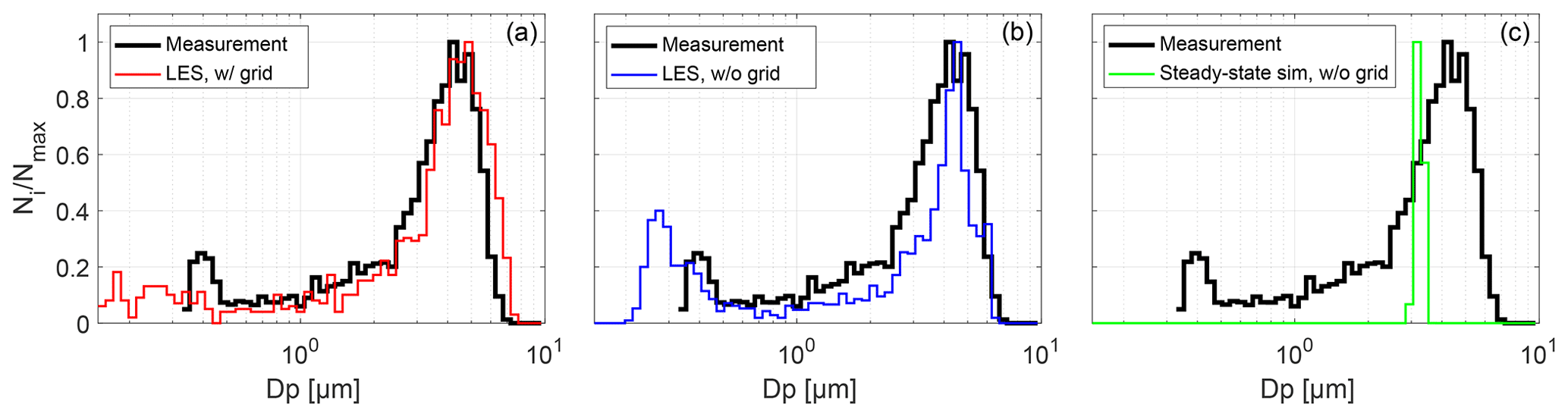
Figure 13Comparison between different model calculations for the particle formation and growth on NaCl particles with nm at z8 for ΔT=16 K. (a) LES with turbulence grid (as shown in (c) of Fig. 12). (b) LES but without turbulence grid. (c) Simulation with averaged fields used as frozen flow fields, and transient particle calculation. In all plots, the measurement results, for which the turbulence grid is included (as shown in (c) of Fig. 12), are shown for reference.
It turns out that the removal of the turbulence grid does not lead to laminar conditions. We still observe inherent turbulent conditions due to wall effects and the high Reynolds number (order of 104) for the set velocity. But the turbulence intensity and therefore the strength of turbulent fluctuations are decreased. The power spectra obtained for the configuration without a grid further suggest that the turbulence is anisotropic in this case (not shown). As a consequence, we still obtain a broad droplet size distribution (see panel (b) in Fig. 13) which is however narrower compared to the measurement–simulation with the turbulence grid. We also observe a significant number of particles close to Dp=300 nm.
Laminar conditions, which would lead to a very narrow droplet size distribution (see panel (c) in Fig. 13), can only be simulated if averaged fields are used as frozen flow fields in the simulations, which is not realizable in the real measurement. In other words, measurements without turbulence are not executable inside LACIS-T and the flow regime is best controlled in the presence of the turbulence grid. Furthermore, these simulations clearly indicate the distinct influences of turbulence on the droplet size distributions and, consequently, on the formation and growth of droplets inside LACIS-T.
We have developed the turbulent moist-air wind tunnel LACIS-T, specifically aiming at a better understanding of aerosol–cloud–turbulence interactions. The advantage of LACIS-T in particular and laboratory experiments in general is that specific, atmospherically relevant processes can be studied under well-controlled and repeatable initial and boundary conditions, whereas in field experiments, there often is significant uncertainty in the measurements themselves, in the prevailing boundary conditions and in the statistical stationarity of conditions (Chang et al., 2016). Furthermore, laboratory experiments can provide scenarios for which physical theory and models can be directly compared to an experiment, with known initial and boundary conditions (Stratmann et al., 2009). Therefore, laboratory experiments, in which the turbulence and thermodynamic conditions are reliably reproducible and long-term averaging of measurements under statistically stationary conditions can be achieved, are invaluable for increasing our quantitative understanding concerning atmospheric cloud processes.
The investigations described here show that LACIS-T is suitable for studying the influence of turbulent temperature and water vapor fluctuations on cloud microphysical processes. We observed deliquescence to take place over a range of mean RH, which is indicative of a prevailing influence of turbulent RH fluctuations. We further obtained indications of the influence of turbulent supersaturation fluctuations on the droplet activation. Concerning the latter, our results also suggest that kinetic effects and/or limitations may be important in inhibiting droplet activation in a turbulent environment. On the other hand, turbulence can also lead to the occurrence of locally high supersaturations, which, together with the highly nonlinear Köhler and condensational growth equations, might increase the number of activated droplets. Altogether, turbulent fluctuations affect the droplet size distribution. Our first results are very promising in terms of the ability to capture the observed processes with the LES, as well as the ability to see clear indications of the effect of turbulence on droplet activation and growth. These results will be verified and quantified in more detail in the near future. In that sense we will also focus on the relative roles of turbulence vs. aerosol particle physical and chemical properties (particle size, number and composition).
We further aim at gaining fundamental and quantitative understanding of the influences of entrainment and detrainment processes on the microphysical properties of clouds as well as the influence of turbulence on heterogeneous ice nucleation in the near future. LACIS-T is also part of the EU-funded (HORIZON 2020) infrastructure project EUROCHAMP-2020 which is planned to be embedded into ACTRIS (Aerosol, Cloud and Trace Gases Research Infrastructure). In the scope of the infrastructure projects, LACIS-T is being made available to other scientists from the atmospheric science community to address interdisciplinary problems as well as to use the wind tunnel for scientific instrument testing and calibration.
In summary, results from LACIS-T investigations will have the potential to help interpret and corroborate the results from related in situ measurements in clouds (e.g., Ditas et al., 2012) and therefore enhance our understanding of the interactions between cloud microphysics and turbulence and consequently cloud processes in general.
The experimental data are available via the EUROCHAMP-2020 (https://data.eurochamp.org/data-access/chamber-experiments/, last access: 9 April 2020) data center as well as upon request to the contact author. For numerical data please contact Silvio Schmalfuß (schmalfuss@tropos.de) or Dennis Niedermeier.
DN and SiS (Sect. 3) wrote the manuscript with contributions from all co-authors. LACIS-T measurements and data evaluation were performed by DN, DB, JV and SiS. Numerical simulations were performed by SiS with contributions from DN, JV and FS. All authors discussed the experimental and numerical results. FS initiated and conducted the conceptualization, planning and buildup of LACIS-T with significant contributions from JV, JS and RAS.
The authors declare that they have no conflict of interest.
This article is part of the special issue “Simulation chambers as tools in atmospheric research (AMT/ACP/GMD inter-journal SI)”. It is not associated with a conference.
LACIS-T was constructed in the framework of the Leibniz SAW project “Leipzig Aerosol Cloud Turbulence Tunnel” (no. SAW-2013-IfT-2). This project/work has also received funding from the European Commission, H2020 Research Infrastructures (EUROCHAMP-2020 (grant no. 730997)). Dennis Niedermeier acknowledges support from the Alexander von Humboldt Foundation.
This research has been supported by the Leibniz Association (project no. SAW-2013-IfT-2) and by the European Commission, H2020 Research Infrastructures (EUROCHAMP-2020 (grant no. 730997)). Dennis Niedermeier obtained financial support from the Alexander von Humboldt Foundation.
The publication of this article was funded by the
Open Access Fund of the Leibniz Association.
This paper was edited by Jonathan Abbatt and reviewed by two anonymous referees.
Augustin, S., Wex, H., Niedermeier, D., Pummer, B., Grothe, H., Hartmann, S., Tomsche, L., Clauss, T., Voigtländer, J., Ignatius, K., and Stratmann, F.: Immersion freezing of birch pollen washing water, Atmos. Chem. Phys., 13, 10989–11003, https://doi.org/10.5194/acp-13-10989-2013, 2013. a
Augustin-Bauditz, S., Wex, H., Kanter, S., Ebert, M., Niedermeier, D., Stolz, F., Prager, A., and Stratmann, F.: The immersion mode ice nucleation behavior of mineral dusts: A comparison of different pure and surface modified dusts, Geophys. Res. Lett., 41, 7375–7382, https://doi.org/10.1002/2014GL061317, 2014. a
Bodenschatz, E., Malinowski, S. P., Shaw, R. A., and Stratmann, F.: Can we understand clouds without turbulence?, Science, 327, 970–971, https://doi.org/10.1126/science.1185138, 2010. a, b
Bohren, C. F. and Albrecht, B. A.: Atmospheric thermodynamics, Oxford University Press, New York, 1998. a
Chai, X. and Mahesh, K.: Dynamic-equation model for large-eddy simulation of compressible flows, J. Fluid Mech., 699, 385–413, https://doi.org/10.1017/jfm.2012.115, 2012. a
Chandrakar, K. K., Cantrell, W., Chang, K., Ciochetto, D., Niedermeier, D., Ovchinnikov, M., Shaw, R. A., and Yang, F.: Aerosol indirect effect from turbulence-induced broadening of cloud-droplet size distributions, P. Natl. Acad. Sci. USA, 113, 14243–14248, https://doi.org/10.1073/pnas.1612686113, 2016. a, b
Chandrakar, K. K., Saito, I., Yang, F., Cantrell, W., Gotoh, T., and Shaw, R. A.: Droplet size distributions in turbulent clouds: experimental evaluation of theoretical distributions, Q. J. Roy. Meteorol. Soc., 146, 483–504, https://doi.org/10.1002/qj.3692, 2020. a
Chang, K., Bench, J., Brege, M., Cantrell, W., Chandrakar, K., Ciochetto, D., Mazzoleni, C., Mazzoleni, L., Niedermeier, D., and Shaw, R.: A laboratory facility to study gas–aerosol–cloud interactions in a turbulent environment: The Π chamber, B. Am. Meteorol. Soc., 97, 2343–2358, https://doi.org/10.1175/BAMS-D-15-00203.1, 2016. a, b, c, d, e
Chuang, P., Charlson, R. J., and Seinfeld, J.: Kinetic limitations on droplet formation in clouds, Nature, 390, 594–596, https://doi.org/10.1038/37576, 1997. a
Cziczo, D. J., Ladino, L., Boose, Y., Kanji, Z. A., Kupiszewski, P., Lance, S., Mertes, S., and Wex, H.: Measurements of ice nucleating particles and ice residuals, Meteor. Mon., 58, 8.1–8.13, https://doi.org/10.1175/AMSMONOGRAPHS-D-16-0008.1, 2017. a
Ditas, F., Shaw, R. A., Siebert, H., Simmel, M., Wehner, B., and Wiedensohler, A.: Aerosols-cloud microphysics-thermodynamics-turbulence: evaluating supersaturation in a marine stratocumulus cloud, Atmos. Chem. Phys., 12, 2459–2468, https://doi.org/10.5194/acp-12-2459-2012, 2012. a
EUROCHAMP-2020: https://data.eurochamp.org/data-access/chamber-experiments/, last access: 9 April 2020.
Fuchs, N. A. and Sutugin, A. G.: Highly Dispersed Aerosols, 105 pp., translated from Russian by Isr. Program for Sci. Transl., Ann. Arbor Sci., Ann Arbor, MI, USA, 1970. a
Grawe, S., Augustin-Bauditz, S., Hartmann, S., Hellner, L., Pettersson, J. B. C., Prager, A., Stratmann, F., and Wex, H.: The immersion freezing behavior of ash particles from wood and brown coal burning, Atmos. Chem. Phys., 16, 13911–13928, https://doi.org/10.5194/acp-16-13911-2016, 2016. a
Grawe, S., Augustin-Bauditz, S., Clemen, H.-C., Ebert, M., Eriksen Hammer, S., Lubitz, J., Reicher, N., Rudich, Y., Schneider, J., Staacke, R., Stratmann, F., Welti, A., and Wex, H.: Coal fly ash: linking immersion freezing behavior and physicochemical particle properties, Atmos. Chem. Phys., 18, 13903–13923, https://doi.org/10.5194/acp-18-13903-2018, 2018. a
Hartmann, S., Niedermeier, D., Voigtländer, J., Clauss, T., Shaw, R. A., Wex, H., Kiselev, A., and Stratmann, F.: Homogeneous and heterogeneous ice nucleation at LACIS: operating principle and theoretical studies, Atmos. Chem. Phys., 11, 1753–1767, https://doi.org/10.5194/acp-11-1753-2011, 2011. a
Hartmann, S., Augustin, S., Clauss, T., Wex, H., Šantl-Temkiv, T., Voigtländer, J., Niedermeier, D., and Stratmann, F.: Immersion freezing of ice nucleation active protein complexes, Atmos. Chem. Phys., 13, 5751–5766, https://doi.org/10.5194/acp-13-5751-2013, 2013. a
Hartmann, S., Wex, H., Clauss, T., Augustin-Bauditz, S., Niedermeier, D., Rösch, M., and Stratmann, F.: Immersion freezing of kaolinite: Scaling with particle surface area, J. Atmos. Sci., 73, 263–278, https://doi.org/10.1175/JAS-D-15-0057.1, 2016. a
Henning, S., Wex, H., Hennig, T., Kiselev, A., Snider, J., Rose, D., Dusek, U., Frank, G., Pöschl, U., Kristensson, A., Bilde, M., Tillmann, R., Kiendler-Scharr, A., Mentel, T. F., Walter, S., Schneider, J., Wennrich, C., and Stratmann, F.: Soluble mass, hygroscopic growth, and droplet activation of coated soot particles during LACIS Experiment in November (LExNo), J. Geophys. Res., 115, D11206, https://doi.org/10.1029/2009JD012626, 2010. a
Hobbs, P. V.: Research on clouds and precipitation: Past, present and future, Part II, B. Am. Meteorol. Soc., 72, 184–191, https://doi.org/10.1175/1520-0477(1991)072<0184:ROCAPP>2.0.CO;2, 1991. a
Knutson, E. and Whitby, K.: Aerosol classification by electric mobility: apparatus, theory, and applications, J. Aerosol Sci., 6, 443–451, https://doi.org/10.1016/0021-8502(75)90060-9, 1975. a
Kreidenweis, S. M., Petters, M., and Lohmann, U.: 100 years of progress in cloud physics, aerosols, and aerosol chemistry research, Meteor. Mon., 59, 11.1–11.72, https://doi.org/10.1175/AMSMONOGRAPHS-D-18-0024.1, 2019. a, b, c
Kumar, B., Götzfried, P., Suresh, N., Schumacher, J., and Shaw, R. A.: Scale Dependence of Cloud Microphysical Response to Turbulent Entrainment and Mixing, J. Adv. Model. Earth Sy., 10, 2777–2785, https://doi.org/10.1029/2018MS001487, 2018. a, b
Lamb, D. and Verlinde, J.: Physics and chemistry of clouds, Cambridge University Press, Cambridge, UK, 2011. a
Lavoie, P., Djenidi, L., and Antonia, R. A.: Effects of initial conditions in decaying turbulence generated by passive grids, J. Fluid Mech., 585, 395–420, https://doi.org/10.1017/S0022112007006763, 2007. a
List, R., Hallett, J., Warner, J., and Reinking, R.: The Future of Laboratory Research and Facilities for Cloud Physics and Cloud Chemistry: Report on a Technical Workshop Held in Boulder, Colorado, 20–22 March 1985, B. Am. Meteorol. Soc., 67, 1389–1397, https://doi.org/10.1175/1520-0477-67.11.1389, 1986. a
Malinowski, S. P., Andrejczuk, M., Grabowski, W. W., Korczyk, P., Kowalewski, T. A., and Smolarkiewicz, P. K.: Laboratory and modeling studies of cloud–clear air interfacial mixing: anisotropy of small-scale turbulence due to evaporative cooling, New J. Phys., 10, 075020, https://doi.org/10.1088/1367-2630/10/7/075020, 2008. a
Mason, B. J. and Ludlam, F. H.: The microphysics of clouds, Rep. Prog. Phys., 14, 147–195, https://doi.org/10.1088/0034-4885/14/1/306, 1951. a
McGraw, R. and Liu, Y.: Brownian drift-diffusion model for evolution of droplet size distributions in turbulent clouds, Geophys. Res. Lett., 33, L03802, https://doi.org/10.1029/2005GL023545, 2006. a
Mei, R.: An approximate expression for the shear lift force on a spherical particle at finite Reynolds number, Int. J. Multiphas. Flow, 18, 145–147, https://doi.org/10.1016/0301-9322(92)90012-6, 1992. a
Nenes, A., Ghan, S., Abdul-Razzak, H., Chuang, P. Y., and Seinfeld, J. H.: Kinetic limitations on cloud droplet formation and impact on cloud albedo, Tellus B, 53, 133–149, https://doi.org/10.3402/tellusb.v53i2.16569, 2001. a
Niedermeier, D., Wex, H., Voigtländer, J., Stratmann, F., Brüggemann, E., Kiselev, A., Henk, H., and Heintzenberg, J.: LACIS-measurements and parameterization of sea-salt particle hygroscopic growth and activation, Atmos. Chem. Phys., 8, 579–590, https://doi.org/10.5194/acp-8-579-2008, 2008. a
Niedermeier, D., Hartmann, S., Shaw, R. A., Covert, D., Mentel, T. F., Schneider, J., Poulain, L., Reitz, P., Spindler, C., Clauss, T., Kiselev, A., Hallbauer, E., Wex, H., Mildenberger, K., and Stratmann, F.: Heterogeneous freezing of droplets with immersed mineral dust particles – measurements and parameterization, Atmos. Chem. Phys., 10, 3601–3614, https://doi.org/10.5194/acp-10-3601-2010, 2010. a
Petters, M. D., Wex, H., Carrico, C. M., Hallbauer, E., Massling, A., McMeeking, G. R., Poulain, L., Wu, Z., Kreidenweis, S. M., and Stratmann, F.: Towards closing the gap between hygroscopic growth and activation for secondary organic aerosol – Part 2: Theoretical approaches, Atmos. Chem. Phys., 9, 3999–4009, https://doi.org/10.5194/acp-9-3999-2009, 2009. a
Pruppacher, H. R. and Klett, J. D.: Microphysics of Clouds and Precipitation, Kluwer Academic Publishers, Dordrecht, The Netherlands, 1997. a
Quaas, J., Bony, S., Collins, W. D., Donner, L., Illingworth, A., Jones, A., Lohmann, U., Satoh, M., Schwartz, S. E., Tao, W. K., and Wood, R.: Current understanding and quantification of clouds in the changing climate system and strategies for reducing critical uncertainties, in: Clouds in the perturbed climate system: Their Relationship to Energy Balance, Atmospheric Dynamics, and Precipitation, edited by: Heintzenberg, J. and Charlson, R. J., MIT Press, Cambridge, MA, USA, 557–573, 2009. a
Randers-Pehrson, N.: Pioneer wind tunnels, Smithsonian Miscellaneous Collections, 93, 1–20, 1935. a
Saito, I., Gotoh, T., and Watanabe, T.: Broadening of cloud droplet size distributions by condensation in turbulence, J. Meteorol. Soc. Jpn., 97, 867–891, https://doi.org/10.2151/jmsj.2019-049, 2019. a
Schiller, L. and Naumann, A.: Fundamental calculations in gravitational processing, Z. Ver. Dtsch. Ing., 77, 318–320, 1933. a
Schumacher, J., Sreenivasan, K. R., and Yakhot, V.: Asymptotic exponents from low-Reynolds-number flows, New J. Phys., 9, 89, https://doi.org/10.1088/1367-2630/9/4/089, 2007. a
Seinfeld, J. H., Bretherton, C., Carslaw, K. S., Coe, H., DeMott, P. J., Dunlea, E. J., Feingold, G., Ghan, S., Guenther, A. B., Kahn, R., Kraucunas, I., Kreidenweis, S. M., Molina, M. J., Nenes, A., Penner, J. E., Prather, K. A., Ramanathan, V., Ramaswamy, V., Rasch, P. J., Ravishankara, A. R., Rosenfeld, D., Stephens, G., and Wood, R.: Improving our fundamental understanding of the role of aerosol-cloud interactions in the climate system, P. Natl. Acad. Sci. USA, 113, 5781–5790, https://doi.org/10.1073/pnas.1514043113, 2016. a
Shaw, R. A.: Particle-turbulence interactions in atmospheric clouds, Annu. Rev. Fluid Mech., 35, 183–227, https://doi.org/10.1146/annurev.fluid.35.101101.161125, 2003. a
Shi, X., Hagen, H. L., Chow, F. K., Bryan, G. H., and Street, R. L.: Large-eddy simulation of the stratocumulus-capped boundary layer with explicit filtering and reconstruction turbulence modeling, J. Atmos. Sci., 75, 611–637, https://doi.org/10.1175/JAS-D-17-0162.1, 2018. a
Siebert, H. and Shaw, R. A.: Supersaturation fluctuations during the early stage of cumulus formation, J. Atmos. Sci., 74, 975–988, https://doi.org/10.1175/JAS-D-16-0115.1, 2017. a
Siebert, H., Franke, H., Lehmann, K., Maser, R., Saw, E. W., Schell, D., Shaw, R. A., and Wendisch, M.: Probing finescale dynamics and microphysics of clouds with helicopter-borne measurements, B. Am. Meteorol. Soc., 87, 1727–1738, https://doi.org/10.1175/BAMS-87-12-1727, 2006. a
Siebert, H., Gerashchenko, S., Gylfason, A., Lehmann, K., Collins, L., Shaw, R., and Warhaft, Z.: Towards understanding the role of turbulence on droplets in clouds: in situ and laboratory measurements, Atmos. Res., 97, 426–437, https://doi.org/10.1016/j.atmosres.2010.05.007, 2010. a
Stevens, B., Moeng, C.-H., Ackerman, A. S., Bretherton, C. S., Chlond, A., de Roode, S., Edwards, J., Golaz, J.-C., Jiang, H., Khairoutdinov, M., Kirkpatrick, M. P., Lewellen, D. C., Lockl, A., Müller, F., Stevens, D. E., Whelan, E., and Zhu, P.: Evaluation of large-eddy simulations via observations of nocturnal marine stratocumulus, Mon. Weather Rev., 133, 1443–1462, https://doi.org/10.1175/MWR2930.1, 2005. a
Stokes, G. G.: On the effect of the internal friction of fluids on the motion of pendulums, in: Transactions of the Cambridge Philosophical Society, Pitt Press Cambridge, 9, 8–106, 1851. a
Stratmann, F., Kiselev, A., Wurzler, S., Wendisch, M., Heintzenberg, J., Charlson, R., Diehl, K., Wex, H., and Schmidt, S.: Laboratory studies and numerical simulations of cloud droplet formation under realistic supersaturation conditions, J. Atmos. Ocean. Tech., 21, 876–887, https://doi.org/10.1175/1520-0426(2004)021<0876:LSANSO>2.0.CO;2, 2004. a
Stratmann, F., Möhler, O., Shaw, R. A., and Wex, H.: Laboratory cloud simulation: Capabilities and future directions, in: Clouds in the Perturbed Climate System: Their Relationship to Energy Balance, Atmospheric Dynamics, and Precipitation, edited by: Heintzenberg, J. and Charlson, R. J., MIT Press, Cambridge, MA, USA, 149–172, 2009. a, b, c
Stratmann, F., Bilde, M., Dusek, U., Frank, G. P., Hennig, T., Henning, S., Kiendler-Scharr, A., Kiselev, A., Kristensson, A., Lieberwirth, I., Mentel, T. F., Pöschl, U., Rose, D., Schneider, J., Snider, J. R., Tillmann, R., Walter, S., and Wex, H.: Examination of laboratory-generated coated soot particles: An overview of the LACIS Experiment in November (LExNo) campaign, J. Geophys. Res., 115, D11203, https://doi.org/10.1029/2009JD012628, 2010. a
Tang, I., Munkelwitz, H., and Davis, J.: Aerosol growth studies-II. Preparation and growth measurements of monodisperse salt aerosols, J. Aerosol Sci., 8, 149–159, https://doi.org/10.1016/0021-8502(77)90002-7, 1977. a, b
Voigtländer, J., Stratmann, F., Niedermeier, D., Wex, H., and Kiselev A.: Mass accommodation coefficient of water: A combined computational fluid dynamics and experimental data analysis, J. Geophys. Res., 112, D20208, https://doi.org/10.1029/2007JD008604, 2007. a
Wang, L.-P. and Grabowski, W. W.: The role of air turbulence in warm rain initiation, Atmos. Sci. Lett., 10, 1–8, https://doi.org/10.1002/asl.210, 2009. a
Wex, H., Kiselev, A., Stratmann, F., Zoboki, J., and Brechtel, F.: Measured and modeled equilibrium sizes of NaCl and (NH4)2SO4 particles at relative humidities up to 99.1 %, J. Geophys. Res., 110, D21212, https://doi.org/10.1029/2004JD005507, 2005. a
Wex, H., Hennig, T., Salma, I., Ocskay, R., Kiselev, A., Henning, S., Massling, A., Wiedensohler, A., and Stratmann, F.: Hygroscopic growth and measured and modeled critical super-saturations of an atmospheric HULIS sample, Geophys. Res. Lett., 34, L02818, https://doi.org/10.1029/2006GL028260, 2007. a
Wex, H., Petters, M. D., Carrico, C. M., Hallbauer, E., Massling, A., McMeeking, G. R., Poulain, L., Wu, Z., Kreidenweis, S. M., and Stratmann, F.: Towards closing the gap between hygroscopic growth and activation for secondary organic aerosol: Part 1 – Evidence from measurements, Atmos. Chem. Phys., 9, 3987–3997, https://doi.org/10.5194/acp-9-3987-2009, 2009. a
Wilck, M.: Modal Modelling of Multicomponent Aerosols, VWF Verlag für Forschung GmbH, Berlin, 1998. a
Wyngaard, J. C.: Turbulence in the Atmosphere, Cambridge University Press, Cambridge, UK, 2010. a
Ziese, M., Wex, H., Nilsson, E., Salma, I., Ocskay, R., Hennig, T., Massling, A., and Stratmann, F.: Hygroscopic growth and activation of HULIS particles: experimental data and a new iterative parameterization scheme for complex aerosol particles, Atmos. Chem. Phys., 8, 1855–1866, https://doi.org/10.5194/acp-8-1855-2008, 2008. a
Note that we do not observe a significant difference between dry and moist conditions or for isothermal and non-isothermal conditions.
- Abstract
- Introduction
- Technical description of LACIS-T
- Numerical simulations
- Characterization of the flow and thermodynamic properties
- First experimental results on particle deliquescence–hygroscopic growth and droplet activation–growth
- Summary and outlook
- Data availability
- Author contributions
- Competing interests
- Special issue statement
- Acknowledgements
- Financial support
- Review statement
- References