the Creative Commons Attribution 4.0 License.
the Creative Commons Attribution 4.0 License.
 | 07 May 2020
Mapping ice formation to mineral-surface topography using a micro mixing chamber with video and atomic-force microscopy
Raymond W. Friddle
Konrad Thürmer
We developed a method for examining ice formation on solid substrates exposed to cloud-like atmospheres. Our experimental approach couples video-rate optical microscopy of ice formation with high-resolution atomic-force microscopy (AFM) of the initial mineral surface. We demonstrate how colocating stitched AFM images with video microscopy can be used to relate the likelihood of ice formation to nanoscale properties of a mineral substrate, e.g., the abundance of surface steps of a certain height. We also discuss the potential of this setup for future iterative investigations of the properties of ice nucleation sites on materials.
- Article
(6745 KB) - Full-text XML
- BibTeX
- EndNote


Ice formation1 in the atmosphere initiates most precipitation and strongly affects Earth's radiation balance (Pruppacher and Klett, 1997; Rogers and Yau, 1989; Lohmann and Feichter, 2005; DeMott et al., 2010; Lau and Wu, 2003). Ice emerges via various microscopic processes (Kanji et al., 2017; Pruppacher and Klett, 1997; Rogers and Yau, 1989; Vali et al., 2015); some require the presence of a foreign material (heterogenous nucleation), while others proceed unaided by any foreign substance (homogeneous nucleation). For ice nucleation to occur above ∘C, a suitable ice-nucleating particle (INP) must provide a surface onto which an ice nucleus can grow to a critical size without being impeded by an insurmountable activation barrier. Most ice nucleation events occur at atmospheric conditions where the critical nucleus size ranges from ∼1 to ∼50 nm (Pruppacher and Klett, 1997). Uncovering the mechanisms involved in these events thus requires nanometer-resolution techniques.
While structure, morphology, particle size, and the presence of defects or functional groups have been found to determine the ice-nucleating ability of aerosols, the role of these properties and how they interact remain poorly understood (Coluzza et al., 2017; DeMott et al., 2011; Kanji et al., 2017; Koop and Mahowald, 2013; Pruppacher and Klett, 1997; Welti et al., 2014). Nevertheless, recent ice nucleation parameterizations, relating the concentration of INPs to the concentration of aerosol particles above a threshold size (DeMott et al., 2010), the aerosols' chemical composition (Vergara-Temprado et al., 2018), or water and substrate contact angles (Wang et al., 2014) and averaged field measurements, have succeeded in improving the accuracy of global climate models. However, as is true for extrapolations in general, such models are expected to be less accurate when applied to conditions outside the range of measured values used to fine-tune these models, e.g., to predict a changing environment due to global warming or to predict the behavior under extreme regional conditions, say, in plumes of dust or contamination. Developing a capability to predict ice formation in these uncharted atmospheric conditions with some confidence will require a quantitative understanding of the underlying mechanisms. Since macroscopic measurements of nucleation rates often cannot distinguish clearly between nucleation mechanisms (Kanji et al., 2017; Marcolli, 2014; Pruppacher and Klett, 1997; Welti et al., 2014; Vali et al., 2015), innovative microscopy aimed at uncovering the local structural and chemical properties of ice nucleation sites is needed.
The technical requirements to adequately resolve ice nucleation in time and space are indeed demanding. The imaging system must operate in humid environments, at sub-0 ∘C temperatures; be nondestructive; and offer a spatial resolution on the order of nanometers. Finally, to locate the ice nucleation site to within nanometers, the frame rate must be fast enough to capture the earliest emergence of the crystalline phase. As a point of reference, our data at ∘C and relative humidity RHw≈100 % suggest that capturing just one frame of a new ice crystal smaller than 10 nm would require imaging at rates greater than 1 Mfps (<1 µs per image). This minimum frame rate decreases with lower temperature and humidity. Various groups recently demonstrated the resolving power of environmental scanning electron microscopy (ESEM) for studying ice nucleation (Kiselev et al., 2016; Wang et al., 2016; Zimmermann et al., 2008). Unfortunately, ESEM is unable to operate under realistic atmospheric pressures and is prone to introducing electron-beam damage and local heating of condensed water (Rykaczewski et al., 2009).
Atomic-force microscopy (AFM) is unique among high-resolution microscopies in that it nondestructively generates the three-dimensional topography of a surface. Furthermore, the force-based imaging principle of AFM permits it to operate in a broad range of environmental conditions, including exposure to gases, liquids, and varied temperatures. This environmental versatility would appear to make AFM well suited for in situ imaging of cloud-like icing processes on the surface of particulates or other samples. However, a key limitation of most commercial AFMs is their slow imaging speed. Current developments in high-speed AFM (HS-AFM) are encouraging and have the potential to significantly advance heterogenous nucleation research (Ando, 2014; Russell-Pavier et al., 2018) if emerging ice crystals could be observed directly with a ∼10 nm resolution, thus improving significantly the accuracy of locating nucleation sites.
By combining the speed of optical microscopy with the spatial resolution of AFM, the limitations of the individual instruments can be mitigated by colocation. Here we present an approach to connect optical images of ice-forming locations to AFM data that resolve mineral substrate surface structures at the nanometer scale. While studying aerosol particles collected from the atmosphere would provide a more direct connection to atmospheric conditions, the typically complex structure and chemistry of these particles often preclude identifying the individual nanoscale processes that are important. For this study, instead, we choose extended flat substrates of known composition on which the role of individual topographic features can be examined. We demonstrate our approach on a substrate of K-feldspar (orthoclase), where we observe and quantify how surface steps facilitate ice formation – a phenomenon pertinent to ice nucleation and growth in mixed-phase clouds.
2.1 Setup of a small mixing-chamber AFM with video microscopy
2.1.1 Overview of AFM, video, and gas flow components
The experimental setup (Fig. 1) is built around a MultiMode 8 AFM operated by a NanoScope V controller (Bruker, Santa Barbara, CA). The AFM is seated on a Nikon top-down microscopy stage equipped with a 10× long-working-distance lens (WD = 49.5 mm, NA = 0.2, resolution approximately 1.6 µm). Video microscopy is recorded with an INFINITY3-3URC, 2.8 MP, 53 fps, color CCD camera. The AFM scanner, head, and objective lens are maintained in a dry-nitrogen environment by a cylindrical acrylic atmospheric hood (MMAH2, Bruker). Thermally conductive epoxy (KONA 870FT LVDP, Henkel) is used to adhere the sample to a glass slide which is glued to a copper standoff stage. The standoff stage creates open space between the sample and the AFM piezo scanner for underside cooling and placement of a thermistor.
Cold nitrogen gas is used for cooling both the substrate and the gas above the substrate. Ultrapure nitrogen gas, initially at room temperature, flows through a heat-exchanging copper coil immersed in a dewar of liquid nitrogen. The final temperature of the cooled nitrogen is controlled by mixing with room temperature nitrogen. The cooled nitrogen is then divided into two paths: one cools the underside of the copper standoff stage, the other enters an inlet of the AFM sample cell. Water vapor is generated by flowing ultrapure dry nitrogen through a water bubbler. The humidity of the resulting room-temperature vapor is measured using a humidity sensor (ThermaData Series II Temp Logger HTF, ThermoWorks) with an accuracy of ±3 % RHw at 25 ∘C. This vapor is then piped directly into the second inlet of the AFM sample cell. The temperature of the sample cell is monitored by thermistors placed at the underside of the copper standoff and the outlet of the sample cell. The thermistor readings are sampled at 1 Hz using a TC-720 thermoelectric temperature controller (TE Technology, Inc.). With this setup we are able to adjust the room-temperature RHw to between 0 % and 90 % and the temperature of the sample stage to as low as −70 ∘C.

Figure 1Experimental setup. (a) The three-port fluid cell. The port design separates the humid and cold gases before injection into the cell, in which the gases are then mixed to form a cold humid atmosphere just before entry into the sample volume. (b) The overall setup is built around an existing AFM (8) with top-down optics (2). Dry nitrogen is divided into cold and humid streams. The cold stream is nitrogen gas cooled in a liquid nitrogen-filled dewar (3), mixed at (4) with a dosage of room temperature nitrogen gas varied by (5). The total flow rate of the cold stream is unchanged; only the proportions of cold and warm flows are adjusted. The humid stream is generated by flowing nitrogen through a bubbler filled with water (6). The humid gas leaving the bubbler is directed by a three-way valve towards either a humidity sensor (7) or the sample cell. The cold and humid streams of nitrogen gas enter an acrylic bell jar which houses the AFM scanner (1) with a cellophane bellows bridging the optical objective (2) to the top rim of the jar. The humid stream enters one port of the sample cell, while the cold stream is divided to cool the underside of the sample, by way of a copper standoff stage (9), and flow a smaller proportion into the other port of the sample cell. The temperature of the underside of the sample stage and of the gas exiting the cell are measured with thermistors. The decimal values next to flow line segments are flow rates for those segments in liters per minute.
2.1.2 Micro mixing chamber
To create a cloud-like atmosphere in a small-volume sample chamber requires a humidity near saturation (RHw≈100 %) at subzero temperatures (<0 ∘C). This is difficult to achieve in practice since delivering water vapor through a small tube at freezing temperatures will inevitably clog the tube with ice. Therefore, the vapor must remain above freezing temperatures during transport to the sample cell and then immediately be cooled to the desired temperature. To achieve this combination of cold and humid gases we use a glass AFM fluid cell with three ports (Bruker, model ECFC): two ports located next to each other deliver the gases, which combine upon entry into the sample chamber, while the third port serves as an outlet. The port arrangement is shown in Fig. 1a. This configuration separates the subzero dry nitrogen from the water vapor until they reach a small mixing column at the entry into the sample chamber. The volume of the sample chamber is approximately 30 µL, enabling rapid exchange of gases.
As mentioned in the previous section, the sample is cooled by the cold N2 gas entering the chamber and by cold N2 gas impinging on the underside of the sample. In our experiments, 0.66 L min−1 of the cold N2 flows into the chamber, while 13.44 L min−1 of cold N2 is directed to the underside of the sample puck. Measurements of the temperature of the gas exiting the chamber find it to be about 5 to 6 ∘C warmer than the reading directly under the sample puck. Some of the exit gas warming arises from exchanging heat with the small-diameter outlet tube that the gas passes through before contacting the sensor (Fig. 1a).
A number of advantages come with the mixing-chamber approach to observing ice formation. Since the entry gas is already at the desired temperature, a range of flow rates can be explored (here 0.9–1.32 L min−1), without concern for cooling by interaction with a cold surface. In a cold stage approach, measures must be taken to ensure that the coldest part of the cell volume is the sample under study (Wang et al., 2016), otherwise water will condense on unwanted components. In our setup, a cold atmosphere flows into the small ∼30 µL volume, cooling the sample from above and below, thus minimizing temperature differences laterally and from the sample–gas interface upwards. The last point has the potential benefit of keeping the temperature of the AFM tip close to that of the sample surface, allowing for, in principle, the imaging of ice or the sample surface without raising their temperatures (not explored here).
2.2 Experimental procedure
First, we prerecord detailed maps of the mineral-surface morphology with AFM at room temperature using a Tap150Al-G probe (BudgetSensors) without introducing humidity. To be able to capture a relatively large surface area of typically ∼750 µm × 570 µm while maintaining a subnanometer height resolution, we developed an AFM stitching procedure described in Sect. 2.3. Subsequently, we performed ice growth experiments by exposing the same mineral-surface region to a cold and humid environment at atmospheric pressure. Here, we optically monitor the icing process at a set temperature while switching on and off the flow of water vapor. Following the diagram in Fig. 1, a single source of compressed nitrogen supports three primary gas pathways: the humidifying bubbler, the warm mixing line, and the LN2 cooling dewar. The sample temperature is set by adjusting the mixing ratio of room-temperature nitrogen to LN2-cooled nitrogen until the sample thermistor reads the desired temperature. The temperature is not actively controlled; therefore a small change in the inlet gas temperature will occur when the vapor is mixed into the stream. During the course of an icing experiment, the temperature measured at the chamber outlet warms by about 1 ∘C, while the sample stage cools by approximately 0.5 ∘C due to diverting a portion of cold gas back to the stage when the vapor flow is turned on. Most of the cold dry-nitrogen stream is delivered to the base of the sample holder, while a small fraction is directed to one of the sample cell inlets. During temperature settling, a three-way diverting valve passes the humidified nitrogen gas exiting the bubbler through a humidity sensor to measure its relative humidity. This maintains a dry, cold sample chamber while the vapor stream reaches a steady-state humidity. To inject water vapor into the cell, the three-way valve above the bubbler is switched to divert the vapor stream into one of the mixing inlets of the cell. The vapor mixes with the steady stream of cold gas to supply cold vapor to the sample chamber. To halt the experiment, the vapor is again diverted to the humidity sensor. The ice is then removed from the surface before the next experiment through sublimation under dry N2 and increasing the temperature above 0 ∘C.
Absolute humidity (AHin) values provided hereafter represent estimates of the water content of the gas stream injected into the environmental chamber. Note that after condensation and especially ice formation have started, the atmosphere in the microliter environmental chamber enters a nonequilibrium stage, in which the local humidity, especially near growing ice features, is much lower than the given AHin values. We estimate AHin by calibrating against the saturation (RHw≈100 %) condition. To establish the RHw≈100 % condition, we adjust the humidity inlet flow until we see droplets of ∼1–5 µm diameter neither grow nor shrink, until after a few seconds the first ice crystals appear, causing nearby droplets to shrink and disappear. We then calculate the absolute humidity at ∘C and RHw=100 % to find AH100=0.48 g m−3 at a flow rate of Q100=0.28 L min−1, where AH100 and Q100 represent the absolute humidity and flow rate at saturation for that temperature. For a constant dry cold flow rate, we assume the fraction of humid gas incorporated into the total inlet gas to be linear over the flow rates employed here (0.28–0.66 L min−1). Therefore, for a humid line flow rate, Q, the humidity injected into the cell is approximated by
We estimate that a 0.05 L min−1 error exists in our measurement of flow rate, leading to an error in AHin of ±0.08 g m−3.
2.3 AFM image stitching
Several AFM images covering a relatively large area of the feldspar surface were acquired on a Dimension 3100 (Bruker) microscope, with a NanoScope V controller, in tapping mode. This AFM has a motorized XY stage that allows the programming of a grid of images to be acquired at locations that cover the desired surface region. A mosaic is produced by stitching together a 6×9 array of 54 individual AFM images, each with a 100 µm × 100 µm scan size and typical overlap of 10 µm between neighboring images. The large scan size and acquisition time result in appreciable background warping of the individual images. To optimize stitching of adjacent images with minimal seam lines requires flattening each image. In most cases we subtracted a 2D polynomial of the first order in x and second order in y, , which are fitted to masked areas of constant height. The resulting image is then leveled by an iterative routine which optimizes leveling of surface facets (Gwyddion software). Image borders are seamed by alpha blending such that the image height, hi, across the overlap of images i=1, 2 is blended by , where α varies linearly from 0 to 1 across the width of the overlap. Note that quantitative analysis of step heights is performed on the original individual images to avoid errors caused by seams. Image alignment and blending is performed using a custom routine in Igor Pro (WaveMetrics).
We used the system described here to examine ice formation on a sample mechanically cut from single crystal K-feldspar along the (001) easy-cleavage plane (Orthoclase, KAlSi3O8, Yavapai County, Arizona, USA, vendor VWR). In this study we maintain a fixed temperature of approximately ∘C while recording videos of ice formation at different humidities. At humidity below saturation (AH g m−3), we find growth of isolated ice crystals on the feldspar surface. This observation would be consistent with the classic mechanism of deposition nucleation, where ice nucleates directly from vapor without prior formation of liquid (Vali et al., 2015). However, as Marcolli (Marcolli, 2014) has pointed out, many observations that appear to be deposition could actually be pore condensation and freezing of water, stabilized in cavities at RHw<100 % due to the inverse Kelvin effect (Christenson, 2013; David et al., 2019; Fukuta, 1966; Marcolli, 2014; Pach and Verdaguer, 2019). Since such capillary condensation could have occurred on confined surface structures just a few nanometers wide, optical microscopy would not have been able to detect it. Near saturation with respect to water (RHw≈100 %, AH g m−3), we observe condensation of water droplets on the K-feldspar surface (Fig. 2f–h). Ice formation at various sites occurs either concomitantly with condensation or after a short induction period. Alongside the optical images of ice formation in Fig. 2 are AFM images of the same locations. We find that many distinct surface sites repeatedly nucleate ice across multiple experiments and over varied humidities, which agrees with ESEM findings of active sites on orthoclase for heterogeneous ice nucleation (Kiselev et al., 2016). However, we also observed that after covering the surface with liquid water and then subsequently drying the surface before repeating an ice experiment, some sites lost their ice-nucleating ability while previously inactive locations became sites for nucleation.

Figure 2Colocating isolated nucleation events at ∘C to AFM topography. (a–c) Three frames of an ice crystal nucleating and growing under AH g m−3. (d) AFM image of the same location in (a)–(c) with dashed circle around the area of nucleation. Scale bar 20 µm. (e) Expanded view of a portion of (d) showing a small protrusion within a larger pit. Scale bar 5 µm. (f–h) Frames taken under AH g m−3 which show a collection of droplets on the surface in (f). The arrow points to the droplet which initiates an ice crystal. (i) AFM of the same area as in (f)–(h) with a circle around the original droplet in (f). Scale bar 20 µm. (j) Expanded view of (i). Scale bar 5 µm. Time stamps in lower left corner of optical frames are relative to the start time of their respective movies; however the time when water vapor fills the cell is not measured with significant precision. Accompanying videos can be found in Friddle and Thürmer (2019b).
Above saturation, we observe a very different pathway to ice formation. As shown in Fig. 3, the initially dry surface is first darkened by the condensation of water droplets on the sample surface. Shortly thereafter, rough filaments of ice branch out across the surface. A denuded zone is established as a halo free of water droplets around these ice filaments. After the elongation of the filaments halts, the width of the ice filaments continues to grow as water from the surrounding vapor attaches to the crystals. Qualitatively comparing the optical images to the colocated AFM image in Fig. 3, it appears that the ice filaments follow the contour of surface step edges. In Fig. 4 we show that this is indeed the case. There, a frame of optical data, taken when the ice filament extensions have ceased (Fig. 4b), is overlaid on a mosaic AFM image of the same area (Fig. 4a) to produce a colocated composite (Fig. 4c). Clearly, the ice decorates many of the prominent step edges on the surface. The emergence of these ice filament patterns has been described in more detail in Friddle and Thürmer (2019a). We also find a few isolated ice crystals (two are labeled in Fig. 4b), which despite having been surrounded by nearby droplets supplying water, did not merge with the main continuous system of ice filaments. Comparing the surface structures underlying these isolated crystals to those for filaments in Fig. 4d–g, we see that for the surfaces where ice forms extended filaments the surface presents tall step edges that run uninterrupted along the extension of the ice filament's path (Fig. 4f, g). The substrate surfaces underlying the isolated ice crystals, on the contrary, display island-like protrusions spanning relatively short distances (Fig. 4d, e). Our data neither reveal nor rule out any preferred crystal orientation of the observed ice structures.

Figure 3Ice growth on the feldspar surface at ∘C and AH g m−3. (a) Video frames at the noted times show the progression from a dry surface (0.00 s), to surface water condensation (0.43 s), and finally to propagation of ice across the surface. From 0.64 to 2.65 s the denuded zone (dehydrated halo) around the ice filaments expands with ice growth. (b) AFM mosaic of the same area as in (a) where lighter color indicates higher surface topography. Note the prominent step edges follow the same path as many of the ice filaments. Scale bar 100 µm. Accompanying video can be found in Friddle and Thürmer (2019b).
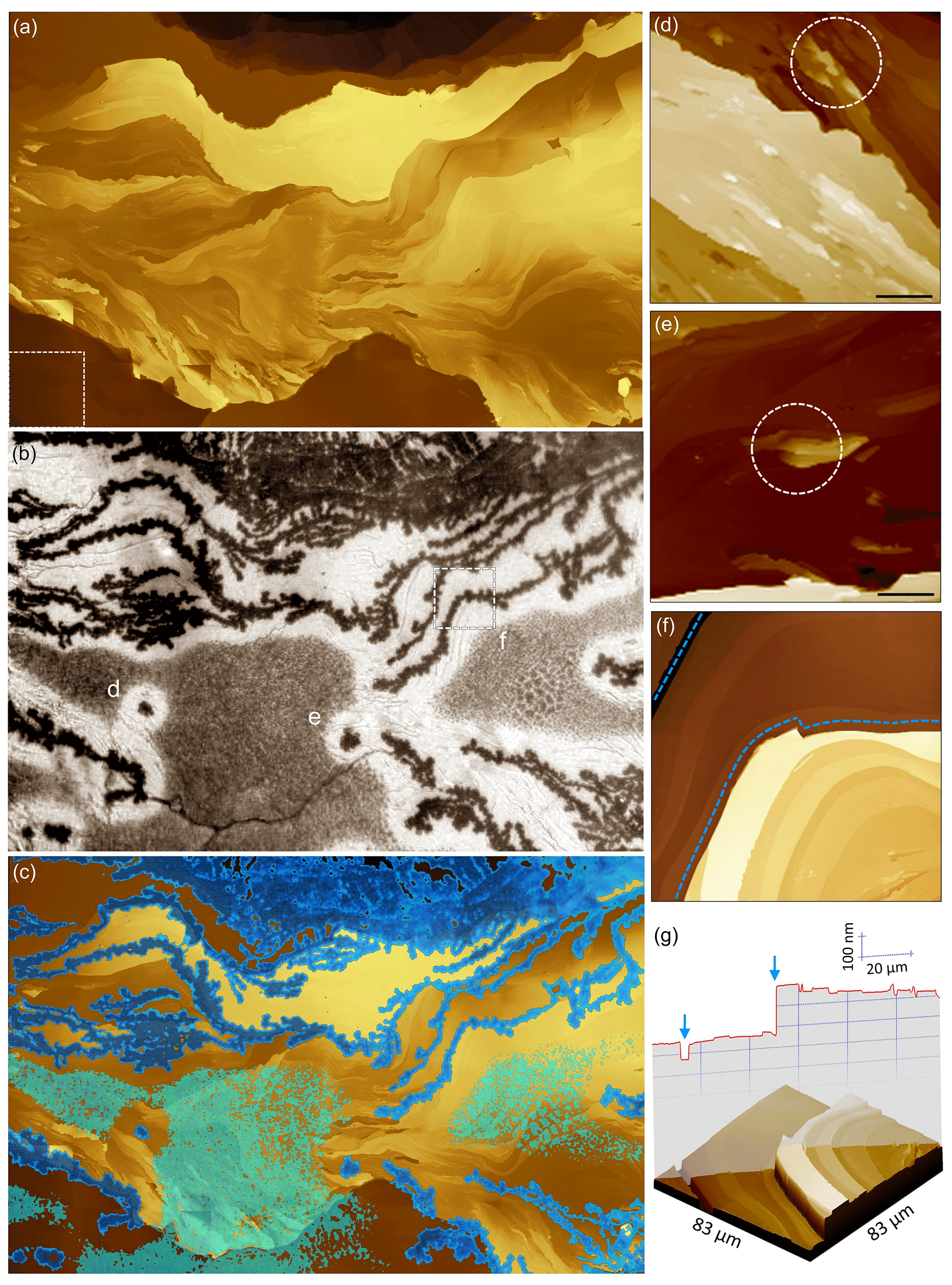
Figure 4Wide-field-of-view colocation of AFM data and optical video of ice growth at ∘C and AH g m−3. (a) A mosaic composed of 54 individual AFM images stitched together to form a topographical map spanning 750 µm × 570 µm. The box with the dashed outline on the lower left represents the 100 µm × 100 µm size of each individual AFM image. Brighter color represents higher topography. (b) An optical video frame captured over the same area as in (a) showing ice growth. Three locations of interest are marked on the optical image (d, e, f), and AFM images corresponding to their locations are shown in the panels on the right with the same labels. (c) The optical image in (b) is thresholded and false-colored and then overlaid on the AFM data shown in (a). The resulting overlay demonstrates the preference of ice formation along prominent step edges. (d, e) Two example regions where ice nucleated on the surface and grew as isolated crystals without propagating across steps. Circles with dashed outlines enclose the locations where ice nucleation occurred. Scale bars are 5 µm. (f) Planar and (g) 3D view of the region marked f in (b). Dashed lines in (f) represent the path followed by ice, and the arrows in the height profile in (g) mark locations of ice formation. Video data accompanying panel (b) can be found in Friddle and Thürmer (2019b).
4.1 Analysis of surface steps
Figure 5 illustrates the process we developed to extract step heights from the AFM data and relate those to the optically observed ice-forming locations. An AFM image (Fig. 5a) is first converted to an image of step heights (Fig. 5b), where traces outline where the step edges lie, and the value of each pixel along the trace corresponds to the step's height at that point. This step-edge image is generated by the following custom routine (Igor Pro, WaveMetrics) operating on the row and column 1D arrays of the 2D image matrix: after background subtraction, the derivative of the 1D array is taken. An edge is found when the rate of change of the differentiated array exceeds a threshold of nm mm−2, which detects step heights greater than 2 nm. Once a crossing is found, the local peak and two floor points of the derivative array are used to determine the step height from the original array. The step-edge location and height are assigned to a pixel on the new image. This process is repeated, line by line, along the rows and columns of the AFM image.
The step-edge image is interactive (Fig. 5b) to facilitate manually collecting step-height statistics over many step segments. Contiguous pixels of similar step height are grouped into clickable trace segments which change color and thickness to indicate selection (see Fig. 5d). Selection is reversible, and trace segments can be cut into smaller segments where needed to match the iced segment lengths observed optically.

Figure 5Processing video and AFM data into step-height statistics. An AFM image (a) is converted to an image of step heights (b) and compared to the corresponding optical image of ice formation (c). The step-height image in (b) is interactive in that the traces corresponding to ice-covered step segments can be selected by mouse click, shown as blue traces in (d).
4.2 Relating ice formation to step heights
Once registration between the AFM step-height image and optical image is established, the routine discussed in Sect. 4.1 is applied to collect statistics on the heights of step edges along which ice forms. As shown in Fig. 5, the selected step edges in panel d are chosen to coincide with the filaments of ice in panel c. The selected trace segments contain step-height values for each pixel along the segment. This is repeated for all the images across the desired analysis area. The selected step heights are binned into a histogram and compared against a histogram of all step heights presented in the image. Binning is counted as pixels or physical length.
Figure 6 shows an example of processed step-height data collected over 15 images, each covering 100 µm × 100 µm. Here we show histograms for ice formation on K-feldspar at four different humidities, all at a temperature of ∘C. Each histogram is derived from one video frame for each humidity which is chosen based on when ice propagation across the surface halts. Figure 6 shows the distribution of step heights for (a) all steps observed and (b) steps on which ice propagates. The ratio of these two histograms – total length of iced steps within a step-height bin over total length of all steps (within the same step-height bin) – provides the probability of finding ice on a step of a given height (Fig. 6c).
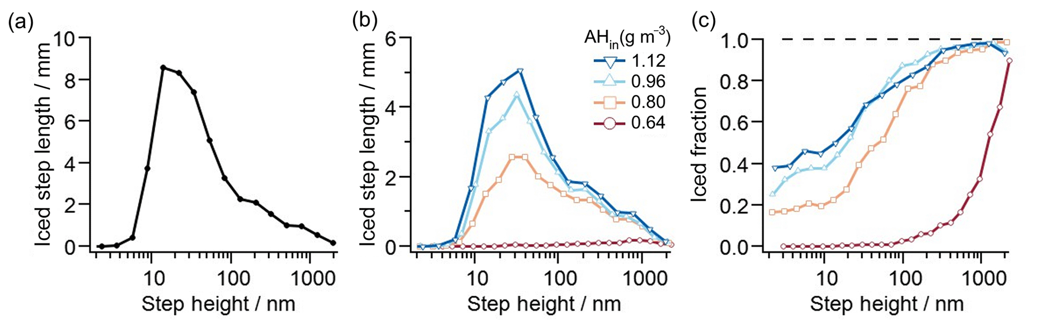
Figure 6Step-height statistics. (a) Histogram of all step heights as measured by the total length of all steps within a step-height bin. (b) Histogram of step heights as measured by the total length of iced steps within a step-height bin. The histograms evaluate 15 images, each image covering 100 µm × 100 µm. The bins are logarithmically spaced, and binning for each step height is counted up as the sum of step-edge lengths. (c) Probability of finding ice on a step of a given height, computed as the total length of iced steps within a step-height bin divided by the total length of all steps (within the same step-height bin). The data show that increasing humidity shifts the distribution to the left, thus increasing the probability of finding ice on smaller step heights. Fluctuations in the ice fraction curves, particularly at high AHin and on large steps, reflect the random dehydration of some larger step heights which are present in far fewer numbers than are smaller step heights.
The data in Fig. 6c reveal that, above saturation, ice is more likely to form along taller steps than along shorter steps. Furthermore, the sigmoidal probability distribution in Fig. 6c shifts with changing humidity: as the humidity is increased, the curve moves towards smaller step heights. As detailed in Friddle and Thürmer (2019a), the formation of ice filaments along step edges can be explained by capillary water condensation, with water filling the bottom corner where the step edge meets the underlying terrace. The orthoclase water contact angle is ∼45∘ (Karagüzel et al., 2005), and thus, at saturation, perpendicular steps of all heights will be lined with water wedges when the surface's water contact angle is ≤45∘ (Brinkmann and Blossey, 2004; Moosavi et al., 2006; Seemann et al., 2011). Therefore, steps of any height are prefilled with liquid water which can freeze in place once a nucleation event occurs anywhere along the step. This process can be viewed as an extension of the pore condensation and freezing mechanism (Christenson, 2013; David et al., 2019; Fukuta, 1966; Marcolli, 2014; Pach and Verdaguer, 2019) to higher humidity. A step-height dependence of ice growth can be attributed to two causes. First, if the probability of a given body of supercooled water to freeze at any given moment is roughly proportional to the surface area of the feldspar substrate immersed in the supercooled water, consistent with the models for immersion freezing considered in Knopf et al. (2020), then the probability of a given step-edge segment to initiate ice nucleation is roughly proportional to its height. The second cause arises from the subsequent dehydration of water wedges as denuded zones form around existing ice crystals. The taller steps contain more water and thus can retain water wedges longer than their shorter neighbors can. Hence the transformation of water wedges to ice, due to heterogeneous nucleation or contact with a nearby ice filament, has a greater window in time to occur with taller steps. This capillary-based mechanism is consistent with the ice formation shown in Fig. 4. Here, ice filaments grew when step edges maintained tall heights for extended distances, whereas isolated ice crystals were observed at step edges with short lengths, such as protrusions or depressions surrounded by flat areas.
The surface region we analyzed quantitatively is smaller than 500 µm × 300 µm; hence the temperature differences within this area are expected to be small. As can be seen directly in the images of Fig. 4, and the analysis in Fig. 6c, any possible temperature effects were not able to obscure the very strong correlation between ice-formation patterns and surface-step patterns. Hence, the rapid emergence and propagation of ice filaments is clearly not driven by temperature gradients but rather governed by the surface-step patterns. The subsequent, much slower, expansion of the clustered ice crystals decorating the steps, which was not examined quantitatively, could in principle be more affected by temperature gradients, although visual inspection of the optical images does not reveal strong evidence for this.
Typically, most aerosol particles are completely immersed in a cloud droplet even at very modest supersaturations. As discussed in detail in Friddle and Thürmer, 2019a, the step-facilitated mechanism described above is expected to be relevant when a cavity-free feldspar particle, initially devoid of ice, is suspended in air colder than −20 ∘C that becomes slowly saturated. According to Fletcher's estimate (Fletcher, 1962; Pruppacher and Klett, 1997), a humidity of RHw>130% is required for a measurable nucleation rate of water droplets with a contact angle of ≈45∘ on a planar insoluble substrate. Hence condensation of supercooled water will be confined to step edges, where the water will freeze rapidly, thus initiating ice formation.
In the discussed example of ice formation, the step-height analysis is used to corroborate the involvement of the liquid phase of water during the observed rapid formation and propagation of ice on feldspar, while the link between surface step height and the ability of an isolated aerosol particle to initiate ice nucleation is neither direct nor obvious. Nevertheless, such step-height analysis might benefit future studies in fields of material science, like corrosion and aircraft icing (Gent et al., 2000; Kreder et al., 2016), where the behavior of the examined materials is affected by the abundance of surface steps.
In the current implementation of the AFM and optical technique presented in this paper, the two microscopies are performed sequentially on the same surface area, and the data are subsequently merged for quantitative analysis of surface structure as it pertains to ice formation. Due to the limited resolution of optical microscopy, we cannot directly determine the ice nucleation site with nanometer precision. But by preparing cleavage surfaces that contain rather flat surface regions, we create configurations in which most steps are separated far enough to be optically resolved, allowing us to relate ice-propagation patterns to surface step patterns and to employ AFM to quantify the role of the steps' heights. Future experiments will explore simultaneous operation of AFM and optical microscopy, which may improve spatial localization of ice nucleation sites and resolve their morphologies. The setup described here is also applicable to studying deposition mode nucleation at below −36 ∘C and subsaturation (relevant to cirrus cloud formation) and optical observations of immersion mode nucleation on substrates. As previously demonstrated (Yang et al., 2015, 2018; Gurganus et al., 2011; Holden et al., 2019), higher frame rates than used here are imperative when the sample is immersed in water because the ice can spread to millimeter length scales on the order of milliseconds after the nucleation event. Nevertheless, higher video frame rates do not improve the resolving power of the microscope which is fundamentally restricted by the diffraction limit . In our system the small numerical aperture of our objective (NA = 0.2) follows from the large-working-distance lens required to fit within the clearance of the AFM. Dedicated microscopy systems can improve resolution by using a higher NA and by implementing blue filters to limit the wavelength λ. Ultimately, advances in high-speed AFM (HS-AFM) may be the key to direct observations of ice nucleation events. A typical commercial-AFM scan takes 10 s to 10 min depending on the flatness of the substrate, the field of view (FOV), and the desired resolution. Meanwhile at RHw≈100 % and ∘C we estimate that a new ice crystal reaches an effective diameter of 1 µm in just 6 ms.2 Progress in HS-AFM development has proven the tool to be capable of performing fast imaging of dynamic processes at nanometer resolution in various environments (Yamashita et al., 2009; Payton et al., 2016; Pyne et al., 2009; Picco et al., 2008; Kodera et al., 2010; Uchihashi et al., 2011; Casuso et al., 2010).
Lastly, the rapid propagation of ice we see on feldspar should also occur in other circumstances where extended surfaces, covered with continuous networks of steps or grooves, are exposed to a supersaturated air, providing a microscopy-based argument for avoiding surfaces with large steps or grooves in efforts to suppress aircraft icing (Gent et al., 2000; Kreder et al., 2016).
Raw AFM and optical video data supporting the findings of this study are available from Raymond W. Friddle (rwfridd@sandia.gov) or Konrad Thürmer (kthurme@sandia.gov) on request.
Videos corresponding to the optical frames presented in Figs. 2a and b, 3a, and 4b can be found online at https://doi.org/10.7910/DVN/DZUZ6P (Friddle and Thürmer, 2019a).
RWF and KT conceived of and performed the experiments, analyzed the data, and wrote the paper.
The authors declare that they have no conflict of interest.
We thank Norman C. Bartelt for insightful discussions. Sandia National Laboratories is a multimission laboratory managed and operated by National Technology and Engineering Solutions of Sandia LLC, a wholly owned subsidiary of Honeywell International Inc., for the U.S. Department of Energy's National Nuclear Security Administration under contract DE-NA0003525.
This research has been supported by the Sandia National Laboratories Directed Research and Development Program.
This paper was edited by Mingjin Tang and reviewed by Thorsten Bartels-Rausch and three anonymous referees.
Ando, T.: High-speed AFM imaging, Curr. Opin. Struc. Biol., 28, 63–68, 2014.
Brinkmann, M. and Blossey, R.: Blobs, channels and “cigars”: Morphologies of liquids at a step, Eur. Phys. J. E, 14, 79–89, 2004.
Casuso, I., Sens, P., Rico, F., and Scheuring, S.: Experimental Evidence for Membrane-Mediated Protein-Protein Interaction, Biophys. J., 99, L47–L49, 2010.
Christenson, H. K.: Two-step crystal nucleation via capillary condensation, Cryst. Eng. Comm., 15, 2030–2039, 2013.
Coluzza, I., Creamean, J., Rossi, M. J., Wex, H., Alpert, P. A., Bianco, V., Boose, Y., Dellago, C., Felgitsch, L., Frohlich-Nowoisky, J., Herrmann, H., Jungblut, S., Kanji, Z. A., Menzl, G., Moffett, B., Moritz, C., Mutzel, A., Poschl, U., Schauperl, M., Scheel, J., Stopelli, E., Stratmann, F., Grothe, H., and Schmale, D. G.: Perspectives on the Future of Ice Nucleation Research: Research Needs and Unanswered Questions Identified from Two International Workshops, Atmosphere, 8, 28, https://doi.org/10.3390/atmos8080138, 2017.
David, R. O., Marcolli, C., Fahrni, J., Qiu, Y. Q., Sirkin, Y. A. P., Molinero, V., Mahrt, F., Bruhwiler, D., Lohmann, U., and Kanji, Z. A.: Pore condensation and freezing is responsible for ice formation below water saturation for porous particles, P. Natl. Acad. Sci. USA, 116, 8184–8189, 2019.
DeMott, P. J., Prenni, A. J., Liu, X., Kreidenweis, S. M., Petters, M. D., Twohy, C. H., Richardson, M. S., Eidhammer, T., and Rogers, D. C.: Predicting global atmospheric ice nuclei distributions and their impacts on climate, P. Natl. Acad. Sci. USA, 107, 11217–11222, 2010.
DeMott, P. J., Mohler, O., Stetzer, O., Vali, G., Levin, Z., Petters, M. D., Murakami, M., Leisner, T., Bundke, U., Klein, H., Kanji, Z. A., Cotton, R., Jones, H., Benz, S., Brinkmann, M., Rzesanke, D., Saathoff, H., Nicolet, M., Saito, A., Nillius, B., Bingemer, H., Abbatt, J., Ardon, K., Ganor, E., Georgakopoulos, D. G., and Saunders, C.: Resurgence in ice nuclei measurement research, B. Am. Meteorol. Soc., 92, 1623–1635, 2011.
Fletcher, N. H.: The physics of rainclouds, Cambridge University Press, New York, 1962.
Friddle, R. and Thürmer, K.: Video microscopy of ice nucleation and growth on the (001) face of orthoclase at −30 C, Harvard Dataverse, https://doi.org/10.7910/DVN/DZUZ6P, 2019a.
Friddle, R. W. and Thürmer, K.: How nanoscale surface steps promote ice growth on feldspar: microscopy observation of morphology-enhanced condensation and freezing, Nanoscale, 11, 21147–21154, 2019b.
Fukuta, N.: Activation of atmospheric particles as ice nuclei in cold and dry air, J. Atmos. Sci., 23, 741–750, 1966.
Gent, R. W., Dart, N. P., and Cansdale, J. T.: Aircraft icing, Philos. T. Roy. Soc. Lond. Ser. A, 358, 2873–2911, 2000.
Gurganus, C., Kostinski, A. B., and Shaw, R. A.: Fast Imaging of Freezing Drops: No Preference for Nucleation at the Contact Line, J. Phys. Chem. Lett., 2, 1449–1454, 2011.
Holden, M. A., Whale, T. F., Tarn, M. D., O'Sullivan, D., Walshaw, R. D., Murray, B. J., Meldrum, F. C., and Christenson, H. K.: High-speed imaging of ice nucleation in water proves the existence of active sites, Sci. Adv., 5, eaav4316, https://doi.org/10.1126/sciadv.aav4316, 2019.
Kanji, Z. A., Ladino, L. A., Wex, H., Boose, Y., Burkert-Kohn, M., Cziczo, D. J., and Krämer, M.: Overview of Ice Nucleating Particles, Meteor. Monogr., 58, 1.1–1.33, 2017.
Karagüzel, C., Can, M. F., Sönmez, E., and Çelik, M. S.: Effect of electrolyte on surface free energy components of feldspar minerals using thin-layer wicking method, J. Colloid Interface Sci., 285, 192–200, 2005.
Kiselev, A., Bachmann, F., Pedevilla, P., Cox, S. J., Michaelides, A., Gerthsen, D., and Leisner, T.: Active sites in heterogeneous ice nucleation – the example of K-rich feldspars, Science, 355, 367–371, 2016.
Knopf, D. A., Alpert, P. A., Zipori, A., Reicher, N., and Rudich, Y.: Stochastic nucleation processes and substrate abundance explain time-dependent freezing in supercooled droplets, Npj Clim. Atmos. Sci., 3, 1–9, 2020.
Kodera, N., Yamamoto, D., Ishikawa, R., and Ando, T.: Video imaging of walking myosin V by high-speed atomic force microscopy, Nature, 468, 72–76, 2010.
Koop, T. and Mahowald, N.: Atmospheric science: The seeds of ice in clouds, Nature, 498, 302–303, 2013.
Kreder, M. J., Alvarenga, J., Kim, P., and Aizenberg, J.: Design of anti-icing surfaces: smooth, textured or slippery?, Nat. Rev. Mater., 1, 15003, https://doi.org/10.1038/natrevmats.2015.3, 2016.
Lau, K. M. and Wu, H. T.: Warm rain processes over tropical oceans and climate implications, Geophys. Res. Lett., 30, 2290, https://doi.org/10.1029/2003GL018567, 2003.
Lohmann, U. and Feichter, J.: Global indirect aerosol effects: a review, Atmos. Chem. Phys., 5, 715–737, https://doi.org/10.5194/acp-5-715-2005, 2005.
Marcolli, C.: Deposition nucleation viewed as homogeneous or immersion freezing in pores and cavities, Atmos. Chem. Phys., 14, 2071–2104, https://doi.org/10.5194/acp-14-2071-2014, 2014.
Moosavi, A., Rauscher, M., and Dietrich, S.: Motion of nanodroplets near edges and wedges, Phys. Rev. Lett., 97, 236101, https://doi.org/10.1103/PhysRevLett.97.23610, 2006.
Pach, E. and Verdaguer, A.: Pores Dominate Ice Nucleation on Feldspars, J. Phys. Chem. C, 123, 20998–21004, 2019.
Payton, O. D., Picco, L., and Scott, T. B.: High-speed atomic force microscopy for materials science, Int. Mater. Rev., 61, 473–494, 2016.
Picco, L. M., Dunton, P. G., Ulcinas, A., Engledew, D. J., Hoshi, O., Ushiki, T., and Miles, M. J.: High-speed AFM of human chromosomes in liquid, Nanotechnology, 19, 384018, https://doi.org/10.1088/0957-4484/19/38/384018, 2008.
Pruppacher, H. R. and Klett, J. D.: Microphysics of clouds and precipitation, Kluwer Academic Publishers, Dordrecht, The Netherlands, 1997.
Pyne, A., Marks, W., Picco, L. M., Dunton, P. G., Ulcinas, A., Barbour, M. E., Jones, S. B., Gimzewski, J., and Miles, M. J.: High-speed atomic force microscopy of dental enamel dissolution in citric acid, Arch. Histol. Cytol., 72, 209–215, 2009.
Rogers, R. R. and Yau, M. K.: A short course in cloud physics, Pergamon Press, Oxford, 1989.
Russell-Pavier, F. S., Picco, L., Day, J. C. C., Shatil, N. R., Yacoot, A., and Payton, O. D.: 'Hi-Fi AFM': high-speed contact mode atomic force microscopy with optical pickups, Meas. Sci. Technol., 29, 105902, https://doi.org/10.1088/1361-6501/aad771, 2018.
Rykaczewski, K., Henry, M. R., and Fedorov, A. G.: Electron beam induced deposition of residual hydrocarbons in the presence of a multiwall carbon nanotube, Appl. Phys. Lett., 95, 113112, https://doi.org/10.1063/1.3225553, 2009.
Seemann, R., Brinkmann, M., Herminghaus, S., Khare, K., Law, B. M., McBride, S., Kostourou, K., Gurevich, E., Bommer, S., Herrmann, C., and Michler, D.: Wetting morphologies and their transitions in grooved substrates, J. Phys.-Condes. Matter, 23, 184108, https://doi.org/10.1088/0953-8984/23/18/184108, 2011.
Uchihashi, T., Iino, R., Ando, T., and Noji, H.: High-Speed Atomic Force Microscopy Reveals Rotary Catalysis of Rotorless F-1-ATPase, Science, 333, 755–758, 2011.
Vali, G., DeMott, P. J., Möhler, O., and Whale, T. F.: Technical Note: A proposal for ice nucleation terminology, Atmos. Chem. Phys., 15, 10263–10270, https://doi.org/10.5194/acp-15-10263-2015, 2015.
Vergara-Temprado, J., Holden, M. A., Orton, T. R., O'Sullivan, D., Umo, N. S., Browse, J., Reddington, C., Baeza-Romero, M. T., Jones, J. M., Lea-Langton, A., Williams, A., Carslaw, K. S., and Murray, B. J.: Is Black Carbon an Unimportant Ice-Nucleating Particle in Mixed-Phase Clouds?, J. Geophys. Res.-Atmos., 123, 4273–4283, 2018.
Wang, B., Knopf, D. A., China, S., Arey, B. W., Harder, T. H., Gilles, M. K., and Laskin, A.: Direct observation of ice nucleation events on individual atmospheric particles, Phys. Chem. Chem. Phys., 18, 29721–29731, 2016.
Wang, Y., Liu, X., Hoose, C., and Wang, B.: Different contact angle distributions for heterogeneous ice nucleation in the Community Atmospheric Model version 5, Atmos. Chem. Phys., 14, 10411–10430, https://doi.org/10.5194/acp-14-10411-2014, 2014.
Welti, A., Kanji, Z. A., Luond, F., Stetzer, O., and Lohmann, U.: Exploring the Mechanisms of Ice Nucleation on Kaolinite: From Deposition Nucleation to Condensation Freezing, J. Atmos. Sci., 71, 16–36, 2014.
Yamashita, H., Voitchovsky, K., Uchihashi, T., Contera, S. A., Ryan, J. F., and Ando, T.: Dynamics of bacteriorhodopsin 2D crystal observed by high-speed atomic force microscopy, J. Struct. Biol., 167, 153–158, 2009.
Yang, F., Shaw, R. A., Gurganus, C. W., Chong, S. K., and Yap, Y. K.: Ice nucleation at the contact line triggered by transient electrowetting fields, Appl. Phys. Lett., 107, 264101, https://doi.org/10.1063/1.4938749, 2015.
Yang, F., Cruikshank, O., He, W. L., Kostinski, A., and Shaw, R. A.: Nonthermal ice nucleation observed at distorted contact lines of supercooled water drops, Phys. Rev. E, 97, 023103, https://doi.org/10.1103/PhysRevE.97.023103, 2018.
Zimmermann, F., Weinbruch, S., Schutz, L., Hofmann, H., Ebert, M., Kandler, K., and Worringen, A.: Ice nucleation properties of the most abundant mineral dust phases, J. Geophys Res.-Atmos., 113, D23204, https://doi.org/10.1029/2008JD010655, 2008.