the Creative Commons Attribution 4.0 License.
the Creative Commons Attribution 4.0 License.
 | 11 May 2020
Toward a variational assimilation of polarimetric radar observations in a convective-scale numerical weather prediction (NWP) model
Guillaume Thomas
Jean-François Mahfouf
Thibaut Montmerle
This paper presents the potential of nonlinear and linear versions of an observation operator for simulating polarimetric variables observed by weather radars. These variables, deduced from the horizontally and vertically polarized backscattered radiations, give information about the shape, the phase and the distributions of hydrometeors. Different studies in observation space are presented as a first step toward their inclusion in a variational data assimilation context, which is not treated here. Input variables are prognostic variables forecasted by the AROME-France numerical weather prediction (NWP) model at convective scale, including liquid and solid hydrometeor contents. A nonlinear observation operator, based on the T-matrix method, allows us to simulate the horizontal and the vertical reflectivities (ZHH and ZVV), the differential reflectivity ZDR, the specific differential phase KDP and the co-polar correlation coefficient ρHV. To assess the uncertainty of such simulations, perturbations have been applied to input parameters of the operator, such as dielectric constant, shape and orientation of the scatterers. Statistics of innovations, defined by the difference between simulated and observed values, are then performed. After some specific filtering procedures, shapes close to a Gaussian distribution have been found for both reflectivities and for ZDR, contrary to KDP and ρHV. A linearized version of this observation operator has been obtained by its Jacobian matrix estimated with the finite difference method. This step allows us to study the sensitivity of polarimetric variables to hydrometeor content perturbations, in the model geometry as well as in the radar one. The polarimetric variables ZHH and ZDR appear to be good candidates for hydrometeor initialization, while KDP seems to be useful only for rain contents. Due to the weak sensitivity of ρHV, its use in data assimilation is expected to be very challenging.
- Article
(9061 KB) - Full-text XML
- BibTeX
- EndNote


For a couple of decades, convective-scale numerical weather prediction (NWP) models have been developed to forecast mesoscale meteorological phenomena such as storms, wind gusts and fog, which can represent important socioeconomic threats. Nowadays, most of operational convective-scale NWP models have fine, kilometer-scale, horizontal resolutions (see review by Gustafsson et al., 2018). In the present study, the AROME-France model from Météo France (Seity et al., 2011) is used with a resolution of 1.3 km (Brousseau et al., 2016). In addition to a fully non-hydrostatic compressible set of equations, this high resolution allows an explicit representation of the deep moist convection and related dynamical parameters. As such models are run over a specific geographical region, initial conditions and lateral boundary conditions are required. Ducrocq et al. (2002) showed that accurate initial conditions can be more important than lateral boundaries to obtain skillful forecasts with such limited area models (LAMs). Several methods exist to provide initial conditions but, as explained by Gustafsson et al. (2018), better performances are obtained when a convective-scale data assimilation step is considered, compared to an initial state downscaled from a global model. In addition to observations that are representative of larger scales, observations at fine spatial resolutions and high sample frequencies are required in order to get an accurate representation of the dynamics occurring at these small scales (Benjamin et al., 2016; Brousseau et al., 2016). It is the case for data produced by weather radars: with a kilometric or finer resolution and a few minutes' temporal sampling, they are able to provide information about the intensity of precipitating systems through the horizontal reflectivity and about their dynamics from Doppler radial winds.
The dual-polarization radar technology allows us to go further in the description of precipitating systems. Seliga and Bringi (1976) were among the first to investigate the capabilities of polarimetric radars for a better understanding and representation of precipitating systems. Since then, numerous studies have shown the interest in dual-polarized (DPOL) variables to improve storm description and related processes. In a first paper, Kumjian (2013a) first describes the DPOL variables, their characteristics and ranges of values, while, in a second one (Kumjian, 2013b), he explains their usefulness for the detection of meteorological phenomena, such as hail, supercells or bright bands. DPOL variables can also be used to control the radar data quality as, for example, the determination of echo type, using a combination of several polarimetric variables. Gourley et al. (2007) use a fuzzy logic algorithm to distinguish meteorological echoes from non-meteorological ones, which is necessary for improving quantitative precipitation estimation (QPE). Detection of the major hydrometeor type in meteorological echoes can also be done with fuzzy logic algorithms, as proposed by Al-Sakka et al. (2013), for example. Another application of DPOL variables, for QPE improvements, is to use new relationships between horizontal reflectivity (ZHH), DPOL variables and rain rate, as in the Joint Polarization Experiment (Ryzhkov et al., 2005).
Nowadays, however, only the horizontal reflectivity and the Doppler wind are operationally exploited in the retrieval of initial conditions of NWP models. From a data assimilation (hereafter DA) point of view, the challenge is to extract useful information about the main control variables from ZHH, which is an indirect observation of model variables. At Météo France, a two-step method is operationally performed in the AROME-France model (Wattrelot et al., 2014). First, a radar observation operator, based on the Rayleigh's scattering theory, is used to simulate horizontal reflectivity within the model geometry. To do so, the same equation as Eq. (1) described in Sect. 2.1.2 is used. This operator accounts for scattering by rainwater, snow, primary ice and graupel (Caumont et al., 2006). Then, an interpolation of ZHH onto the radar main lobe by a Gaussian function is performed. From simulated ZHH, pseudo-profiles of relative humidity are retrieved using a 1D Bayesian inversion (as described by Caumont et al., 2010). In the second step, these pseudo-profiles are assimilated into a three-dimensional variational (3D-Var) system. In this approach, the complex linearization of the reflectivity observation operator is avoided. For any further details, please refer to Caumont et al. (2006, 2010) and Wattrelot et al. (2014). Such a procedure is also used operationally at JMA (Ikuta and Honda, 2011) and by some countries of the HIRLAM community (Ridal and Dahlbom, 2017). Other NWP models (e.g., UKV at the Met Office or HRRR at NOAA) make use of ZHH (or radar-based precipitation rate analysis in the case of the UKV) through latent heat nudging procedures (see, again, Gustafsson et al., 2018 for details). At Météo France, Doppler winds are also assimilated into the AROME-France model, but independently of horizontal reflectivities. Montmerle and Faccani (2009) show that assimilating Doppler winds clearly improves storm dynamic and precipitation forecasts, especially when low-level wind convergence is sampled. A range of studies have been also undertaken to assimilate Doppler wind and ZHH using methods based on ensemble Kalman filter (EnKF) (e.g., Tong and Xue, 2005; Dowell et al., 2011 or Bick et al., 2016), mostly for case studies. These methods avoid the linearization of observation operators and can quite straightforwardly consider hydrometeors in the control variable, but they are particularly prone to sampling noise.
In this paper, preliminary work is presented in order to prepare the assimilation of DPOL variables in a convective-scale variational DA system. Such a system is based on the minimization of a cost function, which is composed of two terms defining distances (i) between the model state and a background and (ii) between the model state in the observation space and the observations. The second term requires nonlinear (hereafter NL) observation operators in order to retrieve the model equivalent of every observation at their locations. Statistics between observed and simulated values (called innovations) are used at this stage to quantify the performance of the model in this particular space and to perform quality controls in order to produce innovation distributions that are close to a Gaussian shape, such conditions leading to optimal variational DA results. In this study, the NL observation operator described by Augros et al. (2015) is used to simulate DPOL variables from the AROME-France model. This operator is based on the T-matrix approach, which describes scattering by particles (Waterman, 1965). This approach has been used in several studies. For instance, in Bringi et al. (1986), it allows us to study the melting of the graupel by simulating the differential reflectivity ZDR. It is also used in the observation operator proposed by Jung et al. (2008), with a one-moment bulk microphysical scheme, to simulate all DPOL variables. A more complex observation operator has then been proposed by Ryzhkov et al. (2011) with a spectral microphysical scheme. Even though it leads to more physically coherent results, its computational cost is not yet compatible with operational NWP requirements.
When error Gaussianity and operator linearity are respected, the cost function of a variational DA system is close to a quadratic function for which the minimum can be easily obtained by, e.g., the method of least squares. The estimation of its gradient, which needs linearized versions of the observation operators, is then required. For operators related to precipitation, this is not straightforward as cloud microphysical processes are often highly nonlinear due to the presence of on–off switches (Sun, 2005). Furthermore, Errico et al. (2007) pointed out that these nonlinearities can severely affect the analysis. Such difficulties explain why the 1D+3D-Var approach has been initially preferred in AROME-France as discussed above. In their first attempt to assimilate ZHH in a 4D-Var, Sun and Crook (1997) did indeed find better results when simply retrieving the rain mixing ratio from an empirical relationship with ZHH instead of directly assimilating ZHH by using an NL observation operator. This approach based on empirical relationships has been more recently extended to solid precipitating species by Gao and Stensrud (2011). Other attempts of direct assimilation of ZHH with encouraging results have been made in 3D-Var (Wang et al., 2013b) and 4D-Var (Wang et al., 2013a; Sun and Wang, 2013). Nevertheless, no operational applications have been performed yet, particularly because only warm microphysical processes are considered. In this paper, before trying to linearize the highly NL DPOL observation operator, its Jacobians have been computed in order to study the sensitivity of simulated polarimetric variables to hydrometeor content perturbations.
The main goal of this paper is to study an observation operator of DPOL variables in order to determine its properties and suitability for DA, especially for hydrometeor contents initialization in the variational context of the AROME-France convective-scale NWP model. No assimilations are thus performed yet, and only results in the observation space are discussed at this point. The behavior of the operators presented in this paper in a variational DA system will be the focus of a future paper. Section 2 first describes the NL observation operator, a quantification of its errors and examples of DPOL variables simulation for different meteorological situations simulated by AROME-France. In Sect. 3, innovation statistics are discussed and used to perform quality controls on polarimetric observations. Finally, Sect. 4 focuses on the DPOL observation operator Jacobians to determine the validity of the linearity hypothesis and to quantify the sensitivity of DPOL variables to the various simulated hydrometeor contents. Conclusions and perspectives from this study are given in Sect. 5.
2.1 HDPOL description
2.1.1 Generalities
The ℋDPOL observation operator has been developed by Augros et al. (2015), and only the main characteristics are summarized here. It uses the T-Matrix method (Mishchenko and Travis, 1994) to compute the backscattering coefficients according to frequency, temperature and type of hydrometeors. The microphysical scheme used to predict hydrometeor contents is the one from the AROME model. This scheme, called ICE3, is a one-moment microphysical scheme with water vapor and five hydrometeors species: cloud droplets, rain, snow, pristine ice and graupel (Caniaux et al., 1994; Pinty and Jabouille, 1998). In the present study, only the last four have been used for the DPOL simulations, in addition to a melting species which has the characteristics of melting graupel. This melting species represents the sum of the three solid hydrometeor contents when temperature is above 0 ∘C. In this microphysical scheme, the particle size distribution (PSD) of each hydrometeor is expressed as the product between the total number concentration N0 and generalized Gamma distribution. The slope parameter used to characterize the PSD shapes depends upon the hydrometeor content M (expressed in kilograms per cubic meter), this last being the ratio between the hydrometeor content (expressed in kilograms per kilogram) and the density of an air parcel. The parameters describing the hydrometeor PSDs are given in Table 1 of Caumont et al. (2006).
Two other parameters are required for the backscattering coefficient computation: the hydrometeor shape and the dielectric constant. The latter, which describes how a material reacts to the application of electrical field, is simulated by the Debye model for raindrops (Caumont et al., 2006), and by the Maxwell–Garnett mixing formula for ice particles (Ryzhkov et al., 2011). This last formula allows us to consider solid hydrometeors as ice particles with air inclusions. For melting hydrometeor species, a dielectric constant is computed with a weighted Maxwell–Garnett mixing formula (Matrosov, 2008), which permits us to consider melting species as liquid water inclusions in ice and as ice inclusions in liquid water, depending upon liquid water and graupel fractions. For hydrometeor diameters lower than 0.5 mm, all particles are regarded as spherical (axis ratio of 1). For larger diameters, the axis ratios depend upon the hydrometeor types. Rain drops are described as spheroids, with an aspect ratio depending on diameter, in order to account for the flattening which is proportional to their size (Brandes et al., 2002). Concerning snow particles, a spheroid shape is also assumed with axis ratios linearly decreasing from 1 to 0.75 when the particle diameter increases from 0.5 to 8 mm. For higher diameters, the minimum value of 0.75 is kept. The same characteristics are used for graupel and for melting hydrometeor species, but with axis ratios linearly decreasing from 1 to 0.85. Finally, pristine ice is simulated as spherical. All these parameters have been proposed by Augros et al. (2015) as a result of sensitivity studies.
2.1.2 Simulated DPOL variables
Once the hydrometeors characteristics are defined, the T-matrix method is used to compute the backscattering coefficients for different values of particle diameters, radar elevations, temperatures and water contents (as listed in Table 1 of Augros et al., 2015). These coefficients are then integrated over diameters and stored in look-up tables to speed up computations. They are then used for the computation of the four DPOL variables of interest from the following equations:
where ZHH1 and ZVV represent, respectively, the horizontal and vertical reflectivities (in decibels relative to Z), Zhh(Zvv) the horizontal reflectivity (vertical reflectivity) expressed in radar reflectivity in linear units (mm6 m−3), λ the wavelength (in meters), the dielectric factor, function of the dielectric constant, Ni(D) the number of particles with a diameter D for the hydrometeor type i, and and the horizontal and vertical backscattering coefficients, respectively, the b exponent standing for “backward”.
with ZDR being the differential reflectivity (in decibels). This variable brings information on target aspect ratio and phase. It can be explained by its dependence upon the ratio between the horizontal and vertical reflectivity when expressed in radar reflectivity in linear units. For spherical hydrometeors (i.e., with equivalent horizontal and vertical cross sections), ZDR is equal to 0 dB. This variable will be positive (negative) when the hydrometeor horizontal dimension is larger (smaller) than the vertical one. ZDR is very sensitive to the hydrometeor dielectric factor: liquid hydrometeors will have a higher ZDR value than the solid ones with a similar shape and size distribution.
ρHV expresses the co-polar correlation coefficient:
This quantity gives information on homogeneity. When a large variety of hydrometeor sizes, shapes, phases and orientations are represented in the observed volume, ρHV values will be close to 0.
The specific differential phase KDP (in degrees per kilometer), is defined as
where expresses the difference between the real part of the forward horizontal and vertical scattering coefficients (with the f exponent meaning “forward”). This polarimetric variable expresses the phase difference between the horizontal and vertical polarized electromagnetic (EM) wave between a specific distance. In the case of spherical hydrometeors, the same amount of matter will be crossed by these two waves. Therefore, no phase difference will be observed. For nonspherical particles, the horizontally and vertically polarized EM wave will have to cross different amounts of matter, which will cause a phase difference. Because this variable only depends upon the phase difference and not upon the cross section, it is affected neither by attenuation nor by geographical masks.
2.2 Illustration of a case study
To assess qualitatively the ability of ℋDPOL to simulate DPOL variables, PPIs (plan position indicators) of the different DPOL variables are compared for one particular meteorological case. On the 10 October 2018, an important convective event strikes the South of France, mainly because of a strong southwesterly flow that took place off the coast over the Mediterranean sea. It represented an important source of humidity, and, because of low-level convergence due to orography, strong precipitation occurred over the Var, Bouches-du-Rhône and Gard departments. Such meteorological events are quite common over the Mediterranean region. For instance, Llasat et al. (2010) report that, between 1990 and 2006, 185 flash-flood events occurred around the Mediterranean basin, and about half of them happened during the autumn season. The meteorological event which took place on the 10 October 2018 produced more than 100 mm of rain in 24 h over a large area of the Var department, and locally more than 150 mm, with flash floods causing two casualties. In addition to the heavy precipitation, strong wind gusts of up to 100 km h−1 were observed. Meteorological fields from a 1 h AROME-France forecast, valid at 14:00 UTC, were used as input to ℋDPOL.

Figure 1Observed (a, c, e, g) and simulated (b, d, f, h) ZHH (a, b), ZDR (c, d), KDP (e, f) and ρHV (g, h) for the Collobrières radar the 10 October 2018 at 14:00 UTC (elevation: 2.2∘).
Figure 1 represents the observed and the simulated DPOL variables during this event, using the S-Band Collobrières radar located along the French Mediterranean coast (indicated by a dark cross), for an elevation angle of 2.2∘. The simulated hydrometeor mixing ratios from the 1h AROME-France forecast have been interpolated on the radar beam for the same elevation angle (Fig. 2). All observations have been filtered with the methodology described in Sect. 3.1. This particular radar is part of the French radar network ARAMIS (Tabary, 2007), which, in 2019, was composed of 31 weather radars, 28 having a DPOL capacity.
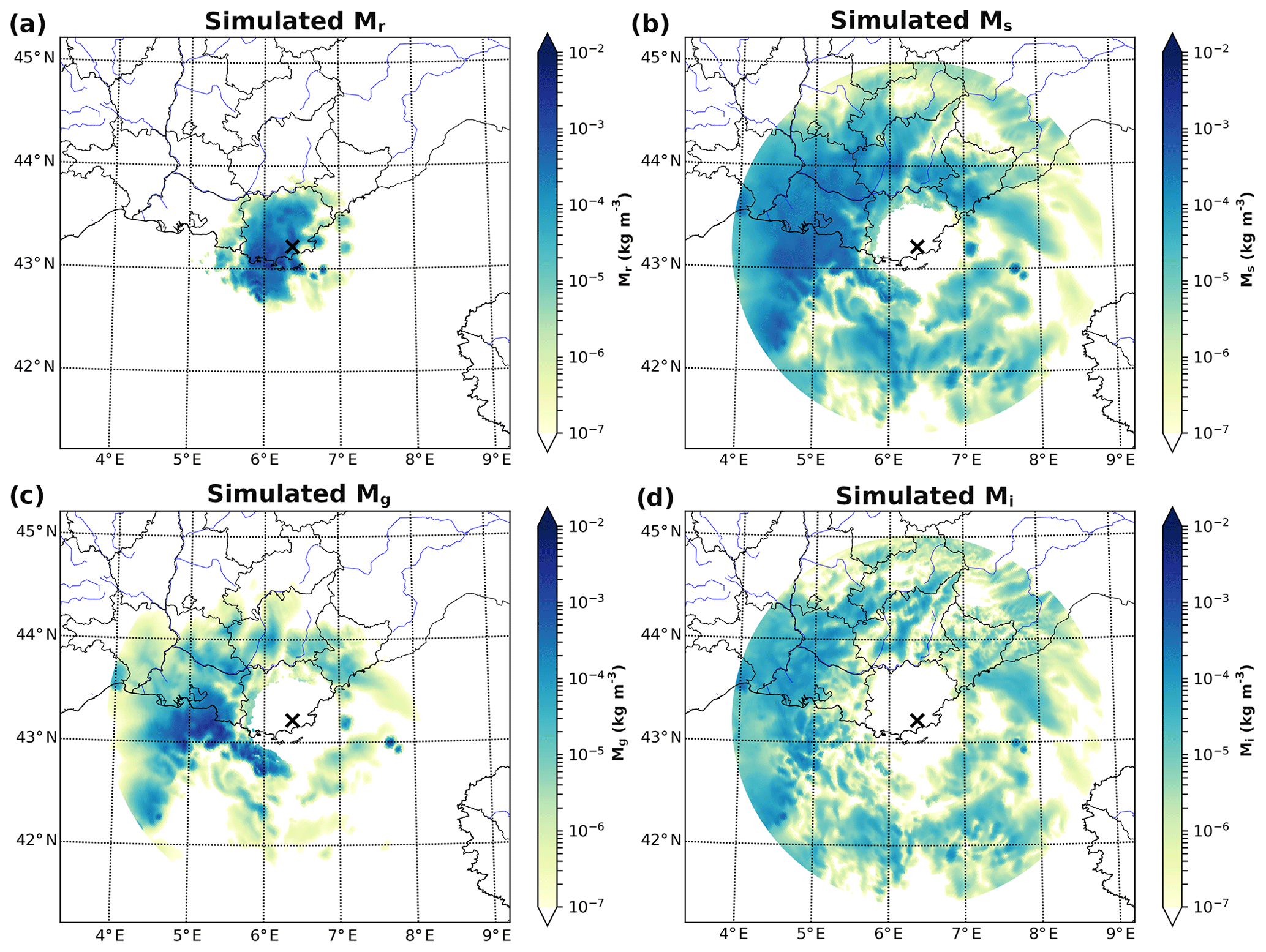
Figure 2Hydrometeor mixing ratios from a 1h AROME-France forecast valid the 10 October 2018 at 14:00 UTC for (a) rain, (b) snow, (c) graupel and (d) pristine ice.
The ZHH observations show a narrow band of very high values over the sea near the radar, locally reaching more than 50 dBZ. An area of medium to high values (20 to 40 dBZ) is located inland in the northwest quadrant, while an extended stratiform area of ZHH values above 15 dBZ is located further offshore. When examining the simulations, high values of ZHH with comparable values are also present close to the radar, however covering a wider area than in the observations. The inland area of ZHH is well represented, but with lower values than observed. Finally, for the southern part of the precipitating system far from the radar, ZHH is clearly underestimated. Since solid hydrometeors are present in this area, as displayed in Fig. 2, either AROME-France did not simulate sufficient amounts of it or such an underestimation comes from the observation operator. A combination of these two hypotheses could also explain these differences.
In agreement with areas of large ZHH values, observed ZDR can locally reach between 2.0 to 2.8 dB (Fig. 1c). Elsewhere, values are predominantly lower than 1 dB, with many small spots of higher values. Considering the simulations (Fig. 1d), the range of values are close to the observations in the area where simulated rain prevails. Nevertheless, as for simulated ZHH and contrary to what is observed, the range of values decreases with distance, which is typical of an evolution from convective liquid precipitation to more spherical solid hydrometeors. As solid hydrometeors are simulated in those areas (see, again, Fig. 2), comparison to observations clearly reflects the inability of the ICE3 microphysical parameterization to represent the observed variability of hydrometeors, particularly in the ice phase.
The observed and simulated specific differential phase KDP values are compared in Fig. 1e, f. In both cases, values up to 1.5∘ km−1 are locally displayed in the main convective area close to the radar, which is characterized by intense rainfall. As for ZDR, the area of the largest simulated ZHH values is associated with significant KDP values. Elsewhere, however, KDP values are close to zero. In general, these high amounts of zero or close to zero values for KDP or ZDR are associated with locations where the simulated ZHH is lower than 20 dBZ, corresponding to small amounts of hydrometeor contents simulated by AROME-France.
In Fig. 1g and h, only co-polar correlation coefficient values higher than 0.85 are displayed, lower ones being associated with non-meteorological echoes. Concerning the observations (Fig. 1g), the ρHV values are very close to 1 in the area of large ZHH values, mostly composed of liquid hydrometeors. Then, a ring of values between 0.9 and 0.98 is displayed, denoting the solid hydrometeors melting within the so-called bright band. Far from the radar, ρHV values increase up to 1, indicating more homogeneous solid hydrometeor distributions. In the simulation (Fig. 1h), most of the areas where ZHH is above 20 dBZ are associated with a ρHV close to 1, corresponding to very homogeneous scenes. Furthermore and contrary to what has been observed, the melting layer is not visible in the simulation. Far from the radar and in regions where the hydrometeor contents are low, the simulated ρHV decreases significantly, reaching values of less than 0.1 (not shown). It corresponds to areas where snow and ice contents are similar (see, respectively, Fig. 2b and d). Due to this specific condition, each hydrometeor type influences equally the computation of ρHV. Nevertheless, due to the large differences between the characteristics of each hydrometeor type (listed in Sect. 2.1.1), a large non-homogeneity is induced and leads to low ρHV values. Nevertheless, as such values are usually associated with non-meteorological echoes, these non-realistic simulated values are discarded. These results show the strong limitation of ℋDPOL for simulating realistic values of ρHV.
Considering all case studies (Table 1), it was generally found that realistic simulations of DPOL variables can be obtained especially in regions where liquid precipitation occur. In the presence of solid hydrometeors, the simulation of ZDR, KDP and ρHV increases in complexity and comparisons with observation show large differences. It also appears that simulated ZHH can be underestimated when only solid hydrometeors are present. The same patterns have been obtained for both S-band and C-band radar simulations, confirming the results of Augros et al. (2015). These misrepresentations are probably partly due to hypotheses done in ℋDPOL on the hydrometeor shapes and aspect ratios, on their PSDs, and on their dielectric constants. Indeed, these specified parameters might not be adequate for all meteorological situations. This is especially true for solid hydrometeors, for which the simulation of DPOL variables is particularly complex and dependent on hydrometeor characteristics simulated by the ICE3 microphysical scheme that does not describe them in enough detail.
2.3 Assessment of model errors
In order to describe the uncertainties associated with the simulation of DPOL variables, the impact of changes to three ℋDPOL main input variables has been examined. These variables are the dielectric constant, the hydrometeor aspect ratio and the hydrometeor oscillation with respect to the horizontal plane. For each type of hydrometeors, these parameters have been tested independently by applying a perturbation to the default value. For each parameter change, the look-up tables have been recomputed and a new simulation performed. Six different meteorological cases sampled by S-band radars of the French ARAMIS network (Tabary, 2007) (Table 1) have been chosen and, coupled with a set of 23 different configurations, it leads to a total of 138 different simulations. Standard deviations have been computed for each combination of input parameters listed in Table 2 and for each radar elevation. It can be noted that the oscillation parameter, for which physically realistic values described in Ryzhkov et al. (2011) have been used, has not been perturbed for primary ice which is represented by spheres in ICE3. For the dielectric constant and the hydrometeor aspect ratios, positive and negative relative perturbations have been considered.
Table 1Simulated meteorological cases used to assess simulation uncertainties. The two radars of interest operate in S-band. Times are expressed in UTC.
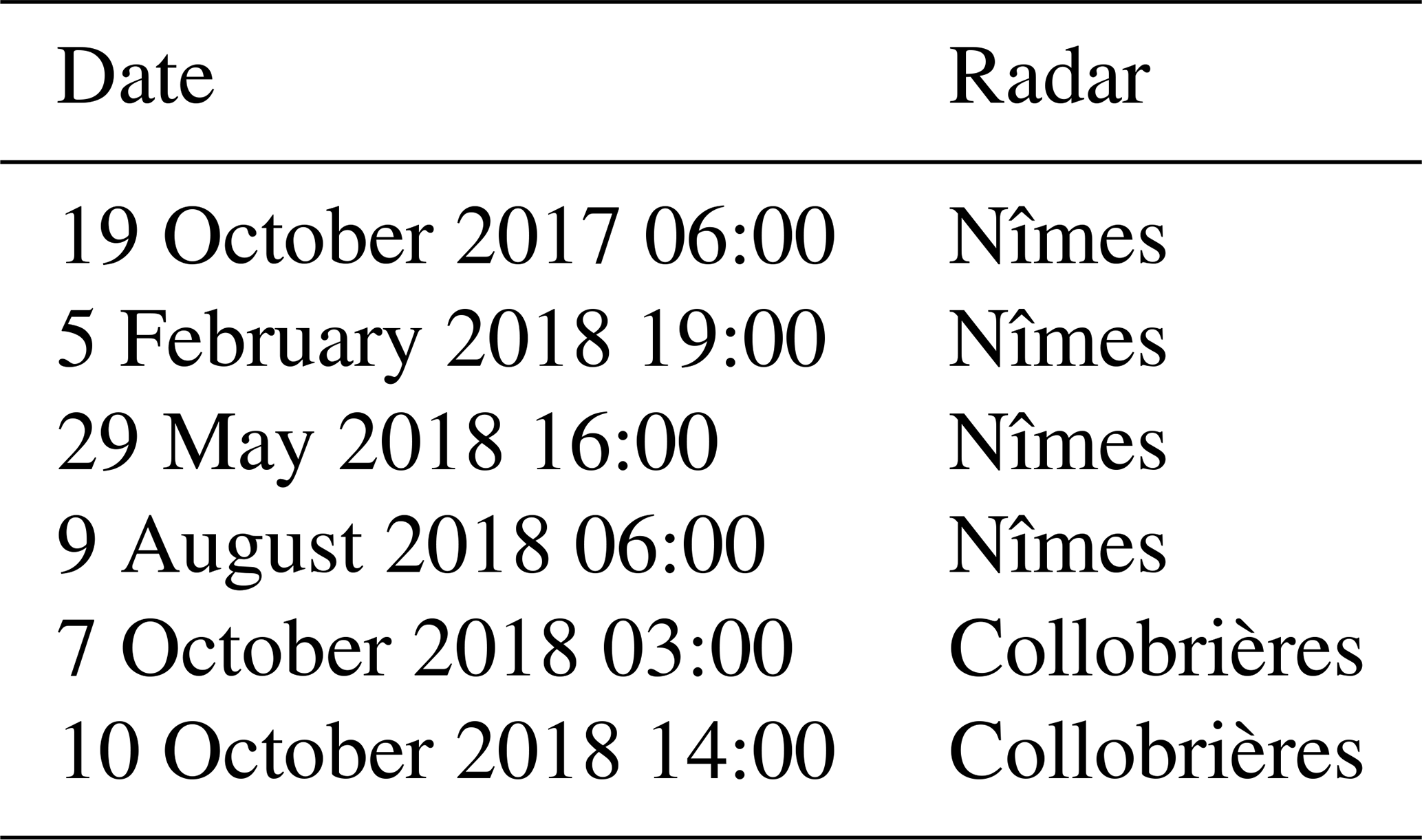
Table 2Parameters modified to study uncertainties in the ℋDPOL operator.
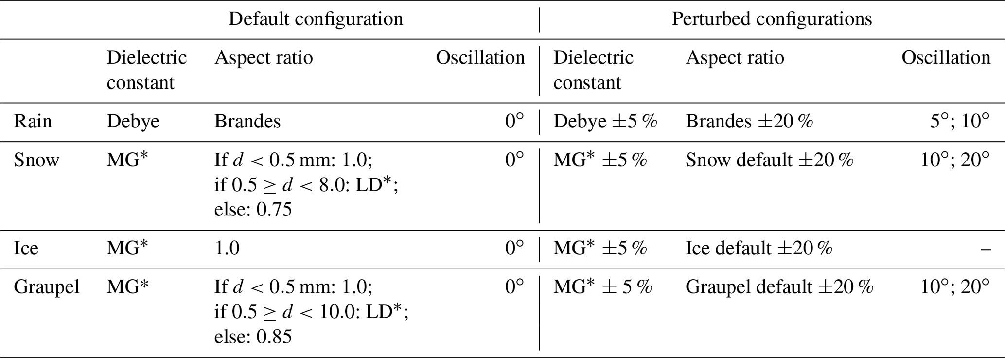
* LD stands for linear decrease and expresses the linear aspect ratio decrease with the hydrometeor diameter increase between the two threshold diameter values; MG stands for Maxwell–Garnett.
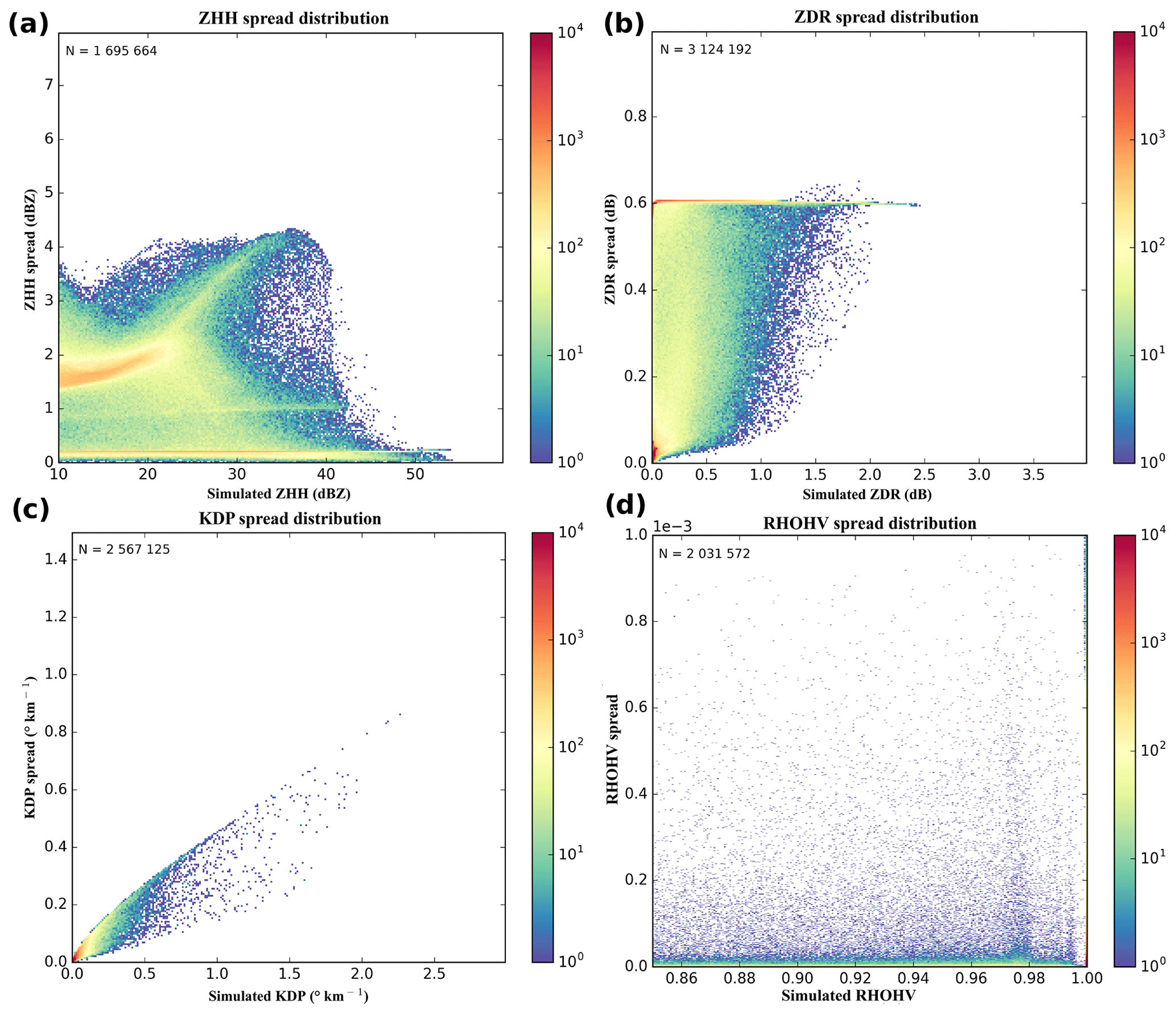
Figure 3Simulation uncertainty for (a) ZHH, (b) ZDR, (c) KDP and (d) ρHV. N represents the sample size.
The results are displayed in Fig. 3 for each DPOL variable. The first noticeable information about ZHH uncertainties is the two quasi-linear tendencies observed near 0 and 1 dBZ. The first one, around 0.1 dBZ, is induced by the perturbation of the rain aspect ratios (not shown). It was found that this behavior comes from thresholds present in the computation of the backscattering coefficients. The second quasi-linear signal, around 0.9 dBZ, appears to be mostly dependent upon the perturbation of graupel dielectric constant, without being constrained by a threshold. Overall, the uncertainty in ZHH appears to be mostly dependent upon the representation of the three types of solid hydrometeors. Indeed, each uncertainty value higher than 0.2 dBZ in Fig. 3a is associated with a perturbation of a parameter used to represent solid hydrometeors, especially the dielectric constant. For ZDR, a maximum spread around 0.6 dB is displayed. It also comes from thresholds in the backscattering coefficient computations for the rain aspect ratio. Overall, there is more variability for cases where the simulated ZDR is below 0.5 dB, which expresses a higher sensitivity of ℋDPOL to parameters describing frozen hydrometeors or small raindrops. The raindrop aspect ratio parameter explains the major part of the uncertainties appearing on ZDR simulation. Nevertheless, a small part of these uncertainties can also be explained by the dielectric constant of solid hydrometeors. Very small uncertainties have been found for ρHV simulations. Indeed, no matter the perturbed parameter, the highest uncertainty is lower than 1.10−3. Concerning KDP, a quasi-linear threshold of sensitivity is displayed. As for the spread distribution of the other DPOL variables (excepted ρHV), it comes from the rain aspect ratio. This parameter also explains the major part of the variability of KDP uncertainties.
The results of these sensitivity tests show that ZHH is sensitive to assumptions made on the simulation of the backscattering coefficients for the different hydrometeor types, especially for the solid ones. Indeed, it appears that ZHH uncertainties are, for their major part, explained by the hypotheses regarding the dielectric constant of solid hydrometeors. Then, this could explain the underestimates found for simulated ZHH in the presence of solid hydrometeors (Fig. 1). By contrast, the other DPOL variables appear to be less sensitive to choices made for solid hydrometeors than for liquid ones. Even if DPOL variables are highly influenced by hydrometeor dielectric constants, they are also known to be dependent upon hydrometeor shapes. For ZDR and KDP, uncertainties have been found in the simulations for raindrop aspect ratio perturbations, while, for solid hydrometeors, no uncertainties or very small ones have been found by perturbing their aspect ratios. These results can be explained by the one-moment microphysical scheme ICE3 that characterizes hydrometeors and related processes. Indeed, the PSDs are deduced from the hydrometeor contents and from constant parameters in order to characterize the generalized Gamma distributions (see, again, Table 1 in Caumont et al., 2006). Concerning the hydrometeor shapes, oblate spheroids appear to be a good approximation of raindrop shapes, while it might be very limiting for solid hydrometeors that exhibit a large diversity of shapes. For example, Liu (2008) proposed the use of 11 solid particle shapes along with the discrete dipole approximation (DDA) method in order to compute more realistic scattering. Clearly, the T-matrix method is comparatively limited, as it is only applicable to spheres and rotationally symmetrical particles.
A similar study to the one presented here with S-band radars has been conducted with 11 different meteorological cases, but with C-band radars (not shown). Comparable results have been obtained, the spread being nevertheless slightly larger for ZHH values higher than 30 dBZ, for ZDR values higher than 1 dB and for the total range of KDP values. These results highlight the dependence of simulated DPOL variables upon the wavelength. As suggested by the range of values affected by a larger spread, Mie diffusion occurs for large hydrometeors with C-band radars.
Nevertheless, despite choices made in ℋDPOL and, as discussed in Sect. 2.2, the polarimetric observation operator is able to simulate DPOL variables in the presence of liquid and solid hydrometeors, as shown for instance in Fig. 1d for ZDR. As discussed at the end of the next section, model errors that have been quantified in this sensitivity study will be considered for specifying a proxy of the observation error standard deviations, in addition to measurement and representativeness errors. Such values could then be used as diagonal elements of an observation error covariance matrix R necessary for variational DA studies.
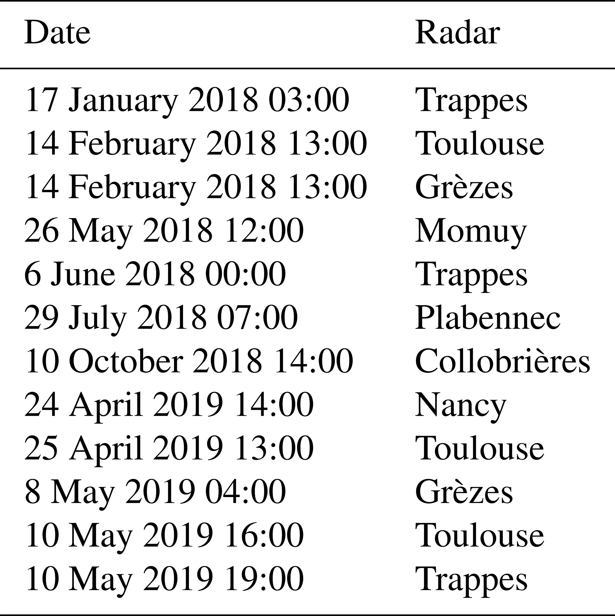
As explained previously, the optimality of variational DA requires Gaussianity of errors. For that purpose, innovation statistics (differences between observation and model counterparts) are examined. An ad hoc quality control could then be defined in order to improve Gaussianity. In this study, such statistics have been computed for 12 contrasted meteorological cases, encompassing convective and stratiform precipitation. Among those cases, only the Collobrières case has been observed by an S-band radar, while the others have been sampled by C-band radars (see Table 3). The geographical radar location is given in Fig. 1 from Tabary (2007).
Table 3Meteorological cases selected to study the innovation statistics of DPOL variables. Times are expressed in UTC.
3.1 Data preprocessing
Several filters are applied to the observations, principally to remove non-meteorological echoes and regions of too low a signal-to-noise ratio (SNR). Non-meteorological echoes are filtered using an echo type determination algorithm developed by Gourley et al. (2007). A second filter removes possible remaining ones by excluding pixels for which ρHV values are lower than 0.85. The third filter uses a threshold on SNR values. Tabary et al. (2013) explain that polarimetric variables are very sensitive to noise and, for safety reasons, all pixels with an SNR value lower than 15 dB are discarded. Finally, a median filter is applied to remove all residual isolated noisy data.
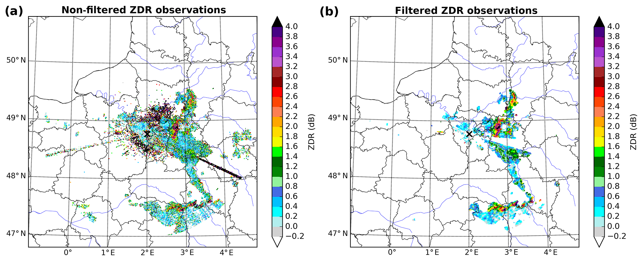
Figure 4Filtering effects on ZDR observed by the Trappes radar during a convective event on June 2018 06:00 UTC, for an elevation of 0.4∘.
Figure 4 shows the effects of these filters on ZDR values observed during a convective event that occurred in the Paris area. In Fig. 4a, ground clutters, characterized by high ZDR values, are present close to the radar. Medium to very strong values can also be observed along two different azimuths. These patterns are often due to WLAN (wireless local area network) interferences. In Fig. 4b, those patterns are not present anymore, thanks to the application of the various filters. One can note that other features, located far from the radar, have also been removed. They correspond to data with SNR values lower than 15 dB.
3.2 Results
In order to quantify the effect of the filters, innovations have been computed on non-filtered and filtered observations. Figure 5a shows that filtering the ZHH observations leads to a small decrease in the bias and standard deviation values: from 3.22 to 3.18 dBZ and from 11.44 to 11.15 dBZ, respectively. Concerning ZDR (Fig. 5b), the filtering leads to strong changes in the innovation statistics. Indeed, the bias decreases from 0.37 to 0.33 dB, while the standard deviation drops from 1.26 to 0.55 dB. For KDP (Fig. 5c), filters do not influence innovation statistics. The use of filters mostly affects the negative part of ρHV innovations (Fig. 5d), by removing simulated values close to 1. Overall, these results show small modifications of innovations statistics, except for ZDR. For the latter, quality controls appear to be critical and allow us to discard about 43 % of spurious ZDR observations. The innovation distributions appear to have a Gaussian shape for ZHH and ZDR, while it is not the case for KDP and ρHV.
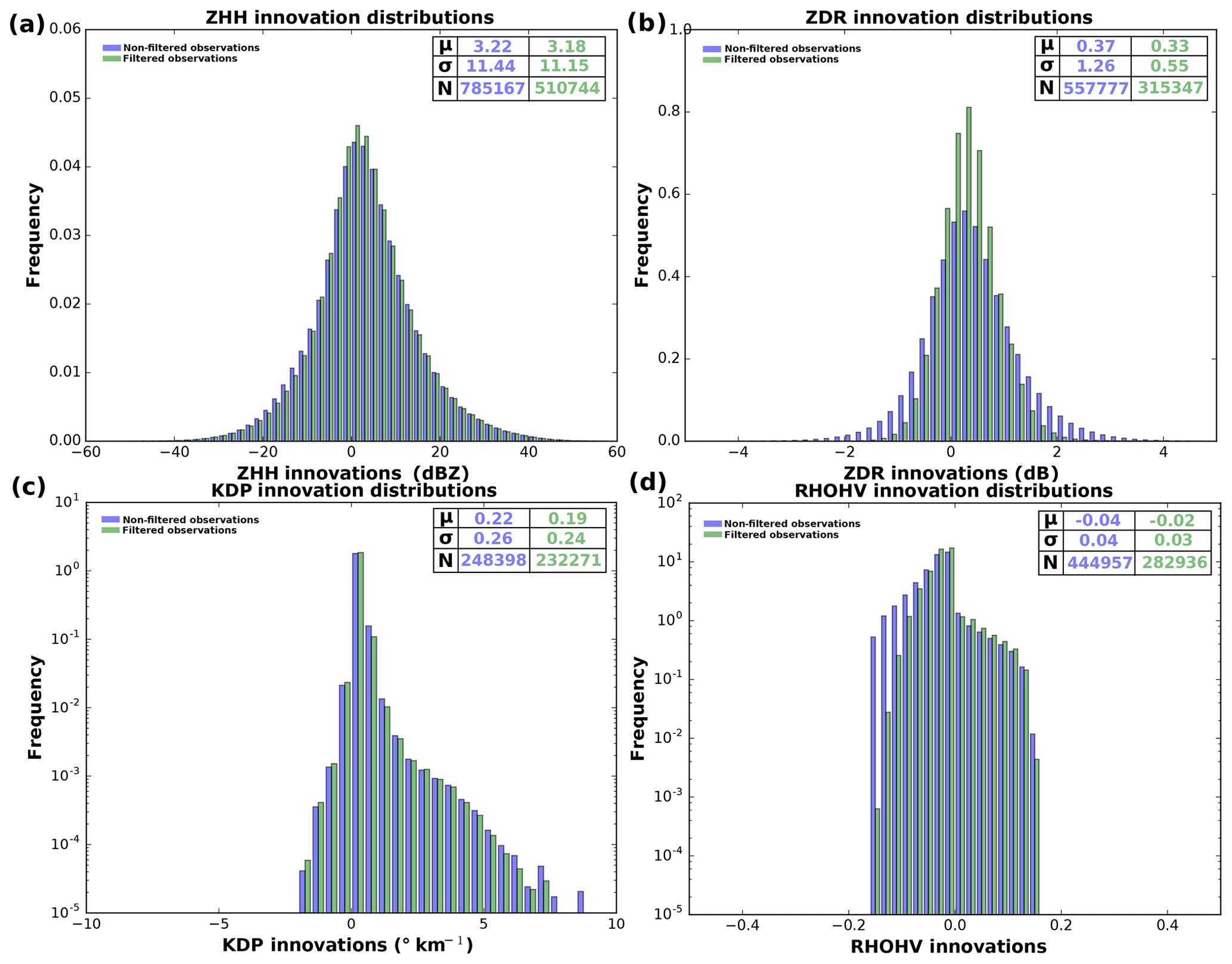
Figure 5Innovations without (blue histograms) and with (green histograms) filters on observations for (a) ZHH, (b) ZDR, (c) KDP and (d) ρHV. μ represents the innovation bias, σ the innovation standard deviation and N the sample size.
In order to study if these conclusions depend on the hydrometeor phase, innovation statistics have been computed for different vertical levels. Figure 6 represents such distributions over altitude for the studied DPOL variables, when filters are applied. The ZHH innovation distribution (Fig. 6a) exhibits a positive bias which tends to slightly increase with altitude. It expresses underestimations done in the presence of solid-phase hydrometeors that have been already noted, especially for pristine ice which is present at high altitudes. One can note a small asymmetry present in the innovation distribution below 4 km. Indeed, in this part of the atmosphere, a larger number of innovation values are represented in the distribution between 40 to 60 dBZ than in the symmetrical negative part. Depending upon the meteorological situation, this range of altitudes correspond to the melting layer. Large positive innovations in this particular area can highlight melting layer misrepresentations in ℋDPOL which lead to ZHH underestimations. Same phenomenon is present for other DPOL variables for this range of altitudes, especially for the differential reflectivity. About ZDR (Fig. 6b), a positive bias indicates an underestimation in the simulations. Nevertheless, for altitudes higher than 10 km, the bias drops to nearly 0 dBZ values. Concerning KDP (Fig. 6c), innovations show a small bias which slightly increases with altitude. Below 7 km, the innovation spread shows underestimations and overestimations done in simulations, while above 7 km, innovations are always positive, indicating systematic KDP underestimations with ℋDPOL at those levels, in the presence of solid hydrometeors. By contrast, ρHV innovation distributions (Fig. 6d) show a negative bias, indicating overestimations in the simulations.
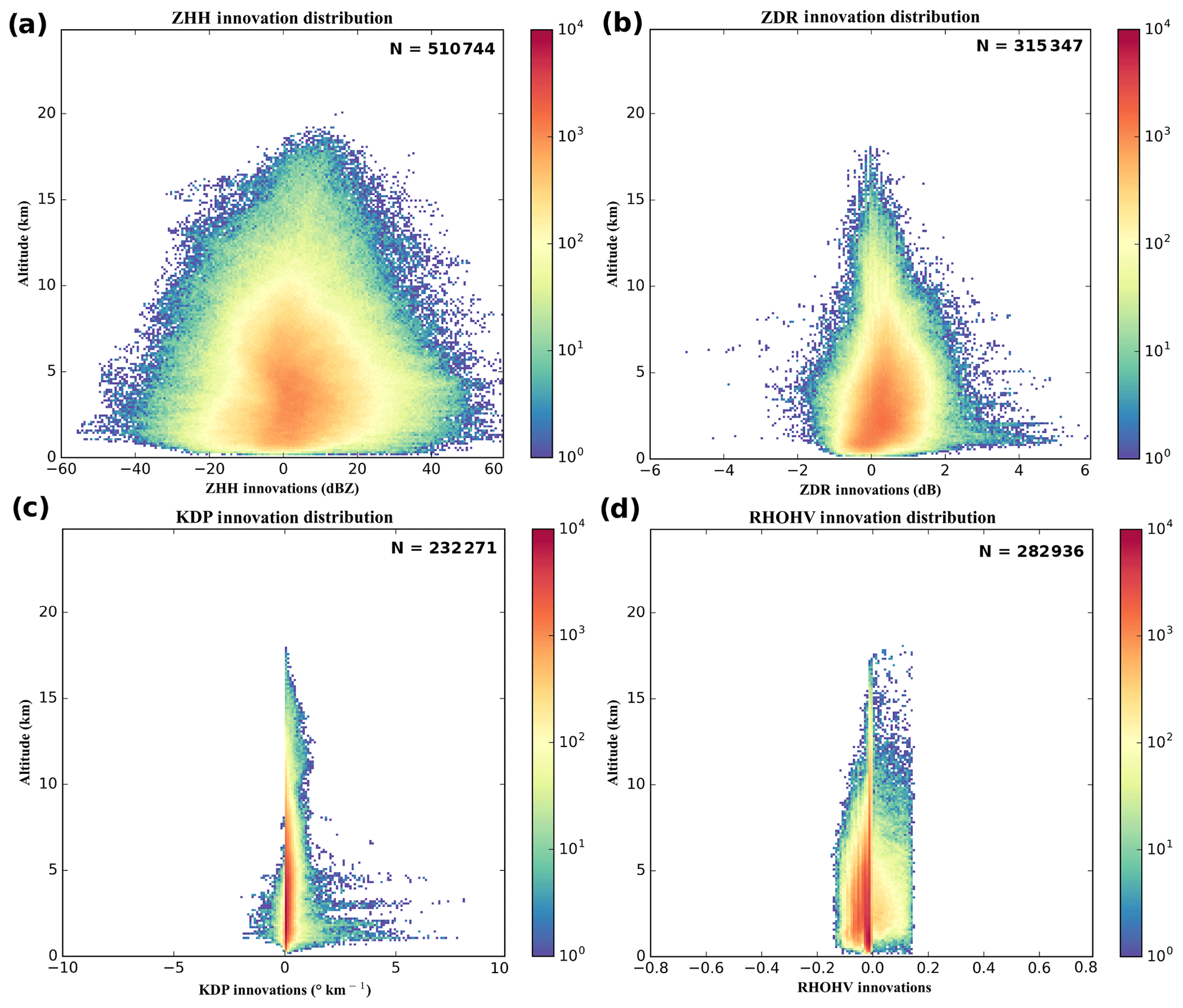
Figure 6Innovation distributions over altitude for (a) horizontal reflectivity (ZHH), (b) differential reflectivity (ZDR), (c) specific differential phase (KDP) and (d) co-polar coefficient (ρHV). N indicates the sample size for each DPOL variables.

Figure 7First-guess (a, c) and observation distributions (b, d) for ZHH (a, b) and ZDR (c, d).
To better understand the behavior of innovations, separated distributions of simulated and observed values are examined. Figure 7 represents the distributions of first-guess and observation distributions for ZHH and ZDR. Concerning ZHH, first-guess and observation distributions (Fig. 7a and b, respectively) look very similar for values above 20 dBZ, which shows the ℋDPOL capacity to simulate such variables in the presence of medium to heavy precipitation. Between 10 and 20 dBZ, the number of observations is larger than the simulated ones, which reflects the ℋDPOL underestimation of ZHH in the solid phase already pointed out. Between 0 and −10 dBZ, the number of simulated values is higher than the observed ones, denoting ℋDPOL capacity to simulate small values in the presence of very low hydrometeor contents. Simulated values below −10 dBZ, which are generally close to the radar SNR, cannot be considered for the assimilation and thus have been discarded.
Concerning ZDR, first-guess and observation distributions (Fig. 7c and d, respectively) appear to be quite different. For positive ZDR values, both distributions are similar, especially for small values. Indeed, the higher the ZDR value is, the larger is the difference between first-guess and observation distributions. It comes from the complexity of ZDR simulations, especially in the presence of solid hydrometeors, where large underestimations occur. In addition, a large fraction near 0 dB in the simulations is not represented in the observations. Finally, the negative ZDR values in the observations have not been simulated by ℋDPOL. They correspond to hydrometeors with larger vertical axes than horizontal ones. As such a hydrometeor shape is not represented in ℋDPOL, simulated ZDR cannot reach negative values. Physically, such values are usually associated with particular situations in convective events which can cause preferential vertical orientation of solid hydrometeors, as electrification processes (Kumjian, 2013a).
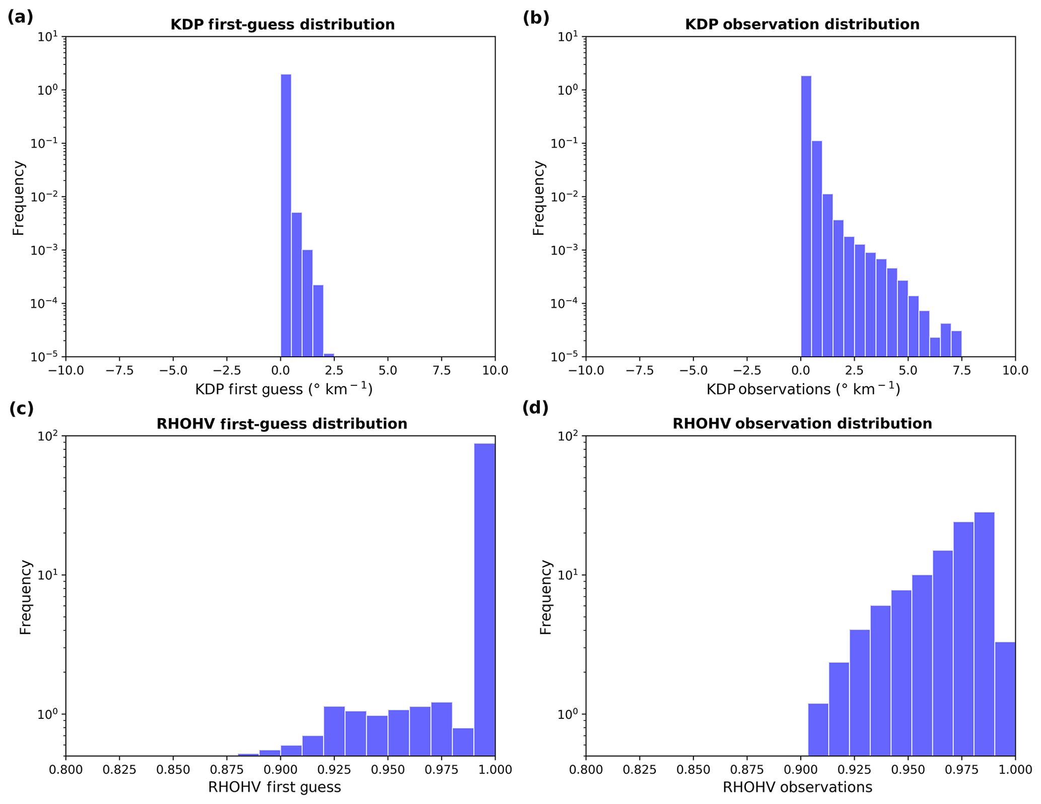
Figure 8 is similar to Fig. 7, but for KDP and ρHV and only in the presence of liquid hydrometeors. The KDP first-guess distribution (Fig. 8a), in comparison to the observations distribution (Fig. 8b), emphasizes the large underestimations of the simulations. Indeed, the largest simulated KDP values are about 2.0∘ km−1, while the maximal observed one reaches 7.5∘ km−1. This leads to an innovation distribution which is far from Gaussian, with a strong positive bias (see Fig. 5c). To be able to assimilate this variable, a strict data selection should be done. Regarding ρHV, most of simulated values are very close to 1.0 (Fig. 8d), while the observed values range between 0.90 and 1.0. These results reinforce the lack of variability of simulated ρHV values found in Sect. 2 and lead to an innovation distribution which is far from Gaussian (see Fig. 5d).
These innovation statistics can also be used to define an approximation of observation standard deviations. Indeed, Errico et al. (2000) explain that, if innovation PDFs are normally distributed,
with being the variance of the innovation PDFs and and being, respectively, the observation and the background error variances. In order to obtain a very first approximation of the observation standard deviation σo, it can be assumed that σo and σb are equivalent. In such conditions,
Values of σo(ZHH)=7.88 dBZ, σo(ZDR)=0.39 dB, km−1 and σo(ρHV)=0.02 have been found. Nevertheless, such values must be refined, especially for KDP and ρHV, for which Gaussianity has not been found in the innovation PDFs.
4.1 Perturbation size determination
As explained in the introduction, the adjoint of the linearized observation operator is required in the formulation of the gradient of the cost function. ℋDPOL being an observation operator which deals with cloud microphysical processes, numerous highly nonlinear processes are present. In this study, the linearized version of ℋDPOL, denoted H, has been estimated by its Jacobians, computed through the use of the finite difference method:
with ℋ representing the nonlinear version of ℋDPOL and δM a perturbation of the hydrometeor content M.
Then, the Jacobian matrix can be estimated as follows:
with k representing the model level number and l the radar elevation and Mi,k being the hydrometeor content (in kilograms per cubic meter) associated with type i.
First of all, it is important to evaluate the validity of the linear regime, according to the size of the perturbation δM. Duerinckx et al. (2015) proposed a method for examining the absolute value of the difference of computations between equivalent positive and negative perturbations. They explain that, as long the problem stays in a linear regime, this difference should remain close to zero. In this study, hydrometeor contents can span a wide range of values (several orders of magnitude). As a consequence, the perturbations are chosen as a fraction of the hydrometeor content (instead of a fixed value). The optimal value of perturbation for the Jacobians has been estimated in the model space. As ℋDPOL computes the DPOL variables independently for each pixel of the domain before being interpolated on the radar beam, only the diagonal elements of the Jacobian matrix are examined, since pixels, in model space, are uncorrelated both horizontally and vertically. These computations have been done for several profiles but, for illustration, only a single profile associated with convective precipitation is presented. Figure 9 shows how the optimal rain content fraction δMr has been chosen to compute the Jacobians δZHH∕δMr. One can note that the optimal rain content fraction lies between 10−2 and 10−6 g m−3.
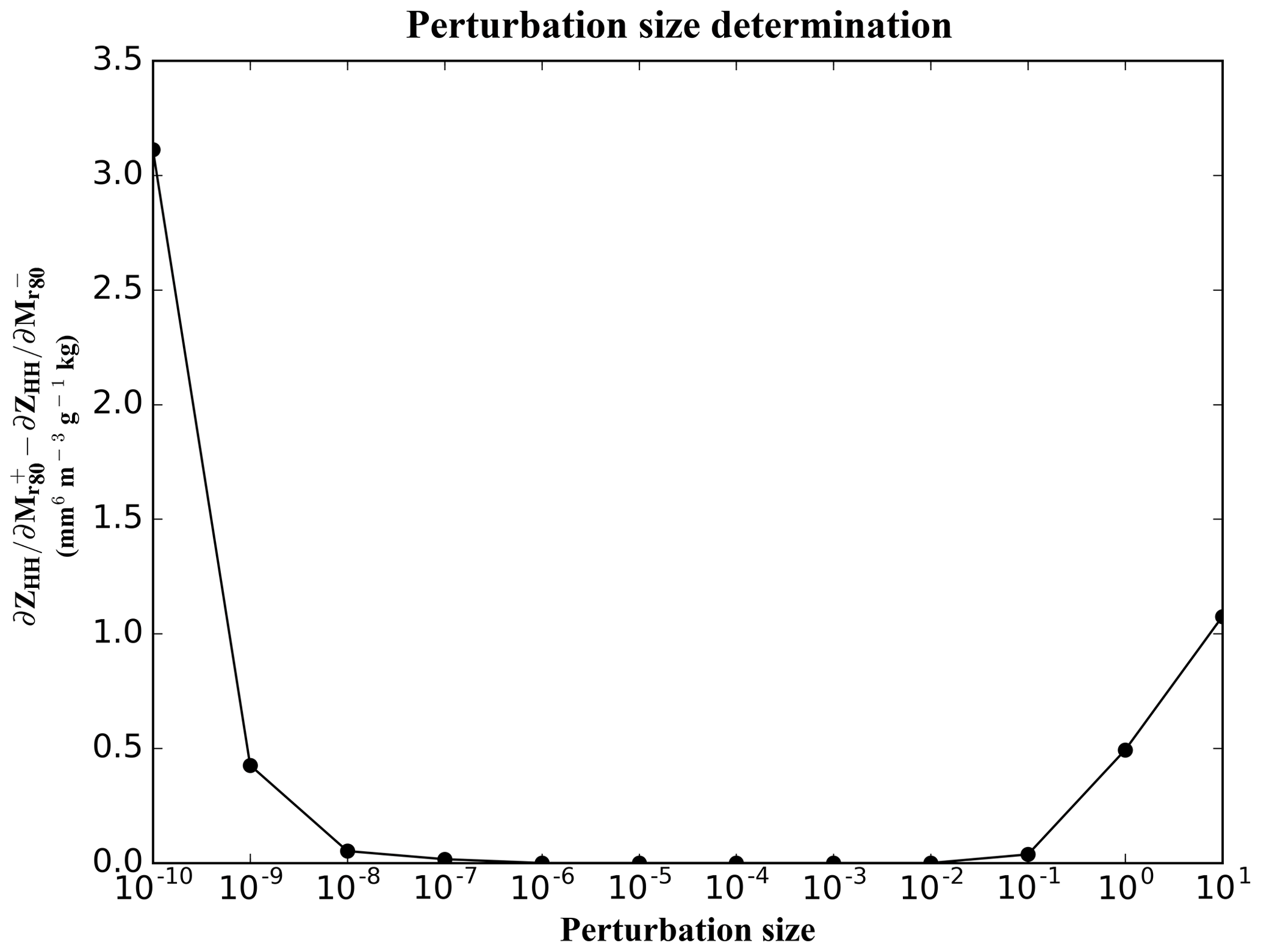
Figure 9Difference between at model level 80 (about 1 km of altitude), estimated with positive and negative perturbations as a function of the perturbation size δMr.
For each hydrometeor type, a single fraction of hydrometeor content has been determined for all DPOL variables, by selecting the highest optimal fraction size in common between the four DPOL variables. It was found that the optimal fraction size is 10−5 g m−3 for rain and primary ice contents, while 10−4 g m−3 is more suitable for snow and graupel contents.
4.2 Jacobian profiles in the model space
The information provided by the DPOL variables depends upon the interaction of the different hydrometeors scanned by the radar beam. A primary step towards understanding DPOL variable Jacobians is to exclude the radar beam effect. In that case, it is proposed to first consider the diagonal elements of the Jacobian matrix computed in model space. The perturbation used at each level in the Jacobian computation is applied as follows:
with representing the perturbed hydrometeor content at level k, Mk the hydrometeor contents at level k and δM the optimal fraction of hydrometeor contents previously chosen. The product MkδM represents the perturbation applied at level k. Once the Jacobians are computed, a normalization by 10 % of the hydrometeor profile is applied. This procedure allows a comparison between Jacobians of a given DPOL variable for different hydrometeor types.
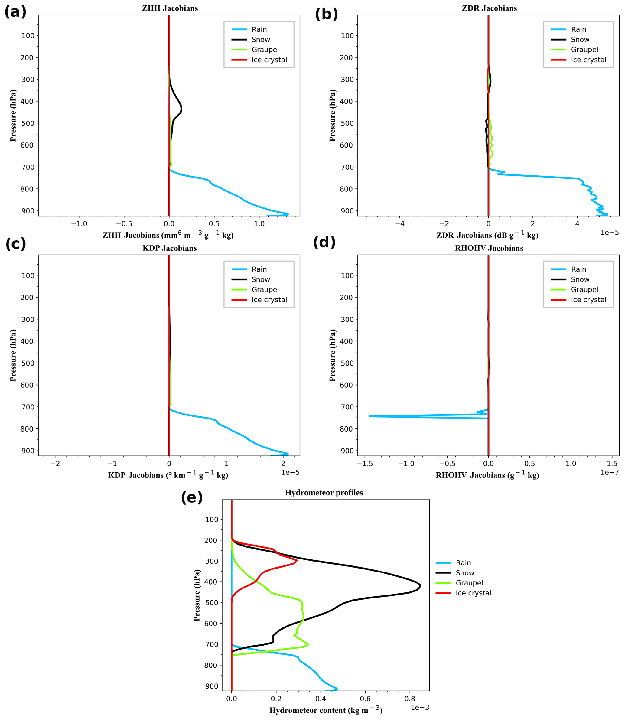
Figure 10(a) ZHH Jacobians, (b) ZDR Jacobians, (c) KDP Jacobians and (d) ρHV Jacobians; (e) represents hydrometeor content profiles, associated with a convective event which struck the Hérault and Gard departments on the 19 October 2017 06:00 TU. The Jacobians presented here are normalized by 10 % of the hydrometeor contents. .
Figure 10 presents the DPOL variables Jacobians computed from a particular profile extracted within a convective cell forecasted by AROME-France (Fig. 10e). It shows that an increase in hydrometeor content leads to higher ZHH Jacobian values (Fig. 10a).2 It is explained by the fact that reflectivity is proportional to the total hydrometeor cross section (see Eq. 1). Nevertheless, due to different dielectric constants, Jacobian values are different according to the hydrometeor type. Indeed, ZHH appears to be more sensitive to rain content perturbations, while its sensitivity to snow content perturbations is about 1 order of magnitude lower. ZHH sensitivities to graupel and pristine ice perturbation are even lower.
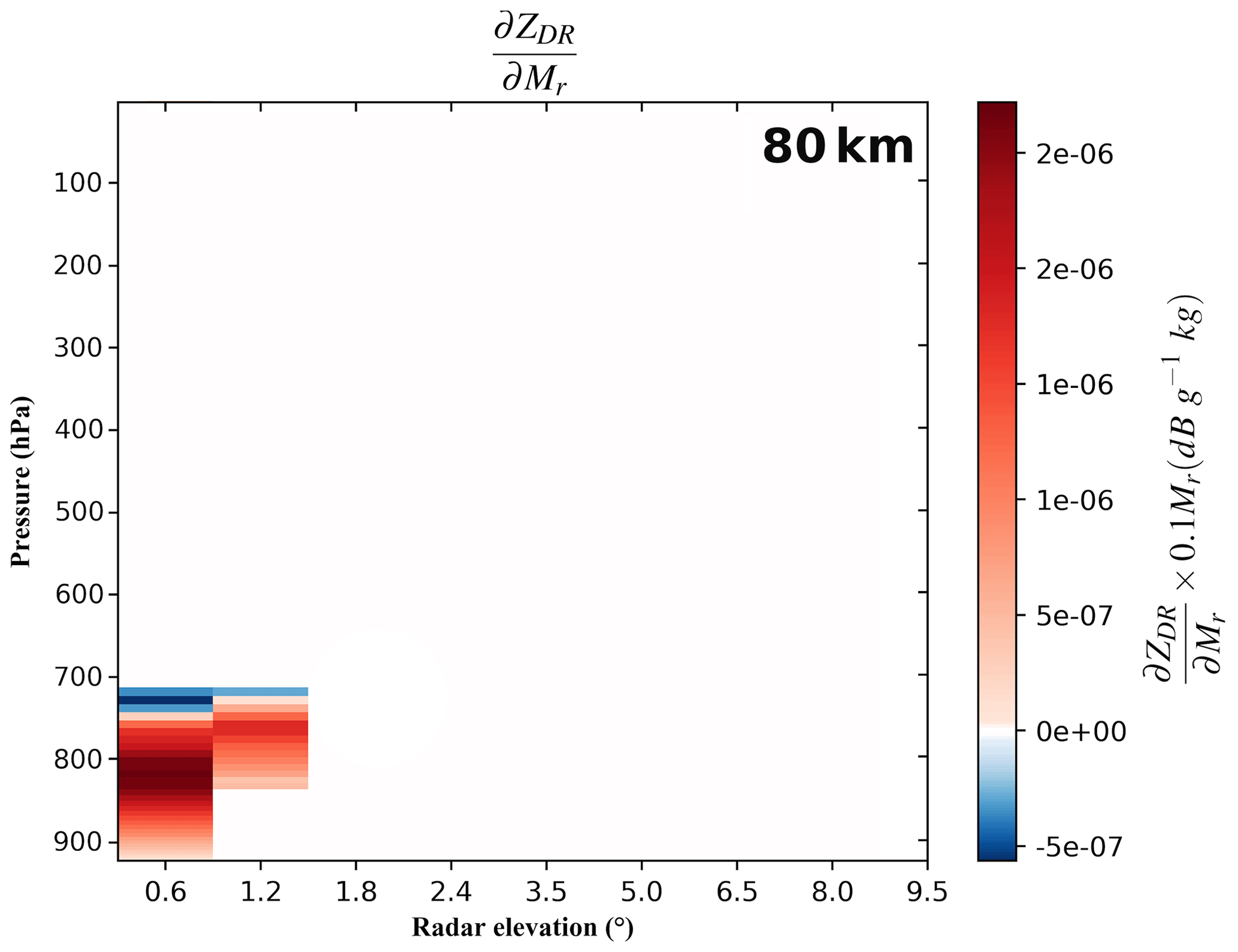
Figure 11ZDR Jacobian for a rain content perturbation associated with the AROME hydrometeor profile shown in Fig. 10 located at 80 km from the radar. The Jacobians are normalized by 10 % of the hydrometeor content.
Contrary to ZHH, which mostly depends on the total cross section and the dielectric factor, other DPOL variables are also strongly dependent upon hydrometeor characteristics, such as their shape or their orientation. ZDR, for instance, as previously explained, depends upon hydrometeor dielectric constant and shape as well as the proportion of each type of hydrometeors with respect to the total hydrometeor content. Figure 10b shows ZDR Jacobians for different hydrometeor content perturbations. Raindrops being simulated as oblate spheroids, their larger horizontal cross section compared to the vertical one leads to positive ZDR Jacobians for a rain content perturbation (Fig. 10b). For other hydrometeor content perturbations, Jacobian values can be negative. Such values can be observed for ice content perturbation around 300 hPa and for snow content perturbation between 400 and 700 hPa. For pristine ice, the negative Jacobian values are due to the increase in spherical particles in the presence of snow (see Fig. 10e). It causes a small decrease in the proportion of nonspherical particles in the total hydrometeor content and then a decrease in ZDR. By contrast, an increase in snow content in the same part of the atmosphere causes positive Jacobian values due to the increase in nonspherical particles in the total hydrometeor content. From 300 to approximately 600 hPa, the graupel content is increasing, while snow amounts are increasing between 300 and 400 hPa and then decreasing (Fig. 10e). Between these pressure levels, the ZDR Jacobian associated with a snow content perturbation is decreasing and reaches negative values. As the graupel dielectric constant is higher than for snow, it becomes predominant in the Jacobian values. So, even if there is an increase in snow content, which is characterized by flatter particles than graupel, their presence leads to a reduction in ZDR when it is not the prevailing hydrometeor type. One can note that the negative values of between 300 and 600 hPa show vertical oscillations which are likely due to changes in proportions of the different hydrometeor types. Below 600 hPa, the snow content becomes lower than the graupel one. Since an increase in snow adds flatter particles, it also leads to an increase in ZDR Jacobian values in this part of the atmosphere. Approximatively below 700 hPa, rain content is increasing and, because of the large predominance of the liquid water dielectric constant over the one from other hydrometeor types, the values drop to zero, even though snow is still present near the melting layer. Overall, as for ZHH, the highest Jacobian values are obtained for rain content perturbations, due to the large difference in the dielectric constant between liquid water and solid hydrometeors.
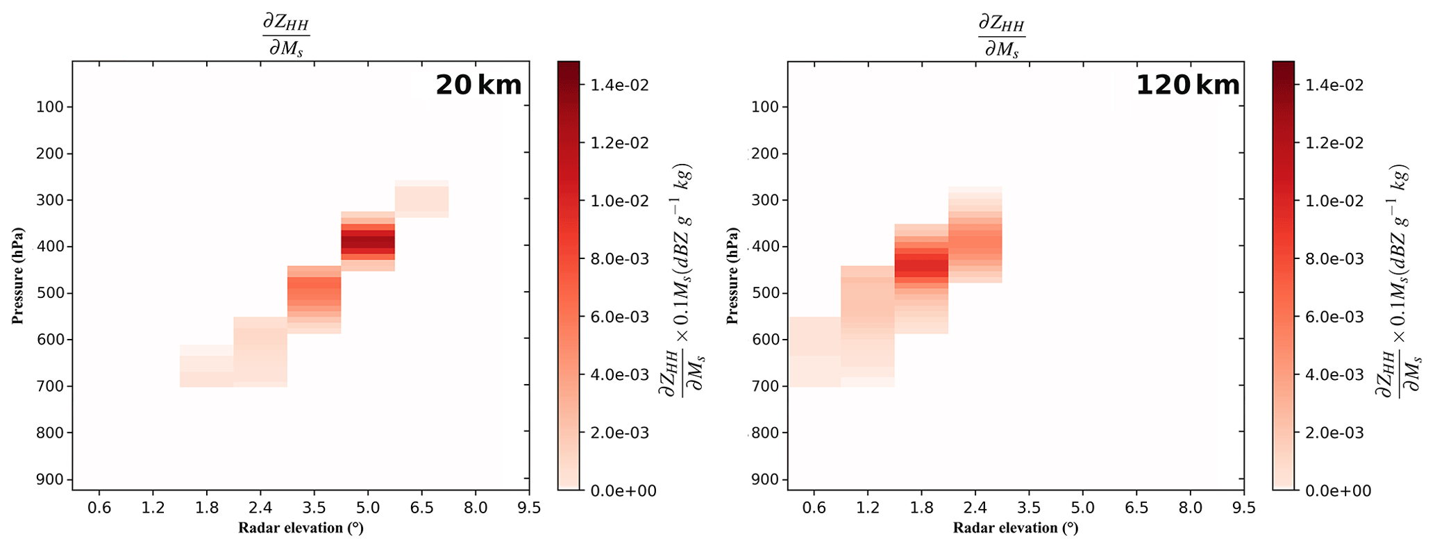
Figure 12ZHH Jacobian for a snow content perturbation associated with the AROME hydrometeor profile shown in Fig. 10, artificially located at (a) 20 km and at (b) 120 km from the radar. The Jacobians are normalized by 10 % of the hydrometeor content.
For KDP, sensitivity is found for rain content perturbations, but the one for solid hydrometeors is negligible (Fig. 10c). Indeed, a rain content perturbation will lead to an increase in the amount of matter crossed by radar pulses and then to a KDP increase. The same results are not obtained for the other hydrometeor contents because of the smaller associated dielectric constant. Concerning ρHV, no sensitivity has been found, except for rain content perturbations in the melting layer.
To conclude this section, it has been found that DPOL variables are more sensitive to rain content perturbations than to other hydrometeors, mainly because of large values of liquid water dielectric constant. Another important information is that the most sensitive DPOL variable appears to be the horizontal reflectivity ZHH, followed by the differential reflectivity ZDR and then by the specific differential phase KDP. The co-polar correlation coefficient ρHV has very small sensitivities to rain content perturbations only. Moreover, since strongly non-Gaussian innovation statistics have been noted in Sect. 3.2, this quantity can be hardly used in data assimilation with the current observation operator and cloud microphysical scheme.
4.3 Jacobian matrix in the observation space
As observations are not available on the model grid, the NL observation operator has to compute the model equivalent in the observation space. To do so, after a horizontal interpolation of the model profiles to the observation location, ℋDPOL computes the DPOL variables on the model profiles and then interpolates them over the main lobe of the radar beam (see Wattrelot et al., 2014). Contrary to Jacobians computed in the model space, the ones obtained in the observation space are represented by a full Jacobian matrix. It has been computed for the four DPOL variables, but only results for ZHH and ZDR are shown and discussed here. Comparable conclusions can be drawn for the other variables.
Figure 11 displays such a complete for the profile displayed in Fig. 10 located at 80 km from the radar. The presence of rain sensitivity between the ground and approximatively 700 hPa is consistent with the hydrometeor content profiles (Fig. 10e). Nevertheless, it can be seen that the values are now split over the two radar elevations which sample rain. Indeed, for a rain content perturbation applied at 800 hPa, for example, the impact on the Jacobian values is noted over the two first radar elevations, with a larger impact on the 0.6∘ elevation. This behavior is explained by the Gaussian shape used to represent the main lobe of the radar beam. In that way, a perturbation applied near of the center of the radar main lobe will have a more important impact on the Jacobian than if applied to its sides.
An interesting feature is also present on the ZDR Jacobians for rain content perturbation. Indeed, ZDR is known to increase when the scanned atmosphere is composed of nonspherical particles. However, the Jacobian values around 700 hPa indicate that a positive rain content perturbation leads to a small decrease in the ZDR value. As rain water content is small, this is actually caused by the addition of very small rain drops. Indeed, as described in Sect. 2.1.1, the hydrometeor content is the variable which influences the particle size distribution through the shape distribution parameter. For small hydrometeor contents, a majority of small particles are regarded as spherical. In consequence, with small rain contents, a positive perturbation will cause the addition of spherical or nearly spherical particles in the scanned volume and then a decrease in the ZDR value.
Another important parameter to consider when dealing with radar geometry is the distance to the radar. With the radar beam being represented as a cone (see Fig. 3 in Wattrelot et al., 2014), the width of the beam and the altitude of the sampled volume are proportional to the distance to the radar. To quantify this effect on the Jacobian values, the convective hydrometeor content profile has been artificially placed at 20 and 120 km from the radar. Figure 12 presents such Jacobians for ZHH with respect to a snow content perturbation. First, no matter the distance to the radar, the positive snow content perturbation leads to an increase in ZHH, related to the increase in the total cross section. Concerning the radar geometry, two effects due to the distance to the radar (beam width and altitude) are observed. The first one is the beam width enlargement. For an elevation of 2.4∘, ZHH sensitivity information lies between about 675 and 550 hPa (Fig. 12a) at 20 km from the radar, while, at 120 km, it lies between 500 and 300 hPa. The side effect of radar beam broadening is a sensitivity reduction due to a repartition of the same amount of information in a larger volume. Indeed, at 20 km, the highest Jacobian value is about 1.4.10−2 dBZ g−1 kg ×0.1Ms (Fig. 12a), while at 120 km, it drops to 8.10−3 dBZ g−1 kg ×0.1Ms (Fig. 12b). The second effect of the radar geometry is related to the altitude. Indeed, the further the observation from the radar is, the higher in the atmosphere it is. This effect is visible in Fig. 12. At 20 km from the radar (Fig. 12a), the elevation angle 5.0∘ is low enough to get information in the snow region. Nevertheless, at 120 km from the radar and with an elevation angle of 5.0∘, the radar beam is located aloft of the snow region.
This paper focused on studying operators required for the variational assimilation of polarimetric variables from ground-based weather radars in convective-scale NWP models. For that purpose, a radar observation operator ℋDPOL, based on the T-matrix theory, was used for the simulation of the following polarimetric variables: horizontal reflectivity ZHH, differential reflectivity ZDR, specific differential phase KDP and co-polar correlation coefficient ρHV. To simulate these variables, ℋDPOL uses hydrometeor contents (rain, snow, graupel and pristine ice) from the AROME-France model. It has been found that more realistic simulations are obtained in the presence of liquid hydrometeors, especially for KDP. To investigate the complexity of DPOL variable simulations, parameters used to characterize hydrometeors in the T-matrix method have been perturbed, such as hydrometeor aspect ratios, dielectric constant or oscillation. A weak sensitivity of the simulations to those parameters has been found, except for the dielectric constants of solid hydrometeors in the case of simulated ZHH and for the rain aspect ratio for ZDR and KDP.
Even if polarimetric radars are able to detect fine spatial structures, filters need to be applied in order to remove non-meteorological data as well as the possible noise. A positive effect of these filters has been found on innovation statistics for the four DPOL variables computed for 12 different meteorological cases, with reductions in biases and standard deviations. Nevertheless, only ZHH and ZDR innovations distributions appear to be close to a Gaussian shape. Innovation distributions as a function of altitude show the complexity of simulations in the presence of solid hydrometeors but also for levels where a melting layer can be encountered.
A linearized version of the polarimetric observation operator has been evaluated by computing its Jacobians with the finite difference method. The results show that polarimetric variables are more sensitive to rain content perturbations than to solid hydrometeor ones, especially because of their different dielectric constants. The Jacobian computation also supports the fact that ZHH appears to be the most sensitive variable to hydrometeor content perturbations, followed by ZDR. Small KDP sensitivity to rain content contents was found, while no sensitivity was detected for ρHV. Then, radar measurement geometry was considered to study DPOL variables sensitivities. Long distances between radar and the profile of interest decrease the sensitivity due to the beam broadening but also induce sensitivities at higher altitudes due to the radar elevation angle.
The present results show that only some DPOL variables appear to be promising for the initialization of hydrometeor contents through variational data assimilation. Among them, the horizontal reflectivity ZHH and the differential reflectivity ZDR are good candidates. The specific differential phase KDP might also be useful for rain. Nevertheless, the simulation of the polarimetric variables for certain types of precipitation or meteorological cases remains difficult. The main reason comes from the ICE3 one-moment microphysical scheme that has been used both in the calibration of the T Matrix and in the AROME-France NWP model from which the simulations have been performed. In this microphysical scheme, the generalized Gamma distributions, used to describe hydrometeor distributions, have shapes which are only driven by the hydrometeor content. DPOL variables being very sensitive to hydrometeor size distributions, such microphysical scheme appears to be limiting. Another limitation is the use of a single particle shape affected by an axis ratio, while DPOL variables are known to be sensitive to hydrometeor shapes. A two-moment microphysical scheme coupled with more complex hydrometeor shapes and scattering computation method such as DDA proposed by DeVoe (1964) could lead to large improvements.
Despite the difficulties encountered for KDP and ρHV simulations, assimilation tests should be run for ZHH and ZDR for all types of hydrometeors, while KDP could be used for rain content initialization only. This will be done in a future study performed in a 1D-Var DA system, in which both nonlinear and linear operators presented here will be exploited. The quantification of errors in ℋDPOL and the study on innovation statistics that have been presented in this paper will also be very useful for characterizing observation errors. Nevertheless, these values constitute first approximations which need to be diagnosed with a more objective method, as the one proposed by Desroziers et al. (2005). In that context, the impact of the DPOL assimilation for analyzing hydrometeor contents as well as temperature and humidity will be studied in this framework.
The polarimetric observation operator is available in the MESO-NH NWP model. It is a non-hydrostatic research model under the CeCILL-C free licence. For more information, please consult the MESO-NH website (http://mesonh.aero.obs-mip.fr/mesonh54, last accesss: 29 April 2020).
The Météo France polarimetric radar data are accessible for a license fee only. For more information, please consult the following web page: https://donneespubliques.meteofrance.fr/?fond=produit&id_produit=105&id_rubrique=35, (last access: 29 April 2020).
All the authors conducted the research and analysis. GT wrote the paper. All the authors contributed to the paper's improvement.
The authors declare that they have no conflict of interest.
This research was conducted during the Guillaume Thomas' PhD, funded by Météo France. The authors would like to thank Sylvain Chaumont for providing polarimetric radar data. In addition, the authors also want to thank Nan Yu and Béatrice Fradon for their advice and their carefulness about those data, and Eric Wattrelot for much advice given during the first year of this PhD. Special acknowledgements are also due to Maud Martet, who helped with the polarimetric data decoding, provided advice on weather radar technology and agreed to provide an internal review of this paper. Finally, the authors would like to thank Isaac Moradi, who agreed to edit this paper, as well as the two anonymous referees, who helped to improve the present paper.
This paper was edited by Isaac Moradi and reviewed by two anonymous referees.
Al-Sakka, H., Boumahmoud, A.-A., Fradon, B., Frasier, S. J., and Tabary, P.: A New Fuzzy Logic Hydrometeor Classification Scheme Applied to the French X-, C-, and S-Band Polarimetric Radars, J. Appl. Meteorol. Clim., 52, 2328–2344, https://doi.org/10.1175/jamc-d-12-0236.1, 2013. a
Augros, C., Caumont, O., Ducrocq, V., Gaussiat, N., and Tabary, P.: Comparisons between S-, C- and X-band polarimetric radar observations and convective-scale simulations of the HyMeX first special observing period, Q. J. Roy. Meteor. Soc., 142, 347–362, https://doi.org/10.1002/qj.2572, 2015. a, b, c, d, e
Benjamin, S. G., Weygandt, S. S., Brown, J. M., Hu, M., Alexander, C. R., Smirnova, T. G., Olson, J. B., James, E. P., Dowell, D. C., Grell, G. A., Lin, H., Peckham, S. E., Smith, T. L., Moninger, W. R., Kenyon, J. S., and Manikin, G. S.: A North American Hourly Assimilation and Model Forecast Cycle: The Rapid Refresh, Mon. Weather Rev., 144, 1669–1694, https://doi.org/10.1175/mwr-d-15-0242.1, 2016. a
Bick, T., Simmer, C., Trömel, S., Wapler, K., Franssen, H.-J. H., Stephan, K., Blahak, U., Schraff, C., Reich, H., Zeng, Y., and Potthast, R.: Assimilation of 3D radar reflectivities with an ensemble Kalman filter on the convective scale, Q. J. Roy. Meteor. Soc., 142, 1490–1504, https://doi.org/10.1002/qj.2751, 2016. a
Brandes, E. A., Zhang, G., and Vivekanandan, J.: Experiments in Rainfall Estimation with a Polarimetric Radar in a Subtropical Environment, J. Appl. Meteorol., 41, 674–685, https://doi.org/10.1175/1520-0450(2002)041<0674:eirewa>2.0.co;2, 2002. a
Bringi, V. N., Rasmussen, R. M., and Vivekanandan, J.: Multiparameter Radar Measurements in Colorado Convective Storms. Part I: Graupel Melting Studies, J. Atmos. Sci., 43, 2545–2563, https://doi.org/10.1175/1520-0469(1986)043<2545:mrmicc>2.0.co;2, 1986. a
Brousseau, P., Seity, Y., Ricard, D., and Léger, J.: Improvement of the forecast of convective activity from the AROME-France system, Q. J. Roy. Meteor. Soc., 142, 2231–2243, https://doi.org/10.1002/qj.2822, 2016. a, b
Caniaux, G., Redelsperger, J.-L., and Lafore, J.-P.: A Numerical Study of the Stratiform Region of a Fast-Moving Squall Line. Part I: General Description and Water and Heat Budgets, J. Atmos. Sci., 51, 2046–2074, https://doi.org/10.1175/1520-0469(1994)051<2046:ansots>2.0.co;2, 1994. a
Caumont, O., Ducrocq, V., Delrieu, G., Gosset, M., Pinty, J.-P., Parent du Chatelet, J., Andrieu, H., Lemaitre, Y., and Scialom, G.: A Radar Simulator for High-Resolution Nonhydrostatic Models, J. Atmos. Ocean. Tech., 23, 1049–1067, https://doi.org/10.1175/JTECH1905.1, 2006. a, b, c, d
Caumont, O., Ducrocq, V., Wattrelot, E., Jaubert, G., and Pradier-Vabre, S.: 1D+3DVar assimilation of radar reflectivity data: a proof of concept, Tellus A, 62, 173–187, https://doi.org/10.1111/j.1600-0870.2009.00430.x, 2010. a
Desroziers, G., Berre, L., Chapnik, B., and Poli, P.: Diagnosis of observation, background and analysis-error statistics in observation space, Q. J. Roy. Meteor. Soc., 131, 3385–3396, https://doi.org/10.1256/qj.05.108, 2005. a
Dowell, D. C., Wicker, L. J., and Snyder, C.: Ensemble Kalman Filter Assimilation of Radar Observations of the 8 May 2003 Oklahoma City Supercell: Influences of Reflectivity Observations on Storm-Scale Analyses, Mon. Weather Rev., 139, 272–294, https://doi.org/10.1175/2010mwr3438.1, 2011. a
Ducrocq, V., Ricard, D., Lafore, J.-P., and Orain, F.: Storm-Scale Numerical Rainfall Prediction for Five Precipitating Events over France: On the Importance of the Initial Humidity Field, Weather Forecast., 17, 1236–1256, https://doi.org/10.1175/1520-0434(2002)017<1236:ssnrpf>2.0.co;2, 2002. a
Duerinckx, A., Hamdi, R., Mahfouf, J.-F., and Termonia, P.: Study of the Jacobian of an extended Kalman filter for soil analysis in SURFEXv5, Geosci. Model Dev., 8, 845–863, https://doi.org/10.5194/gmd-8-845-2015, 2015. a
Errico, R. M., Fillion, L., Nychka, D., and Lu, Z.-Q.: Some statistical considerations associated with the data assimilation of precipitation observations, Q. J. Roy. Meteor. Soc., 126, 339–359, https://doi.org/10.1002/qj.49712656217, 2000. a
Errico, R. M., Bauer, P., and Mahfouf, J.-F.: Issues Regarding the Assimilation of Cloud and Precipitation Data, J. Atmos. Sci., 64, 3785–3798, https://doi.org/10.1175/2006jas2044.1, 2007. a
Gao, J. and Stensrud, D. J.: Assimilation of Reflectivity Data in a Convective-Scale, Cycled 3DVAR Framework with Hydrometeor Classification, J. Atmos. Sci., 69, 1054–1065, https://doi.org/10.1175/JAS-D-11-0162.1, 2011. a
Gourley, J. J., Tabary, P., and du Chatelet, J. P.: A Fuzzy Logic Algorithm for the Separation of Precipitating from Nonprecipitating Echoes Using Polarimetric Radar Observations, J. Atmos. Ocean. Tech., 24, 1439–1451, https://doi.org/10.1175/jtech2035.1, 2007. a, b
Gustafsson, N., Janjić, T., Schraff, C., Leuenberger, D., Weissmann, M., Reich, H., Brousseau, P., Montmerle, T., Wattrelot, E., Bučánek, A., Mile, M., Hamdi, R., Lindskog, M., Barkmeijer, J., Dahlbom, M., Macpherson, B., Ballard, S., Inverarity, G., Carley, J., Alexander, C., Dowell, D., Liu, S., Ikuta, Y., and Fujita, T.: Survey of data assimilation methods for convective-scale numerical weather prediction at operational centres, Q. J. Roy. Meteor. Soc., 144, 1218–1256, https://doi.org/10.1002/qj.3179, 2018. a, b, c
Ikuta, Y. and Honda, Y.: Development of 1D+4DVAR data assimilation of radar reflectivity in JNoVA, CAS/JSC WGNE Res. Activ. Atmos. Oceanic Model., 41, 2011. a
Jung, Y., Zhang, G., and Xue, M.: Assimilation of Simulated Polarimetric Radar Data for a Convective Storm Using the Ensemble Kalman Filter. Part I: Observation Operators for Reflectivity and Polarimetric Variables, Mon. Weather Rev., 136, 2228–2245, https://doi.org/10.1175/2007mwr2083.1, 2008. a
Kumjian, M.: Principles and applications of dual-polarization weather radar. Part I: Description of the polarimetric radar variables, Journal of Operational Meteorology, 1, 226–242, https://doi.org/10.15191/nwajom.2013.0119, 2013a. a, b
Kumjian, M.: Principles and applications of dual-polarization weather radar. Part II: Warm- and cold-season applications, Journal of Operational Meteorology, 1, 243–264, https://doi.org/10.15191/nwajom.2013.0120, 2013b. a
Liu, G.: A Database of Microwave Single-Scattering Properties for Nonspherical Ice Particles, B. Am. Meteorol. Soc., 89, 1563–1570, https://doi.org/10.1175/2008bams2486.1, 2008. a
Llasat, M. C., Llasat-Botija, M., Prat, M. A., Porcú, F., Price, C., Mugnai, A., Lagouvardos, K., Kotroni, V., Katsanos, D., Michaelides, S., Yair, Y., Savvidou, K., and Nicolaides, K.: High-impact floods and flash floods in Mediterranean countries: the FLASH preliminary database, Adv. Geosci., 23, 47–55, https://doi.org/10.5194/adgeo-23-47-2010, 2010. a
Matrosov, S.: Assessment of Radar Signal Attenuation Caused by the Melting Hydrometeor Layer, IEEE T. Geosci. Remote, 46, 1039–1047, https://doi.org/10.1109/tgrs.2008.915757, 2008. a
Mishchenko, M. I. and Travis, L. D.: T-matrix computations of light scattering by large spheroidal particles, Opt. Commun., 109, 16–21, https://doi.org/10.1016/0030-4018(94)90731-5, 1994. a
Montmerle, T. and Faccani, C.: Mesoscale Assimilation of Radial Velocities from Doppler Radars in a Preoperational Framework, Mon. Weather Rev., 137, 1939–1953, https://doi.org/10.1175/2008mwr2725.1, 2009. a
Pinty, J. and Jabouille, P.: A mixed-phase cloud parameterization for use in mesoscale non-hydrostatic model: simulations of a squall line and of orographic precipitations, in: Conf. on Cloud Physics, American Meteorological Society Everett, WA, 217–220, 1998. a
Ridal, M. and Dahlbom, M.: Assimilation of Multinational Radar Reflectivity Data in a Mesoscale Model: A Proof of Concept, J. Appl. Meteorol. Clim., 56, 1739–1751, https://doi.org/10.1175/jamc-d-16-0247.1, 2017. a
Ryzhkov, A., Pinsky, M., Pokrovsky, A., and Khain, A.: Polarimetric Radar Observation Operator for a Cloud Model with Spectral Microphysics, J. Appl. Meteorol. Clim., 50, 873–894, https://doi.org/10.1175/2010jamc2363.1, 2011. a, b, c
Ryzhkov, A. V., Schuur, T. J., Burgess, D. W., Heinselman, P. L., Giangrande, S. E., and Zrnic, D. S.: The Joint Polarization Experiment: Polarimetric Rainfall Measurements and Hydrometeor Classification, B. Am. Meteorol. Soc., 86, 809–824, https://doi.org/10.1175/bams-86-6-809, 2005. a
Seity, Y., Brousseau, P., Malardel, S., Hello, G., Bénard, P., Bouttier, F., Lac, C., and Masson, V.: The AROME-France convective scale operational model, Mon. Weather Rev., 139, 976–991, https://doi.org/10.1175/2010MWR3425.1, 2011. a
Seliga, T. A. and Bringi, V. N.: Potential Use of Radar Differential Reflectivity Measurements at Orthogonal Polarizations for Measuring Precipitation, J. Appl. Meteorol., 15, 69–76, https://doi.org/10.1175/1520-0450(1976)015<0069:puordr>2.0.co;2, 1976. a
Sun, J.: Convective-scale assimilation of radar data: Progress and challenges, Q. J. Roy. Meteor. Soc., 131, 3439–3463, https://doi.org/10.1256/qj.05.149, 2005. a
Sun, J. and Crook, N.: Dynamical and Microphysical Retrieval from Doppler Radar Observations Using a Cloud Model and Its Adjoint. Part I: Model Development and Simulated Data Experiments, J. Atmos. Sci., 54, 1642–1661, 1997. a
Sun, J. and Wang, H.: Radar Data Assimilation with WRF 4D-Var. Part II: Comparison with 3D-Var for a Squall Line over the U.S. Great Plains, Mon. Weather Rev., 141, 2245–2264, https://doi.org/10.1175/mwr-d-12-00169.1, 2013. a
Tabary, P.: The New French Operational Radar Rainfall Product. Part I: Methodology, Weather Forecast., 22, 393–408, https://doi.org/10.1175/waf1004.1, 2007. a, b
Tabary, P., Fradon, B., and Boumahmoud, A.-A.: La polarimétrie radar à Météo-France, La Météorologie, 8, 59–67, https://doi.org/10.4267/2042/52055, 2013. a
Tong, M. and Xue, M.: Ensemble Kalman Filter Assimilation of Doppler Radar Data with a Compressible Nonhydrostatic Model: OSS Experiments, Mon. Weather Rev., 133, 1789–1807, https://doi.org/10.1175/mwr2898.1, 2005. a
Wang, H., Sun, J., Fan, S., and Huang, X.-Y.: Indirect Assimilation of Radar Reflectivity with WRF 3D-Var and Its Impact on Prediction of Four Summertime Convective Events, J. Appl. Meteorol. Clim., 52, 889–902, https://doi.org/10.1175/jamc-d-12-0120.1, 2013a. a
Wang, H., Sun, J., Zhang, X., Huang, X.-Y., and Auligné, T.: Radar Data Assimilation with WRF 4D-Var. Part I: System Development and Preliminary Testing, Mon. Weather Rev., 141, 2224–2244, https://doi.org/10.1175/mwr-d-12-00168.1, 2013b. a
Waterman, P.: Matrix formulation of electromagnetic scattering, P. IEEE, 53, 805–812, https://doi.org/10.1109/proc.1965.4058, 1965. a
Wattrelot, E., Caumont, O., and Mahfouf, J.-F.: Operational Implementation of the 1D+3D-Var Assimilation Method of Radar Reflectivity Data in the AROME Model, Mon. Weather Rev., 142, 1852–1873, https://doi.org/10.1175/mwr-d-13-00230.1, 2014. a, b, c, d
The reader should note that “horizontal reflectivity” (ZHH) in this paper relates to the horizontal equivalent reflectivity.
The Jacobian study has been done with linear reflectivity units in order to stay closer to a linear regime than would be possible with the use of logarithmic reflectivity units.