the Creative Commons Attribution 4.0 License.
the Creative Commons Attribution 4.0 License.
 | 20 Jan 2020
The polarized Sun and sky radiometer SSARA: design, calibration, and application for ground-based aerosol remote sensing
Claudia Emde
Matthias Wiegner
Meinhard Seefeldner
Linda Forster
Bernhard Mayer
Recently, polarimetry has been used to enhance classical photometry to infer aerosol optical properties, as polarized radiation contains additional information about the particles. Therefore, we have equipped the Sun–sky automatic radiometer (SSARA) with polarizer filters to measure linearly polarized light at 501.5 nm.
We describe an improved radiometric and polarimetric calibration method, which allows us to simultaneously determine the linear polarizers' diattenuation and relative orientation with high accuracy (0.002 and 0.1∘, respectively). Furthermore, we employed a new calibration method for the alt-azimuthal mount capable of correcting the instrument's pointing to within 32 arcmin. So far, this is limited by the accuracy of the Sun tracker. Both these methods are applicable to other Sun and sky radiometers, such as the Cimel CE318-DP instruments used in the AErosol RObotic NETwork (AERONET).
During the A-LIFE (Absorbing aerosol layers in a changing climate: aging, LIFEtime and dynamics) field campaign in April 2017, SSARA collected 22 d of data. Here, we present two case studies. The first demonstrates the performance of an aerosol retrieval from SSARA observations under partially cloudy conditions. In the other case, a high aerosol load due to a Saharan dust layer was present during otherwise clear-sky conditions.
- Article
(9155 KB) - Full-text XML
- BibTeX
- EndNote


According to the Intergovernmental Panel on Climate Change (IPCC), aerosols have a significant and not entirely understood impact on the Earth's climate (IPCC, 2013). In the first order, it induces a direct radiative forcing effect. Additionally, it has been established that aerosols have an influence on the development and lifetime of clouds (Albrecht, 1989), which is known as the secondary aerosol effect. In order to study these effects, aerosol properties have to be retrieved in the vicinity of clouds. To gain insight into processes occurring on or close to the edge of clouds, microphysical properties of the aerosol are required in addition to the total aerosol load, quantified by the aerosol optical depth (AOD). These are, for instance, information about the size distribution of the particles, their index of refraction, and single scattering albedo (related to the absorptance). The combination of these parameters can be used to identify the chemical composition, and, eventually, source region of the aerosol. This has, in turn, impact on the aerosol's hygroscopicity and therefore the microphysical properties of the cloud droplets that might develop from it.
Aerosols can be measured from satellites and from the ground. While the former has the advantage of global coverage, a spatial resolution on the order of 100 m would be required to properly resolve smaller clouds and the aerosol in between them, which is not the case for most satellite products. Ground-based systems are better suited for these studies, e.g., the AErosol RObotic NETwork (AERONET) that has been established as a large network of ground-based Sun photometers (Holben et al., 1998; Giles et al., 2019).
Classically, aerosol microphysical properties are retrieved from multispectral measurements. Recently, polarimetric measurements started to be included as well. Several studies suggest that including polarimetric information in retrievals yields additional information on the aerosol. Xu and Wang (2015) investigated the gain in information content from adding polarized measurements to principal plane and almucantar scans. In a later paper, they applied their retrieval to real-world AERONET measurements (Xu et al., 2015). The retrieval error was significantly reduced for size distribution parameters (50 %), refractive index (10 %–30 %), and single scattering albedo (10 %–40 %). Dubovik et al. (2006) suggest that polarimetric measurements can be used to gain more insight into the aerosol particle shape. This was further examined by Fedarenka et al. (2016), ascertaining an improvement in retrieval stability for fine-mode-dominated aerosols, and a high sensitivity to particle shape, due to the use of polarimetry.
Predating these efforts was the POLDER instrument aboard the PARASOL satellite (Deschamps et al., 1994), measuring polarized reflectance. Its data have been used for aerosol retrievals (Hasekamp and Landgraf, 2007; Hasekamp et al., 2011). More recently, the Spectropolarimeter for Planetary EXploration (SPEX) has been developed (van Harten et al., 2011). Originally designed as a satellite instrument (van Amerongen et al., 2017), a ground-based version has been built (van Harten et al., 2014). Both of them have been used for retrieving aerosol properties (Di Noia et al., 2015). Equivalently, GroundMSPI (Diner et al., 2012) is the ground-based version of the Multiangle SpectroPolarimetric Imager (MSPI).
Polarimetric instruments require an additional calibration. Prior work on this has been done for polarized Cimel CE318-DP Sun photometers by Li et al. (2010, 2014, 2018). In this paper, we present an alternative approach that overcomes some of their limitations and reduces the number of required steps by simultaneously determining the polarizers' efficiencies and angles.
Our new methodology was applied to polarized radiance measurements from the polarized Sun–sky automatic radiometer (SSARA), taken during the A-LIFE (Absorbing aerosol layers in a changing climate: aging, LIFEtime and dynamics) field campaign. It took place in Cyprus during April 2017 and included ground-based components, such as lidar and radar systems, radiometers, and in situ samplers at Paphos and Limassol. Additionally, a research aircraft with in situ instrumentation was operated from Paphos airport. The goal of the A-LIFE project is to investigate the effects of aerosol on the Earth's radiation budget, cloud development, and atmospheric dynamics, with a focus on absorbing aerosols, such as black carbon and desert dust. SSARA was previously employed in the SAMUM-1 and 2, and the SALTRACE field campaigns that had similar goals (Toledano et al., 2009, 2011).
This paper consists of two parts. Section 2 first characterizes the SSARA instrument. Then, it describes the calibration methods for the instrument and the alt-azimuthal mount. The second part in Sect. 3 introduces the aerosol retrieval and then presents the findings for two case studies from the A-LIFE campaign. Section 4 summarizes the findings and gives an outlook for further studies. Additionally, a short primer in quaternion algebra is included in Appendix A.
2.1 Instrument characterization
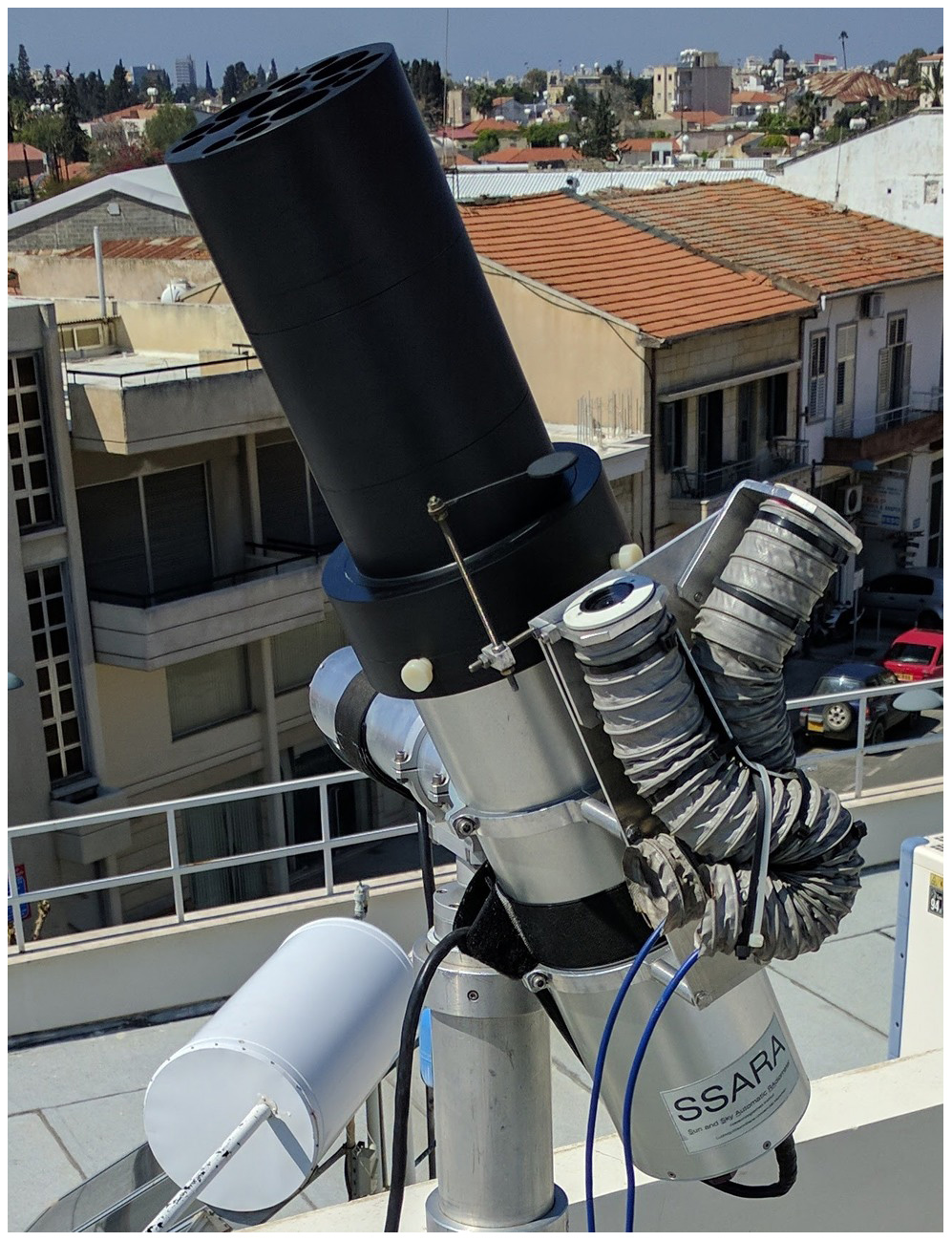
SSARA is a multispectral Sun photometer that has been designed and built at the Meteorological Institute Munich (Wagner et al., 2003). The instrument consists of three main components. These are the sensor head, an alt-azimuthal mount, and a controller box containing a programmable logic controller (PLC). The latter is responsible for actuating the mount, operating the sensor head with all its life support, and digitizing the sensor head's signals.
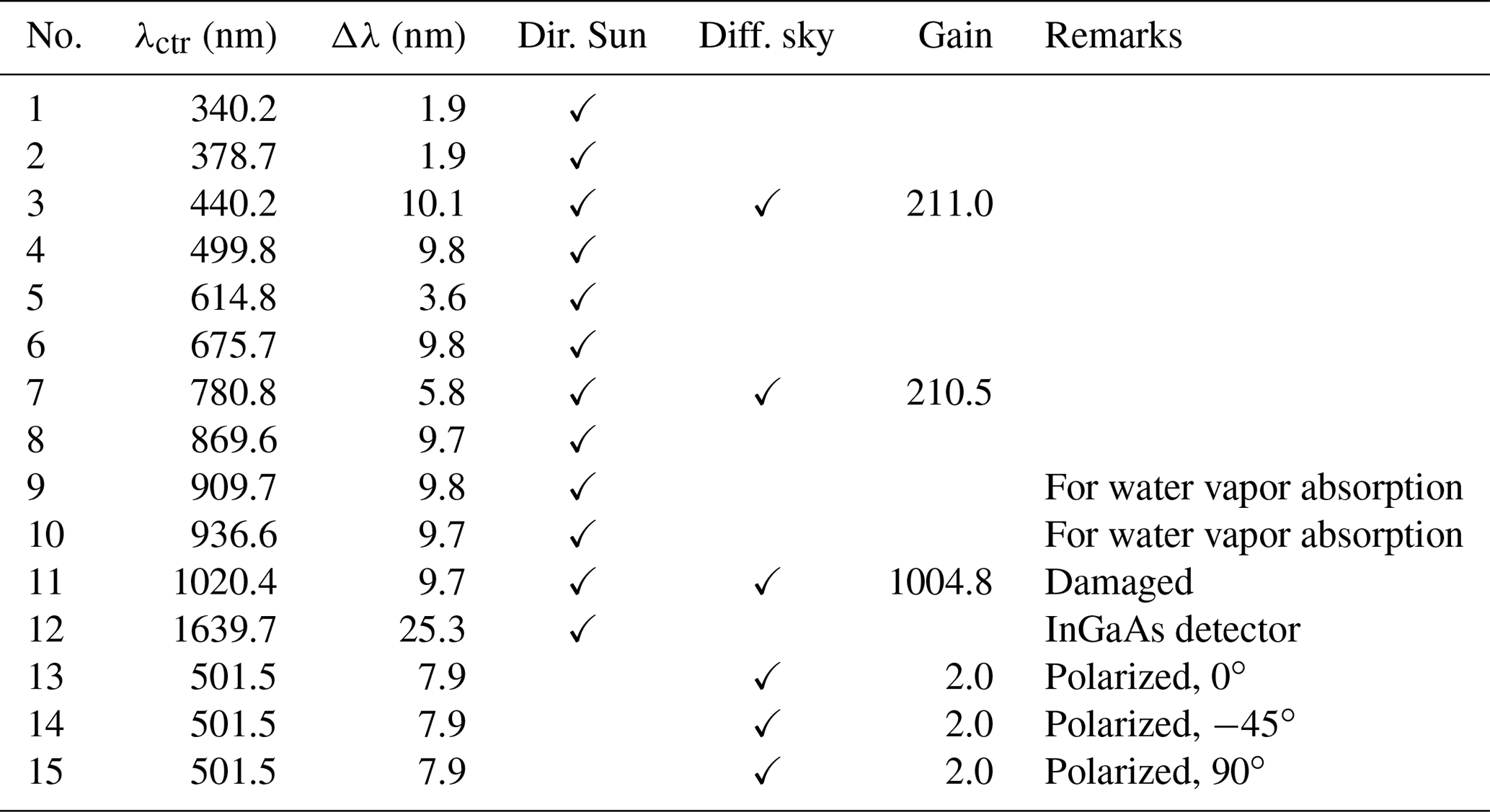
The radiometer's sensor head (Fig. 1) houses baffles for 15 channels. The selection of wavelengths for the channels is done by bandpass interference filters in front of the baffles. Their characteristics are given in Table 1. All channels are installed parallel to each other, allowing for simultaneous measurements at different wavelengths and polarizations. This is a big advantage, in particular for aerosol observations during cloudy conditions with high temporal variability. The pointing of the channels is parallel to within 20 arcmin.
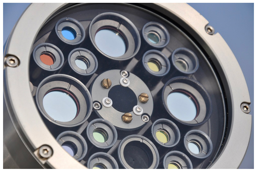
Figure 1SSARA sensor head with 12 direct channels (smaller diameter tubes) and three polarized channels (larger diameter at the top, left, and right). The quadrant Sun tracker is in the center; below it is a finder for manual Sun tracking.
Channels 1–12 are designed for Sun radiance measurements. They are set up as pinhole optics to avoid an image of the Sun on the detectors. At these channels, the field of view (FOV) of the center point of the detectors is 1.2∘ full cone. This FOV, and also the wavelength, bandwidth, and out-of-band blocking of the interference filters, has been chosen to be similar to Cimel Sun photometers used in AERONET. The remaining three channels (13–15) are designed for sky radiance measurements and are set up as lens optics to obtain a larger, i.e., 11 times larger, aperture than that of channels 1–12. Their FOV is also 1.2∘ full cone. In addition to the bandpass interference filters, channels 13–15 were recently equipped with linear polarizers. These are made from linear film polarizer sheets and are oriented at roughly 0, −45, and 90∘ relative to the sensor head's horizontal axis. Channels 3, 7, and 11, as well as channels 13–15 are equipped with a second amplifier stage to increase their dynamic range. This allows for measurements of the sky radiance, which is several orders of magnitude smaller than the direct Sun radiance. These measurements are performed in the solar principal and the almucantar plane. Furthermore, the sensor head includes a four-quadrant sensor for tracking the Sun.
The instrument can perform measurements at a maximum time resolution of about 1.6 s, which is used for the direct measurements. Due to the design of the electronics, the amplifiers of the polarized channels have a higher time constant of 1 s (compared to 0.25 s in the direct channels). For scans, we therefore wait 6 s to allow for the detector signal to settle, preventing the measurements at different scanning angles from “blurring” into one another.
Table 1SSARA channel configuration from 23 January 2017 onward. λctr is the central wavelength of the filter; Δλ is its full width at half maximum. “Gain” gives the amplification of the second amplifier stage if installed for the corresponding channel. The “dir. Sun” and “diff. sky” columns indicate whether the channel can be used for direct Sun or diffuse sky radiance measurements, respectively. InGaAs refers to indium gallium arsenide.
The sensor head is mounted on a two-axis alt-azimuthal mount (Seefeldner et al., 2004). Its stepper motors have a resolution of 0.009∘ (32.4 arcsec). In order to apply proper corrections to the Rayleigh scattering background, the air pressure is recorded as well. The sensor head is continuously heated to 40 ∘C to minimize drifts in sensor and filter characteristics.
Sunlight scattered from the glass window and possible dirt particles on it can create straylight, especially at larger scattering angles. To minimize this effect, a baffle has been designed and built in preparation of the A-LIFE campaign. It consists of a 24 cm long, black PVC cylinder with openings for the channels, leaving a 2 mm clearing to their FOV. Figure 2 shows how the straylight baffle is mounted. This should inhibit direct sunlight from hitting the front glass for scattering angles greater than 3.5∘.
The scan patterns and wavelengths of SSARA are similar to those of the Cimel instruments used in AERONET, allowing for comparison. However, in contrast to Cimel, it is able to measure all its channels simultaneously, because it does not use a filter wheel. For Cimel, the filter wheel sequence takes several seconds, limiting its time resolution. Also, since it is not part of an operational network, it can be operated in any mode deemed appropriate. For instance, sky radiance scans can be performed at a higher rate or even using new patterns for testing.
2.2 Calibration
2.2.1 Polarimetric calibration
Polarized radiation can be described by what is known as the “Stokes vector” S (Chandrasekhar, 1950). It describes its total intensity, as well as its polarization state.
where Ex and Ey are the strength of the electromagnetic radiation in the two transversal directions. δ is the phase shift between these two components. I describes the total intensity, Q and U the intensity of the linear polarized contribution, and V that of circular polarization. As a result, the first component has to be larger than or equal to the sum of the others. In atmospheric radiative transfer, the contribution of circular polarization is about 3 orders of magnitude smaller compared to linear polarization (e.g., de Haan et al., 1987; Emde et al., 2015, 2018), so it can be ignored here (V≈0). This leads to the definition of the degree of linear polarization (DoLP) η:
The polarimetric and radiometric calibration of the sky radiance channels were recently performed at Laboratoire d'Optique Atmosphérique (LOA) in Lille, France. To produce linear polarized light, a combination of an Ulbricht sphere and the so-called POLBOX was used (Balois, 1998). Figure 3 depicts the calibration setup (see also Li et al., 2018).
The POLBOX acts as a linear polarizer for the unpolarized light coming from the sphere. It consists of two glass plates that can be tilted up to 65∘ relative to the optical axis. According to the Fresnel equations, the total attenuation exerted by a glass plate differs for radiation polarized in the incident plane (I∥) and perpendicular to it (I⟂). Therefore, the DoLP η of the transmitted light is higher than that of the incident light. This degree of linear polarization hereby depends on to the tilting angle of the glass plate α. The Ulbricht sphere used here does not have to be radiometrically calibrated, but its intensity needs to be constant over the time of the calibration.
The output DoLP of the POLBOX can be determined with a high accuracy, as the plate angle can be set with high precision. Li et al. (2010) gives an uncertainty in the DoLP of ∼0.0015; Li et al. (2018) even gives 0.00128. The entire assembly can be rotated around its optical axis, therefore changing the polarization plane of the transmitted light. When using two plates and tilting the second by the same angle α but in the opposite direction, a divergent ray of light hitting the first plate at angle α+δα will hit the second plate at an angle α−δα. This compensates for linear terms of error in the DoLP due to divergent light. It can be shown that the DoLP after the second plate ηtot is given by
Here, α is the angle between the incident light and the normal of the glass plate; α′ is the same but for the refracted light inside the glass. α′ can be calculated using the Snellius law.
The refractive index of air is assumed to be 1. The plates are fabricated from Schott SF-11-type glass. Its data sheet provides coefficients for the Sellmeier equation (Eq. 10), to calculate the refractive index n:
with
The POLBOX has a maximum tilt angle of . The resulting DoLP is roughly 58 % at the SSARA polarized wavelength of 501.5 nm.
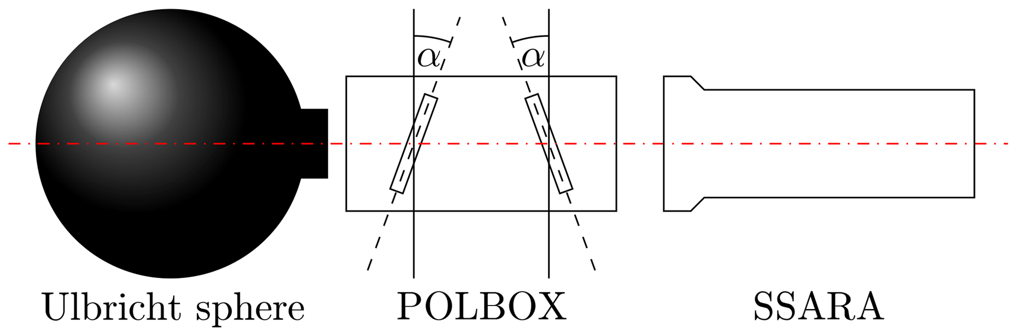
Figure 3Polarimetric calibration setup. The distance between the Ulbricht sphere and the POLBOX, and between the POLBOX and the SSARA sensor head are on the order of a few centimeters along the optical axis (shown as a dashed red line). The glass plate angle α of the POLBOX can be adjusted between 0 and 65∘. Additionally, it can be rotated through 360∘ around the optical axis by the angle ϑ.
In the Stokes–Müller formalism, interactions with optical components or the atmosphere are described by left multiplication of the Stokes vector of the incoming radiation Sin with the appropriate real 4×4 Müller matrices (M1 to Mn):
In this context, a linear polarizer can be described as a linear diattenuator, meaning its attenuation differs for the two directions of polarization. The Müller matrix LD for a linear diattenuator rotated by an arbitrary angle ϑ is given in Bass et al. (2010) as
with , , and . k0 and k1 are the intensity transmission values for the filter in the directions parallel and perpendicular to its orientation, respectively. ϑ is the angle between the polarization direction of the incoming radiation and the filter. Since a photodiode can only measure the total intensity of the light (first component of Stokes vector), the measurement operator 〈M| projects only the first row of the matrix. Mathematically, it can be described as a transposed vector :
The light entering the instrument behind the POLBOX is taken to be polarized only in the positive Q direction. This means the Stokes vector is given by , with ηtot again being the degree of linear polarization produced by the POLBOX. Also, the sensor has a certain radiometric response C, so the measurement vector becomes .
It can be seen that the polarimetric (described by a and b) and radiometric response (C) of the instrument–filter combination cannot be determined separately. Therefore, we introduce and . Also, since the total intensity of the incoming light is unknown, we define and . Measuring the signal S at varying rotation angles ϑ of the POLBOX, the parameters A′, B′ and ϑ0 can be obtained by performing a Levenberg–Marquardt (LM) fit using Eq. (17) as a model. k0 and k1 cannot be determined independently, but it is possible to derive the diattenuation D as
It is independent of the intensity of the incoming radiation (I0), as long as it is stable over the time of the calibration. The LM fit also gives estimations for the uncertainties in A′, B′, and ϑ0. For determining the response a′, we use LOA's SphereX, a radiometrically calibrated Ulbricht sphere. As it provides unpolarized light with known intensity, the measured signal is given by
For the SSARA calibration on 2 February 2017, the fit of Eq. (17) to the measurements can be seen in Fig. 4. The determined values and their uncertainties are shown in Table 2. It should be noted that the sensor head was placed on its right side, therefore adding roughly 90∘ to the filter orientation.
What remains after this calibration is the collective rotation of all channels in the sensor head, which also includes rotations stemming from the mount. When only the degree of linear polarization is of interest, this is not relevant. However, this global rotation has to be known to determine the polarization angle, which influences how the polarized radiation is divided between the Q and U components. As outlined in Li et al. (2014), this could be done by using known features of the Rayleigh background (e.g., U=0 in the principal plane).
Even unpolarized channels can have a polarization sensitivity. However, channels 3, 7, and 11 are assumed to have no polarization dependence, meaning the filters fully transmit light regardless of the polarization state. In future calibration sessions, the validity of this assumption could be investigated.
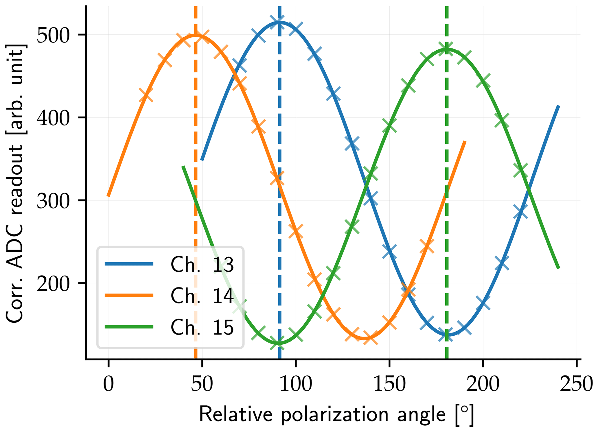
Figure 4Fit of Eq. (17) to intensity measurements of the three polarized SSARA channels at varying POLBOX orientations. The dashed horizontal lines correspond to the angles of maximum transmission ϑ0. Amplitude and vertical offset are related to the radiometric and polarimetric responses.
Table 2Calibration results for measurements on 2 February 2017. The uncertainties are determined from the fit.
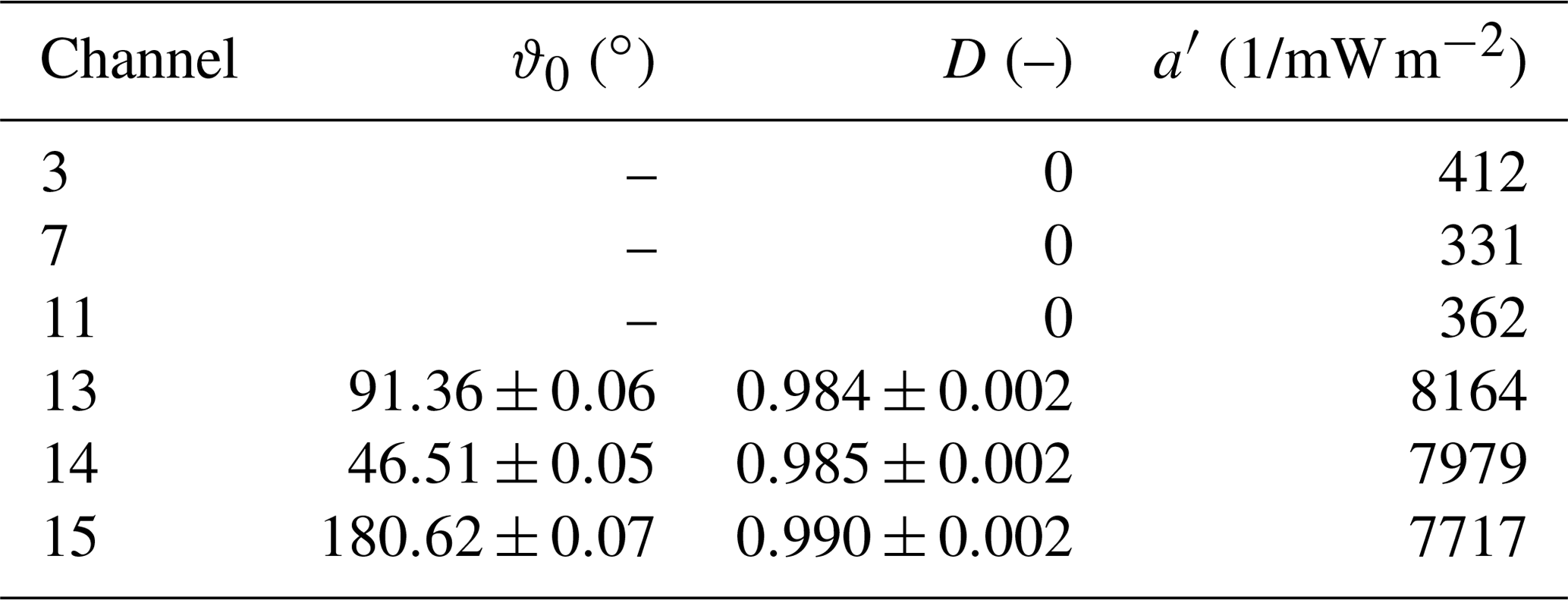
Channels 3, 7, and 11 are assumed to be unpolarized, so , and therefore D=0.
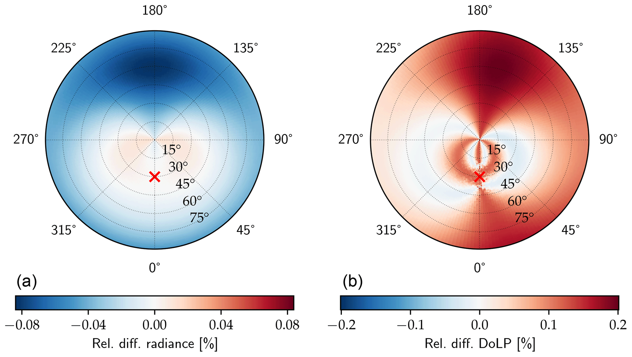
To determine the potential error arising from neglecting the imperfections of the filters and their orientation, a polarized radiance all-sky panorama was simulated for 500 nm using the MYSTIC 3-D Monte Carlo solver (Mayer, 2009; Emde et al., 2010) of the libRadtran package (Mayer and Kylling, 2005; Emde et al., 2016). To get the maximum error corresponding to the highest possible degree of linear polarization, a pure Rayleigh atmosphere was used as model input, without aerosol or clouds. Scattering processes by these would “destroy” polarization. The ground is non-reflective for the same reason, and the Sun is at a zenith angle of 30∘. The simulation is used to generate synthetic measurements in the three polarized SSARA channels, taking into account the filter characteristics from Table 2. From these, the Stokes vector is reconstructed, once assuming perfect polarizers (D=1) at exact angles (90, 45, and 180∘) and again with the actual filter characteristics in Table 2. Their relative difference in the total radiance and the degree of linear polarization is displayed in Figs. 5 and 6, respectively. The relative error in total radiance varies between −1.1 % and +0.8 %, and the relative error in DoLP varies between −2.4 % and +1.5 % (relative, not in absolute value). Due to the relative rotation of the polarizers, the pattern is not symmetrical. To evaluate the remaining difference induced by the uncertainties in ϑ and D shown in Table 2, the rotation angle and diattenuation of the channel 15 polarizer are perturbed by 0.07∘ and 0.002, for Figs. 7 and 8, respectively. For the total radiance, the remaining relative error is below 0.1 %; for the DoLP, it is 0.2 %, so about a factor of 10 smaller than without the calibration.
As mentioned before, POLBOX has an uncertainty of between 0.0015 and 0.00128 in DoLP. Simple Gaussian error propagation can be used to determine the resulting uncertainties in the calibration. Our calibration fits measurements to Eq. (17), where the DoLP produced by the POLBOX is represented by η. As it only affects the amplitude of the cosine, the uncertainty of η propagates to the retrieved value of B′, and, according to Eq. (18), in turn to D. At an assumed DoLP of ∼0.58, an absolute uncertainty of 0.0015 corresponds to a relative uncertainty of 0.26 %. For the D values given in Table 2, this leads to an absolute uncertainty of about 0.0025. This is on the same scale as the uncertainties we determined from the fit. Therefore, it can be assumed that higher accuracy can only be achieved using a light source with a better known DoLP.
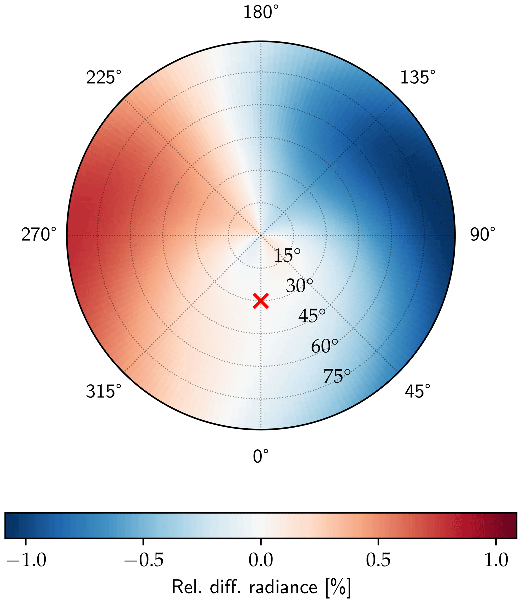
Figure 5Relative difference in measured total radiance at 500 nm due to incorrect rotation and imperfect polarizer for a synthetic scene. The Sun (red marker) is at a zenith angle of 30∘ and azimuth 0∘.

Figure 6Same as Fig. 5 but for the relative difference in the degree of linear polarization.

Figure 7Relative difference in measured total radiance (a) and degree of linear polarization (b) at 500 nm due to the remaining uncertainties in rotation of the polarizers after performing the described calibration. The setup and scene are the same as in Fig. 5.
2.2.2 Mount calibration
SSARA should be set up perfectly perpendicular to the local tangential plane, facing exactly south. However, often, this is possible only to within a few degrees. Also, SSARA is designed to be portable, so the setup procedure has to be performed regularly. Therefore, it is useful to be able to quickly install the instrument in roughly the right orientation and determine the exact alignment by correlating the positions of the mount motors with the known Sun position for times with accurate Sun tracking.
To determine the actual orientation of the mount from several known Sun positions, we cannot directly fit the Euler angles using conventional real 3×3 rotation matrices, as this approach suffers from what is known as “gimbal lock”. This results from singularities in spherical coordinate systems, caused by directional “flips”, for instance, when crossing the zenith. Conventional minimization methods are not applicable in such highly non-linear cases. However, the fit can be performed using quaternions, as rotations here are always smooth and free of singularities. The mathematical fundamentals of quaternions are given in Appendix A. To perform the mount calibration, several coordinate systems are defined that can be transformed into one another by rotation. Translation is ignored, as the Earth–Sun distance is much larger than the replacements in the instrument and mount. The coordinate systems used are similar to those defined in Riesing et al. (2018). Figure 9 sketches the coordinate systems used for SSARA:
-
East–north–up (ENU) uses the local horizon coordinate system on the tangential plane containing the observation position. Elevation and azimuth of the Sun (ϑs, ϕs) can be calculated for this system. The x axis points towards east, y axis towards north, and z axis towards zenith.
-
In mount (MNT), the y axis is along that of the elevation motor, and the x axis is along the rotation axis of the azimuth motor, with the elevation motor centered (ϕ0=0). The z axis is the cross product of x and y axes to form a right-handed system.
-
For the gimbaled system (GMB), the mount system is rotated around the motor axes by the elevation ϑ and azimuth ϕ. These angles consist of the zero offset of the motor axes (ϑ0 and ϕ0), and the rotation of the motors (Δϑ and Δϕ). By choice of the MNT system, ϕ0 is defined as zero. Additionally, a non-perpendicularity between the motor axes δ is considered.
-
For the sensor head (SH), the z axis points along the optical axis of the sensor head, the x axis points towards the top of the instrument, and the y axis points towards the right, forming a right-handed system.
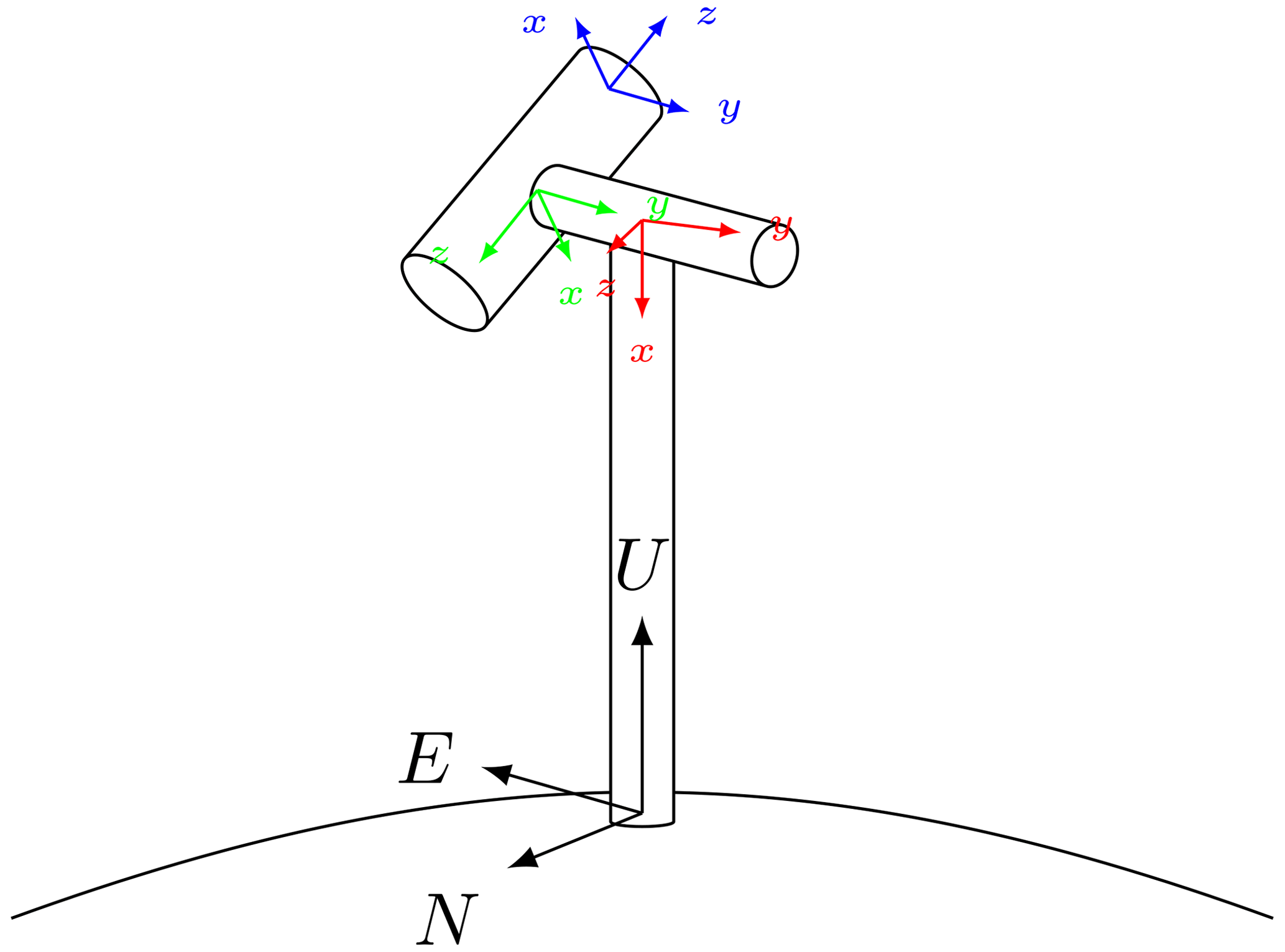
Figure 9Sketch of the SSARA instrument and the coordinate systems used for the mount calibration; ENU (black), MNT (red), GMB (green), and SH (blue).
In an ENU spherical coordinate system, the azimuth ϕ is zero in the north and increases towards the east, as one would expect. The polar angle is zero in the nadir and increases towards the zenith. Rotations between the coordinate systems are described by quaternions, where BqA is a quaternion-rotating coordinate system A to B.
For direct measurements with the quadrant sensor uniformly illuminated, the Sun and viewing vector in the ENU system are assumed to be equal (to within the accuracy of the Sun tracker). The Sun position in the ENU system is determined with the pyEphem Python package (Rhodes, 2011). It can calculate planetary positions to a precision satisfactory for our purpose using the VSOP87 model (Bretagnon and Francou, 1988). To obtain the viewing vector rv of the instrument, the unit vector in z direction (ez) in the SH system has to be transformed as follows:
The optimal rotation quaternion can be found by minimizing the distance between viewing vectors rv and Sun vector rs:
However, ENUqSH is composed of several rotations:
GMBqSH is defined as a 180∘ rotation around the local y axis to obtain the sensor head coordinate system. The active component of the mount acts on MNTqGMB. It contains the rotation angles of the azimuth and elevation motors (Δϕ and Δϑ), as well as the zero-point offset angles of the motors (ϑ0 and ϕ0). ϕ0 is zero due to our definition of the MNT system (it is effectively absorbed into ENUqMNT), but ϑ0 has to be determined. Both offset angles are constant over time and do not change for instrument realignment. Furthermore, the non-perpendicularity δ between the two motors is considered.
ENUqMNT is unknown and contains the tilt and rotation of the mount. It changes every time the instrument is moved, involving a new calibration. The minimization now has six variables (four components of ENUqMNT, δ, and ϑ0), and one constraint (ENUqMNT has to be normed). This can be achieved using the sequential least squares programming (SLSQP) algorithm (Kraft, 1988).
For the A-LIFE data, the fitting determines a non-perpendicularity of the motors δ of 0.95∘ and an elevation offset ϑ0 of −6.46∘. The rotation quaternion ENUqMNT is reconstructed to (0.704, −0.044, −0.707, 0.043). While the non-perpendicularity and the elevation offset are constant over time, the rotation quaternion will change every time the instrument is moved.
Figure 10 shows the remaining deviation between the fitted instrument pointing and the actual Sun position for all measurements in the A-LIFE campaign. The calibration is accurate to within 32 arcmin. The remaining inaccuracies are most likely due to the limited precision of the quadrant sensor and the way the instrument is tracking the Sun. The sensor has to pick up on brightness differences across the solar disk. Also, high aerosol loads, cirrus, or thin water clouds blur out the solar disk, resulting in an uniformly illuminated four-quadrant sensor further away from the Sun's center. If the clouds are “streaky”, this effect can occur in a certain direction. To avoid oscillation of the sensor head, the correction of pointing is damped. As a result, the instrument will most likely point to the lower left of the solar disk in the morning and the upper left in the evening. Other disruptions might occur by the instrument having to “search” the Sun after every scan. In the future, this effect should be minimized by using online fitting of the mount skewness. Furthermore, the change of the apparent solar position due to atmospheric refraction has been ignored.

Figure 10Residual between calibrated and calculated Sun positions. The average apparent size of Sun disk is used as reference (grey).
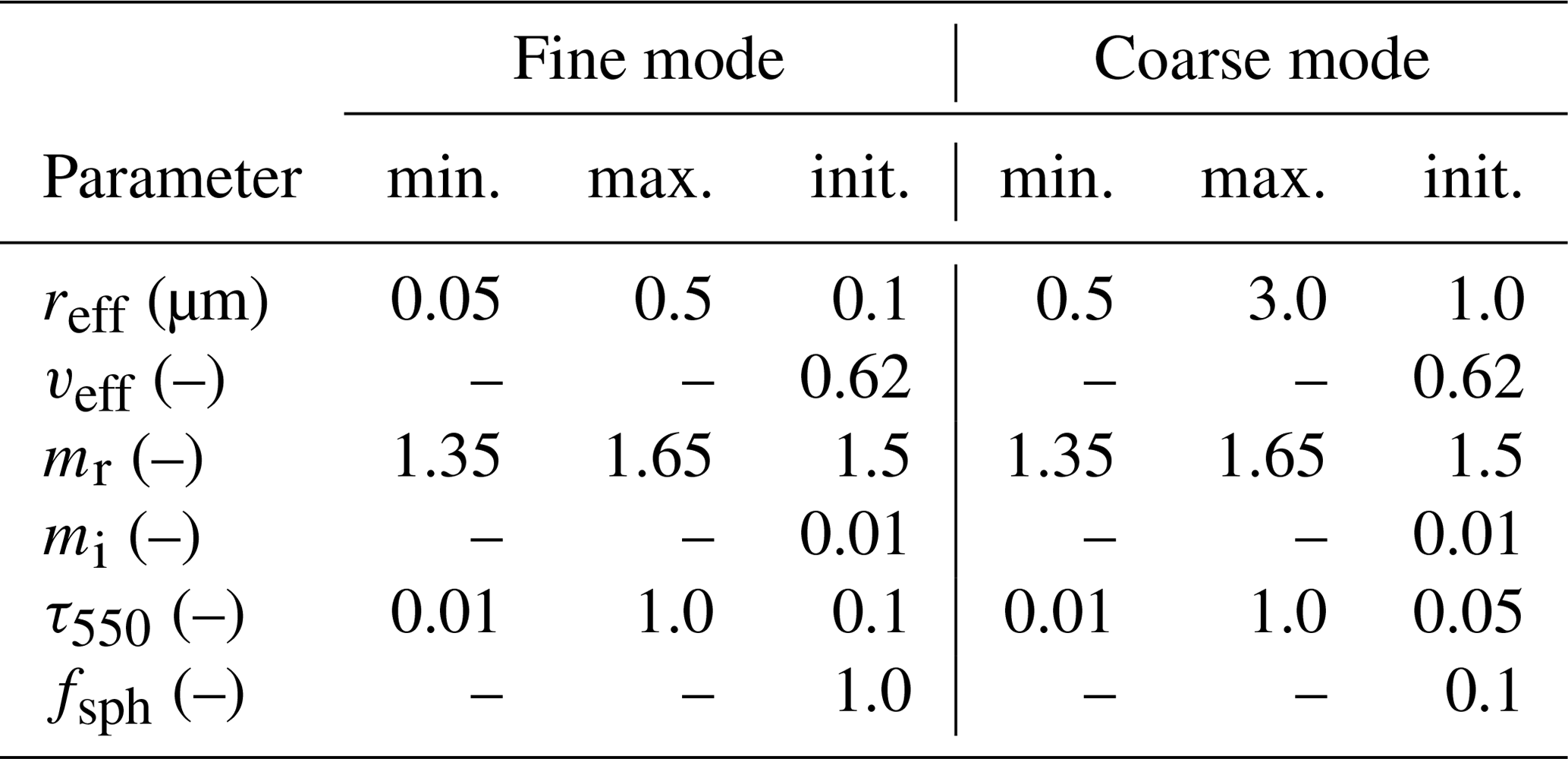
Table 3Boundaries and initial values for the aerosol parameters used in the retrieval. For effective variance (veff), the imaginary part of the refractive index (mi), and the fraction of spherical particles (fsph), no bounds are given, as these quantities are fixed.
2.2.3 Langley calibration
Langley extrapolation is a method to enable Sun photometers to retrieve the total optical depth of the atmosphere, without the need for a radiometric calibration of the instrument in a laboratory (Forgan, 1994). The basis for the extrapolation is the Bouguer–Lambert–Beer law and its logarithmic representation:
where I and I0 are the measured and extraterrestrial irradiance, respectively. τ is the optical depth, and m the air mass factor. The latter describes the increase in the direct optical pathlength – and therefore the optical depth – from the Sun to the detector. In the simplest geometric approach, , with the solar zenith angle Θ. A more elaborate air mass model taking into account atmospheric refraction and the curvature of the Earth can be found in Kasten and Young (1989). Additionally, the extraterrestrial irradiance I0 has to be corrected for the seasonal variability in Sun–Earth distance (Spencer, 1971).

Figure 11HaloCam images for 17 April 2017. The convective clouds in the early morning and afternoon are visible. The persisting cirrus clouds towards the evening can be seen.
Taking measurements at varying values of the air mass factor, and assuming the optical depth to be constant over time, the logarithm of the irradiance in Eq. (28) can be fitted as a linear function of m with slope τ. Extrapolating the linear fit to m=0 yields ln (I0). This value can then be used for reconstructing τ from measurements of I. Since only the ratio of the irradiances I and I0 is used, they can be replaced by any detector signal S that is linear in I.
with and .
This τ is the combined value of Rayleigh (τR), trace gas (τM), aerosol (τA), and possibly cloud (τC) optical depths. The contribution from Rayleigh was determined according to Bodhaine et al. (1999), scaled with the measured air pressure. At around 500 nm, O3 and NO2 are the main contributors to the trace gas optical depth τM. Their profiles were taken from Anderson et al. (1986) and the corresponding absorption cross-sections from Bogumil et al. (2003). Assuming that no clouds are present, subtracting these components from the total optical depth leaves only the contribution from aerosol.
SSARA is usually calibrated once a year, either around March/April or around October/November at UFS Schneefernerhaus (2650 m) on Zugspitze. Firstly, at this height, the contamination by boundary layer aerosols is minimal. Also, early/late in the year, convective processes over the measurement site are not prominent. Therefore, temporal homogeneity of τ is found more frequently during that time. The calibration used for the data presented in this paper was done in November 2016.
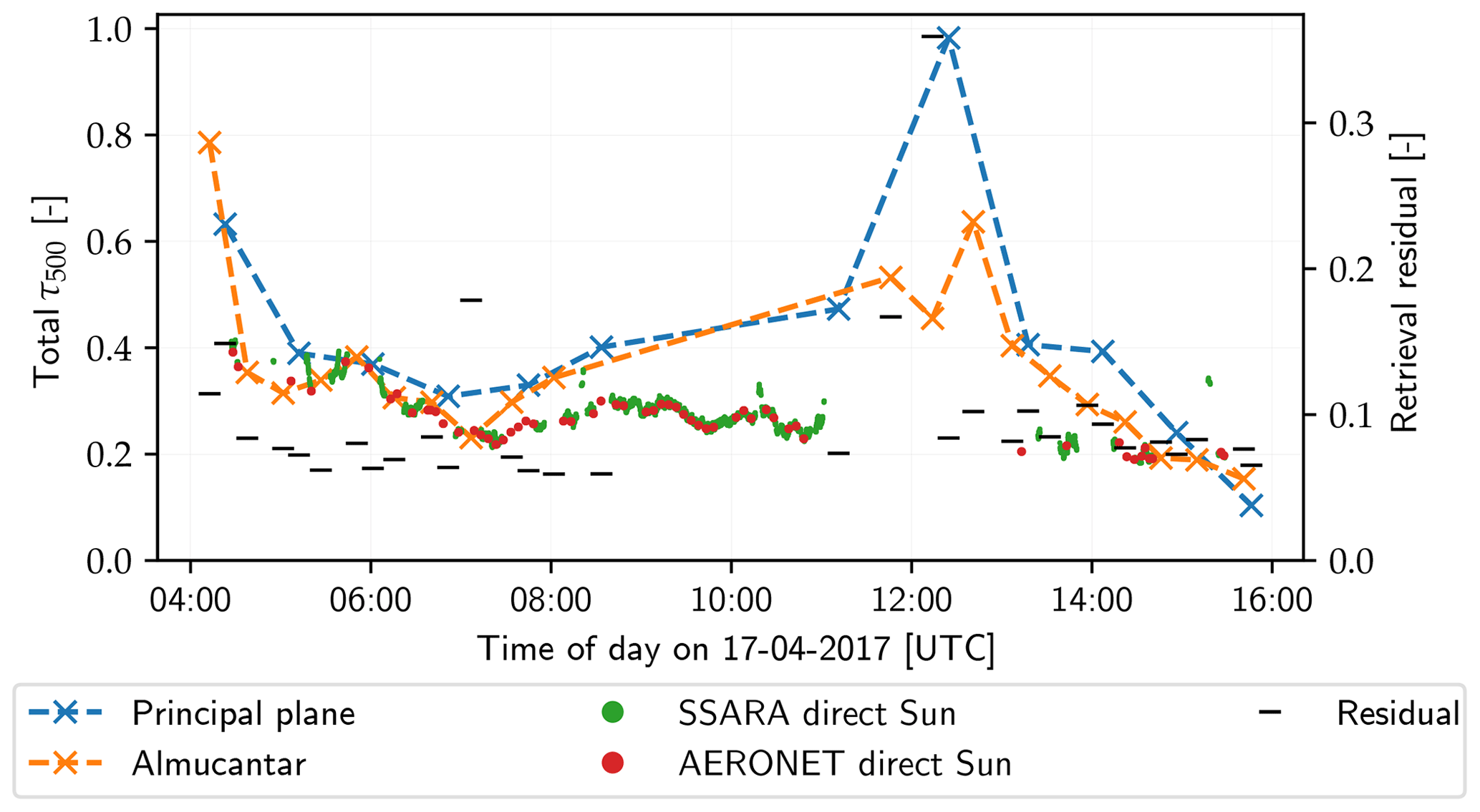
Figure 12Total AOD at 500 nm for 17 April 2017. Crosses indicate values retrieved from SSARA almucantar (orange) and principal plane (blue) scans. Green and red dots are from direct Sun observations with SSARA and AERONET, respectively. Note the agreement of these observations between the two instruments. The thin black markers represent the residual of the retrieved solution.
3.1 Retrieval algorithm
Our algorithm (Grob et al., 2019) minimizes the difference between observed polarized sky radiances and corresponding forward model simulations by varying aerosol properties. These retrieved aerosol parameters are effective radius reff, real part of the refractive index mr, and AOD at 550 nm τ550 for two aerosol modes with a log-normal particle size distribution. Each of these quantities is retrieved separately for both modes. Table 3 shows all the initial values and retrieval limits for all parameters of the aerosol model. If no boundaries are given, the parameter is not varied but fixed to its initial value. These are the effective variance of the particle size distribution veff, the imaginary part of the refractive index mi, and the fraction of spherical particles fsph. The retrieval has previously been validated with synthetic observations of a variety of clear-sky and cloudy situations with varying aerosols (Grob et al., 2019).

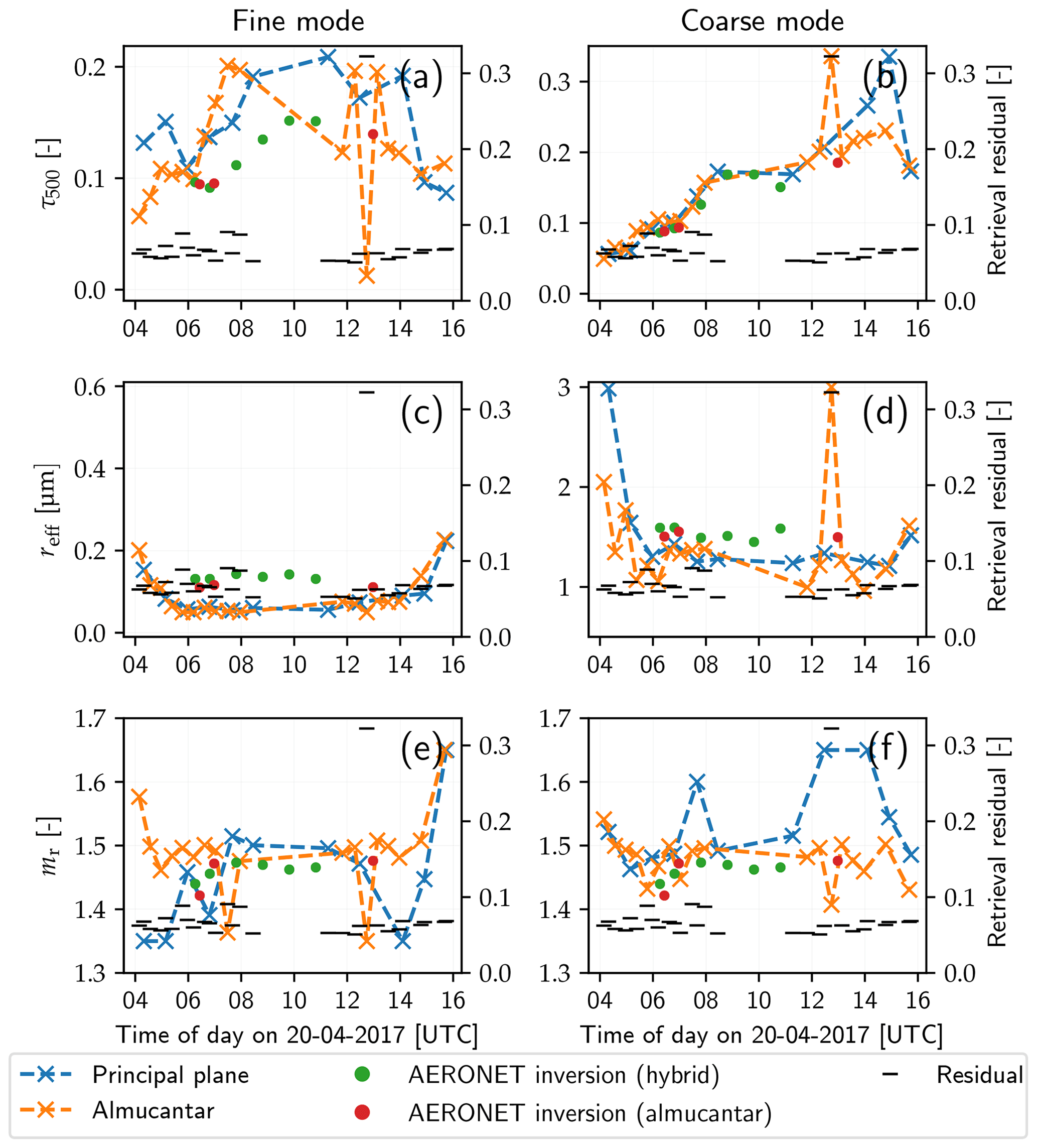
Figure 13Fine- and coarse-mode trends of aerosol optical depth (τ500), mode effective radius (reff), and real part of refractive index (mr) for 17 April 2017. Values obtained from principal plane scans are marked by blue crosses; those from almucantar scans are orange. The residual of the retrieval is shown by black markers. AERONET version 3 level 1.5 inversion results are shown as green and red dots, corresponding to retrieval of almucantar and hybrid scans, respectively. The refractive index is assumed to be equal for both modes in the AERONET retrieval.
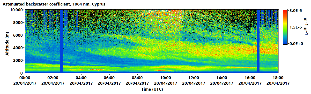
Figure 14The 1064 nm attenuated backscatter (in ) measured by a PollyXT lidar at the LACROS site on 20 April 2017.
However, for this study, several changes have been made compared to Grob et al. (2019) to better adapt the retrieval algorithm to measurements. Firstly, we assume a mixture of spherical and non-spherical particles for the coarse mode. This is more realistic for many aerosols (e.g., Dubovik et al., 2006, and references therein). The optical properties of this mixture are calculated by linear mixing of the tabulated optical properties for spheres and spheroids from Dubovik et al. (2006). They describe spheroids as a mixture of particles with aspect ratios ranging from 0.3 (elongated) to 3.0 (flattened). The fine mode is still assumed to contain only spherical particles. A surface albedo of 0.15 at 550 nm was estimated from MODIS observations and is for simplicity used for all wavelengths.
Additionally, the cloud screening has been revised. Due to the higher level of noise in the measurements, the original method classified too many measurements as cloudy. Furthermore, SSARA also provides unpolarized radiance measurements at 440 and 780 nm usable for cloud detection. In the new version, a set of 500 simulations of the given scan geometry is performed with aerosol parameters randomly sampled from the ranges given in Table 3. For simplicity and computational speed, only a single aerosol mode is used in these forward simulations. For every wavelength, the measured total radiance and its derivative with respect to the scattering angle are compared to these simulations. If the measured quantities are not within the 95th percentile of the simulated values, the measurement at this angle is flagged as cloudy. The same is done for the DoLP at 500 nm. This gives four separate cloud masks, three from unpolarized radiances at 440, 500 and 780 nm, and one from the DoLP at 500 nm. If more than two of them indicate a cloud at a certain scan angle, this data point is removed from the scan for the subsequent retrieval. This multi-stage approach makes the method robust against noise but still strict enough to reliably remove observations of clouds.
Finally, the measurement scans performed with SSARA during the A-LIFE campaign are not taken at equidistant scattering angles. Similar to scans performed by instruments in the AERONET framework, the angular sampling rate is higher around the Sun. This results in this area being overrepresented and therefore overweighted in the minimization procedure. However, most of the information provided by polarization is contained in measurements at larger scattering angles. To account for this, all measurements are weighted by the inverse of their angular sampling rate:
where wi is the weight of the ith measurement point, and ϑi the corresponding scattering angle.
3.2 Case studies
The following measurements have been performed during the A-LIFE field campaign. SSARA was installed on top of a building of the University of Cyprus in Limassol (34.674∘ N, 33.040∘ E). The AERONET station CUT-TEPAK is installed about 300 m to the east. The Leipzig Aerosol and Cloud Remote Observations System (LACROS; Bühl et al., 2013), including a PollyXT lidar system (Engelmann et al., 2016), was located 400 m to the northeast.
Between 6 and 28 April, SSARA continuously performed direct Sun observations. These have been interleaved with sky radiance scans in the almucantar and principal plane at pre-selected solar zenith angles. Almucantar plane scans have been carried out at every 5∘ of solar zenith angle between 35 and 80∘, and in the principal plane at 10∘ intervals between 30 and 80∘. The data of channel 11 (1020 nm) were excluded from the analysis as they intermittently provided faulty values during the measurement campaign.
For testing our retrieval, data from 17 and 20 April were selected for more in depth case studies. To evaluate the retrieval performance, the same criteria were used as in the numerical studies. These were taken from Mishchenko et al. (2004) and allow for a maximum deviation of 0.04 or 10 % deviation in AOD, 0.1 µm or 10 % in effective radius, and 0.02 in the refractive index. Since the true value is unknown, the results were compared with the AOD retrieved from direct Sun observations and the level 1.5 data of the AERONET version 3 inversion. Level 1.5 data were used, since level 2.0 did not include refractive index values for the chosen dates. It should be noted that the AERONET inversion uses the same refractive index for both modes.
Since the plots showing the results are the same for both days, they will be described here first. Figures 12 and 15 show the aerosol optical depth at 500 nm for these 2 d. Orange and blue crosses mark values retrieved by the inversion from principal plane and almucantar scans, respectively. Since the total error of the retrieved values cannot easily be estimated, we show the residual of the minimization as an indicator of the performance of the retrieval for a given measurement. The values obtained from direct Sun observations are displayed as reference, with green dots representing AERONET L2 data and the red ones SSARA measurements. For both days, these measurements agree well between the two instruments. Figures 13 and 16 show all retrieved aerosol parameters for fine and coarse modes, separately. Again, blue corresponds to values obtained from principal plane and orange to those from almucantar scans. The black tick marks show the residual of the fit. The AERONET points are the results of the AERONET inversion for hybrid (red; see Giles et al., 2019) and almucantar scans (green). Since AERONET uses a common refractive index for fine and coarse modes, this value is shown for both modes (subplots e and f). It should amount to a weighted mean of the values we retrieved for the two modes and therefore lie somewhere between those. To facilitate the comparison of the retrieval results with direct Sun measurements and AERONET values, the optical depth is evaluated at 500 nm in the following case studies.
3.2.1 Cloudy day (17 April 2017)
17 April was chosen to illustrate the retrieval behavior during cloudy phases. Around sunrise and between roughly 11:00 and 14:15 UTC, convective clouds have been present at the measurement site. This can also be deduced from the gap in AERONET direct Sun AOD data shown in Fig. 12. Cirrus clouds already appeared around 10:30 UTC and persisted almost until 16:00 UTC. Figure 11 shows four snapshots of the cloud situation during that day. The pictures have been taken with the sky camera HaloCam (Forster et al., 2017) installed coaxially with the SSARA sensor head.
In the early morning (until around 04:30 UTC; Fig. 12), an increased AOD is retrieved. This coincides with the presence of convective clouds also visible in the top left panel of Fig. 11. As shown in sensitivity studies (Grob et al., 2019), these might lead to an overestimation of the AOD. However, it could indicate that additionally the AOD is increased, for example, due to hygroscopic growth of aerosol particles in humid air. The same can be observed in Fig. 12 for the convective period in the afternoon between 11:00 and 13:00 UTC. Here, it should be noted that for the corresponding scans, the residual is sometimes slightly higher, indicating a less reliable retrieval result. This is shown by the black tick marks in Figs. 12 and 13. Most of the time, the residual is below 0.1 but spikes up to 0.4. Until around 07:00 UTC, the retrieved total AOD is consistent with the values obtained from direct Sun measurements. Starting around this time, the AOD is overestimated by up to 0.1 during clear-sky periods. Small gaps in the AERONET direct measurements indicate the presence of clouds or high variability in the aerosol. Again, some deviation in the retrieval (generally overestimation) is to be expected here. Towards the evening, the optical depth seems to be underestimated. Note that perfect agreement between the values retrieved from sky radiance observation and from direct Sun observations cannot be expected. The reason for this might be spatial inhomogeneity of the aerosol properties (maritime towards ocean, anthropogenic aerosols towards city/industry). Other explanations could be measurement errors or systematic effects of the retrieval. This can also explain the differences between the results of almucantar and principal plane scans.
In Fig. 13a and b, the AOD is separated into fine and coarse modes. Over the entire day, the aerosol optical depth is dominated by the fine mode. This compares well to the AERONET inversion data points. The contribution of the coarse mode is larger compared to AERONET. It should be noted here that – in contrast to the AERONET inversion – we do not use the total AOD from direct Sun observations as a constraint for our minimization because the method is designed to be employed in cloudy situations, where such measurements are not available.
The retrieved effective radius of the fine mode (Fig. 13c) is mostly consistent over the entire day, including the cloudy period in the afternoon. This insensitivity of the effective radius to the presence of clouds was also observed in the numerical studies (Grob et al., 2019). However, the increased values in the morning and evening should be noted. This seems to be a systematic pattern; the reason for this is still unknown. When compared to AERONET, our fine-mode effective radii are somewhat smaller but within the 0.1 µm limit. An underestimation is also observed for the coarse mode (Fig. 13d). Here, the AERONET inversion suggests the presence of large particles with an effective radius of around 2 µm between 07:00 and 10:00 UTC. The values we obtain are smaller. Although previous sensitivity studies have shown that our retrieval has the tendency to underestimate the size of large coarse-mode particles, independent measurements would be needed to further investigate the discrepancy.
The retrieved real part of the refractive index changes rapidly for fine-mode particles (Fig. 13e). High values can be observed in the aforementioned times with clouds present. This behavior is again consistent with the results of the numerical studies, where clouds induce an overestimation of the index of refraction. The results for the coarse mode (Fig. 13f) are smoother in general. The retrieved value mostly stays close to the prior of 1.5, which might be caused by a low sensitivity to this parameter. The refractive index derived from AERONET ranges from 1.33 to 1.48. At around 07:00 UTC, there is an obvious discrepancy between values obtained from hybrid and almucantar scans. The values below 1.35 between 08:30 and 10:00 UTC seem unrealistic, as all expected aerosol types have a higher refractive index.
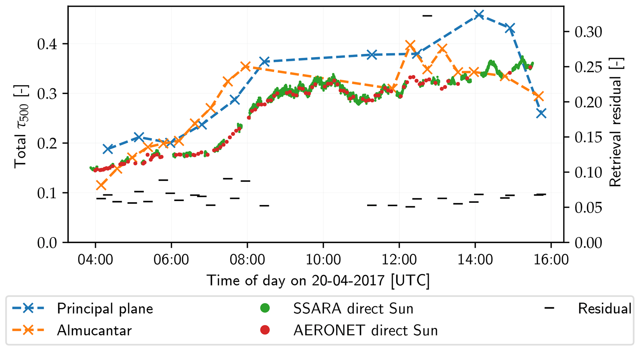
3.2.2 Clear-sky day with arriving Saharan dust layer (20 April 2017)
20 April was a clear-sky day. Starting in the late morning (07:00 UTC, 10:00 LT), the AOD increased. This can be attributed to the arrival of a Saharan dust outbreak over Cyprus from the west. Figure 14 shows the attenuated backscatter at 1064 nm of the PollyXT lidar. An aerosol layer is visible between roughly 2 and 5 km, beginning with thin filaments at around 04:00 UTC, and increasing in thickness towards noon. PollyXT also provides measurements of the particle linear depolarization ratio (PLDR) at 532 nm that can be used to discriminate between types of aerosol (Baars et al., 2016). In this layer, PLDR values around 25 % are observed and clearly identify the aerosol as desert dust (Müller et al., 2003; Freudenthaler et al., 2009).
With the exception of the early morning and evening, the AOD derived from the inversion of SSARA sky radiance measurements is overestimated by sometimes more than 0.1, when compared with the values obtained from direct Sun observations from SSARA and AERONET (see Fig. 15). Additionally, the results from almucantar and principal plane differ significantly, with neither of them preferable to the other. Judging from the residual, the results are all equally trustworthy, barring one exception at approximately 13:00 UTC.
An increase in the coarse-mode AOD is clearly visible in Fig. 16b, starting at around 07:00 UTC. The retrieved values agree well with the AERONET inversion results. This increase is consistent with the arrival of Saharan dust which contains larger particles. Consequently, the overestimation of the total AOD retrieved from SSARA sky radiance measurements has to be caused by the fine mode (see Fig. 16a). Also it is not consistently retrieved from principal plane and almucantar scan patterns. Again, the deviation in the retrieved total AOD from the direct Sun observations is due to the fact that this value is not used as a constraint in the inversion.
The effective radius of the fine mode (see Fig. 16c) is stable over most of the day, only increasing in the morning and the evening again. AERONET finds larger fine-mode particles, again by up to about 0.1 µm. Apart from the single outlier at 13:00 UTC, coarse-mode effective radius is retrieved quite consistently over the entire day (Fig. 16d). Also, it agrees well with the AERONET inversion results. For values around 1.5 µm, the retrieval proved to be reliable in the sensitivity studies. Here, an increase in morning and evening is visible as well.
For the real part of the refractive index (Fig. 16e and f), most measurements indicate a value of around 1.5 for both fine and coarse modes. This agrees well with the AERONET inversion, which produces only slightly lower values. However, since this is also the prior and large discrepancies between values derived from the two scan patterns are visible, this might also be the result of lacking sensitivity to this parameter.
The retrieval of microphysical and optical properties of aerosols from multispectral sky radiance observations remains a challenge, especially in cloudy conditions. Recently, the use of polarimetric information has proven to provide additional information. We introduce a new inversion method using such measurements. However, polarimetric measurements pose additional demands on the instruments, their setup and calibration. In this paper, we also present new methods to lower the effort of calibrating such an instrument and its mount. These methods are applicable to other instruments as well.
We introduced a new method for polarimetric calibration of polarized Sun and sky radiometers. In contrast to previous calibration methods, it can simultaneously determine orientation and diattenuation of a polarized channel. This reduces the experimental effort, as only measurements at a single degree of polarization are necessary. Additionally, neither correction factors nor assumptions about the filters are required. For the calibration of our Sun photometer SSARA, the diattenuation of the linear polarizers was determined to an accuracy of 0.002 and their rotation to within 0.1∘. Neglecting these filter parameters would introduce a systematic relative error of up to ±1 % in total radiance and ±2 % in DoLP across the hemisphere.
A novel quaternion-based correction of the mount skewness reduces the pointing error of the instrument to below 32 arcmin. This is limited by the accuracy of SSARA's Sun tracker and could be improved with a more sophisticated one. The correction can be applied in post-processing, reducing the demands on the accuracy of the setup of the mount. Alternatively, it can be used in real time during the operation of the instrument, allowing for more precise pointing during cloudy days.
For evaluating our retrieval using polarimetric information, 2 d of SSARA measurements from the A-LIFE field campaign have been selected for more in-depth analysis. The SSARA instrument has been calibrated with the aforementioned methods. The retrieval has been applied on principal plane and almucantar scans separately. On both days, the results differ depending on the scan pattern used, the reason for which is not fully understood.
The first case study investigates the retrieval's behavior under partly cloudy conditions. An increase in AOD is visible around the time of convective activity. This effect has been shown to exist due to 3-D radiative effects close to clouds in previous numerical studies. The second day selected features clear-sky conditions with an appearing Saharan dust layer. This layer can be observed by an increase in coarse-mode AOD retrieved from SSARA measurements, as well as in AERONET inversion data. With a few exceptions, the retrieval shows the tendency to overestimate the AOD when compared to values obtained from direct Sun observations. The error sometimes exceeds 0.1 in total AOD. The retrieval of the effective radius works well for the fine mode. In both cases, the value is slightly too low but agrees with AERONET to within 0.1 µm. In the coarse mode, the inversion compares well to AERONET for values around 1.5 µm. For larger particles (towards effective radii of 2 µm), our retrieval produces smaller radii than AERONET. There appears to be a systematic increase in the retrieved effective radius for both modes in the morning and evening. To properly evaluate these results and resolve the remaining discrepancies, independent measurements are required. The same is true for the retrieval of index of refraction, especially due to the fact that AERONET uses a common value for both modes. In some cases, our results are well supported by AERONET. However, the index of refraction often stays close to its prior, which could indicate lacking sensitivity to that parameter that was also found in the sensitivity study by Grob et al. (2019).
These remaining differences in the retrieved parameters between our method and the AERONET inversion have to be examined further. As a first step, the results from A-LIFE should be compared to measurements obtained from independent instruments, such as lidar or in situ. This should also extend to times where no AERONET results are available for comparison. Moreover, our inversion scheme should be applied to measurements from other sky radiometers, such as the Cimel CE318-DP used in AERONET. This is to rule out instrument effects. However, due to the high level of precision achieved in the various calibration steps, this is an unlikely source of error. Also, the retrieval could then be evaluated using multiple polarized wavelength measurements. Vice versa, our measurements might be analyzed using different inversion algorithms. This way, systematic errors in the retrieval method can be identified. Further numerical studies with respect to the influence of the scan pattern on the retrieval results are recommended. Additionally, it would be possible to add the total AOD obtained from direct Sun observations as a constraint to our retrieval. This approach might limit the applicability to cloudy situations when no such measurements are available or the value changes rapidly. However, for clear-sky cases, this constraint would certainly improve the retrieval results. Nonetheless, our polarimetric calibration method could easily be adapted to instruments used in AERONET.
Quaternions are an extension to complex numbers. As complex numbers can be used to describe operations – such as rotation – in 2-D space (in polar notation), the same is true for quaternions in 3-D space (see Horn, 1987). A quaternion is described by four real components:
where i, j, and k are the imaginary units with the following identities:
Quaternions form a non-abelian group under multiplication defined by the Hamilton product. Therefore, quaternions do not commute under the Hamilton product. It can be derived using the distributive and associative laws, and the identities in Eq. (A2).
Additionally, a dot product is defined as
It can be used to induce a norm, . A quaternion is conjugated by inverting the sign of its imaginary components:
It can be shown that the multiplicative inverse is
As a result, for normed quaternions (∥q∥=1), its inverse is its conjugate.
Quaternions describing spatial rotations in three-dimensional space have to be normed. A rotation about an axis a through an angle α is represented by the quaternion:
It can easily be seen that the conjugate is in fact the inverse, corresponding to a rotation by the negative angle or around the negative axis. According to Euler's rotation theorem, the conjunction of several rotations can be described by a single rotation. This also follows from the group properties of quaternions. The Hamilton product of two normed quaternions is again a normed quaternion, representing a rotation.
A regular 3-D Euclidian vector r can be described by a quaternion with q0 = 0 and q1, q2, and q3 being the Euclidian vector components in x, y, and z directions (“pure” quaternion). The rotation by a quaternion is calculated as
The resulting quaternion is again pure, and the rotated vector can be reconstructed. Also, unit quaternions can be transformed into a rotation matrix that can be applied to regular Euclidean vectors. For a unit quaternion q, the Euler angles of the corresponding rotation and the 3×3 rotation matrix Mq are given by
All SSARA measurement data taken during the A-LIFE field campaign in Cyprus during April 2017 are available at https://doi.org/10.5281/zenodo.3607218 (Grob, 2020). The dataset includes the raw instrument data (L0), the calibrated measurements (L1), and retrieved aerosol optical thickness (AOT) from direct Sun measurements.
HG developed the code for the retrieval and the calibration, performed the calibration, processed the measurement data, and prepared the manuscript. MW and MS designed and built the SSARA instrument, respectively. LF contributed to the polarization equipment of the instrument. CE and BM assisted the interpretation of the results. CE, MW, MS, and BM also contributed to the manuscript. CE and BM prepared the proposal for the DFG project.
The authors declare that they have no conflict of interest.
The work for this paper was funded through the German Research Foundation (DFG) project 264269520 “Neue Sichtweisen auf die Aerosol-Wolken-Strahlungs-Wechselwirkung mittels polarimetrischer und hyper-spektraler Messungen”. We thank Tobias Kölling and Markus Garhammer for their help with the calibration of the instrument. Carlos Toledano and his team operated and maintained SSARA during most of the A-LIFE campaign. The authors thank Holger Baars, Birgit Heese, and the PollyXT team from the Leibniz Institute for Tropospheric Research (TROPOS) in Leipzig, Germany, for performing the lidar measurements in Cyprus, creating the corresponding plot, and helping with its interpretation. TROPOS acknowledges support from ACTRIS-2 under grant agreement no. 654109 from the European Union’s Horizon 2020 research and innovation program. The access to the LOA calibration facility, organized by Carlos Toledano, was possible thanks to the ACTRIS project. An application of Transnational Access was approved by the AERONET-Europe panel within ACTRIS. The authors also give thanks to Maxime Catalfamo and Luc Blarel for their support at LOA. We thank Diofantos Hadjimitsis and his staff for their effort in establishing and maintaining the CUT-TEPAK AERONET site.
This research has been supported by the Deutsche Forschungsgemeinschaft (grant no. 264269520).
This paper was edited by Udo Friess and reviewed by Gerard van Harten and one anonymous referee.
Albrecht, B. A.: Aerosols, Cloud Microphysics, and Fractional Cloudiness, Science, 245, 1227–1230, https://doi.org/10.1126/science.245.4923.1227, 1989. a
Anderson, G. P., Clough, S. A., Kneizys, F., Chetwynd, J. H., and Shettle, E. P.: AFGL atmospheric constituent profiles (0-120 km), Tech. rep., Air Force Geophysics Lab Hanscom AFB, MA, 1986. a
Baars, H., Kanitz, T., Engelmann, R., Althausen, D., Heese, B., Komppula, M., Preißler, J., Tesche, M., Ansmann, A., Wandinger, U., Lim, J.-H., Ahn, J. Y., Stachlewska, I. S., Amiridis, V., Marinou, E., Seifert, P., Hofer, J., Skupin, A., Schneider, F., Bohlmann, S., Foth, A., Bley, S., Pfüller, A., Giannakaki, E., Lihavainen, H., Viisanen, Y., Hooda, R. K., Pereira, S. N., Bortoli, D., Wagner, F., Mattis, I., Janicka, L., Markowicz, K. M., Achtert, P., Artaxo, P., Pauliquevis, T., Souza, R. A. F., Sharma, V. P., van Zyl, P. G., Beukes, J. P., Sun, J., Rohwer, E. G., Deng, R., Mamouri, R.-E., and Zamorano, F.: An overview of the first decade of PollyNET: an emerging network of automated Raman-polarization lidars for continuous aerosol profiling, Atmos. Chem. Phys., 16, 5111–5137, https://doi.org/10.5194/acp-16-5111-2016, 2016. a
Balois, J. Y.: Polarizing box POLBOX User’s Guide, Tech. rep., Laboratoire d'Optique Atmospherique, Lille, 1998. a
Bass, M., DeCusatis, C., Enoch, J., Lakshminarayanan, V., Li, G., Macdonald, C., Mahajan, V., and Van Stryland, E.: Handbook of Optics, Third Edition Volume II: Design, Fabrication and Testing, Sources and Detectors, Radiometry and Photometry, McGraw-Hill, Inc., New York, NY, USA, 3 edn., 2010. a
Bodhaine, B. A., Wood, N. B., Dutton, E. G., and Slusser, J. R.: On Rayleigh Optical Depth Calculations, J. Atmos. Ocean. Tech., 16, 1854–1861, https://doi.org/10.1175/1520-0426(1999)016<1854:ORODC>2.0.CO;2, 1999. a
Bogumil, K., Orphal, J., Homann, T., Voigt, S., Spietz, P., Fleischmann, O., Vogel, A., Hartmann, M., Kromminga, H., Bovensmann, H., Frerick, J., and Burrows, J.: Measurements of molecular absorption spectra with the SCIAMACHY pre-flight model: instrument characterization and reference data for atmospheric remote-sensing in the 230–2380 nm region, J. Photoch. Photobio. A, 157, 167–184, https://doi.org/10.1016/S1010-6030(03)00062-5, 2003. a
Bretagnon, P. and Francou, G.: Planetary theories in rectangular and spherical variables – VSOP 87 solutions, Astron. Astrophys., 202, 309–315, 1988. a
Bühl, J., Seifert, P., Wandinger, U., Baars, H., Kanitz, T., Schmidt, J., Myagkov, A., Engelmann, R., Skupin, A., Heese, B., Klepel, A., Althausen, D., and Ansmann, A.: LACROS: the Leipzig Aerosol and Cloud Remote Observations System, Proc. SPIE, 8890, https://doi.org/10.1117/12.2030911, 2013. a
Chandrasekhar, S.: Radiative Transfer, Dover books on physics and engineering, Dover Publications, Inc., 1950. a
de Haan, J. F., Bosma, P., and Hovenier, J.: The adding method for multiple scattering calculations of polarized light, Astron. Astrophys., 183, 371–391, 1987. a
Deschamps, P., Breon, F., Leroy, M., Podaire, A., Bricaud, A., Buriez, J., and Seze, G.: The POLDER mission: instrument characteristics and scientific objectives, IEEE T. Geosci. Remote, 32, 598–615, https://doi.org/10.1109/36.297978, 1994. a
Di Noia, A., Hasekamp, O. P., van Harten, G., Rietjens, J. H. H., Smit, J. M., Snik, F., Henzing, J. S., de Boer, J., Keller, C. U., and Volten, H.: Use of neural networks in ground-based aerosol retrievals from multi-angle spectropolarimetric observations, Atmos. Meas. Tech., 8, 281–299, https://doi.org/10.5194/amt-8-281-2015, 2015. a
Diner, D. J., Xu, F., Martonchik, J. V., Rheingans, B. E., Geier, S., Jovanovic, V. M., Davis, A., Chipman, R. A., and McClain, S. C.: Exploration of a Polarized Surface Bidirectional Reflectance Model Using the Ground-Based Multiangle SpectroPolarimetric Imager, Atmosphere, 3, 591–619, https://doi.org/10.3390/atmos3040591, 2012. a
Dubovik, O., Sinyuk, A., Lapyonok, T., Holben, B. N., Mishchenko, M., Yang, P., Eck, T. F., Volten, H., Muñoz, O., Veihelmann, B., van der Zande, W. J., Leon, J.-F., Sorokin, M., and Slutsker, I.: Application of spheroid models to account for aerosol particle nonsphericity in remote sensing of desert dust, J. Geophys. Res.-Atmos., 111, D11208, https://doi.org/10.1029/2005JD006619, 2006. a, b, c
Emde, C., Buras, R., Mayer, B., and Blumthaler, M.: The impact of aerosols on polarized sky radiance: model development, validation, and applications, Atmos. Chem. Phys., 10, 383–396, https://doi.org/10.5194/acp-10-383-2010, 2010. a
Emde, C., Barlakas, V., Cornet, C., Evans, F., Korkin, S., Ota, Y., Labonnote, L. C., Lyapustin, A., Macke, A., Mayer, B., and Wendisch, M.: IPRT polarized radiative transfer model intercomparison project – Phase A, J. Quant. Spectrosc. Ra., 164, 8–36, https://doi.org/10.1016/j.jqsrt.2015.05.007, 2015. a
Emde, C., Buras-Schnell, R., Kylling, A., Mayer, B., Gasteiger, J., Hamann, U., Kylling, J., Richter, B., Pause, C., Dowling, T., and Bugliaro, L.: The libRadtran software package for radiative transfer calculations (version 2.0.1), Geosci. Model Dev., 9, 1647–1672, https://doi.org/10.5194/gmd-9-1647-2016, 2016. a
Emde, C., Barlakas, V., Cornet, C., Evans, F., Wang, Z., Labonotte, L. C., Macke, A., Mayer, B., and Wendisch, M.: IPRT polarized radiative transfer model intercomparison project – Three-dimensional test cases (phase B), J. Quant. Spectrosc. Ra., 209, 19–44, https://doi.org/10.1016/j.jqsrt.2018.01.024, 2018. a
Engelmann, R., Kanitz, T., Baars, H., Heese, B., Althausen, D., Skupin, A., Wandinger, U., Komppula, M., Stachlewska, I. S., Amiridis, V., Marinou, E., Mattis, I., Linné, H., and Ansmann, A.: The automated multiwavelength Raman polarization and water-vapor lidar PollyXT: the neXT generation, Atmos. Meas. Tech., 9, 1767–1784, https://doi.org/10.5194/amt-9-1767-2016, 2016. a
Fedarenka, A., Dubovik, O., Goloub, P., Li, Z., Lapyonok, T., Litvinov, P., Barel, L., Gonzalez, L., Podvin, T., and Crozel, D.: Utilization of AERONET polarimetric measurements for improving retrieval of aerosol microphysics: GSFC, Beijing and Dakar data analysis, J. Quant. Spectrosc. Ra., 179, 72–97, https://doi.org/10.1016/j.jqsrt.2016.03.021, 2016. a
Forgan, B. W.: General method for calibrating sun photometers, Appl. Optics, 33, 4841–4850, https://doi.org/10.1364/AO.33.004841, 1994. a
Forster, L., Seefeldner, M., Wiegner, M., and Mayer, B.: Ice crystal characterization in cirrus clouds: a sun-tracking camera system and automated detection algorithm for halo displays, Atmos. Meas. Tech., 10, 2499–2516, https://doi.org/10.5194/amt-10-2499-2017, 2017. a
Freudenthaler, V., Esselborn, M., Wiegner, M., Heese, B., Tesche, M., Ansmann, A., Müller, D., Althausen, D., Wirth, M., Fix, A., Ehret, G., Knippertz, P., Toledano, C., Gasteiger, J., Garhammer, M., and Seefeldner, M.: Depolarization ratio profiling at several wavelengths in pure Saharan dust during SAMUM 2006, Tellus B, 61, 165–179, https://doi.org/10.1111/j.1600-0889.2008.00396.x, 2009. a
Giles, D. M., Sinyuk, A., Sorokin, M. G., Schafer, J. S., Smirnov, A., Slutsker, I., Eck, T. F., Holben, B. N., Lewis, J. R., Campbell, J. R., Welton, E. J., Korkin, S. V., and Lyapustin, A. I.: Advancements in the Aerosol Robotic Network (AERONET) Version 3 database – automated near-real-time quality control algorithm with improved cloud screening for Sun photometer aerosol optical depth (AOD) measurements, Atmos. Meas. Tech., 12, 169–209, https://doi.org/10.5194/amt-12-169-2019, 2019. a, b
Grob, H.: SSARA A-LIFE measurement data (Version V1.0.0) [Data set], Zenodo, https://doi.org/10.5281/zenodo.3607219, 2020. a
Grob, H., Emde, C., and Mayer, B.: Retrieval of aerosol properties from ground-based polarimetric sky-radiance measurements under cloudy conditions, J. Quant. Spectrosc. Ra., 228, 57–72, https://doi.org/10.1016/j.jqsrt.2019.02.025, 2019. a, b, c, d, e, f
Hasekamp, O. P. and Landgraf, J.: Retrieval of aerosol properties over land surfaces: capabilities of multiple-viewing-angle intensity and polarization measurements, Appl. Optics, 46, 3332–3344, https://doi.org/10.1364/AO.46.003332, 2007. a
Hasekamp, O. P., Litvinov, P., and Butz, A.: Aerosol properties over the ocean from PARASOL multiangle photopolarimetric measurements, J. Geophys. Res.-Atmos., 116, D14204, https://doi.org/10.1029/2010JD015469, 2011. a
Holben, B., Eck, T., Slutsker, I., Tanré, D., Buis, J., Setzer, A., Vermote, E., Reagan, J., Kaufman, Y., Nakajima, T., Lavenu, F., Jankowiak, I., and Smirnov, A.: AERONET – A Federated Instrument Network and Data Archive for Aerosol Characterization, Remote Sens. Environ., 66, 1–16, https://doi.org/10.1016/S0034-4257(98)00031-5, 1998. a
Horn, B. K. P.: Closed-form solution of absolute orientation using unit quaternions, J. Opt. Soc. Am. A, 4, 629–642, https://doi.org/10.1364/JOSAA.4.000629, 1987. a
IPCC: Climate Change 2013: The Physical Science Basis. Contribution of Working Group I to the Fifth Assessment Report of the Intergovernmental Panel on Climate Change, Cambridge University Press, Cambridge, United Kingdom and New York, NY, USA, https://doi.org/10.1017/CBO9781107415324, 2013. a
Kasten, F. and Young, A. T.: Revised optical air mass tables and approximation formula, Appl. Optics, 28, 4735–4738, https://doi.org/10.1364/AO.28.004735, 1989. a
Kraft, D.: A Software Package for Sequential Quadratic Programming, DFVLR-FB 88-28, DFVLR Insitut für Dynamik der Flugsysteme, 1988. a
Li, L., Li, Z., Li, K., Blarel, L., and Wendisch, M.: A method to calculate Stokes parameters and angle of polarization of skylight from polarized CIMEL sun/sky radiometers, J. Quant. Spectrosc. Ra., 149, 334–346, https://doi.org/10.1016/j.jqsrt.2014.09.003, 2014. a, b
Li, Z., Blarel, L., Podvin, T., Goloub, P., and Chen, L.: Calibration of the degree of linear polarization measurement of polarized radiometer using solar light, Appl. Optics, 49, 1249–1256, https://doi.org/10.1364/AO.49.001249, 2010. a, b
Li, Z., Li, K., Li, L., Xu, H., Xie, Y., Ma, Y., Li, D., Goloub, P., Yuan, Y., and Zheng, X.: Calibration of the degree of linear polarization measurements of the polarized Sun-sky radiometer based on the POLBOX system, Appl. Optics, 57, 1011–1018, https://doi.org/10.1364/AO.57.001011, 2018. a, b, c
Mayer, B.: Radiative transfer in the cloudy atmosphere, Eur. Physical J. Conf., 1, 75–99, https://doi.org/10.1140/epjconf/e2009-00912-1, 2009. a
Mayer, B. and Kylling, A.: Technical note: The libRadtran software package for radiative transfer calculations – description and examples of use, Atmos. Chem. Phys., 5, 1855–1877, https://doi.org/10.5194/acp-5-1855-2005, 2005. a
Mishchenko, M. I., Cairns, B., Hansen, J. E., Travis, L. D., Burg, R., Kaufman, Y. J., Martins, J. V., and Shettle, E. P.: Monitoring of aerosol forcing of climate from space: analysis of measurement requirements, J. Quant. Spectrosc. Ra., 88, 149–161, https://doi.org/10.1016/j.jqsrt.2004.03.030, 2004. a
Müller, D., Mattis, I., Wandinger, U., Ansmann, A., Althausen, D., Dubovik, O., Eckhardt, S., and Stohl, A.: Saharan dust over a central European EARLINET-AERONET site: Combined observations with Raman lidar and Sun photometer, J. Geophys. Res.-Atmos., 108, 4345, https://doi.org/10.1029/2002JD002918, 2003. a
Rhodes, B. C.: PyEphem: astronomical ephemeris for Python, Astrophysics Source Code Library, 2011. a
Riesing, K. M., Yoon, H., and Cahoy, K. L.: Rapid telescope pointing calibration: a quaternion-based solution using low-cost hardware, Journal of Astronomical Telescopes, Instruments, and Systems, 4, 034002, https://doi.org/10.1117/1.JATIS.4.3.034002, 2018. a
Seefeldner, M., Oppenrieder, A., Rabus, D., Reuder, J., Schreier, M., Hoeppe, P., and Köpke, P.: A Two-Axis Tracking System with Datalogger, J. Atmos. Ocean. Tech., 21, 975–979, https://doi.org/10.1175/1520-0426(2004)021<0975:ATTSWD>2.0.CO;2, 2004. a
Spencer, J. W.: Fourier Series Representation of the Position of the Sun, Search, 2, 172, 1971. a
Toledano, C., Wiegner, M., Garhammer, M., Seefeldner, M., Gasteiger, J., Müller, D., and Köpke, P.: Spectral aerosol optical depth characterization of desert dust during SAMUM 2006, Tellus B, 61, 216–228, https://doi.org/10.1111/j.1600-0889.2008.00382.x, 2009. a
Toledano, C., Wiegner, M., Groß, S., Freudenthaler, V., Gasteiger, J., Müller, D., Müller, D., Schladitz, A., Weinzierl, B., Torres, B., and O’Neill, N. T.: Optical properties of aerosol mixtures derived from sun-sky radiometry during SAMUM-2, Tellus B, 63, 635–648, https://doi.org/10.1111/j.1600-0889.2011.00573.x, 2011. a
van Amerongen, A., Rietjens, J., Smit, M., van Loon, D., van Brug, H., van der Meulen, W., Esposito, M., and Hasekamp, O.: Spex the Dutch roadmap towards aerosol measurement from space, Proc. SPIE, 10562, https://doi.org/10.1117/12.2296227, 2017. a
van Harten, G., Snik, F., Rietjens, J. H. H., Smit, J. M., de Boer, J., Diamantopoulou, R., Hasekamp, O. P., Stam, D. M., Keller, C. U., Laan, E. C., Verlaan, A. L., Vliegenthart, W. A., ter Horst, R., Navarro, R., Wielinga, K., Hannemann, S., Moon, S. G., and Voors, R.: Prototyping for the Spectropolarimeter for Planetary EXploration (SPEX): calibration and sky measurements, Proc. SPIE, 8160, 81600Z, https://doi.org/10.1117/12.893741, 2011. a
van Harten, G., de Boer, J., Rietjens, J. H. H., Di Noia, A., Snik, F., Volten, H., Smit, J. M., Hasekamp, O. P., Henzing, J. S., and Keller, C. U.: Atmospheric aerosol characterization with a ground-based SPEX spectropolarimetric instrument, Atmos. Meas. Tech., 7, 4341–4351, https://doi.org/10.5194/amt-7-4341-2014, 2014. a
Wagner, F., Schreier, M., Seefeldner, M., Rabus, D., and Koepke, P.: SSARA – a new and accurate sunradiometer – suitable for measuring dust, in: Proceedings of the 2nd International Workshop on Mineral Dust, Paris, France, 2003. a
Xu, X. and Wang, J.: Retrieval of aerosol microphysical properties from AERONET photopolarimetric measurements: 1. Information content analysis, J. Geophys. Res.-Atmos., 120, 7059–7078, https://doi.org/10.1002/2015JD023108, 2015. a
Xu, X., Wang, J., Zeng, J., Spurr, R., Liu, X., Dubovik, O., Li, L., Li, Z., Mishchenko, M. I., Siniuk, A., and Holben, B. N.: Retrieval of aerosol microphysical properties from AERONET photopolarimetric measurements: 2. A new research algorithm and case demonstration, J. Geophys. Res.-Atmos., 120, 7079–7098, https://doi.org/10.1002/2015JD023113, 2015. a
- Abstract
- Introduction
- Sun and sky scanning radiometer SSARA
- Retrieval of aerosol properties from SSARA observations
- Summary and conclusions
- Appendix A: Introduction to quaternions
- Code and data availability
- Author contributions
- Competing interests
- Acknowledgements
- Financial support
- Review statement
- References